The Statistics of Spectral Shifts due to Finite Rank Perturbations
Abstract
This article is dedicated to the following class of problems. Start with an Hermitian matrix randomly picked from a matrix ensemble - the reference matrix. Applying a rank- perturbation to it, with taking the values , we study the difference between the spectra of the perturbed and the reference matrices as a function of and its dependence on the underlying universality class of the random matrix ensemble. We consider both, the weaker kind of perturbation which either permutes or randomizes diagonal elements and a stronger perturbation randomizing successively rows and columns. In the first case we derive universal expressions in the scaled parameter for the expectation of the variance of the spectral shift functions, choosing as random-matrix ensembles Dyson’s three Gaussian ensembles. In the second case we find an additional dependence on the matrix size .
1 Introduction
An old and intensively investigated subject in matrix theory addresses the following questions: Given two matrices , how does the spectrum of relate to that of given some properties of the "perturbation" . Milestones in this field include e.g., Weyl’s spectral interlacing theory [1] which compares the spectra of two matrices that differ in a rank-one perturbation, Krein’s spectral shift theory [2] and its extensions, and the bounds on the spectral difference as discussed e.g., in the Hoffman-Wielandt theory [3]. In the present work we address a subject within the same genre, namely, the differences in the spectral properties of random Hermitian matrices and with Gaussian distributed entries that differ by a rank- matrix. Our goal is to compute the ensemble averaged difference between their spectra and its dependence on and in terms of Krein’s spectral shift. To the best of our knowledge this problem has not been addressed before, although numerous studies exist where the perturbation in was a fixed random matrix with same symmetry properties as [5, 6]. It is clear that the results depend on the details of the chosen perturbation and the matrix ensembles considered. A rank perturbation which alters all the entries of rows and their conjugate columns is expected to have typically a considerably larger effect on the spectral difference than a rank perturbation which changes only diagonal entries.
These two extreme cases are to be discussed for the random Gaussian orthogonal, unitary and symplectic ensembles [4]. These ensembles play an important role in the field of Quantum Chaos, as they describe the spectral properties of typical quantum systems of corresponding universality class with fully chaotic dynamics in the classical limit [7, 8, 9, 10]. We denote them by their "inverse temperature" parameter and , respectively. We shall take the limit and keeping their ratio constant.
The need to consider this problem came from a seemingly unrelated subject, namely the response of the spectra of quantum graphs to changes of the lengths of edges while keeping constant the connectivity of the graph and the boundary conditions at the vertices. Previous theoretical work on quantum graphs [11, 12, 13] has shown that the exchange of lengths of pairs of edges results in the interlacing of the spectra in agreement with Weyl’s rule. Namely, the -th eigenvalue of the graph with exchanged lengths is bounded from below and above by the original eigenvalues with quantum numbers and , respectively. Such length changes are easy to realize in experiments on networks of microwave coaxial cables [14] or optical fibers. In this way, using a given set of cable lengths, one can generate more spectral data in the finite frequency range where a single transversal mode is excited. Since the spectral statistics of sufficiently well connected quantum graphs are reproducible by random matrix theory (RMT) [15, 16, 17], the results obtained in the present work also offer another possible test concerning the applicability of RMT to describe spectral properties of quantum graphs.
The remainder of the introduction is devoted to a description of the various kinds of perturbation processes which are to be analyzed. It will be followed by the introduction of the spectral measures which are to be used in order to quantify the change in the spectra.
1.1 Random matrices and their perturbations
To start - a note on notations. The row and column indices of vectors and matrices will be denoted by lower-case Greek letters as in e.g., or as in which denotes the column vector whose entries are all except for a value at the position . The spectral information will be indexed by lower-case Latin letters. The eigenvector corresponding to the eigenvalue will be denoted by . The spectra will be ordered monotonically .
We consider random matrices from the three standard Gaussian ensembles. The elements are real (GOE, ), complex (GUE, ) and quaternion real (GSE, ), i.e., they are expressed in terms of real variables with zero mean and independent normal distributions. We choose their variance such that the spectra are supported in the interval for : For the off-diagonal elements the variance is while Hermiticity constrains the diagonal elements to be real with variance . Here and in the following stands for an average over the random matrix ensemble. With this normalization, the mean spectral density of the matrices is given by a semicircle with unit radius. Independent of the corresponding mean spectral counting function is
| (1) |
All quantities of interest will be defined such that they are independent of the matrix size . No unfolding of the spectra will be required, i.e. there is no correction for the variation of the spectral density along the semicircle.
In the following we introduce rank perturbations with . We refer to these perturbations as processes because they can be thought of as a class of random walks in the space of random matrices. The number of steps is (the "time") and we study the evolution of the spectra as the walk advances from to . The following three perturbation processes will be discussed.
(i) Permutation of diagonal matrix elements.
The process which has the most benign effect on the spectrum consists of a permutation of diagonal elements of while keeping the rest of the matrix intact. Without loss of generality the permuted entries are chosen as the first diagonal elements. Denote the permutation of the first integers by , and assume that it does not have fixed points. We will see below that under this assumption, different types of permutations have similar effects. Let and be the image and pre-image of , respectively. Then, can be written as
| (2) |
Clearly we have for the first two traces and . This is a correlation between the matrices at different values of that will be destroyed in the processes , introduced below.
(ii) Random replacement of diagonal elements.
Here, the first entries are replaced by new entries which are randomly chosen from the ensemble of which is a member. The analogue of (2) is
| (3) |
In this case only the mean value of the first two traces is constant. Comparing the spectral changes of and thus opens the possibility to investigate the effect of the correlations induced in process (i) by requiring the strict invariance of the first two traces.
(iii) Random replacement of columns and rows.
The most severe effect on the spectrum is expected from this process where columns and the conjugate rows of are replaced by the corresponding elements of another random matrix picked from the same ensemble,
| (4) |
For the matrices , have nothing in common except that they belong to the same random-matrix ensemble.
The processes (i)-(iii) certainly do not cover all possibilities of systematic variations of matrices. However, the discussion of these extreme cases provides insight into the range of spectral variations. Because of the intrinsic difference between processes (i), (ii) and process (iii), their treatment requires disparate methods–perturbative for the first two and field theoretical for the third type of variation.
1.2 Quantitative measures for the spectral variation
A qualitative measure for the spectral variation resulting from a rank
perturbation is given by Weyl’s rule [1]:
Arrange the spectra in a monotonically
non-decreasing order. Then, the spectra of and interlace
so that for
.
This relation, however, is not sufficient to distinguish between the three types of perturbations as they are all of rank . Therefore we employ more accurate quantitative measures of the spectral difference that will be introduced in the following two subsections.
1.2.1 The spectral shift function.
Denote by the spectral counting function, that is the number of monotonically arranged eigenvalues below a given value . Then Krein’s spectral shift function [2]
| (5) | |||
| (6) |
where is the signed indicator function,
| (9) |
is a measure for the difference between the spectra of the original and the perturbed system. Its definition is illustrated in Fig. 1. It is an integer-valued, piecewise constant function and vanishes outside the interval which supports the two spectra. The discontinuities occur at points obtained from the union of the two spectra.
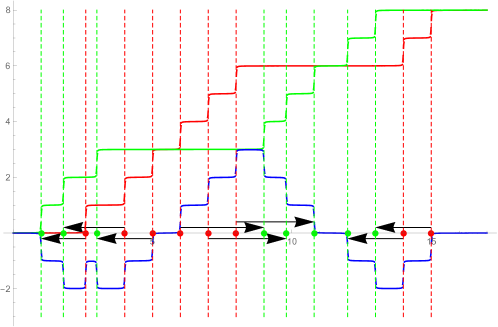
We define, for a given pair of spectra, the probability to observe a difference , if we pick a random value from their support (which approaches as increases, leaving out a negligible and decreasing number of levels),
| (10) |
The argument of the Kronecker delta function is an integer. The function equals unity if that integer is zero and vanishes otherwise. Note that Eq. (10) refers to a single matrix and that the integration measure is not modulated by the semicircle density. Clearly . Furthermore we have
| (11) | |||||
| (12) | |||||
| (13) |
For a permutation of diagonal matrix elements the trace of the matrix is conserved and hence, according to Eq. (13) the integral over of the spectral shift vanishes identically. While this is not the case for the other two perturbations that were considered above, it still holds after an ensemble average. Therefore we define desymmetrized moments
| (14) |
In the sequel we shall deal exclusively with the first two moments . As for they obey . Equality holds if the spectral shift takes only the values , . In particular Weyl’s rule implies that this is the case for . In analogy to Eq. (12), for the first moment a representation in terms of eigenvalue shifts can be found
| (15) | |||||
| (16) |
This can be understood from Fig. 1. All arrows from to crossing a given point have the same direction because the spectra are ordered. Thus is just the number of arrows crossing implying that the contribution of each arrow to the integral in (15) corresponds to its length . Similarly, based on Fig. 1, it is possible to derive an expression for the second moment, which is more involved and clarifies in more detail the relation between and .
1.2.2 The distribution of single eigenvalue shifts.
We consider the shift of individual eigenvalues
| (17) |
scaled by the global mean level spacing
| (18) |
in order to remove the dependence on the matrix size . For a pair of spectra we define the probability distribution
| (19) |
In terms of Fig. 1 can be interpreted as the distribution of directed arrow lengths. As in the distribution of the spectral shift function we use in Eq. (19) the whole spectrum of a single realization without taking into account the dependence of the mean level spacing on and, in the present section, do not consider ensemble averages.
The desymmetrized moments of the distribution are denoted by
| (20) | |||||
| (21) |
Again we shall study explicitly only the lowest two moments . Comparing Eqs. (16), (21) and using Eq. (18) we have for
| (22) |
A rough estimate for can be obtained on the basis of the Hoffman-Wielandt
inequality [3]:
Let and be two Hermitian matrices of dimension and the
spectra and be arranged in an increasing order.
Then, for any real with
| (23) |
where the p-norm of a vector is .
In our case and . Clearly, the application of this inequality is simplest when studying the processes (i) and (ii) where the perturbation is a diagonal matrix with non-zero entries. Below, in Section 2.2, we shall apply the Hoffman-Wielandt estimate in the discussion of the random replacement process.
2 The spectral variation for modified diagonal elements
We continue by addressing the effect of the replacement of diagonal elements by newly generated random entries, or the permutation of diagonal entries, on the spectrum of a Gaussian random matrix. In the first three subsections we derive analytical expressions for the spectral measures. The comparison with numerical simulations and the discussion of the results will be deferred to Section 2.4.
2.1 First-order perturbation theory
We generally consider ensemble averages of the spectral measures introduced in the previous section, , , but omit the explicit notation for ensemble averages over these quantities. We start with and show that in a certain range of it has a Gaussian distribution with known variance . This allows the computation of the two lowest moments of the spectral shift function. The crucial observation is, that for the Gaussian matrix ensembles, first order perturbation theory for the spectral differences can be justified in the limit of large and . Explicitly, first-order perturbation theory entails the result that the change of eigenvectors induced by the perturbation is of second order only, and accordingly yields for the permutation process
| (24) |
and for the random replacement process
| (25) |
where and are the eigenvector and the eigenvalue of the unperturbed matrix . To estimate the magnitude of these terms, recall the scaling of the matrix elements introduced in Section 1.1, namely . Thus, the terms in parantheses are of order . Furthermore, because of the uniform distribution of the eigenvectors and their normalization, the expansion coefficients are of order . Therefore the summands in (24), (25) are identically distributed random variables with zero mean and a finite variance . We will argue below that they can be considered as statistically independent. Hence the variance grows linearly in and the sums are of order , where is defined as . Comparing this to the mean level spacing we conclude that , i.e. for () the eigenvalue shifts are much smaller than the mean level spacing and perturbation theory is applicable. On the other hand, for () the eigenvalue shifts are of the order of the mean spacing. Then effects beyond first order perturbation theory such as avoided level crossings will become important.
In order to substantiate the above estimates we need to determine the statistics of the summands in (24), (25). First we note that the unit-norm eigenvectors of Gaussian random matrices can be converted under the transformation associated with their universality class into any arbitrary unit-norm vector. Consequently, the only requirement on the expansion coefficients is that their normalization remains unchanged. Accordingly, for large the are statistically independent and follow the Porter-Thomas distribution [10, 18, 19]
| (26) |
Thus, and for the three values of . The method used in Ref. [10] to derive Eq. (26) can be readily generalized to prove that the joint probablity distribution of expansion coefficients of a given eigenvector can be approximately factorized with an error of order . Second, the variances of the diagonal elements are , see Section 1.1. Now each term in the sums (24), (25) is of the form (where not necessarily equals ) or . The computation is simple for the latter expression since and the eigenvectors of are statistically independent from each other. We find
| (27) |
where the constant
| (28) |
takes the values 3 for GOE, 1 for GUE and 3/8 for GSE, respectively.
The computation of the mean and variance of is more involved since the eigenvectors of are statistically correlated with the matrix elements. However, we can use the spectral decomposition of yielding
| (29) |
The spectral parameters which appear in this expression are statistically independent for the Gaussian ensembles. In particular, and . Using the fact that , and we get for ,
| (30) |
This expression coincides with (27) as expected from the statistical independence of the different components of the eigenvectors. A slightly more involved computation for the case gives,
| (31) |
where the derivation of the higher-order term is quite lengthy but straight forward. Comparing (30) and (31) with (27), we conclude that in the limit of large , one can consider the eigenvectors and the diagonal matrix elements as statistically independent variables. In the following we apply these intermediate results to the two perturbation processes which are of interest in this paper.
2.2 Random replacements of diagonal matrix elements
For , the right hand side of Eq. (25) can be approximated as a sum of independent and identically distributed terms with the known variance . Hence, the variance of , averaged over and the ensemble, is
| (32) |
and thus
| (33) |
Furthermore, for large , the arguments presented in the previous section allow to apply the Central Limit Theorem to the right hand side of Eq. (25). Hence, the quantities distribute normally with zero mean and with variance , that is, to leading order in the ensemble average of the distribution (19) of scaled level shifts is Gaussian and independent of ,
| (34) |
yielding the mean value of
| (35) |
Note that for the typical eigenvalue shift is much smaller than the mean level spacing and it is expected that the spectral shift function is almost always bounded in absolute value by . Hence we have in this case
| (36) |
We will discuss the accuracy of this result in Sec. 2.4 and its implications in the Conclusions Sec. 4.
It is interesting to compare our results with the bounds provided by the Hoffman-Wielandt inequality (23). The l.h.s. contains a sum over a power of the eigenvalue shifts, while on the r.h.s. the diagonal elements of the perturbation are summed up. We find
| (37) |
The perturbation matrix has Gaussian distributed diagonal entries with variance and mean absolute value . Thus
| (38) | |||||
| (39) |
The variance as given by (33) is compatible with (39) for . On the other hand, after substitution of (35), equality holds in (38) for which is for , for and for . For smaller the inequality contradicts our result (35) for which is valid for .
2.3 Permuting diagonal matrix elements
There are two features which render the treatment of the permutation process more involved than the study of the randomization discussed above. The first one is that under permutations, both and do not vary with . This invariance might impose constraints on the spectral shift which do not exist in the treatment of the randomization process and could restrict the applicability of first-order perturbation which was the prerequisite for the derivations in the previous case. To check this possibility, recall the first order expression for the eigenvalue difference (24):
| (40) |
Then,
| (41) | |||||
since the last sum over gives . Thus, first order perturbation theory preserves . However perturbation theory fails to comply with the demand . To leading order
| (42) | |||||
This term is of order , and it can be neglected in comparison to the expected value of . Therefore, first-order perturbation theory is not ruled out by the invariance of the trace of under a permutation of diagonal elements.
The second feature which complicates the study of the permutation process is that the terms in the sum (40) are correlated, and the correlations depend on the decomposition of into irreducible cycles. To illustrate the difficulties which arise due to these correlations, we shall consider two examples. In the first, which applies to even only, is chosen as a product of cycles of length 2. It can be always presented as where . Then with Eq. (24),
| (43) |
The terms in the sum are uniformly distributed with zero mean and they are statistically independent since each term refers to a unique -cycle. The Porter-Thomas distribution gives . Thus, with the definition
| (44) |
the variance of each term in (43) is . A factor 2 has been introduced here because the sum (43) contains only terms. After this modification we can follow the same steps as previously for randomized diagonal elements and recover Eqs. (33), (34) and (35) with replaced by .
The second example to be considered is a cyclic permutation . Writing and , we can write with Eq. (24) the spectral difference as
| (45) | |||||
| (46) |
Clearly, every term in the sum is correlated with its predecessor. Therefore the Central Limit Theorem cannot be used as was previously done in the derivation of Eqs. (34) and (35) and will be replaced by the Martingale Central Limit Theorem. Calling the sum in (46) and removing the first term we get
| (47) |
which has the following properties making it a martingale:
-
-
.
-
-
The expectation value of conditioned on having specific values equals .
The second property follows from the fact that
| (48) |
where distributes independently of in the large limit with .
Moreover, since the distribution of both the diagonal matrix elements of and the squared amplitudes of the eigenvectors decay exponentially fast, the Lindeberg condition [20] is satisfied. Therefore the distribute normally with variance where is the variance of any single summation term in Eq. (47). For large this result cannot be substantially changed by the missing term such that also distributes normally with variance . We are grateful to Jonathan Breuer for providing us with a formal proof of this claim [21].
The result above shows that the mean spectral measures for the two extreme permutations involving the smallest and the largest cycle length, respectively, are identical. However, general permutations can display a more complicated cycle structure than the ones discussed above. A general permutation can be written as a product of cycles of lengths , and . The sum (24) can be divided into the contribution of statistically independent sums over cycles of period . The number of permutations of numbers, with cycles is given by the Stirling number of the first kind [22]. Considering a random permutation, it is known [23] that for large t, the distribution of the number of cycles is approximately normal with mean and variance , where is the Euler constant. Hence, most cycles are long, with of order . Therefore, by using the previous result, their contribution will be normally distributed with variance and their sum will be distributed normally with variance .
We end this section by summarizing the results obtained for the spectral measures in the case of permutations of diagonal matrix elements:
| (49) |
| (50) |
2.4 Simulations and error estimates
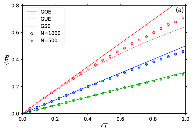
(a) Comparison of numerical results for the variance of individual eigenvalue shifts (dots) with results from Eq. (33) (straight lines) for GOE (red), GUE (blue), and GSE (green). Note that the axes are vs. . This scaling makes the horizontal axis compatible to that in Fig. 3b and maps our prediction on a straight line in order to highlight the nature of deviations. The dashed line is a phenomenological correction of perturbation theory taking into account the re-ordering of the spectra when levels cross (see text).
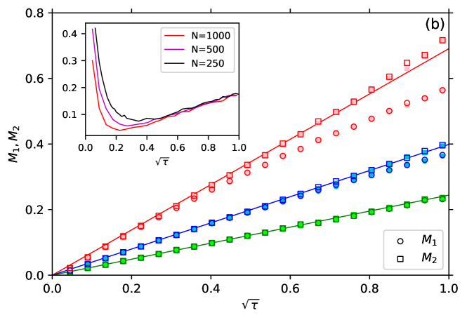
(b) Numerical results for the first two moments of the spectral shift. The color code is the same as in Fig. 3a. The straight line is the perturbative result for the first moment given in Eq. (36). The inset shows the relative deviation of from this prediction for the GOE. Additional colors are used here to display results for and .

In this section we compare our theoretical predictions to numerical simulations in order to verify and illustrate the results as well as to discuss their range of applicability. All numerical ensemble averages are based on 5000 realizations. For GSE () the standard representation of quaternions by matrices was used which requires the diagonalization of a matrix. It yields a doubly degenerate spectrum from which half of the eigenvalues were discarded.
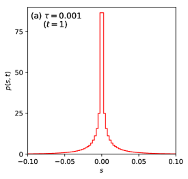
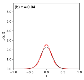
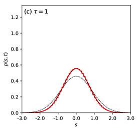
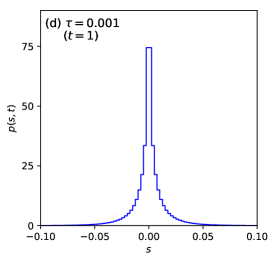
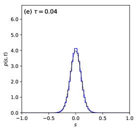
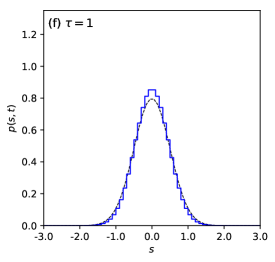
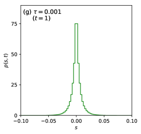
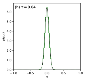
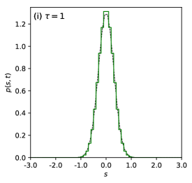
We first address in some detail the random replacement process. Fig. 2 shows the ensemble averaged distribution of rescaled eigenvalue shifts for all three values of . The selected numbers of randomized matrix elements correspond to three regimes of to be discussed below. Qualitatively we observe a distribution which is sharply peaked at zero when only few terms contribute in Eq. (25). It evolves into a Gaussian distribution as grows. Note the varying scale on the horizontal axis. For small (left column) typical eigenvalue shifts are much smaller than the mean level spacing () while for maximal perturbation (right column) they are of the order of (). The dashed lines in the middle and right columns show our analytical result from Eq. (34). Agreement is best for GSE while for GOE there remain substantial deviations from our theory. Therefore we will concentrate on the GOE in the following and try to establish the range of applicability of our predictions.
Fig. 3a shows the dependence on of the variance of the distributions from Fig. 2. Note the scaling vs. which was chosen for compatibility with Fig. 3b. The data for GOE are displayed with pink and red color for two different matrix sizes and , respectively. Up to uncertainties due to the finite sample size, the results are independent of . Our analytical result (33) is plotted as straight red line. As we can see this prediction is valid for small values of but overestimates the eigenvalue shifts for . Besides the gradual failure of perturbation theory for increasing this behavior can also be attributed to level crossings which are not captured by our perturbative treatment since the spectral measures we adopted are sensitive to the ordering of eigenvalues. Indeed, even if the perturbative results and correctly describe the shifts of two neighboring eigenvalues there can be situations where , i.e. the levels cross. This would imply that the perturbed spectrum is reordered such that and . In this case the values for the eigenvalue shifts entering the calculation of are smaller than the actual perturbative shifts. Such a failure of the perturbative approach is more likely for large perturbative eigenvalue shifts, i.e. for growing . It is also more likely if the probability of a small level spacing is large. Therefore the deviation of our theory from the data is considerably smaller for the GUE (Fig. 2d-f and blue symbols in Fig. 3a) where the level repulsion is stronger and it is even smaller for GSE (green symbols). To illustrate the effect of level crossings we have calculated for GOE the perturbative spectrum numerically, reordered it in an increasing sequence and then determined the distribution of eigenvalue shifts. The result for the associated second moment is plotted in Fig. 3a as dashed line. It is closer to the actual data but now underestimates the eigenvalue shifts. Thus, in order to get a substantially better theoretical result it will be necessary to go beyond first-order perturbation theory and to properly take into account the interaction between the eigenvalues which becomes manifest, e.g. in avoided level crossings. Yet, the essence of the behavior of for the various universality classes is already contained in our analytical results.
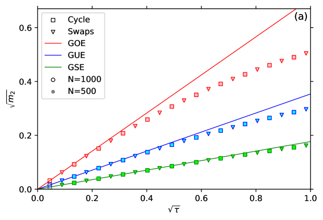
(a) Comparison of numerical results for the variance of individual eigenvalue shifts to the perturbative result (straight lines), see Eqs. (49), (44). Note that the axes scaling are vs. .
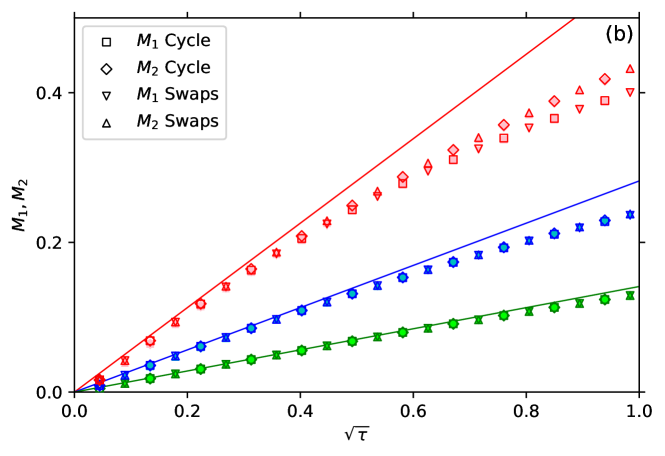
(b) Numerical results for the first two moments of the spectral shift. The color code is the same as in (a). The straight lines show the perturbative result for the first moment, see Eqs. (44), (50).
In Fig. 3b the first two moments of the spectral shift are shown. According to Eq. (35), and thus on first glance the data for (red circles) show a behavior that is very similar to Fig. 3a. However, for small there are now deviations which were absent in Fig. 3a. They are magnified in the inset of Fig. 3b where the relative difference between the simulations and our result is plotted. Indeed the proportionality between and the first moments relies on the validity of the Central Limit Theorem which fails for small . Consider the extreme case (). Taking the absolute value and summing over in Eq. (25) yields . The r.h.s has mean value such that is the correct perturbative result for the first moment. Its deviation from Eq. (35), , is about which is the maximal value in the inset of Fig. 3b. For increasing the deviation decreases to a minimum before it grows again. For this minimum corresponds to the distribution shown in Fig. 2b (). It is a compromise between the error in the Central Limit Theorem for small and the error in perturbation theory for large . The minimal deviation decreases as increases and at the same time it is reached for smaller values of such that Eq. (35) is valid with increasing precision and in a growing range.
As explained below Eq. (14), the first two moments of the spectral shift are related by with equality holding when the distribution is limited to values . This is confirmed by Figs. 3b and 4. For small the average eigenvalue shift is much smaller than the mean level spacing (Fig. 2a,b) and therefore the spectral shift typically does not exceed one (Fig. 4a,b). In Fig. 3b we observe that the data for coincide in this regime. Beyond that range the data for grow faster and happen to be quite close to the perturbative prediction for but we have no quantitative explanation for this observation.
Fig. 5 shows and for the two types of permutations of diagonal matrix elements which were discussed in detail in Section 2.3. Squares represent a single cycle of length while triangles represent cycles of length 2. As expected, both types of permutations lead to similar results which for small approach our predictions. The qualitative behavior is very similar to randomized diagonal elements (Fig. 3) but the relative deviation from our theory is slightly larger. In Fig. 5b there is again a minimal deviation for at some intermediate value of compromising between perturbation theory and Central Limit Theorem which are valid for small and large , respectively. In contrast to Fig. 3, the difference between and is smaller now such that for the second moment of the spectral shift remains well below our perturbative result for .
The behavior of GOE, GUE and GSE is qualitatively very similar in both, Fig. 3 and Fig. 5. The only difference is in the magnitude of the deviations from our theory which is decreasing with increasing . We attribute this to the increasing level repulsion from GOE to GSE which implies a lower probability of small level spacings. Thus, also perturbative level crossings (or avoided crossings of levels under the perturbation), which were identified above as an important source of deviations, have less influence.
3 Random replacement of columns and rows
The process (iii) defined in the Introduction differs considerably from the two processes (i) and (ii) discussed previously: once it is completed at the resulting matrix is completely independent of the reference matrix, in stark contrast to processes (i) and (ii) where only the diagonal matrix elements are affected by the perturbation.
We shall start this section by explaining why the perturbative approach of Section 2 fails for process (iii). Using Eq. (4) first-order perturbation theory yields
where is a randomly chosen matrix from the respective ensemble. The sums differ in the number of their summands, and in their variances. Each of them is composed of independent and identically distributed random numbers. Thus, in the limit of large and we can apply for each sum the Central Limit Theorem. The first sum coincides with Eq. (25) and yields a level shift of the order of the mean level spacing or below, as shown in Section 2.2. Furthermore, the scaling with is of the same order of magnitude for each summand of both sums. However, the number of terms in the second sum is larger by a factor . Thus, this sum compared to the mean level spacing is larger by a factor growing to infinity . Accordingly, first-order perturbation theory fails.
So far we cannot offer a complete theory for the process (iii). However, we will present numerical and analytical approaches towards an understanding of the scaling of the spectral shift with the parameters , and .
The fact that the matrices and the reference matrix are statistically independent can be used to establish constraints on the variance . In Eq. (1) the average spectral counting function is introduced which is independent of . We consider the fluctuations of the actual spectral counting function around , . Then
| (52) | |||||
The two integrals bracketed in the square parentheses correspond to leading order in to the number variance introduced by Dyson [24] which, in the limit of large , is well approximated by [4]
| (53) |
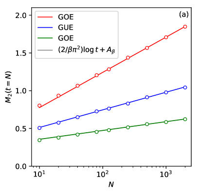
where is independent of . The third integral is zero due to the absence of correlations between and . Thus we expect that the variance for grows logarithmically with ,
| (54) |
Indeed this is confirmed in Fig. 6a. The constant is known explicitly in random matrix theory. There the eigenvalues, the spectral density of which is given by the semicircle law, are unfolded to uniform density. We, however, use raw spectra for the computation of . Accordingly, we have determined by fitting Eq. (54) to the numerical curves.
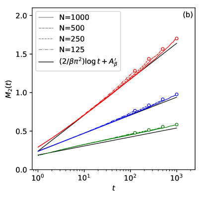
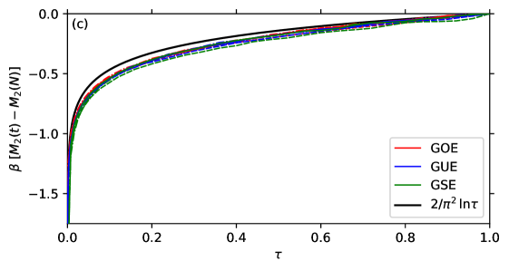
In Fig. 6b the dependence of on is shown for 125, 250, 500 and 1000. A remarkable numerical observation is that these curves all fall on top of each other when is not too close to its maximum value . For each ensemble a logarithmic increase is observed with a slope and a constant close to the values from (54), i.e. we have
| (55) |
The numerical data follow this law for a range of which is growing with . Note however, that the case with is not shown in Fig. 6b because of the logarithmic scale.
Finally, in Fig. 6c we show the data from Fig. 6b in a different representaion where the endpoints of all curves coincide. Namely we consider the quantity . According to Eq. (55) it can be represented as a function of and is inversely proportional to ,
| (56) |
Indeed, when scaled by , the curves for all matrix sizes and all ensembles essentially fall on top of each other as shown in Fig. 6c. An exception is the case where a logarithmic singularity develops.
Thus, we may conclude that a perturbation randomizing rows and the corresponding columns of the reference matrix leads to plus some lower-order corrections including a constant term . Further work is needed to obtain a more accurate description of these corrections. It could be based, e.g., on the supersymmetric approach to random-matrix theory [25, 26, 27, 28].
4 Conclusions
We have studied the effect of perturbations of rank on the spectra of Gaussian random matrices. Among other spectral measures we considered the variance of the spectral shift function. From the virtually unlimited number of possibilities to define perturbations of a given rank we chose two quite disparate cases, one where only diagonal elements are affected and one where entire rows and columns are randomized. In the first case we obtain a satisfactory theory using first-order perturbation theory. In the second case perturbation theory fails and we have no complete analytical theory at the moment. However, we established numerically the scaling of the spectral shift with the parameters and . While in the first case all spectral measures considered can be expressed in terms of scaled variable alone, in the second case there is an additional dependence on the matrix size .
It is definitely possible to extend our results beyond the considered perturbation models. For example, if we randomize a quadratic block of size we have a case which interpolates between the two cases we studied and we observe a crossover between perturbation theory for small and the case of two completely uncorrelated matrices at .
One central result for the case of a diagonal perturbation is that the variance of the spectral shift increases as (Eqs. (36) and (50)) with some constant . This holds for in a parameter range where is large but is small. The numerically observed range of validity is increasing with so that it covers the entire range of for the GSE, is slightly confined for GUE and is limited to small for GOE.
An interesting interpretation of this result arises if we consider as time and the gradually growing spectral variation as a dynamic process. At each time step there is a slight variation of the spectrum, e.g. by randomizing another diagonal element. These steps result in a random walk in the spectral shift distribution where the resulting mean probability distribution displays anomalous diffusion (subdiffusion) in the "time" . The "diffusion coefficient" depends on the type of perturbation and the random matrix ensemble under study. This behavior can be compared to the spectral shift statistics of a different model, namely the Anderson model in one dimension which corresponds to an ensemble of Jacobi matrices with random iid diagonal elements and on the secondary diagonals. Heuristic arguments supported by some estimates suggest that in this case the variance of the spectral shift due to interchanging or randomizing diagonal elements grows linearly with . Numerical simulations confirm this intuition [29]. In other words, the Poissonian nature of the spectrum seems to lead to standard diffusion of the spectral shift.
Anomalous diffusion with variance which grows in time as occurs in several systems which were studied in statistical mechanics out of equilibrium. Particularly similar to the system under study in the present article is the single file tracer model, in which particles are confined to a tube and scatter elastically when they get closer, but are unable to penetrate each other. The displacements of tracer particles are known to be sub-diffusive with the variance proportional to the square root of the time. It was recently shown [30] that a transition to regular diffusion, with a variance growing linearly in time, occurs once particles are allowed to interchange their position. The question whether this similarity to our problem is rooted in the dynamics of the two systems, or it is just incidental, remains to be addressed.
Acknowledgements
Michael Aizenman and Jonathan Breuer introduced US to the martingale concept and its application in the present case. Thanks to both. In particular we are obliged to Jonathan who provided us with a lemma on and its proof, used in the discussion of equations (41-44). We thank David Mukamel for pointing out the possible connection between the single file tracer model and the present work. B.D. thanks the NNSF of China for financial support under grant Nos. 11775100 and 11961131009 and the Weizmann Institute of Science for financial support and hospitality.
References
References
- [1] Weyl H 1912 Mathematische Annalen LXXI 441–479
- [2] Birman M Sh and Yafaev D R 1993 St. Petersburg Math. J. 4 833–870
- [3] Hoffman A J and Wielandt H W 1953 Duke Math. J. 20 37–39
- [4] Mehta M L 1990 Random matrices 2nd ed (Pure and Applied Mathematics vol 142) (Academic Press)
- [5] Smolyarenko I E and Simons B D 2003 Journal of Physics A: Mathematical and Theoretical 36 3551–3567
- [6] Aleiner I L and Matveev K A 1998 Phzsical Review Letters 80 814–816
- [7] Bohigas O, Giannoni M J and Schmit C 1986 Spectral fluctuations of classically chaotic quantum system Quantum Chaos and Statistical Nuclear Physics ed Seligman T H and Nishioka H (Berlin: Springer)
- [8] Giannoni M J, Voros A and Zinn-Justin J (eds) 1991 Chaos and quantum physics Session LII of the Les Houches Summer School of Theoretical Physics, 1989 (Amsterdam: North-Holland)
- [9] Guhr T, Müller-Groeling A and Weidenmüller H A 1998 Phys. Rep. 299 190–425
- [10] Haake F 2010 Quantum Signatures of Chaos 3rd ed (Springer)
- [11] Berkolaiko G, Kennedy J, Kurasov P and Mugnolo D 2019 Transactions of the American Mathematical Society 372 5153–5197
- [12] Aizenman M, Schanz H, Smilansky U and Warzel S 2017 Acta Physica Polonica A 132 1699–1703
- [13] Schanz H and Smilansky U 2019 St. Petersburg Mathematical Journal 30 591–600
- [14] Yunko V, Białous M and Sirko L 2020 Phys. Rev. E 102(1) 012210
- [15] Kottos T and Smilansky U 1999 Ann. Phys. 274 76–124
- [16] Pluhař Z and Weidenmüller H A 2015 Journal of Physics A: Mathematical and Theoretical 48 275102
- [17] Gnutzmann S and Altland A 2004 Phys. Rev. Lett. 93(19) 194101
- [18] Alonso L and Gorin T 2016 J. Phys. A 49 145004
- [19] Pandey A, Kumar A and Puri S 2019 arXiv e-prints arXiv:1905.10596
- [20] M B Brown B M 1971 Ann. Math. Stat. 42 59–66
- [21] Breuer J, private communication
- [22] Vialar T 2016 Handbook of Mathematics (Norderstedt: Books on Demand)
- [23] Louchard G 2010 Discrete Mathematics and Theoretical Computer Science 12 167–184 Discrete Mathematics and Theoretical Computer Science. 12, 167-184 (2010).
- [24] Dyson F J and Mehta M L 1963 Journal of Mathematical Physics 4 701–712
- [25] Verbaarschot J J M, Weidenmüller H A and Zirnbauer M R 1985 Phys. Rep. 129 367–438
- [26] Guhr T and Weidenmüller H A 1990 Annals of Physics 199 412–446
- [27] Guhr T 1991 Journal of Mathematical Physics 32 336–347
- [28] Joyner C H, Smilansky U and Weidenmüller H A 2017 Journal of Physics A Mathematical General 50 385101
- [29] Dietz B, Schanz H and Smilansky U, in preparation.
- [30] Miron A, Mukamel D and Posch H A 2020 Journal of Statistical Mechani cs: Theory and Experiment 2020 063216