Meta-Sim2: Unsupervised Learning of Scene Structure for Synthetic Data Generation
Abstract
Procedural models are being widely used to synthesize scenes for graphics, gaming, and to create (labeled) synthetic datasets for ML. In order to produce realistic and diverse scenes, a number of parameters governing the procedural models have to be carefully tuned by experts. These parameters control both the structure of scenes being generated (e.g. how many cars in the scene), as well as parameters which place objects in valid configurations. Meta-Sim aimed at automatically tuning parameters given a target collection of real images in an unsupervised way. In Meta-Sim2, we aim to learn the scene structure in addition to parameters, which is a challenging problem due to its discrete nature. Meta-Sim2 proceeds by learning to sequentially sample rule expansions from a given probabilistic scene grammar. Due to the discrete nature of the problem, we use Reinforcement Learning to train our model, and design a feature space divergence between our synthesized and target images that is key to successful training. Experiments on a real driving dataset show that, without any supervision, we can successfully learn to generate data that captures discrete structural statistics of objects, such as their frequency, in real images. We also show that this leads to downstream improvement in the performance of an object detector trained on our generated dataset as opposed to other baseline simulation methods. Project page: https://nv-tlabs.github.io/meta-sim-structure/.
1 Introduction
Synthetic datasets are creating an appealing opportunity for training machine learning models e.g. for perception and planning in driving [55, 18, 53], indoor scene perception [46, 57], and robotic control [61]. Via graphics engines, synthetic datasets come with perfect ground-truth for tasks in which labels are expensive or even impossible to obtain, such as segmentation, depth or material information. Adding a new type of label to synthetic datasets is as simple as calling a renderer, rather than embarking on a time consuming annotation endeavor that requires new tooling and hiring, training and overseeing annotators.
Creating synthetic datasets comes with its own hurdles. While content, such as 3D CAD models that make up a scene are available on online asset stores, artists write complex procedural models that synthesize scenes by placing these assets in realistic layouts. This often requires browsing through massive amounts of real imagery to carefully tune a procedural model – a time consuming task. For scenarios such as street scenes, creating synthetic scenes relevant for one city may require tuning a procedural model made for another city from scratch. In this paper, we propose an automatic method to carry out this task.
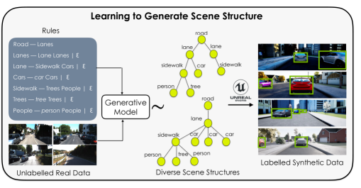
Recently, Meta-Sim [30] proposed to optimize scene parameters in a synthetically generated scene by exploiting the visual similarity of (rendered) generated synthetic data with real data. They represent scene structure and parameters in a scene graph, and generate data by sampling a random scene structure (and parameters) from a given probabilistic grammar of scenes, and then modifying the scene parameters using a learnt model. Since they only learn scene parameters, a sim-to-real gap in the scene structure remains. For example, one would likely find more cars, people and buildings in Manhattan over a quaint village in Italy. Other work on generative models of structural data such as graphs and grammar strings [37, 12, 17, 42] require large amounts of ground truth data for training to generate realistic samples. However, scene structures are extremely cumbersome to annotate and thus not available in most real datasets.
In this paper, we propose a procedural generative model of synthetic scenes that is learned unsupervised from real imagery. We generate scene graphs object-by-object by learning to sample rule expansions from a given probabilistic scene grammar and generate scene parameters using [30]. Learning without supervision here is a challenging problem due to the discrete nature of the scene structures we aim to generate and the presence of a non-differentiable renderer in the generative process. To this end, we propose a feature space divergence to compare (rendered) generated scenes with real scenes, which can be computed per scene and is key to allowing credit assignment for training with reinforcement learning.
We evaluate our method on two synthetic datasets and a real driving dataset and find that our approach significantly reduces the distribution gap between scene structures in our generated and target data, improving over human priors on scene structure by learning to closely align with target structure distributions. On the real driving dataset, starting from minimal human priors, we show that we can almost exactly recover the structural distribution in the real target scenes (measured using GT annotations available for cars) – an exciting result given that the model is trained without any labels. We show that an object detector trained on our generated data outperforms those trained on data generated with human priors or by [30], and show improvements in distribution similarity measures of our generated rendered images with real data.
2 Related Work
2.1 Synthetic Content Creation
Synthetic content creation has been receiving significant interest as a promising alternative to dataset collection and annotation. Various works have proposed generating synthetic data for tasks such as perception and planning in driving [55, 18, 53, 14, 48, 68, 2], indoor scene perception [70, 75, 46, 57, 59, 24, 4], game playing [6, 28], robotic control [61] [6, 63, 56], optical flow estimation [7, 58], home robotics [49, 34, 20] amongst many others, utilizing procedural modeling, existing simulators or human generated scenarios.
Learnt Scene Generation brings a data-driven nature to scene generation. [74, 64] propose learning hierarchical spatial priors between furniture, that is integrated into a hand-crafted cost used to generate optimized indoor scene layouts. [50] similarly learn to synthesize indoor scenes using a probabilistic scene grammar and human-centric learning by leveraging affordances. [64] learn to generate intermediate object relationship graphs and instantiate scenes conditioned on them. [76] use a scene graph representation and learn adding objects into existing scenes. [54, 40, 65] propose methods for learning deep priors from data for indoor scene synthesis. [16] introduce a generative model that sequentially adds objects into scenes, while [29] propose a generative model for object layouts in 2D given a label set. [60] generate batches of data using a neural network that is used to train a task model, and learn by differentiating through the learning process of the task model. [30] propose learning to generate scenes by modifying the parameters of objects in scenes that are sampled from a probabilistic scene grammar. We argue that this ignores learning structural aspects of the scene, which we focus on in our work. Similar to [30, 16], and contrary to other works, we learn this in an unsupervised manner i.e. given only target images as input.
Learning with Simulators: Methods in Approximate Bayesian Inference have looked into inferring the parameters of a simulator that generate a particular data point [45, 35]. [11] provide a great overview of advances in simulator based inference. Instead of running inference per scene [35, 69], we aim to generate new data that resembles a target distribution. [44] learn to optimize non-differentiable simulators using a variational upper bound of a GAN-like objective. [8] learn to optimize simulator parameters for robotic control tasks by directly comparing trajectories between a real and a simulated robot. [19, 47] train an agent to paint images using brush strokes in an adversarial setting with Reinforcement Learning. We learn to generate discrete scene structures constrained to a grammar, while optimizing a distribution matching objective (with Reinforcement Learning) instead of training adversarially. Compared to [47], we generate large and complex scenes, as opposed to images of single objects or faces.
2.2 Graph Generation
Generative models of graphs and trees [42, 17, 73, 43, 10, 3] generally produce graphs with richer structure with more flexibility over grammar based models, but often fail to produce syntactically correct graphs for cases with a defined syntax such as programs and scene graphs. Grammar based methods have been used for a variety of tasks such as program translation [9], conditional program generation [71, 72], grammar induction [32] and generative modelling on structures with syntax [37, 12], such as molecules. These methods, however, assume access to ground-truth graph structures for learning. We take inspiration from these methods, but show how to learn our model unsupervised i.e. without any ground truth scene graph annotations.
3 Methodology
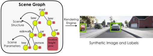
We aim to learn a generative model of synthetic scenes. In particular, given a dataset of real imagery , the problem is to create synthetic data of images and labels that is representative of , where represents the parameters of the generative model. We exploit advances in graphics engines and rendering, by stipulating that the synthetic data is the output of creating an abstract scene representation and rendering it with a graphics engine. Rendering ensures that low level pixel information in (and its corresponding annotation ) does not need to be modelled, which has been the focus of recent research in generative modeling of images [31, 51]. Ensuring the semantic validity of sampled scenes requires imposing constraints on their structure. Scene grammars use a set of rules to greatly reduce the space of scenes that can be sampled, making learning a more structured and tractable problem. For example, it could explicitly enforce that a car can only be on a road which then need not be implicitly learned, thus leading us to use probabilistic scene grammars. Meta-Sim [30] sampled scene graph structures (see Fig. 2) from a prior imposed on a Probabilistic Context-Free Grammar (PCFG), which we call the structure prior. They sampled parameters for every node in the scene graph from a parameter prior and learned to predict new parameters for each node, keeping the structure intact. Their generated scenes therefore come from a structure prior (which is context-free) and the learnt parameter distribution, resulting in an untackled sim-to-real gap in the scene structures. In our work, we aim to alleviate this by learning a context-dependent structure distribution unsupervised of synthetic scenes from images.
We utilize scene graphs as our abstract scene representation, that are rendered into a corresponding image with labels (Sec 3.1). Our generative model sequentially samples expansion rules from a given probabilistic scene grammar (Sec 3.2) to generate a scene graph which is rendered. We train the model unsupervised and with reinforcement learning, using a feature-matching based distribution divergence specifically designed to be amenable to our setting (Sec 3.3).

3.1 Representing Synthetic Scenes
In Computer Graphics and Vision, Scene Graphs are commonly used to describe scenes in a concise hierarchical manner, where each node describes an object in the scene along with its parameters such as the 3D asset, pose etc. Parent-child relationships define the child’s parameters relative to its parent, enabling easy scene editing and manipulation. Additionally, camera, lighting, weather etc. are also encoded into the scene graph. Generating corresponding pixels and annotations amounts to placing objects into the scene in a graphics engine and rendering with the defined parameters (see Fig. 2).
Notation: A context-free grammar is defined as a list of symbols (terminal and non-terminal) and expansion rules. Non-terminal symbols have at least one expansion rule into a new set of symbols. Sampling from a grammar involves expanding a start symbol till only non-terminal symbols remain. We denote the total number of expansion rules in a grammar as . We define scene grammars and represent strings sampled from the grammar as scene graphs following [48, 30] (see Fig. 3). For each scene graph, a structure is sampled from the grammar followed by sampling corresponding parameters for every node in the graph.
3.2 Generative Model
We take inspiration from previous work on learning generative models of graphs that are constrained by a grammar [37] for our architecture. Specifically, we map a latent vector to unnormalized probabilities over all possible grammar rules in an autoregressive manner, using a recurrent neural network till a maximum of steps. Deviating from [37], we sample one rule at every time step and use it to predict the logits for the next rule . This allows our model to capture context-dependent relationships easily, as opposed to the context-free nature of scene graphs in [30]. Given a list of at most sampled rules, the corresponding scene graph is generated by treating each rule expansion as a node expansion in the graph (see Fig. 3).
Sampling Correct Rules: To ensure the validity of sampled rules in each time step , we follow [37] and maintain a last-in-first-out (LIFO) stack of unexpanded non-terminal nodes. Nodes are popped from the stack, expanded according to the sampled rule-expansion, and the resulting new non-terminal nodes are pushed to the stack. When a non-terminal is popped, we create a mask of size which is 1 for valid rules from that non-terminal and 0 otherwise. Given the logits for the next expansion , the probability of a rule is represented as,
Sampling from this masked multinomial distribution ensures that only valid rules are sampled as . Given the logits and sampled rules, , the probability of the corresponding scene structure given is simply,
Putting it together, images are generated by sampling a scene structure from the model, followed by sampling parameters for every node in the scene and rendering an image . For some , with parameters and structure , we assume111This equality does not hold in general for rendering, but it worked well in practice,
3.3 Training
Training such a generative model is commonly done using variational inference [33, 52] or by optimizing a measure of distribution similarity [22, 41, 39, 30]. Variational Inference allows using reconstruction based objectives by introducing an approximate learnt posterior. Our attempts at using variational inference to train this model failed due to the complexity coming from discrete sampling and having a renderer in the generative process. Moreover, the recognition network here would amount to doing inverse graphics – an extremely challenging problem [36] in itself. Hence, we optimize a measure of distribution similarity of the generated and target data. We do not explore using a trained critic due to the clear visual discrepancy between rendered and real images that a critic can exploit. Moreover, adversarial training is known to be notoriously difficult for discrete data. We note that recent work [19, 47] has succeeded in adversarial training of a generative model of discrete brush strokes with reinforcement learning (RL), by carefully limiting the critic’s capacity. We similarly employ RL to train our discrete generative model of scene graphs. While two sample tests, such as MMD [23] have been used in previous work to estimate and minimize the distance between two empirical distributions [41, 15, 39, 30], training with MMD and RL resulted in credit-assignment issues as it is a single score for the similarity of two full sets(batches) of data. Instead, our metric can be computed for every sample, which greatly helps training as shown empirically in Sec. 4.
Distribution Matching: We train the generative model to match the distribution of features of the real data in the latent space of some feature extractor . We define the real feature distribution s.t for some . Similarly we define the generated feature distribution s.t for some . We accomplish distribution matching by approximately computing from samples and minimizing the KL divergence from to . Our training objective is
Using the feature distribution definition above, we have the equivalent objective
| (1) |
The true underlying feature distributions and are usually intractable to compute. We use approximations and , computed using kernel density estimation (KDE). Let and be a batch of real and generated images. KDE with to estimate yield
where is the standard multivariate normal kernel with bandwidth matrix . We use where is the dimensionality of the feature space.
Our generative model involves making a discrete (non-differentiable) choice at each step, leading us to optimize our objective using reinforcement learning techniques222We did not explore sampling from a continuous relaxation of the discrete variable here. Specifically, using the REINFORCE [67] score function estimator along with a moving average baseline, we approximate the gradients of Eq. 1 as
| (2) |
where M is the batch size, and are density estimates defined above.
Notice that the gradient above requires computing the marginal probability of a generated image , instead of the conditional . Computing the marginal probability of a generated image requires an intractable marginalization over the latent variable . To circumvent this, we use a fixed finite number of latent vectors from a set sampled uniformly, enabling easy marginalization. This translates to,
We find that this still has enough modeling capacity, since there are only finitely many scene graphs of a maximum length that can be sampled from the grammar. Empirically, we find using one latent vector to be enough in our experiments. Essentially, stochasticity in the rule sampling makes up for lost stochasticity in the latent space.
Pretraining is an essential step for our method. In every experiment, we define a simple handcrafted prior on scene structure. For example, a simple prior could be to put one car on one road in a driving scene. We pre-train the model by sampling strings (scene graphs) from the grammar prior, and training the model to maximize the log-likelihood of these scene graphs. We provide specific details about the priors used in Sec 4.
Feature Extraction for distribution matching is a crucial step since the features need to capture structural scene information such as the number of objects and their contextual spatial relationships for effective training. We describe the feature extractor used and its training for each experiment in Sec 4.
Ensuring termination: During training, sampling can result in incomplete strings generated with at most steps. Thus, we repeately sample a scene graph until its length is at most . To ensure that we do not require too many attempts, we record the rejection rate of a sampled feature as the average failed sampling attempts when sampling the single scene graph used to generate . We set a threshold on (representing the maximum allowable rejections) and weight and add it to our original loss as,
We found that and worked well for all of our experiments.
4 Experiments
We show two controlled experiments, on the MNIST dataset [38] (Sec. 4.1) and on synthetic aerial imagery [30] (Sec. 4.2), where we showcase the ability of our model to learn synthetic structure distributions unsupervised. Finally, we show an experiment on generating 3D driving scenes (Sec. 4.3), mimicking structure distributions on the KITTI [21] driving dataset and showing the performance of an object detector trained on our generated data. The renderers used in each experiment are adapted from [30]. For each experiment, we first dicuss the corresponding scene grammar. Then, we discuss the feature extractor and its training. Finally, we describe the structure prior used to pre-train the model, the target data, and show results on learning to mimic structures in the target data without any access to ground-truth structures. Additionally, we show comparisons with learning with MMD [23] (Sec. 4.1) and show how our model can learn to generate context-dependent scene graphs from the grammar (Sec. 4.2).
4.1 Multi MNIST
We first evaluate our approach on a toy example of learning to generate scenes with multiple digits. The grammar defining the scene structure is:
Sampled digits are placed onto a black canvas of size .
Feature Extraction Network: We train a network to determine the binary presence of a digit class in the scene. We use a Resnet [26] made up of three residual blocks each containing two convolutional layers to produce an image embedding and three fully connected layers from the image embedding to make the prediction. We use the Resnet embeddings as our image features. We train the network on synthetic data generated by our simple prior for both structure and continuous parameters. Training is done with a simple binary cross-entropy criterion for each class. The exact prior and target data used is explained below.
Prior and Target Data: We sample the number of digits in the scene uniformly from to , and sample digits uniformly to place on the scene. The digits are placed(parameters) uniformly on the canvas. The target data has digits upright in a straight line in the middle of the canvas. Fig. 7 shows example prior samples, and target data. We show we can learn scene structures with a gap remaining in the parameters by using the parameter prior during training.

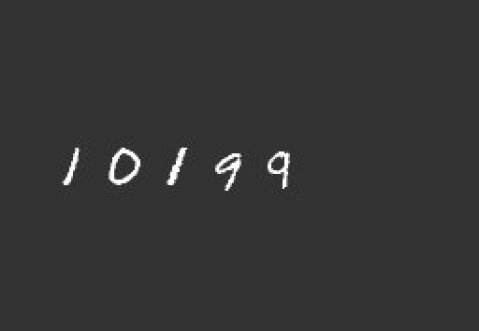
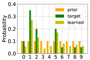
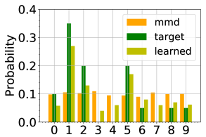
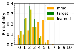
We attempt learning a random distribution of number of digits with random classes in the scene. Fig. 7 shows the prior, target and learnt distribution of the number of digits and their class distribution. We see that our model can faithfully approximate the target, even while learning it unsupervised. We also train with MMD [23], computed using two batches of real and generated images and used as the reward for every generated scene. Fig. 7 shows that using MMD results in the model learning a smoothed approximation of the target distribution, which comes from the lack of credit assignment in the score, that we get with our objective.
4.2 Aerial 2D
Next, we evaluate our approach on a harder synthetic scenario of aerial views of driving scenes. The grammar and the corresponding rendered scenes offer additional complexity to test the model. The grammar here is as follows:
Feature Extraction Network: We use the same Resnet [26] architecture from the MNIST experiment with the FC layers outputting the number of cars, roads, houses and trees in the scene as 1-hot labels. We train by minimizing the cross entropies these labels, trained on samples generated from the prior.
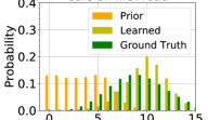
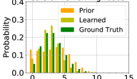
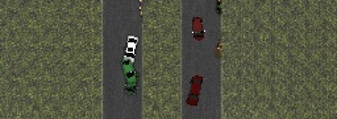
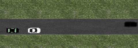
Prior: We sample the number of roads uniformly. On each road, we sample cars uniformly. Roads are placed sequentially by sampling a random distance and placing the road pixels in front of the previous one. Cars are placed on the road with uniform random position and rotation (Fig. 7).
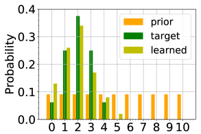
Learning context-dependent relationships: For the target dataset, we sample the number of roads with probabilities (0.05, 0.15, 0.4, 0.4). On the first road we sample cars and cars for each of the remaining roads. All cars are placed well spaced on their respective road. Unlike the Multi-MNIST experiment, these structures cannot be modelled by a Probabilistic-CFG, and thus by [37, 30]. We see that our model can learn this context-dependent distribution faithfully as well in Fig. 8.
4.3 3D Driving Scenes
We experiment on the KITTI [21] dataset, which was captured with a camera mounted on top of a car driving around the city of Karlsruhe, Germany. The dataset contains a wide variety of road scenes, ranging from urban traffic scenarios to highways and more rural neighborhoods. We utilize the same grammar and renderer used for road scenes in [30]. Our model, although trained unsupervised, can learn to get closer to the underlying structure distribution, improve measures of image generation, and the performance of a downstream task model.
Prior and Training: Following SDR [48], we define three different priors to capture three different modes in the KITTI dataset. They are the ’Rural’, ’Suburban’ and ’Urban’ scenarios, as defined in [48]. We train three different versions of our model, one for each of the structural priors, and sample from each of them uniformly. We use the scene parameter prior and learnt scene parameter model from [30] to produce parameters for our generated scene structures to get the final scene graphs, which are rendered and used for our distribution matching.
Feature Extraction Network: We use the pool-3 layer of an Inception-V3 network, pre-trained on the ImageNet [13] dataset as our feature extractor. Interestingly, we found this to work as well as using features from Mask-RCNN [25] trained on driving scenes.


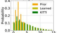
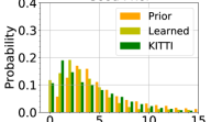


Distribution similarity metrics: In generative modeling of images, the Frechet Inception Distance [27], and the Kernel Inception Distance [5] have been used to measure progress. We report FID and KID in Tab. 2, 2 between our generated synthetic dataset and the KITTI-train set. We do so by generating 10K synthetic samples and using the full KITTI-train set, computed using the pool-3 features of an Inception-v3 network. Fig. 10 (left) shows the distribution of the number of cars generated by the prior, learnt model and in the KITTI dataset (since we have GT for cars). We do not have ground truth for which KITTI scenes could be classified into rural/suburban/urban, so we compare against the global distribution of the whole dataset. We notice that the model bridges the gap between this particular distribution well after training.
Task Performance: We report average precision for detection at 0.5 IoU i.e. AP@0.5 (following [30]) of an object detector trained to convergence on our synthetic data and tested on the KITTI validation set. We use the detection head from Mask-RCNN [25] with a Resnet-50-FPN backbone initialized with pre-trained ImageNet weights as our object detector. The task network in each result row of Tab. 2 is finetuned from the snapshot of the previous row. [30] show results with adding Image-to-Image translation to the generated images to reduce the appearance gap and results with training on a small amount of real data. We omit those experiments here and refer the reader to their paper for a sketch of expected results in these settings. Training this model directly on the full KITTI training set obtains AP@0.5 of , and , denoting a large sim-to-real performance gap left to bridge.
Using a simple prior: The priors on the structure in the previous experiments were taken from [48]. These priors already involved some human intervention, which we aim to minimize. Therefore, we repeat the experiments above with a very simple and quick to create prior on the scene structure, where a few instances of each kind of object (car, house etc.) is placed in the scene (see Fig. 11 (Left)). [30] requires a decently crafted structure prior to train the parameter network. Thus, we use the prior parameters while training our structure generator in this experiment (showing the robustness of training with randomized prior parameters), and learn the parameter network later (Tab. 2). Fig. 10 (right) shows that the method learned the distribution of the number of cars well (unsupervised), even when initialized from a bad prior. Notice that the FID/KID of the learnt model from the simple prior in Tab. 2 is comparable to that trained from a tuned prior in Tab. 2, which we believe is an exciting result.
Discussion: We noticed that our method worked better when initialized with more spread out priors than more localized priors (Tab. 2, 2, Fig. 10) We hypothesize this is due to the distribution matching metric we use being the the reverse-KL divergence between the generated and real data (feature) distributions, which is mode-seeking instead of being mode-covering. Therefore, an initialization with a narrow distribution around one of the modes has low incentive to move away from it, hampering learning. Even then, we see a significant improvement in performance when starting from a peaky prior as shown in Tab. 2. We also note the importance of pre-training the task network. Rows in Tab. 2 and Tab. 2 were finetuned from the checkpoint of the previous row. The first row (Prob. Grammar) is a form of Domain Randomization [62, 48], which has been shown to be crucial for sim-to-real adaptation. Our method, in essence, reduces the randomization in the generated scenes (by learning to generate scenes similar to the target data), and we observe that progressively training the task network with our (more specialized) generated data improves its performance. [1, 66] show the opposite behavior, where increasing randomization (or environment difficulty) through task training results in improved performance. A detailed analysis of this phenomemon is beyond the current scope and is left for future work.
5 Conclusion
We introduced an approach to unsupervised learning of a generative model of synthetic scene structures by optimizing for visual similarity to the real data. Inferring scene structures is known to be notoriously hard even when annotations are provided. Our method is able to perform the generative side of it without any ground truth information. Experiments on two toy and one real dataset showcase the ability of our model to learn a plausible posterior over scene structures, significantly improving over manually designed priors. Our current method needs to optimize for both the scene structure and parameters of a synthetic scene generator in order to produce good results. This process has many moving parts and is generally cumbersome to make work in a new application scenario. Doing so, such as learning the grammar itself, requires further investigation, and opens an exciting direction for future work.
Acknowledgement: We would like to acknowledge contributions through helpful discussions and technical support from Frank Cheng, Eric Cameracci, Marc Law, Aayush Prakash and Rev Lebaredian.
6 Supplementary Material
In the Supplementary Material, we present all experimental details in Sec. 6.1 and show additional qualitative results in Sec. 6.2.
6.1 Experimental Details
6.1.1 Loss gradient scale
We estimate the log ratio using kernel density estimators. The magnitude of this value can be large and lead to unstable training. We scale this value by . This was chosen empirically in order to match the magnitude of the MMD. Since we have in our original loss and is independent of and dependent only on the structure generation model we rewrite the loss gradient as
where is the rejection rate (rejections per successful sample) of the model when sampling the images in the batch.
6.1.2 Multi-MNIST
Feature Network Architecture: We use a ResNet architecture consisting of 6 residual blocks and 3 fully connected layers. We use the standard residual block consisting of two 3x3 convolutions with batch normalization and leaky relu activations. Average pooling is performed before passing the output to the fully connected layers. The final fully-connected layer outputs a vector of dimension 10 which corresponding to the logits for detecting whether a given digit class is in the scene. Since the Multi-MNIST images are grayscale, we duplicate them across channels to create a 3-channel image. The Multi-MNIST images are 256x256. The features used for training our structure generation model come from the average pool layer and the first two fully connected layers.
Structure Generation Model Architecture: The logits used for sampling are generated in an autoregressive fashion using an LSTM. The input of the LSTM is a one-hot encoding of the previous rule index (70 dimensional, in the Multi-MNIST case). We used a hidden dimension of 50 for the LSTM. The embedding of the one-hot encodings are computing using a fully connected layer. The output of the LSTM is produced by a fully connected layer which takes the hidden state of the LSTM as input and produces the logits used for rule sampling.
Feature Network Training: We first sample 5000 prior structures and their corresponding images, then train our feature network until we reach 75% accuracy on digit detections (around 10 epochs). We use the sigmoid cross entropy loss, and use the ADAM optimizer with learning rate , and with a batch size of 50.
Structure Generation Model Pre-Training: Using the 5000 prior structures generated for training the feature network, we train our structure generation model to minimize the negative log likelihood of the generated structures. This is done for 10 epochs using the ADAM optimizer with learning rate , and with a batch size of 100.
Structure Generation Model Training: We train using 5000 target images. We use a batch size of and for both the generated and real images. We train for 20 epochs. We use the ADAM optimizer with a learning rate of , and . We also use a moving average baseline with in order to reduce the variance of the REINFORCE estimator.
6.1.3 Aerial 2D
Feature Network Architecture: We use the same feature network architecture as the Multi-MNIST with the final fully connected layer producing a vector of dimension 100. This vector is then split into 4 vectors of dimension 25 which correspond to the logits for one hot encodings. The one hot encodings represent (ranging from 0 to 24) represent the total number of objects of that class (cars, roads, trees and houses) in the scene. Aerial images are 256x256. The features used for training our structure generation model come from the average pool layer and the first two fully connected layers.
Feature Network Training: We first sample 5000 prior structures and their corresponding images, then train our feature network until we reach 75% accuracy on car counting and road counting while ignoring the accuracy figures for trees and houses. Our loss function is the average of the cross entropy loss for each scene element. We use the ADAM optimizer with learning rate , and .
Structure Generation Model Pre-Training: Using the 5000 prior structures generated for training the feature network, we train our structure generation model to minimize the negative log likelihood of the generated structures. This is done for 10 epochs using the ADAM optimizer with learning rate , and with a batch size of 100.
Structure Generation Model Training: We train using 5000 target images only (no structure ground truth). We use a batch size of and for both the generated and real images. We train for 20 epochs. We use the ADAM optimizer with a learning rate of , and . We also use a moving average baseline with in order to reduce the variance of the REINFORCE estimator.
6.1.4 3D Driving Scenes
Structure Generation Model Architecture: We use the same architecture as the previous experiments except we use 3 models in conjunction with three scenarios, as defined by [48]. Each scenario has a slightly different grammar, as described below.
Scenario Grammars: Different grammars are used for each scenario following SDR. The most general is the city scenario grammar
| Street | |||
| CarsCarsMedianCarsCars | |||
| Cars | |||
| Foliage | |||
| Buildings | |||
| Sidewalk | |||
| Median |
The suburban grammar is a restriction of the city grammar, specifically having one collection of buildings in the and non-terminals.
| Street | |||
| CarsCarsMedianCarsCars | |||
| Cars | |||
| Foliage | |||
| Buildings | |||
| Sidewalk | |||
| Median |
The rural grammar is a further restriction with the addition of a shoulder instead of a sidewalk
| Street | |||
| Cars | |||
| Foliage | |||
| Median |
The Median non-terminal represents a grass or stone median that divides the left and right portions of the street. Note that the order of non-terminals in a production rule does not always reflection position on the scene but rather the order in sampling. The position of a child object within its parent is decided by its parameters, that come from either a prior or are learnt, using the method of [30].
Feature Network Architecture: We use the pool-3 layer of the inception-v3 network pre-trained on imagenet as our feature network.
Structure Generation Model Pre-Training: We sample 2000 prior structures for each scenario. We train the structure generation model of each scenario to minimize the negative log likelihood of the generated structures for the given scenario. This is done for 10 epochs using the default ADAM optimizer with a batch size of 100. We have two different priors for sampling structures. The prior from [30] and a simple prior. Both priors have the same sampling procedure but differ in terms of the distribution. In general sampling is done by sampling a random number of objects to be placed onto each container (the containers being Street, Outer, Shoulder, Sidewalk and Median). The sampling is done using a uniform distribution bounded by and which determine the minimum and maximum number of objects in the container. In both priors the objects (i.e pole, sign, bike) are sampled with equal probability with replacement from the set of allowable objects in that specific container. An additional detail is determining the number of lanes on the road and whether or not the scene has a Median container and where should it be placed in the rural and urban scenarios. In both priors the number of lanes is sampled uniformly from 1 to 4 and the probability of a road having a median is 0.5. This can be interpreted as selecting a random production rule for the Street non terminal. Where the priors differ is in their choices of for each container. In the prior from [30] the bounds are chosen to match the given scenario. For example in the rural setting there is a large bound on the number of foliage while in the urban setting it is smaller. Thus each container has a unique that is determined by the scenario. In the simple prior we restrict and for all containers in all scenarios.
Structure Generation Model Training: We use a batch size of for the real images . The real images are taken from the train split of the KITTI dataset. To produce our generated batch we sample images for each scenario . We then get KDE estimates
The gradient of the loss for a single structure generation model is given by
so the densities are calculated using the whole generated set but only use images generated by that scenario for the REINFORCE sample. We use the ADAM optimizer with learning rate , and . We train for 5 epochs and use a moving average baseline with in order to reduce the variance of the REINFORCE estimator.
Mask-RCNN Training: We train a Mask-RCNN [25]333Using code from: https://github.com/facebookresearch/maskrcnn-benchmark network on a generated training set and then test on the KITTI validation set [21]. In both the original and simple prior experiments we produce the generated image set by generating 10K samples for each experiment setting, with the scenario being chosen uniformly. For training, we render images with random saturation and contrast, which we observed to work better. Both the good prior and simple prior have 3 experiment settings which correspond to the rows of the Tab. 1 and 2. The training procedure for both experiments is the same.
First, we train on 10K samples from the probabilistic grammar. We use the ADAM optimizer with learning rate , and with a batch size of 2. We finetune every row of Tab. 1 and Tab. 2 from the previous row. For the next two rounds (corresponding to the second and third rows of Tab. 1 and 2), we use learning rates of and .
6.2 Additional Qualitative Results
We show additonal generated images for the simple prior experiment in Fig. 12. Notice how the prior images (left) are mostly empty, while our learnt generated images have a structure that matches the real images much better. We notice that our method is restricted by the quality of the grammar, and therefore cannot generate structures such as parking side lanes (Row 5 KITTI Image) or intersubsections (Row 7.11 KITTI image) etc. With more work on writing a grammar, we hope to learn much better structures to cover more scenarios. Training for data generation is still very important after the effort on making the grammar, since for different downstream domains (such as driving in different countries), the target dataset can change drastically and appropriate synthetic data must be generated, where learning can help mitigate long cycles of careful tuning of scene parameters by humans.


References
- [1] Akkaya, I., Andrychowicz, M., Chociej, M., Litwin, M., McGrew, B., Petron, A., Paino, A., Plappert, M., Powell, G., Ribas, R., et al.: Solving rubik’s cube with a robot hand. arXiv preprint arXiv:1910.07113 (2019)
- [2] Alhaija, H.A., Mustikovela, S.K., Mescheder, L., Geiger, A., Rother, C.: Augmented reality meets computer vision: Efficient data generation for urban driving scenes. International Journal of Computer Vision 126(9), 961–972 (2018)
- [3] Alvarez-Melis, D., Jaakkola, T.S.: Tree-structured decoding with doubly-recurrent neural networks (2016)
- [4] Armeni, I., He, Z.Y., Gwak, J., Zamir, A.R., Fischer, M., Malik, J., Savarese, S.: 3d scene graph: A structure for unified semantics, 3d space, and camera. In: Proceedings of the IEEE International Conference on Computer Vision (2019)
- [5] Bińkowski, M., Sutherland, D.J., Arbel, M., Gretton, A.: Demystifying mmd gans. ICLR (2018)
- [6] Brockman, G., Cheung, V., Pettersson, L., Schneider, J., Schulman, J., Tang, J., Zaremba, W.: Openai gym. In: arXiv:1606.01540 (2016)
- [7] Butler, D.J., Wulff, J., Stanley, G.B., Black, M.J.: A naturalistic open source movie for optical flow evaluation. In: A. Fitzgibbon et al. (Eds.) (ed.) ECCV. pp. 611–625. Part IV, LNCS 7577, Springer-Verlag (2012)
- [8] Chebotar, Y., Handa, A., Makoviychuk, V., Macklin, M., Issac, J., Ratliff, N., Fox, D.: Closing the sim-to-real loop: Adapting simulation randomization with real world experience. arXiv preprint arXiv:1810.05687 (2018)
- [9] Chen, X., Liu, C., Song, D.: Tree-to-tree neural networks for program translation. In: Bengio, S., Wallach, H., Larochelle, H., Grauman, K., Cesa-Bianchi, N., Garnett, R. (eds.) Advances in Neural Information Processing Systems 31, pp. 2547–2557. Curran Associates, Inc. (2018), http://papers.nips.cc/paper/7521-tree-to-tree-neural-networks-for-program-translation.pdf
- [10] Chu, H., Li, D., Acuna, D., Kar, A., Shugrina, M., Wei, X., Liu, M.Y., Torralba, A., Fidler, S.: Neural turtle graphics for modeling city road layouts. In: Proceedings of the IEEE International Conference on Computer Vision. pp. 4522–4530 (2019)
- [11] Cranmer, K., Brehmer, J., Louppe, G.: The frontier of simulation-based inference. arXiv preprint arXiv:1911.01429 (2019)
- [12] Dai, H., Tian, Y., Dai, B., Skiena, S., Song, L.: Syntax-directed variational autoencoder for structured data. arXiv preprint arXiv:1802.08786 (2018)
- [13] Deng, J., Dong, W., Socher, R., Li, L.J., Li, K., Fei-Fei, L.: Imagenet: A large-scale hierarchical image database. In: 2009 IEEE conference on computer vision and pattern recognition. pp. 248–255. Ieee (2009)
- [14] Dosovitskiy, A., Ros, G., Codevilla, F., Lopez, A., Koltun, V.: CARLA: An open urban driving simulator. In: CORL. pp. 1–16 (2017)
- [15] Dziugaite, G.K., Roy, D.M., Ghahramani, Z.: Training generative neural networks via maximum mean discrepancy optimization. In: UAI (2015)
- [16] Eslami, S.A., Heess, N., Weber, T., Tassa, Y., Szepesvari, D., Hinton, G.E., et al.: Attend, infer, repeat: Fast scene understanding with generative models. In: Advances in Neural Information Processing Systems. pp. 3225–3233 (2016)
- [17] Fan, S., Huang, B.: Labeled graph generative adversarial networks. CoRR abs/1906.03220 (2019), http://arxiv.org/abs/1906.03220
- [18] Gaidon, A., Wang, Q., Cabon, Y., Vig, E.: Virtual worlds as proxy for multi-object tracking analysis. In: CVPR (2016)
- [19] Ganin, Y., Kulkarni, T., Babuschkin, I., Eslami, S., Vinyals, O.: Synthesizing programs for images using reinforced adversarial learning. arXiv preprint arXiv:1804.01118 (2018)
- [20] Gao, X., Gong, R., Shu, T., Xie, X., Wang, S., Zhu, S.: Vrkitchen: an interactive 3d virtual environment for task-oriented learning. arXiv abs/1903.05757 (2019)
- [21] Geiger, A., Lenz, P., Urtasun, R.: Are we ready for Autonomous Driving? The KITTI Vision Benchmark Suite. In: CVPR (2012)
- [22] Goodfellow, I., Pouget-Abadie, J., Mirza, M., Xu, B., Warde-Farley, D., Ozair, S., Courville, A., Bengio, Y.: Generative adversarial nets. In: NIPS (2014)
- [23] Gretton, A., Borgwardt, K.M., Rasch, M.J., Schölkopf, B., Smola, A.: A kernel two-sample test. JMLR (2012)
- [24] Handa, A., Patraucean, V., Badrinarayanan, V., Stent, S., Cipolla, R.: Understanding real world indoor scenes with synthetic data. In: Proceedings of the IEEE Conference on Computer Vision and Pattern Recognition. pp. 4077–4085 (2016)
- [25] He, K., Gkioxari, G., Dollár, P., Girshick, R.: Mask r-cnn. In: Proceedings of the IEEE international conference on computer vision. pp. 2961–2969 (2017)
- [26] He, K., Zhang, X., Ren, S., Sun, J.: Deep residual learning for image recognition. CoRR abs/1512.03385 (2015), http://arxiv.org/abs/1512.03385
- [27] Heusel, M., Ramsauer, H., Unterthiner, T., Nessler, B., Hochreiter, S.: Gans trained by a two time-scale update rule converge to a local nash equilibrium. In: Advances in Neural Information Processing Systems. pp. 6626–6637 (2017)
- [28] Juliani, A., Berges, V.P., Vckay, E., Gao, Y., Henry, H., Mattar, M., Lange, D.: Unity: A general platform for intelligent agents. arXiv preprint arXiv:1809.02627 (2018)
- [29] Jyothi, A.A., Durand, T., He, J., Sigal, L., Mori, G.: Layoutvae: Stochastic scene layout generation from a label set. In: The IEEE International Conference on Computer Vision (ICCV) (October 2019)
- [30] Kar, A., Prakash, A., Liu, M.Y., Cameracci, E., Yuan, J., Rusiniak, M., Acuna, D., Torralba, A., Fidler, S.: Meta-sim: Learning to generate synthetic datasets. In: ICCV (2019)
- [31] Karras, T., Laine, S., Aila, T.: A style-based generator architecture for generative adversarial networks. arXiv preprint arXiv:1812.04948 (2018)
- [32] Kim, Y., Dyer, C., Rush, A.M.: Compound probabilistic context-free grammars for grammar induction. vol. abs/1906.10225 (2019), http://arxiv.org/abs/1906.10225
- [33] Kingma, D.P., Welling, M.: Auto-encoding variational bayes. arXiv preprint arXiv:1312.6114 (2013)
- [34] Kolve, E., Mottaghi, R., Gordon, D., Zhu, Y., Gupta, A., Farhadi, A.: Ai2-thor: An interactive 3d environment for visual ai. In: arXiv:1712.05474 (2017)
- [35] Kulkarni, T.D., Kohli, P., Tenenbaum, J.B., Mansinghka, V.: Picture: A probabilistic programming language for scene perception. In: Proceedings of the ieee conference on computer vision and pattern recognition. pp. 4390–4399 (2015)
- [36] Kulkarni, T.D., Whitney, W.F., Kohli, P., Tenenbaum, J.: Deep convolutional inverse graphics network. In: NIPS. pp. 2539–2547 (2015)
- [37] Kusner, M.J., Paige, B., Hernández-Lobato, J.M.: Grammar variational autoencoder. In: Proceedings of the 34th International Conference on Machine Learning - Volume 70. pp. 1945–1954. ICML’17, JMLR.org (2017), http://dl.acm.org/citation.cfm?id=3305381.3305582
- [38] LeCun, Y.: The mnist database of handwritten digits. http://yann. lecun. com/exdb/mnist/
- [39] Li, C.L., Chang, W.C., Cheng, Y., Yang, Y., Póczos, B.: Mmd gan: Towards deeper understanding of moment matching network. In: NIPS (2017)
- [40] Li, M., Patil, A.G., Xu, K., Chaudhuri, S., Khan, O., Shamir, A., Tu, C., Chen, B., Cohen-Or, D., Zhang, H.: Grains: Generative recursive autoencoders for indoor scenes. ACM Transactions on Graphics (TOG) 38(2), 12 (2019)
- [41] Li, Y., Swersky, K., Zemel, R.: Generative moment matching networks. In: ICML (2015)
- [42] Li, Y., Vinyals, O., Dyer, C., Pascanu, R., Battaglia, P.: Learning deep generative models of graphs. arXiv preprint arXiv:1803.03324 (2018)
- [43] Liao, R., Li, Y., Song, Y., Wang, S., Nash, C., Hamilton, W.L., Duvenaud, D., Urtasun, R., Zemel, R.S.: Efficient graph generation with graph recurrent attention networks. arXiv preprint arXiv:1910.00760 (2019)
- [44] Louppe, G., Cranmer, K.: Adversarial variational optimization of non-differentiable simulators. arXiv preprint arXiv:1707.07113 (2017)
- [45] Mansinghka, V.K., Kulkarni, T.D., Perov, Y.N., Tenenbaum, J.: Approximate bayesian image interpretation using generative probabilistic graphics programs. In: Advances in Neural Information Processing Systems. pp. 1520–1528 (2013)
- [46] McCormac, J., Handa, A., Leutenegger, S., Davison, A.J.: Scenenet rgb-d: 5m photorealistic images of synthetic indoor trajectories with ground truth. arXiv preprint arXiv:1612.05079 (2016)
- [47] Mellor, J.F.J., Park, E., Ganin, Y., Babuschkin, I., Kulkarni, T., Rosenbaum, D., Ballard, A., Weber, T., Vinyals, O., Eslami, S.M.A.: Unsupervised doodling and painting with improved spiral (2019)
- [48] Prakash, A., Boochoon, S., Brophy, M., Acuna, D., Cameracci, E., State, G., Shapira, O., Birchfield, S.: Structured domain randomization: Bridging the reality gap by context-aware synthetic data. In: arXiv:1810.10093 (2018)
- [49] Puig, X., Ra, K., Boben, M., Li, J., Wang, T., Fidler, S., Torralba, A.: Virtualhome: Simulating household activities via programs. In: CVPR (2018)
- [50] Qi, S., Zhu, Y., Huang, S., Jiang, C., Zhu, S.C.: Human-centric indoor scene synthesis using stochastic grammar. In: Proceedings of the IEEE Conference on Computer Vision and Pattern Recognition. pp. 5899–5908 (2018)
- [51] Razavi, A., Oord, A.v.d., Vinyals, O.: Generating diverse high-fidelity images with vq-vae-2. arXiv preprint arXiv:1906.00446 (2019)
- [52] Rezende, D.J., Mohamed, S., Wierstra, D.: Stochastic backpropagation and approximate inference in deep generative models. arXiv preprint arXiv:1401.4082 (2014)
- [53] Richter, S.R., Vineet, V., Roth, S., Koltun, V.: Playing for data: Ground truth from computer games. In: ECCV (2016)
- [54] Ritchie, D., Wang, K., Lin, Y.A.: Fast and flexible indoor scene synthesis via deep convolutional generative models. In: The IEEE Conference on Computer Vision and Pattern Recognition (CVPR) (June 2019)
- [55] Ros, G., Sellart, L., Materzynska, J., Vazquez, D., Lopez, A.: The SYNTHIA Dataset: A large collection of synthetic images for semantic segmentation of urban scenes. In: CVPR (2016)
- [56] Sadeghi, F., Levine, S.: Cad2rl: Real single-image flight without a single real image. arXiv preprint arXiv:1611.04201 (2016)
- [57] Savva, M., Kadian, A., Maksymets, O., Zhao, Y., Wijmans, E., Jain, B., Straub, J., Liu, J., Koltun, V., Malik, J., et al.: Habitat: A platform for embodied ai research. arXiv preprint arXiv:1904.01201 (2019)
- [58] Shugrina, M., Liang, Z., Kar, A., Li, J., Singh, A., Singh, K., Fidler, S.: Creative flow+ dataset. In: Proceedings of the IEEE Conference on Computer Vision and Pattern Recognition. pp. 5384–5393 (2019)
- [59] Song, S., Yu, F., Zeng, A., Chang, A.X., Savva, M., Funkhouser, T.: Semantic scene completion from a single depth image. Proceedings of 30th IEEE Conference on Computer Vision and Pattern Recognition (2017)
- [60] Such, F.P., Rawal, A., Lehman, J., Stanley, K.O., Clune, J.: Generative teaching networks: Accelerating neural architecture search by learning to generate synthetic training data. arXiv preprint arXiv:1912.07768 (2019)
- [61] Tassa, Y., Doron, Y., Muldal, A., Erez, T., Li, Y., de Las Casas, D., Budden, D., Abdolmaleki, A., Merel, J., Lefrancq, A., Lillicrap, T., Riedmiller, M.: DeepMind control suite. Tech. rep., DeepMind (Jan 2018), https://arxiv.org/abs/1801.00690
- [62] Tobin, J., Fong, R., Ray, A., Schneider, J., Zaremba, W., Abbeel, P.: Domain randomization for transferring deep neural networks from simulation to the real world. In: IROS (2017)
- [63] Todorov, E., Erez, T., Tassa, Y.: Mujoco: A physics engine for model-based control. In: Intl. Conf. on Intelligent Robots and Systems (2012)
- [64] Wang, K., Lin, Y.A., Weissmann, B., Savva, M., Chang, A.X., Ritchie, D.: Planit: Planning and instantiating indoor scenes with relation graph and spatial prior networks. ACM Transactions on Graphics (TOG) 38(4), 132 (2019)
- [65] Wang, K., Savva, M., Chang, A.X., Ritchie, D.: Deep convolutional priors for indoor scene synthesis. ACM Transactions on Graphics (TOG) 37(4), 70 (2018)
- [66] Wang, R., Lehman, J., Clune, J., Stanley, K.O.: Poet: open-ended coevolution of environments and their optimized solutions. In: Proceedings of the Genetic and Evolutionary Computation Conference. pp. 142–151 (2019)
- [67] Williams, R.J.: Simple statistical gradient-following algorithms for connectionist reinforcement learning. Machine learning (1992)
- [68] Wrenninge, M., Unger, J.: Synscapes: A photorealistic synthetic dataset for street scene parsing. In: arXiv:1810.08705 (2018)
- [69] Wu, J., Tenenbaum, J.B., Kohli, P.: Neural scene de-rendering. In: IEEE Conference on Computer Vision and Pattern Recognition (CVPR) (2017)
- [70] Wu, Y., Wu, Y., Gkioxari, G., Tiani, Y.: Building generalizable agents with a realistic and rich 3d environment. In: arXiv:1801.02209 (2018)
- [71] Yin, P., Neubig, G.: A syntactic neural model for general-purpose code generation. CoRR abs/1704.01696 (2017), http://arxiv.org/abs/1704.01696
- [72] Yin, P., Zhou, C., He, J., Neubig, G.: Structvae: Tree-structured latent variable models for semi-supervised semantic parsing. CoRR abs/1806.07832 (2018), http://arxiv.org/abs/1806.07832
- [73] You, J., Ying, R., Ren, X., Hamilton, W., Leskovec, J.: Graphrnn: Generating realistic graphs with deep auto-regressive models. In: International Conference on Machine Learning. pp. 5694–5703 (2018)
- [74] Yu, L.F., Yeung, S.K., Tang, C.K., Terzopoulos, D., Chan, T.F., Osher, S.: Make it home: automatic optimization of furniture arrangement. ACM Trans. Graph. 30(4), 86 (2011)
- [75] Zhang, Y., Song, S., Yumer, E., Savva, M., Lee, J.Y., Jin, H., Funkhouser, T.: Physically-based rendering for indoor scene understanding using convolutional neural networks. In: The IEEE Conference on Computer Vision and Pattern Recognition (CVPR) (July 2017)
- [76] Zhou, Y., While, Z., Kalogerakis, E.: Scenegraphnet: Neural message passing for 3d indoor scene augmentation. In: The IEEE International Conference on Computer Vision (ICCV) (October 2019)