Sample-efficient benchmarking of multi-photon interference on a boson sampler in the sparse regime

Abstract

Verification of a quantum advantage in the presence of noise is a key open problem in the study of near-term quantum devices. In this work, we show how to assess the quality of photonic interference in a linear optical quantum device (boson sampler) by using a maximum likelihood method to measure the strength at which various noise sources are present in the experiment. This allows us to use a sparse set of samples to test whether a given boson sampling experiment meets known upper bounds on the level of noise permissible to demonstrate a quantum advantage. Furthermore, this method allows us monitor the evolution of noise in real time, creating a valuable diagnostic tool. Finally, we observe that sources of noise in the experiment compound, meaning that the observed value of the mutual photon indistinguishability, which is the main imperfection in our study, is an effective value taking into account all sources of error in the experiment.

I Introduction

With the increasing computational power of quantum information processing devices Arute2019 ; Pino2020 ; Wang2019b , it has become a pressing problem how to demonstrate the computational advantage that a quantum device has over a classical one (also known as ’quantum supremacy’). A key issue is verification, i.e. the problem of checking that the quantum device is truly outperforming classical computer. Ideally, a quantum advantage demonstration would be arranged so that verification can be done efficiently with respect to the size of the quantum system. For example, an efficiently verifiable quantum advantage can be demonstrated on a universal, fault-tolerant computer by a fast solution to a problem such as prime factoring, i.e. one whose output can be efficiently checked, and for which a fast quantum algorithm is known but not a classical one. If the quantum machine can solve the posed problem much faster than a classical computer, this would constitute very strong evidence of the quantum nature of the device.

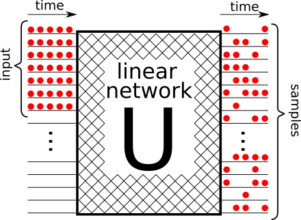
However, for the forseeable future, the main devices of experimental interest are noisy intermediate-scale quantum devices (NISQ), which are small-to-medium sized devices without quantum error correction. These devices usually work by solving a sampling problem over some probability distribution more efficiently than is believed to be possible classically Preskill2018 ; Harrow2017 . In photonics, this takes the form of sampling over the output distribution of interfering photons in a linear optical network, a problem known as boson sampling (see Figure 1) Aaronson2011 . For such devices, no problems are known which fit all three requirements for efficient verification (easy to solve on a NISQ device, hard to solve classically, easy to verify). Informally stated, the issue is that it has not proven possible to find some property to be hidden in the distribution which can be efficiently tested for quantumly but not classically. Therefore, the usual approach in proving quantum operation in such a device is a brute force one, where the operation of the device is directly reconstructed at a computational cost exponential in the system size.

A further problem in the demonstration of a quantum advantage using NISQ devices is the influence of noise, i.e. any unwanted physical effect which degrades the performance of the device. For NISQ devices, the physical picture is that noise pushes the distribution over which the device samples closer to the distribution associated with classical operation of the device Boixo2018 . For quantum advantage demonstrations based on random circuit sampling Arute2019 , it was recently proposed that if the noise pushes the system towards the uniform distribution, any level of noise which doesn’t completely revert the device to sampling over a classical distribution is sufficient to maintain a quantum advantage Aaronson2019 . However, this result relies on strong complexity-theoretic assumptions regarding the classical hardness of identifying properties of the probability distribution over which the device is sampling.

For boson sampling, in contrast, pseudoprobability distributions are known which approximate the sampling distribution in the presence of noise Renema2018a ; Renema2018b ; Shchesnovich2019a ; Shchesnovich2019b ; Moylett2019 ; Renema2019 , and from which it is believed to be possible to sample efficiently. The distance between these distributions and the output distribution of the device depends on the level of noise, and for sufficiently high levels of noise the two distributions are close, ruling out a quantum advantage in that regime.

However, the application of such classicality thresholds requires knowledge of which noise sources are present in a boson sampler, and at what strength. The main sources of noise in a boson sampler are photon loss Aaronsonweb2 , and partial distinguishability Tichypartial . So far, the level of noise in boson sampling experiments was mostly inferred by measuring the complete output distribution and comparing it to the ideal (i.e. noiseless) output distribution, where the experiment is declared a success if the distance between these is sufficiently low. However, this approach is inherently non-scalable in the number of measurements required Aaronson2011 since the probability of observing any single outcome decreases exponentially with the number of photons. The other approach was to compare the hypothesis of fully distinguishable photons with that of fully indistinguishable ones Bentivegna2014 , which does not capture the full range of possible effects in the device Tichypartial . This issue recently became pressing with the demonstration of the first boson sampler operating in the sparse regime Wang2019b , i.e. where the size of the Hilbert space makes measuring the output distribution infeasible, and only a sparse set of samples can be collected. This raises the question of how to assess the quality of quantum interference in such a system.

In this work, we show that all information required to assess the quality of quantum interference in a boson sampler is contained in just a sparse set of samples. We use a maximum likelihood method to infer the relevant properties of the photons, in particular their mutual indistinguishability. We apply this method to a sparse set of samples produced on the experimental apparatus reported in Wang2019b . There is a discrepancy between the measured indistinguishability in the sampler and that inferred from independent measurements, which we explain by demonstrating that all other imperfections result in a decrease of the indistinguishability. This value must therefore be interpreted as an effective value taking into account many sources of noise. Using this fact, we can construct an error budget for a boson sampler. We also show how to use this method to monitor the quality of photonic interference in real time, showing its use as a diagnostic tool. Our method is essentially a non-trivial extension of the Hong-Ou-Mandel interference Hong1987 to measure the mutual overlap of photons in a highly complex multi-photon, multi-mode case.

Together with the results on the permissible level of noise in a boson sampler Renema2018a ; Renema2018b ; Shchesnovich2019a ; Shchesnovich2019b ; Moylett2019 ; Renema2019 , these results solve the problem of testing whether a given boson sampling experiment passes the known requirements to exibit a quantum advantage without any additional characterization experiments besides measuring the transmission matrix of the system, which can be done efficiently Laing2012 . Our method is efficient in the number of samples required, but not efficient in the number of computations required, as is expected for a NISQ quantum advantage verification protocol.

Our work is structured as follows: we begin with a short overview of the experimental apparatus on which the samples to which we apply our method were produced. We then detail our maximum likelihood analysis method. Finally, we conduct numerical simulations to show that the effect of other imperfections is to decrease the degree of indistinguishability.

Figure 1: A sketch of a boson sampler. A series of $n$ modes out of a large linear interferometer are fed with single photons, and samples from the resulting distribution are recorded at the output.

II experimental imperfections

The experimental apparatus on which our dataset was generated consists of an InAs/GaAs quantum-dot source operating at 893 nm pumped with a pulsed laser with 1.2 nW intensity and a repetition rate of 76 MHz, corresponding to a pulse energy of $1.6\times 10^{-17}\$J. This single-photon source is then demultiplexed using a tree of 19 Pockels cells, and fed into a fixed free-space interferometer with 60 optical modes, where quantum interference occurs. Finally, detection is done by a bank of superconducting single-photon detectors which are fiber-coupled to these modes. Samples consist of the set of detectors which are triggered in each run of the experiment, and are recorded using standard correlation electronics. More details of the setup are provided in Wang2019b .

The dataset under consideration here consists of lists of samples from this device. For simplicity of the analysis, postselection was used to focus on those samples where the number of photons incident is equal to the number of detection events reported, thereby removing the effect of photon loss from consideration. The number of detected photons varied between $n=3$ and $n=7$, with the length of the list of samples varying from 161 at $n=6$ to $3\times 10^{4}$ at $n=3$. Besides the samples, the dataset also contains the transmission matrix $M$ of the interferometer, which was characterized independently. A further restriction on the list of samples is given by the threshold nature of the single-photon detectors combined with postselection, namely that all samples must be collision-free in order to be registered, i.e. all $n$ photons must emerge from distinct output modes.

This experimental setup contains four imperfections of note, which result in samples which do not correspond to ideal $n$-photon quantum transmission in the interferometer. First: the generated photons are not perfectly indistinguishable, which is a requirement for maximally strong quantum interference. Second, the input states occasionally contain additional noise photons. This results in samples where one single photon is lost, but where this is compensated by one of the modes containing two photons instead, preserving the total photon number. Third, the detectors in the system produce dark counts (false positives), resulting in events where one photon is lost and replaced by a dark count. Finally, there is uncertainty in measuring the transmission matrix $M$, resulting in differences between the actual and expected interference patterns.

III Photon distinguishability

To measure the strength of these imperfections, we use a standard maximum likelihood approach. We will begin by considering only indistinguishability, adding in the other imperfections later.

The intuition behind the maximum likelihood method is that if we have some probability distribution $p$, which is a function of a set of parameters $\theta,$ we can estimate $\theta$ from a list of samples by the following expression: $\theta_{ml}=\mathrm{argmax_{\theta}}(\Lambda(\theta)),$ with $\Lambda(\theta)=\prod_{i}p_{i}(\theta)$ i.e. we must maximize with respect to $\theta$ the total likelihood to find the observed series of samples. Under relatively benign mathematical assumptions, such as continuity of the likelihood function, this is an unbiased and optimal way of estimating $\theta$.

Figure 2: The effect of partial photon distinguishability $x$ on the probability for 10 randomly chosen output configurations. Inset: Monte Carlo estimate of the correction factor arising from the restriction of our dataset to collisionless samples.

We will begin by focussing only on the effect of partial distinguishability. In a boson sampler operating at some level of partial distinguishability, the probability of a given outcome can be written as Shchesnovich2014 ; Shchesnovich2015a ; Shchesnovich2015b :

$$P(X)=\sum_{\sigma\in S_{n}}\left(\prod_{j}S_{j,\sigma_{j}}\right)\mathrm{Perm}(M\circ M_{\sigma,1}^{\dagger}),$$ (1)

where $S$ is a matrix of distinguishabilities defined elementwise as $S_{ij}=\langle x_{i}|x_{j}\rangle,$ $|x\rangle_{i}$ is the internal wave function of the $i$-th photon, $\mathrm{Perm}$ is the permanent function, $\sigma$ is a permutation of size $n,$ indices on matrices denote permutation according to those indices, and $M$ is the submatrix of $U$ connecting the modes containing an input photon to the outputs of interest Scheel2008 , and $\circ$ is the elementwise product.

It is this matrix $S$ which we are interested in estimating. Throughout this work, we will parametrize $S$ elementwise as $S_{ij}=x+(1-x)\delta_{ij},$ i.e. we assume that all pairs of photons have equal overlap with each other, which we can then set to be real without loss of generality. We will show in the Supplemental Material that it is an appropriate appropriate parametrization of $S$ for our experimental data. Note that in this parametrization $P(x)$ is a polynomial of degree $n$ in $x$ Rohde2015 .

A complication arises because we are sampling over the subset of collision-free events due to the threshold nature of the detector. This means that we must assign probability $0$ to events containing a collision, and increase the probability of noncollision events by a factor $C,$ where $C(x)=1/\sum_{i}P_{i}(x)$ is the normalization factor obtained by summing all non-collision events. Inconveniently, the total probability of obtaining a non-collision event depends on the level of indistinguishability, meaning that $C(x)$ must estimated as well. We estimate $C(x)$ using a Monte Carlo procedure, sampling uniformly over $10^{4}$ possible output modes.

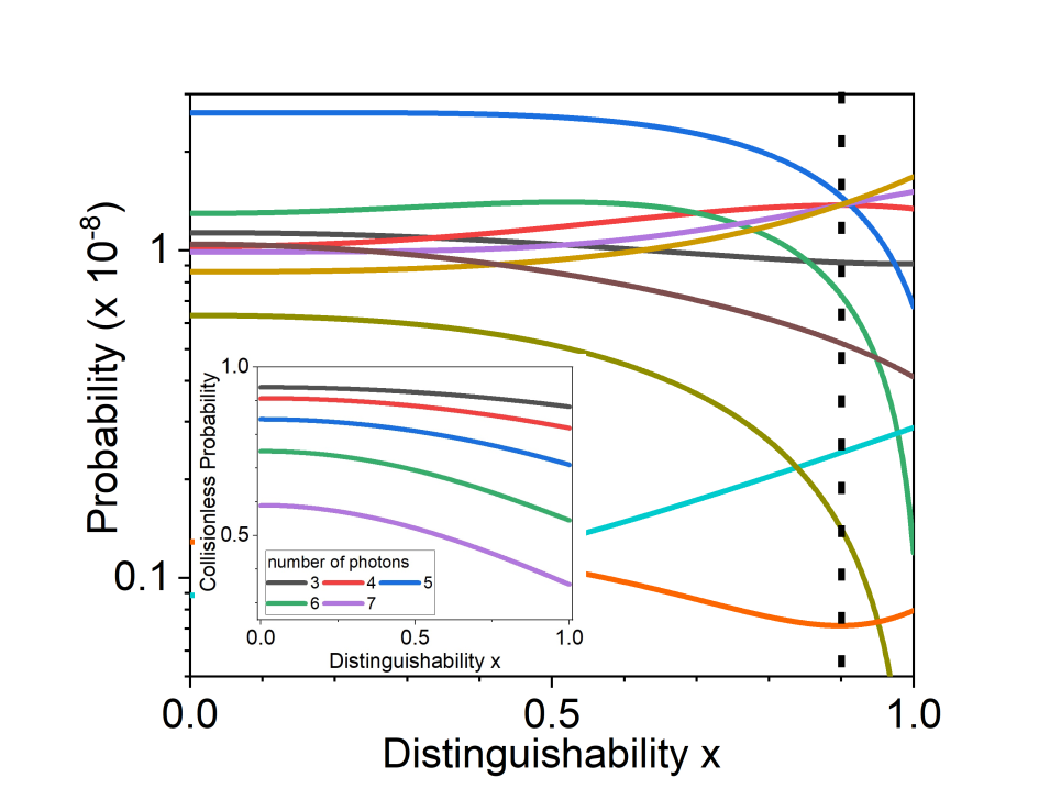
Figure 2 illustrates the intuition behind the ML approach for boson sampling. The main figure shows ten arbitrarily chosen samples from our experiment, for $n=7,$ as a function of the level of mutual indistinguishability $x.$ It can be observed that the output probability for each event is a function of the level of imperfections in the system, and that these probabilities are not monotonic in $x$. By noting which samples we have observed, we can obtain information about the level of indistinguishability at which our sampler is operating.

The inset shows our Monte Carlo estimate of the fraction of collision events (i.e. $1-C(x))$. Note that since the photon number increases while the number of modes remains constant, the probability of a collision event goes up strongly as a function of photon number. Having estimated the correction factor due to collision events and computed each output probability as a function of the level of mutual indistinguishability, we can now maximize the likelihood function to obtain an estimate for $x.$

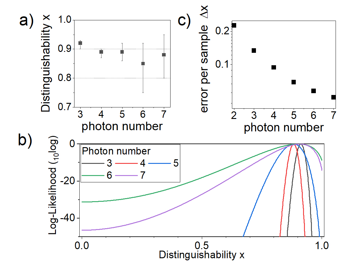
Figure 3a shows the results our estimation. We compute that across all our experiments, our photons have a mean wavefunction overlap of $x=0.89\pm 0.02,$ as shown by the black points in Fig. 3a, corresponding to a HOM dip depth of $x^{2}=0.79$. The error bars in Fig. 3a are given by the point where the relative likelihood is smaller than 0.05. Fig. 3b shows the likelihood functions evaluated from $0<x<1.$ Note that for all $n,$ $\Lambda(x=1)\gg\Lambda(x=0),$ which explains why the effect of partial distinguishability was not detected by previous tests, which compared only fully distinguishable and fully indistinguishable photons Wang2019b , or combinations of such Bentivegna2014 , as was noted previously by Dai2020 .

Figure 3c shows an estimate of the accuracy of our method, as a function of photon number. The variation in the size of the error bars in figure 3a) is mainly attributable to the vastly differing numbers of samples. To get an estimate of the efficiency per sample, we numerically simulate processing 10000 samples of each photon number at $x=1,$ and compute the resulting uncertainty in estimating $x$ by looking at the relative likelihood. We find that the error of our method decreases with the number of photons. The intuition behind this is that since the indistinguishability is a polynomial of degree $n$ in $x$ Renema2018a , increasing the number of photons increases the changes in probability around the maximum of the likelihood function.

Figure 3: a) Maximum likelihood estimation of the partial distinguishability $x=\langle\psi_{i}|\psi_{j}\rangle,$ from a sparse series of samples. b) Log-likelihood functions plotted between $0\leq x\leq 1.$ The colours indicate the number of photons. c) numerical simulation of the accuracy of our experiment, normalized to a constant number of samples.

IV Role of other imperfections

Figure 3 raises an important question: if the wavefunction overlap between our photons is approximately $x=0.89\pm 0.02$, why does an independent measurement of the overlap between our photons via the Hong-Ou-Mandel effect measure $x=0.981$ Wang2017 ? The answer to this question is that imperfections in boson sampling compound one another, resulting in a reduction of the effective photon distinguishability. This was shown explicitly for indistinguishability and loss Renema2018b , as well as for indistinguishability and noise on the matrix $M$ Shchesnovich2019a . In both of these cases, the physical picture is that noise sources affect the interference pattern in similar ways, and can therefore be thought of as strengthening one another. Therefore, we must look to the other noise sources in our experiment (dark counts, multiphoton emission, and misspecification of $M)$ to explain the discrepancy between our inferred $x$ and that observed from HOM measurements.

To demonstrate this physical mechanism, we have performed a full numerical simulation of our experiment, for $n=3.$ The procedure is as follows: we generate a set of samples which contains all the same imperfections as our real experiment, at the strengths at which we have measured them to be present in the experiment from independent characterization experiments. We then analyse these samples using the same procedure which we used to analyse the actual experimental data, and report on the observed value of $x.$

To generate these samples, we use a Markov Chain Monte Carlo sampling routine, adapted from Neville2017 . Details are provided in the Supplemental Material. We account for dark counts by adding some samples with $n=2$ among all three possible combinations of pairs of input modes, and generating the third detection event according to the measured dark count rate of our detectors. We account for multiphoton emission by generating samples from all nine combinations of states containing two of the wanted photons and one noise photon. We account for misspecification (measurement error) on the independent measurement of the interferometer by perturbing our observed interferometer $M$ with elementwise Gaussian noise. We assess the strength of each of these noise sources independently from separate calibration experiments : a $3$% probability of a dark count, a $1.2$% probability of double photon emission per mode, and approximately $1\%$ error on measuring the elements of $M.$

Table 1 shows the impact of these noise sources. By performing a series of simulations where we switch these imperfections on one at a time, and reconstructing $x$ at each step, we can get an idea of the cumulative impact which each of these imperfections has on our boson sampler. Table 1 can therefore also be interpreted as an error budget for our boson sampler, in that it shows which imperfections most reduce the level of indistinguishability. In particular, the effect of multiphoton states is almost a factor 4 larger than that of misspecification of M and of dark counts, but of the same order as the reduction of $x$ due to true indistinguishability. This shows that the main challenges in improving the quantumness of our boson sampler lie in improving the quantum dot source.

Imperfection	Value of $x$ inferred	10log$\left(\Lambda_{s}/\Lambda_{e}\right)$
$x$ from HOM experiment	0.981 $\pm$ 0.002	-130
Misspecification of $M$	0.970 $\pm$ 0.008	-83
Multiphoton states	0.924 $\pm$ 0.009	-2.5
Dark counts	0.913 $\pm$ 0.010	0

Table 1: Error budget for a boson sampler. The first column shows the value of the indistinguishability when that particular imperfection and the ones above it in the table are applied. The second column shows the relative likelihood of the corresponding value of $x$ as derived from the simulation, normalized to the maximum value of the likelihood function derived from the experimental data.

To compare our simulation to our experimental data, we also report in Table 1 the relative likelihood of the value of $x$ (expressed as its 10-log) from our simulations ($\Lambda_{s})$ relative to the likelihood derived from our expeirmental data ($\Lambda_{e})$. This shows that when we ‘switch on’ all imperfections, our simulation predicts a value of $x$ within the error bar of the one which we measure in our experiment, and hence that our simulation and our measurement are consistent. This validates the picture of our inferred maximum likelihood indistinguishability value being essentially an effective value that takes into account all other known sources of error in the experiment.

V Real-time monitoring

A practical application of our result is that we can monitor the strength of the noise sources in our experiment in real time, by making use of a rolling average. In this way, we can detect changes in the noise parameters of our experiment in real time, opening up a valuable diagnostic tool for stabilizing an experimental boson sampling setup.

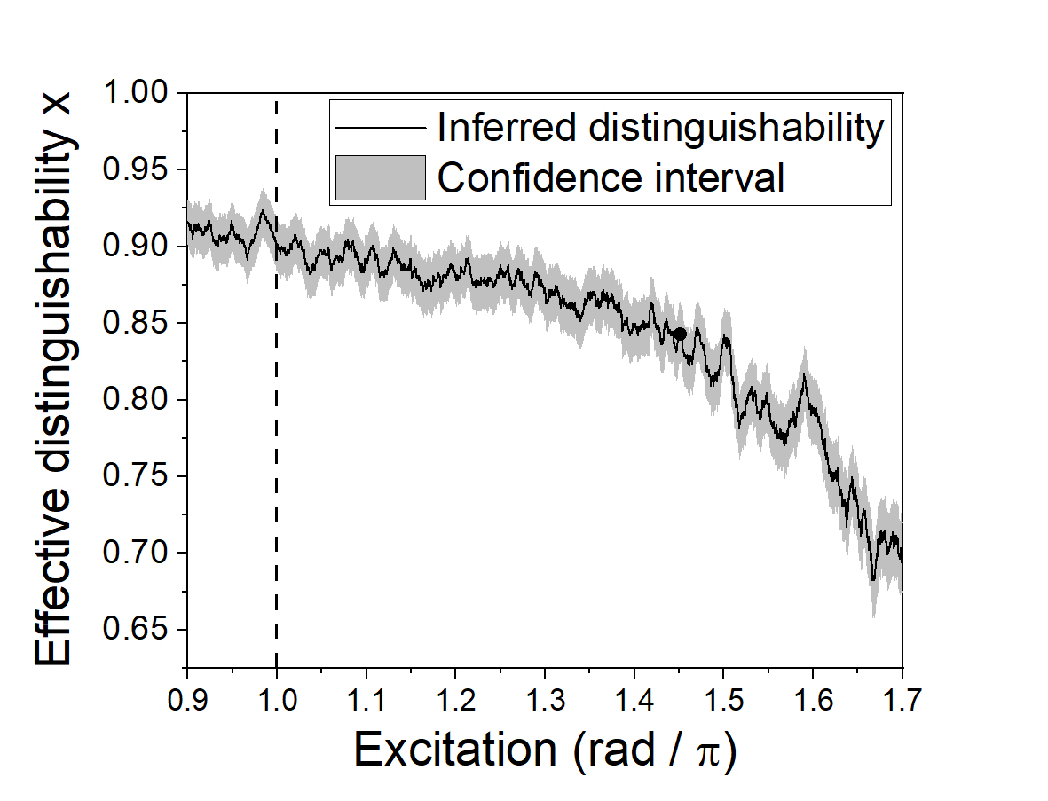
To illustrate this procedure, Figure 4 shows a case in which we have artificially increased the $g^{(2)}$ of our photon source by increasing the excitation power of the pump pulse from $1.19\times 10^{-17}$ mJ to $4.58\times 10^{-17}$ mJ. To obtain the $i$-th point in this graph, we compute the maximum likelihood estimate of the $i$-th to $i+10000$-th consecutive samples from the experiment. The resulting estimate shows a clear continuous decrease in the effective photon indistinguishability, demonstrating the use of this method for real-time monitoring.

Figure 4: Real time monitoring of the effective degree of photon indistinguishability in a boson sampler as a function of excitation power. To decrease the effective degree of indistinguishability, the pump power on the quantum dot single photon source was increased to push the exitation away from the ideal $\pi$-pulse (indicated with a dashed line). The black curve shows a rolling avergae estimate of $x,$ averaging over 10.000 consecutive samples, with the grey band showing the 95% confidence interval.

VI Discussion & Conclusion

An important restriction in our approach is that Equation 1 is expensive to evaluate, since it requires the computation of $n!$ many permanents, each of which comes at a cost of $n2^{n}$ computational steps. This can be reduced to $2n2^{2n}$ by applying a multidimensional extension to Ryser’s formula Tichypartial , but this still restricts application of this approach to approximately 25 photons Wusupercomputer . Two approaches are possible: either to use the approximate probabilities of Renema2018a ; Renema2018b ; Shchesnovich2019a ; Shchesnovich2019b ; Moylett2019 ; Renema2019 , or to use simpler circuits for the measurement of $x,$ as was done in the benchmarking of Google’s random circuit sampling experiment Arute2019 . We leave the issue of finding the appropriate circuits for the photonic case as an open problem for future work. Another further extension of this work would be to strengthen our belief in the thresholds for classicality by teing them to a complexity conjecture, as was done for random circuit sampling Aaronson2019 .

In conclusion, we have demonstrated how to infer the quality of a boson sampler from a sparse series of samples. We have demonstrated that the measured indistinguishability is an effective value, which accounts for a series of imperfections. These results show how to demonstrate that a candidate quantum advantage demonstration using photonics outperforms the best known simulation algorithms.