Numerical solutions to Giovannini’s parton branching equation up to TeV energies at the LHC

Abstract

Giovannini’s parton branching equation is integrated numerically using the 4^th-order Runge-Kutta method. Using a simple hadronisation model, a charged-hadron multiplicity distribution is obtained. This model is then fitted to various experimental data up to the TeV scale to study how the Giovannini parameters vary with collision energy and type. The model is able to describe hadronic collisions up to the TeV scale and reveals the emergence of gluonic activity as the centre-of-mass energy increases. A prediction is made for $\sqrt{s}$ = 14 TeV.

1 Introduction

The charged particle multiplicity distribution is one of the important primary measurements made at every high energy physics collision experiment. Particle physics phenomenology attempts to create models to describe the observed multiplicity distributions, and distributions such as the Negative Binomial Distribution (NBD) and Generalised Multiplicity Distribution (GMD) Chan1990 have been very successful in describing observed data, at least up to the emergence of KNO scaling violation reported by the UA5 collaboration in the 1980s Alner1986 . The appearance of a “shoulder-like structure” hinted at a new process that was taking place, and the common approach by phenomenologists since then was to fit the observations to a multi-component distribution. For example, a two-component distribution can be composed as:

$$\begin{split}P(n;\overline{n},k,\overline{n}^{\prime},k^{\prime})=&\alpha P_{\text{NBD}}(n;\overline{n},k)\\ &+(1-\alpha)P_{\text{NBD}}^{\prime}(n;\overline{n}^{\prime},k^{\prime})\end{split}$$ (1)

where the resultant distribution $P(n)$ is a weighted sum of two individual distributions, each with its own set of parameters (see for example ref. Ghosh2012c , where the two components describe “soft” and “semihard” events). Three-component distributions have also been explored as a possible explanation to other observed phenomena in multiplicity distributions such as oscillations of combinants Zborovsky2018 .

Distributions such as the NBD and GMD are partial solutions to Giovannini’s parton branching equation Giovannini1979 (henceforth “Giovannini’s equation”) which describes multiparticle production within the framework of perturbative QCD (pQCD). For $m$ quarks and $n$ gluons at QCD evolution parameter $t$, we have:

$$\begin{split}\frac{\partial P_{m,n}}{\partial t}=&-(An+\widetilde{A}m+Bn+Cn)P_{m,n}\\ &+A(n-1)P_{m,n-1}\\ &+\widetilde{A}mP_{m,n-1}\\ &+B(n+1)P_{m-2,n+1}\\ &+C(n-2)P_{m,n-2}\end{split}$$ (2)

where $A$, $\widetilde{A}$, $B$ and $C$ (henceforth the “Giovannini parameters”) are the probabilities of the processes

$$\begin{split}&A:g\rightarrow gg\;&&\text{(gluon bremsstrahlung)}\\ &\widetilde{A}:q\rightarrow qg&&\text{(quark bremsstrahlung)}\\ &B:g\rightarrow q\overline{q}&&\text{(quark pair creation)}\\ &C:g\rightarrow ggg&&\text{(four-gluon vertex)}\end{split}$$ (3)

taking place. The GMD is a partial solution to the parton branching equation for the special case $B=C=0$, and the NBD is a special case of the GMD where $k^{\prime}=0$. It must be noted then, that these solutions do not capture all the processes considered by Giovannini.

At the point of writing, a full analytic distribution incorporating all four of Giovannini’s processes does not exist. However, several attempts at a partial solution have been studied and made, for example by Biyajima, Suzuki and Wilk Biyajima1983 ; Biyajima1984b ; Biyajima1984 ; Biyajima1984a ; Biyajima1988b ; Suzuki1991 , Carruthers and Shih Shih1986 ; Carruthers1987 , Durand and Sarcevic Durand1986 ; Durand1987 , Sakai Sakai1989 , Gupta and Sarma Gupta1991 , Hwa Hwa1988 and Chan and Chew Chan1992b . Since an exact solution is difficult to obtain, we look to numerical methods. Of interest to this work is Sakai’s attempt at a numerical solution Sakai1989 ; in it, the $C$-process was omitted (and hence a full solution to eq. (2) was not explored) and best-fit parameters to experimental data were not reported. However, oscillations were present in the hadron multiplicity plots generated (Figures 1(b) and 1(c) in Sakai1989 ), which are of interest and might be relevant to the shoulder-like structure observed in KNO scaling violation.

Hence, with newer data available in the TeV-era of the LHC, we reattempt to construct a “single-component distribution” numerical model to see if it can better describe charged-particle multiplicity distributions, well into the KNO scaling violation regime up to the TeV scale.

This article is organised as follows. Section 2 outlines our numerical model, where the procedure from integrating Giovannini’s parton branching equation to applying a hadronisation model to produce the final charged-particle multiplicity distribution is detailed. Section 3 explores some properties of the model parameters and how they affect the final multiplicity distribution. Section 4 outlines the fitting procedure used to fit against data and the results, followed by a discussion about it in section 5. In section 6 we make a prediction for higher energies, and we end in section 7 with some concluding remarks.

2 Our model

Our model for generating a charged-particle multiplicity distribution is adapted from Sakai Sakai1989 with a few key extensions. There are four stages to this model: (1) parton branching, (2) hadronisation, (3) selecting charged final states from all hadrons produced and (4) an optional stage to account for particles produced but not detected due to reduced detector phase space.

Stage 1: parton branching

A two-dimensional probability distribution $P[m][n]$, where $m$ = no. of quarks and $n$ = no. of gluons is first set up. For an initial condition of $M=2$ quarks and $N=0$ gluons as an example, we initialise the array with $P[2][0]=1$ and all other $P[m][n]=0$. Each element of $P[m][n]$ is then integrated with eq. (2) using the RK4 routine with step size $h=0.01$, for $t=0.0$ to an upper bound $T$. The Giovannini parameters $A$, $\widetilde{A}$, $B$ and $C$ take on a real number between 0 and 1, with $A+B+C\leq 1$ due to conservation of probability. After that, $P[m][n]$ is condensed into a one-dimensional parton distribution $P_{\text{parton}}(n)$, where quarks and gluons are categorised together. $P_{\text{parton}}(n)$ is truncated at a maximum value $n=n_{\text{max}}$ (from the data fitted against) and renormalised to unity.

In our analysis, $A$, $\widetilde{A}$, $B$, $C$, $M$ and $N$ will be free parameters that we will optimise for each dataset. $T$ will be kept constant at 3.0 because it was found that it varies approximately inversely to $A$, $\widetilde{A}$, $B$ and $C$ (i.e. doubling $T$ approximately halves $A$, $\widetilde{A}$, $B$ and $C$). It is also important to note that the Giovannini parameters are held constant throughout, which reflects a self-similarity mechanism in the parton branching process. Additionally, these constants would be determined by the nature and centre-of-mass energies of the collisions.

Stage 2: hadronisation

After parton branching terminates, each parton hadronises into $l$ hadrons according to a modified Poisson distribution $H(l)$, parametrised with average $l_{\text{avg}}$ and up to a maximum of $l_{\text{max}}$ hadrons. $H(l)$ is a subset of the usual Poisson distribution, with $l$ taking integer values between 1 and $l_{\text{max}}$.

$$H(l)=\frac{f(l_{\text{avg}},l)}{\sum_{l=1}^{l_{\text{max}}}f(l_{\text{avg}},l)}$$ (4)

where $f(l_{\text{avg}},l)=\frac{\exp(-l_{\text{avg}})\cdot(l_{\text{avg}})^{l}}{l!}$ is the usual probability mass function of the Poisson distribution.

This hadronisation step applies identically to both quarks and gluons. After hadronisation, we end up with an all-hadron multiplicity distribution $P_{\text{all-hadron}}(n)$, which includes both charged and neutral hadrons. In our analysis, $l_{\text{avg}}$ and $l_{\text{max}}$ will be free parameters that we will optimise for each dataset. In the special case where the best-fit value of $l_{\text{max}}=1$, we have 1-to-1 hadronisation (one parton becomes one hadron) regardless of the value of $l_{\text{avg}}$.

Stage 3: selecting charged final states

To obtain a multiplicity distribution for only the charged final states, we assume the same process as described in ref. Sakai1989 : the initial state begins with an even number of charged particles, resulting in an overall charge of 0 (corresponding to $e^{+}e^{-}$ and $\overline{p}p$ collisions) or 2 (corresponding to $pp$ collisions). To conserve electric charge, all the resultant particles produced can be group into either $(+,-)$ or $(0,0)$ pairs. If there are an odd number of hadrons produced, the last hadron will be neutral.

We assume that each parton has an equal probability of hadronising into a charged hadron and a neutral hadron. Hence, the probability that $2l$ hadrons contain $2l_{c}$ charged hadrons is given by a combinatorial formula:

$$\begin{split}P_{\text{charged-hadron}}(2l_{c})=&\sum_{l\geq l_{c}}\frac{l!}{l_{c}!(l-l_{c})!2^{l}}[P_{\text{all-hadron}}(2l)\\ &+P_{\text{all-hadron}}(2l+1)]\end{split}$$ (5)

Eq. (5) gives us the charged particle multiplicity distribution for full phase space and is nonzero only for even multiplicities. From here on, $P_{\text{charged-hadron}}(n)$ will be referred to as simply $P(n)$.

Stage 4: reducing pseudorapidity interval

Finally, we note that some published data only represent a subset of all charged particles produced. These can be due to various factors, such as track selection criteria or constraints due to detector design. For example, the CMS collaboration Khachatryan2011a at CERN only presents charged-particle multiplicity data for particles produced within pseudorapidity range $|\eta|\leq 2.4$ due to detector geometry.

To account for particles that are not counted due to the limited pseudorapidity intervals of the data, we implement a simple ”loss function” adapted from another work by one of the authors (P. Agarwal). For each particle produced, there is a probability $p_{\text{loss}}$ that it does not get detected or included in the data. We propose a Binomial distribution to model this loss function; for $n$ charged particles produced, the probability $\tilde{p}$ of losing $i$ particles is

$$\tilde{p}(n,i)=\frac{n!}{i!(n-i)!}(p_{\text{loss}})^{i}(1-p_{\text{loss}})^{n-i}$$ (6)

Hence, $P_{\text{reduced}}(n)$ for reduced phase space will be given by

$$P_{\text{reduced}}(n)=\sum_{i}P(n+i)\cdot\tilde{p}(n+i,i)$$ (7)

The loss function will be applied in fits to data with reduced phase space in section 4.

3 Some properties of the model

We now explore the behaviour of the tunable parameters in the model. In each plot that follows, three contrasting values of a selected parameter are shown to illustrate the effect they have on the eventual multiplicity distribution. Apart from one selected parameter in each plot, all parameters are set to an arbitrarily chosen set of values: $A=0.2$, $\widetilde{A}=0.2$, $B=0$, $C=0$, $M=2$, $N=0$, $l_{\text{avg}}=1.0$, $l_{\text{max}}=5$ and $T=3.0$. Stage 4 of the model (reducing phase space) will only be applied in Figure 9. In all generated multiplicity distributions, the number of charged particles will be capped at 50 and renormalised to 1.

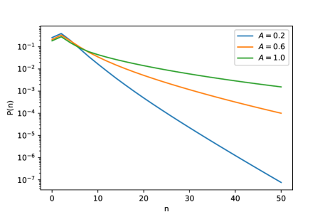
Figure 1: Varying $A$

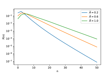
Figure 2: Varying $\widetilde{A}$

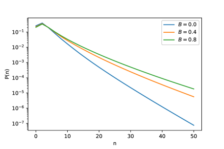
Figure 3: Varying $B$

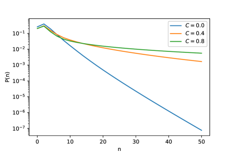
Figure 4: Varying $C$

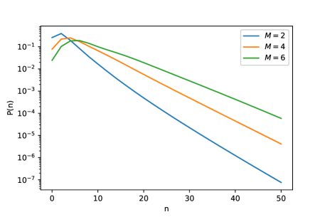
Figure 5: Varying $M$

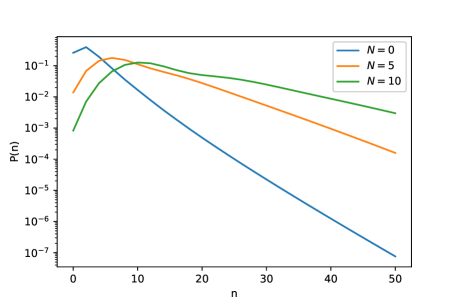
Figure 6: Varying $N$

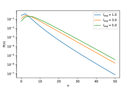
Figure 7: Varying $l_{\text{avg}}$

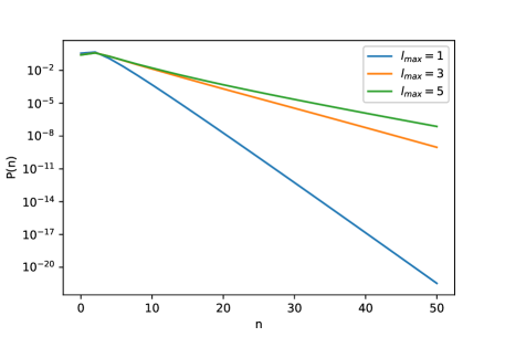
Figure 8: Varying $l_{\text{max}}$

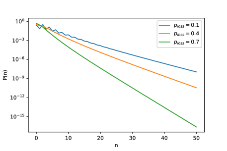
Figure 9: Varying $p_{\text{loss}}$

Higher values of each parameter generally have an effect of broadening the overall distribution. However, some parameters exhibit different behaviour from the rest, and we note several interesting observations below.

Figures 1 and 4 show that high values of $A$ or $C$ produce a noticeable change in gradient at approximately $n=5$. This is very similar to the shoulder-like structure observed in KNO scaling violation, mostly evident in hadronic collisions above $\sqrt{s}=200$ GeV (see Figures 11 to 14). These correspond to gluon branching processes, which suggests they may play an important role in the physics behind KNO scaling violation.

Figures 5 and 6 show that the initial number of quarks ($M$) and gluons ($N$) in the collision affects the position of the distribution’s peak. However, the extremely high values (such as $M=10$ in Figure 6) might introduce oscillations in the final distribution.

Figure 9 shows a potential weakness of the Binomial loss function. At low values (see $p_{\text{loss}}=0.1$ in Figure 9), oscillations occur at multiplicities below $n=20$, reflective of numerical calculation instability. Hence, we would not expect best-fit values of $p_{\text{loss}}$ that are too low.

Together, the nine parameters bring about some effect on the eventual shape of the multiplicity distribution. However, not all effects are independent (e.g. parameters $A$ and $C$); hence, it is certainly plausible that two different sets of parameter values can result in equally good fits to the experimental data. In this work, we limit our scope to demonstrating the ability of the numerical model to describe the data – showing the existence and derivation of comparable solution sets akin to “family of curves” shall be considered in a future work.

4 Fits to experimental data

In this section, we attempt to fit the multiplicity distribution produced by our numerical model against a selection of experimental data: $e^{+}e^{-}$ annihilations at $\sqrt{s}=$ 14, 22, 34.8 and 43.6 GeV from TASSO TASSOCollaboration1989 , $\sqrt{s}=$ 57 GeV from AMY TheAMYCollaboration1990 , $\sqrt{s}=$ 91 GeV from DELPHI Abreu1991 and $\sqrt{s}=$ 133, 161, 172, 183 and 189 GeV from OPAL OPALcollaboration1996 ; OPALcollaboration1997 ; Ackerstaff1997a ; $p\overline{p}$ collisions at $\sqrt{s}=$ 200, 546 and 900 GeV from UA5 Alner1987 ; UA5Collaboration1989 , and $pp$ collisions at $\sqrt{s}=$ 0.9, 2.36 and 7 TeV from CMS Khachatryan2011a . For CMS data, the data point at $n=0$ is omitted.

The best-fit values for the model parameters are searched using a Markov chain Monte Carlo (MCMC) algorithm and are presented in Tables 1-3 for the three types of collisions. Figures 10-14 show semi-log plots of the probability distributions that are measured experimentally (circles with error bars) and generated by our model (solid lines). Finally, to further compare the distributions from data and our model, we give the normalised moments $C_{q}=\langle n^{q}\rangle/\langle n\rangle^{q}$ for $q=$ 2-5 in Tables 4-8.

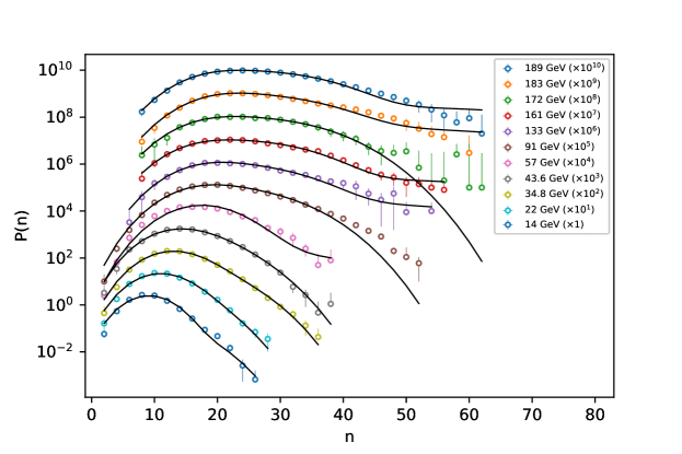
Figure 10: Fits to $e^{+}e^{-}$ collisions (various collaborations)

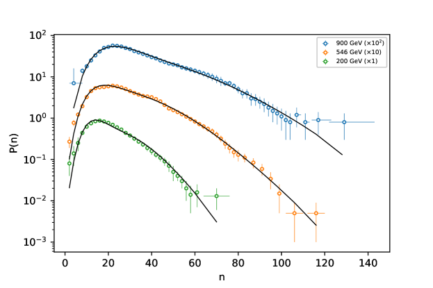
Figure 11: Fits to $\overline{p}p$ collisions (UA5 collaborations)

Figure 12: Fits to $pp$ collisions at $\sqrt{s}=$ 0.9 TeV (CMS collaboration)

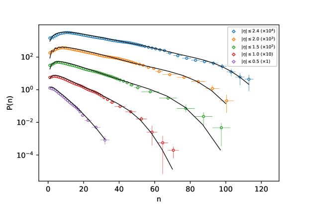
Figure 13: Fits to $pp$ collisions at $\sqrt{s}=$ 2.36 TeV (CMS collaboration)

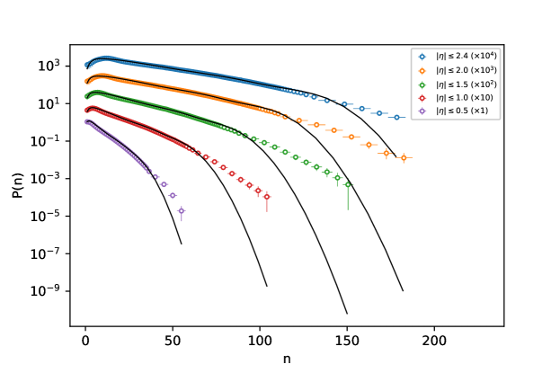
Figure 14: Fits to $pp$ collisions at $\sqrt{s}=$ 7 TeV (CMS collaboration)

Table 1: Best-fit parameters ($e^{+}e^{-}$ collisions, various collaborations)

$\sqrt{s}$ (GeV)	Collab.	$A$	$\widetilde{A}$	$B$	$C$	$M$	$N$	$l_{\text{avg}}$	$l_{\text{max}}$	$\chi^{2}$/d.o.f.
14	TASSO	0.0647	0.0047	0.1164	0.3512	18	0	0.8793	1	16.5642
22	TASSO	0.0135	0.0022	0.1682	0.1659	20	1	0.9492	1	8.6087
34.8	TASSO	0.1370	0.0135	0.3716	0.2929	25	0	0.3910	1	6.9343
43.6	TASSO	0.0175	0.0006	0.4582	0.1048	11	8	0.6484	1	1.0916
57	AMY	0.2833	0.0081	0.0789	0.3993	34	0	0.0173	3	2.7237
91	DELPHI	0.3131	0.0022	0.3513	0.3198	30	2	0.8385	1	5.3986
133	OPAL	0.1143	0.0028	0.2827	0.5884	32	2	0.0666	5	0.5988
161	OPAL	0.4308	0.0008	0.1344	0.4303	31	2	0.0746	4	0.4484
172	OPAL	0.1383	0.0079	0.4149	0.4334	30	3	0.4580	1	0.1392
183	OPAL	0.0340	0.0001	0.1859	0.6935	37	2	0.1220	2	1.4377
189	OPAL	0.0125	0.0097	0.1622	0.7508	34	2	0.1013	2	0.8462

Table 2: Best-fit parameters ($p\overline{p}$ collisions, UA5 collaboration)

$\sqrt{s}$ (GeV)	$A$	$\widetilde{A}$	$B$	$C$	$M$	$N$	$l_{\text{avg}}$	$l_{\text{max}}$	$\chi^{2}$/d.o.f.
200	0.0671	0.1918	0.0842	0.1269	6	6	1.4672	2	0.9352
546	0.2623	0.0607	0.0279	0.1115	0	9	1.9908	2	1.0409
900	0.3073	0.4182	0.6328	0.0591	9	0	1.3253	2	0.3276

Table 3: Best-fit parameters ($pp$ collisions, CMS collaboration)

$\sqrt{s}$ (GeV)	$|\eta|\leq$	$A$	$\widetilde{A}$	$B$	$C$	$M$	$N$	$l_{\text{avg}}$	$l_{\text{max}}$	$p_{\text{loss}}$	$\chi^{2}$/d.o.f.
900	0.5	0.1829	0.2592	0.0134	0.6120	1	2	1.5059	7	0.7306	0.2754
	1.0	0.3430	0.3457	0.0016	0.1073	0	4	1.7684	3	0.5738	0.6614
	1.5	0.1527	0.0944	0.0368	0.2514	1	4	2.0122	3	0.5594	0.3717
	2.0	0.0561	0.3101	0.0089	0.3211	0	5	1.9857	3	0.5586	0.4550
	2.4	0.0348	0.1196	0.0148	0.3448	0	5	2.5459	3	0.5455	0.5009
2360	0.5	0.1893	0.4830	0.0497	0.7593	2	1	1.7598	7	0.7320	0.6909
	1.0	0.0606	0.0419	0.0242	0.2911	0	4	1.8010	3	0.5681	0.6545
	1.5	0.0023	0.0008	0.0534	0.3312	0	4	1.9608	2	0.2805	1.1752
	2.0	0.0124	0.0204	0.0585	0.3523	0	4	1.9992	2	0.1759	1.1930
	2.4	0.1171	0.3178	0.0194	0.3314	0	4	2.8365	3	0.4358	0.4126
7000	0.5	0.0061	0.0002	0.2361	0.3473	0	3	2.0296	3	0.6302	1.5980
	1.0	0.0433	0.0044	0.4275	0.4280	0	4	2.2061	3	0.6200	1.6879
	1.5	0.0477	0.0016	0.2680	0.4598	0	4	2.4886	3	0.6132	1.5041
	2.0	0.0786	0.0062	0.2400	0.4769	0	4	2.6558	3	0.5886	1.1997
	2.4	0.1859	0.0135	0.2934	0.4120	0	4	2.9969	3	0.4793	1.0158

Table 4: Moments for $e^{+}e^{-}$ fits

	$\sqrt{s}=$ 14 GeV			$\sqrt{s}=$ 22 GeV			$\sqrt{s}=$ 34.8 GeV
	Data	Model	% diff.	Data	Model	% diff.	Data	Model	% diff.
$C_{2}$	1.1092	1.1169	0.6887	1.0983	1.1050	0.6067	1.0929	1.0960	0.2890
$C_{3}$	1.3483	1.3608	0.9192	1.3095	1.3239	1.0950	1.2925	1.2994	0.5344
$C_{4}$	1.7833	1.7863	0.1697	1.6813	1.7008	1.1529	1.6429	1.6533	0.6278
$C_{5}$	2.5537	2.5102	1.7181	2.3104	2.3254	0.6500	2.2328	2.2451	0.5488
$\overline{n}$	9.3021	9.2921	0.1074	11.3076	11.3077	0.0010	13.5870	13.5800	0.0515

	$\sqrt{s}=$ 43.6 GeV			$\sqrt{s}=$ 57 GeV			$\sqrt{s}=$ 91 GeV
	Data	Model	% diff.	Data	Model	% diff.	Data	Model	% diff.
$C_{2}$	1.0928	1.0941	0.1153	1.0883	1.0670	1.9758	1.0922	1.0837	0.7812
$C_{3}$	1.2892	1.2917	0.1926	1.2759	1.2065	5.5876	1.2931	1.2602	2.5755
$C_{4}$	1.6272	1.6304	0.1997	1.5984	1.4402	10.4107	1.6483	1.5598	5.5141
$C_{5}$	2.1818	2.1849	0.1405	2.1251	1.8108	15.9699	2.2469	2.0402	9.6455
$\overline{n}$	15.0775	15.0877	0.0675	17.4905	17.9617	2.6578	21.1974	21.2994	0.4798

	$\sqrt{s}=$ 133 GeV			$\sqrt{s}=$ 161 GeV			$\sqrt{s}=$ 172 GeV
	Data	Model	% diff.	Data	Model	% diff.	Data	Model	% diff.
$C_{2}$	1.1045	1.0957	0.7944	1.0976	1.0972	0.0302	1.0899	1.0829	0.6467
$C_{3}$	1.3376	1.3087	2.1856	1.3116	1.3122	0.0456	1.2868	1.2563	2.3976
$C_{4}$	1.7613	1.6971	3.7112	1.6932	1.7018	0.5085	1.6381	1.5471	5.7105
$C_{5}$	2.4973	2.3808	4.7791	2.3445	2.3842	1.6773	2.2399	2.0059	11.0190
$\overline{n}$	23.6105	23.2516	1.5318	24.4486	24.4297	0.0775	25.5395	25.1615	1.4913

	$\sqrt{s}=$ 183 GeV			$\sqrt{s}=$ 189 GeV
	Data	Model	% diff.	Data	Model	% diff.
$C_{2}$	1.0970	1.1008	0.3502	1.0977	1.1004	0.2446
$C_{3}$	1.3118	1.3324	1.5591	1.3118	1.3265	1.1095
$C_{4}$	1.6959	1.7705	4.3081	1.6933	1.7462	3.0756
$C_{5}$	2.3475	2.5737	9.1907	2.3423	2.5018	6.5839
$\overline{n}$	26.8559	26.8359	0.0747	26.9417	26.7879	0.5723

Table 5: Moments for $p\overline{p}$ fits

	$\sqrt{s}=$ 200 GeV			$\sqrt{s}=$ 546 GeV			$\sqrt{s}=$ 900 GeV
	Data	Model	% diff.	Data	Model	% diff.	Data	Model	% diff.
$C_{2}$	1.2554	1.2562	0.0674	1.2745	1.2763	0.1449	1.3005	1.2862	1.0991
$C_{3}$	1.8813	1.8828	0.0799	1.9522	1.9634	0.5708	2.0807	2.0230	2.8112
$C_{4}$	3.2437	3.2200	0.7350	3.4410	3.4765	1.0279	3.8946	3.6999	5.1265
$C_{5}$	6.2519	6.0740	2.8865	6.7616	6.8537	1.3524	8.2073	7.5568	8.2527
$\overline{n}$	21.3541	21.5906	1.1013	29.1962	29.1271	0.2369	35.6190	35.6841	0.1826

Table 6: Moments for $pp$ fits ($\sqrt{s}=$ 0.9 TeV)

	$|\eta|<0.5$			$|\eta|<1.0$			$|\eta|<1.5$
	Data	Model	% diff.	Data	Model	% diff.	Data	Model	% diff.
$C_{2}$	1.5815	1.5808	0.0474	1.5703	1.5429	1.7599	1.5385	1.5256	0.8377
$C_{3}$	3.3862	3.3965	0.3050	3.2723	3.1682	3.2346	3.0920	3.0439	1.5690
$C_{4}$	8.8935	8.9659	0.8117	8.2287	7.8883	4.2249	7.4131	7.2363	2.4142
$C_{5}$	27.0125	27.3465	1.2289	23.6416	22.4624	5.1156	20.1156	19.3766	3.7425
$\overline{n}$	4.4260	4.4210	0.1138	8.0591	8.1412	1.0142	11.7442	11.7857	0.3527

	$|\eta|<2.0$			$|\eta|<2.4$
	Data	Model	% diff.	Data	Model	% diff.
$C_{2}$	1.5040	1.5011	0.1958	1.4738	1.4739	0.0043
$C_{3}$	2.9123	2.9093	0.1006	2.7593	2.7587	0.0192
$C_{4}$	6.6587	6.6529	0.0869	6.0415	6.0207	0.3456
$C_{5}$	17.0947	17.0034	0.5355	14.7476	14.5723	1.1959
$\overline{n}$	15.5073	15.4859	0.1381	18.4315	18.4310	0.0030

Table 7: Moments for $pp$ fits ($\sqrt{s}=$ 2.36 TeV)

	$|\eta|<0.5$			$|\eta|<1.0$			$|\eta|<1.5$
	Data	Model	% diff.	Data	Model	% diff.	Data	Model	% diff.
$C_{2}$	1.5848	1.5734	0.7274	1.5657	1.5429	1.4687	1.5229	1.4877	2.3379
$C_{3}$	3.3344	3.2780	1.7072	3.1870	3.1040	2.6408	2.9579	2.8375	4.1537
$C_{4}$	8.4428	8.1971	2.9526	7.7060	7.4336	3.5992	6.7493	6.4189	5.0191
$C_{5}$	24.4903	23.4034	4.5389	21.2185	20.2147	4.8457	17.4755	16.5657	5.3451
$\overline{n}$	5.2887	5.2907	0.0391	9.7229	9.7775	0.5601	13.9685	14.0468	0.5584

	$|\eta|<2.0$			$|\eta|<2.4$
	Data	Model	% diff.	Data	Model	% diff.
$C_{2}$	1.4902	1.4656	1.6702	1.4707	1.4685	0.1519
$C_{3}$	2.8084	2.7311	2.7933	2.7363	2.7418	0.1983
$C_{4}$	6.1951	6.0161	2.9321	6.0084	6.0757	1.1138
$C_{5}$	15.4530	15.0953	2.3415	15.0915	15.4570	2.3926
$\overline{n}$	18.3244	18.2059	0.6491	21.6960	21.4683	1.0553

Table 8: Moments for $pp$ fits ($\sqrt{s}=$ 7 TeV)

	$|\eta|<0.5$			$|\eta|<1.0$			$|\eta|<1.5$
	Data	Model	% diff.	Data	Model	% diff.	Data	Model	% diff.
$C_{2}$	1.7322	1.7097	1.3103	1.7054	1.6818	1.3928	1.6689	1.6536	0.9216
$C_{3}$	4.1591	4.0604	2.4030	3.9448	3.8424	2.6298	3.7259	3.6570	1.8662
$C_{4}$	12.2449	11.8190	3.5396	11.0204	10.5832	4.0474	9.9568	9.6605	3.0209
$C_{5}$	41.4444	39.3070	5.2939	35.0436	32.9025	6.3022	30.1089	28.6587	4.9354
$\overline{n}$	6.9240	6.9915	0.9700	13.1220	13.2729	1.1435	19.4220	19.5972	0.8985

	$|\eta|<2.0$			$|\eta|<2.4$
	Data	Model	% diff.	Data	Model	% diff.
$C_{2}$	1.6402	1.6331	0.4338	1.6161	1.6074	0.5374
$C_{3}$	3.5647	3.5333	0.8849	3.4326	3.3998	0.9610
$C_{4}$	9.2037	9.0740	1.4192	8.6134	8.5062	1.2522
$C_{5}$	26.6864	26.0505	2.4116	24.1689	23.7581	1.7145
$\overline{n}$	25.8712	26.0038	0.5111	30.7905	30.9391	0.4815

5 Discussion

5.1 $e^{+}e^{-}$ annihilations

It is immediately apparent that with values of $\chi^{2}$/d.o.f. $\gg 1$ in most of our fits below $\sqrt{s}=$ 133 GeV, our model does not exactly describe $e^{+}e^{-}$ annihilation well. Considering that the initial interaction is leptonic rather than hadronic, a complete description would certainly require elements outside QCD (e.g. QED) to be built in. Furthermore, $e^{+}e^{-}$ annihilations can result in a variety of final states, and the only one that leads to a scenario described by our model is $e^{+}e^{-}\rightarrow\gamma\rightarrow q\overline{q}$ (electron-position annihilation followed by quark-antiquark pair production). Our model does not account for the other possible interactions.

Considering how the GMD fits excellently to the same set of $e^{+}e^{-}$ data Dewanto2008 , our model is evidently not a direct extension of the GMD, even though the latter is a partial solution to Giovannini’s parton branching equation. However, the fitting results do have an interesting connection – in the GMD, the fitting parameters $k$ and $k^{\prime}$ are interpreted as the average initial number of quarks and gluons respectively in the branching process Chan1990 . These are $M$ and $N$ respectively in our formulation, and we can see that unlike hadronic collisions, the branching cascade that results from $e^{+}e^{-}$ annihilation typically begins with many ($>10$) partons, in agreement with [29].

5.2 $p\overline{p}$ collisions

From Table 2, the highest $\chi^{2}$/d.o.f. value obtained is 1.0185, which suggests that our model describes the observed data fairly well. The normalised moments from Table 5 also suggest good agreement between data and model, except for the fit at $\sqrt{s}=$ 900 GeV, where the model fails to capture the tail of the distribution.

5.3 $pp$ collisions

From Table 3, apart from the fit at $\sqrt{s}=$ 7 TeV and $|\eta|<1.0$, the $\chi^{2}$/d.o.f. values are generally much smaller than unity. This suggests that our model describes $pp$ collisions at the TeV scale fairly well. Furthermore, the normalised moments agree with each other to within 7.08%, with the majority within 1%. However, upon visual inspection, our model does not produce the shoulder-like structure characteristic of KNO scaling violation.

Furthermore, the tails of the produced distributions fall off towards zero faster than the data points. One possible explanation could be that the data points at higher-multiplicity bins are aggregated together in the CMS data, which affected the ability of our optimisation algorithm to reproduce the distribution shape in better detail.

5.4 The binomial loss function

From Table 3, a clear trend for fitted values of the loss parameter $p_{\text{loss}}$ can be observed for $\sqrt{s}=$ 900 GeV and 7 TeV. $p_{\text{loss}}$ increased as the pseudorapidity interval decreased, in agreement with the physical notion behind stage 4 of our model. However, the trend did not show for $\sqrt{s}=$ 2.36 TeV, suggesting that the model is not sufficiently robust.

It must also be noted that the set of values for $p_{\text{loss}}$ for $\sqrt{s}=$ 900 GeV and 7 TeV do not agree with each other exactly, even though the trend within each energy makes sense. This implies that the binomial loss function does not just account for the reduced pseudorapidity space, but gets influenced by other factors as well. Still, it works as a rough approximation to describing data from reduced pseudorapidity space. In future work, the binomial loss function could be improved to become more sophisticated and realistic.

5.5 Increase in gluonic activity at the TeV scale

Chan and Chew remarked that gluon branching would become increasingly dominant as the centre-of-mass energy $\sqrt{s}$ increases into the TeV regime Chan1990 . In the context of the GMD, this would manifest itself via the parameters $k$ approaching zero and $k^{\prime}$ increasing above 3.0, which turns the GMD into the Furry-Yule distribution (FYD, which is another special case of the GMD where $k=0$). We observe these predictions validated in our results – from Table 3, the fitted values of $\widetilde{A}$ decreases as $\sqrt{s}$ increases from 0.9 to 7 TeV, which is characteristic of a Furry-Yule process. Also, the fraction of initial partons being gluons also increases, and the values of $C$ (probability of $g\rightarrow ggg$) increases. Together, our data strongly agrees with their prediction.

It must be noted that the best-fit parameters presented in section 4 are by no means representative of the absolute global minimum values for $\chi^{2}$. The parameter space is infinitely dense to be sampled thoroughly; instead, they are the best-possible result found using an optimisation heuristic within available computational resources. Since $\chi^{2}$ in our model is a function of 8 to 9 parameters, it is entirely conceivable that distinct parameter sets could result in very comparable $\chi^{2}$ values. In particular, the multiplicity distributions published by experiments are a result of averaging over numerous events, and are certainly not describable by a fixed integer value of $M$ and $N$.

6 Prediction for $\sqrt{s}=$ 14 TeV

Based on the best-fit values summarised in Table 3, we attempt to make a prediction for $pp$ collisions at $\sqrt{s}=$ 14 TeV. We continue to expect gluonic activity to be dominant, which would manifest itself in the following ways:

1. Processes $A$, $B$ and $C$ would become even more prominent, and hence their values would increase.

2. Process $\widetilde{A}$ would decrease further towards zero.

3. Each parton would hadronise into more hadrons, and hence $l_{\text{avg}}$ and $l_{\text{max}}$ would increase above 3.

4. The initial conditions would still be best described by the presence of only gluons and no quarks.

5. The overall probability of gluon branching $A+B+C$ appears to increase with $\sqrt{s}$. However, at $\sqrt{s}=$ 7 TeV, $A+B+C=0.8913$ which is nearing the upper bound of 1 (conservation of probability). Hence, the value of $T$ would need to increase beyond 3.0 for the model to describe the final multiplicity distribution for $\sqrt{s}=$ 14 TeV (see comments in section 2, stage 1).

7 Conclusion

A numerical model for producing charged-particle multiplicity distributions has been presented. It has been shown to describe hadronic collision data well up to the TeV scale, but less so for lower-energy leptonic interactions. This work has also shown that within the framework of pQCD and multiparticle production, Giovannini’s parton branching equations remain valid up to the TeV scales currently being explored at the LHC. Our model suggests that the increase in gluonic activity as $\sqrt{s}$ increases in hadronic collisions can be attributed to a higher proportion to gluon branching and initial gluon number, in agreement with earlier predictions by Chan and Chew Chan1990 .

- (1) A.H. Chan, C.K. Chew, Phys. Rev. D 41(3), 851 (1990). DOI 10.1103/PhysRevD.41.851
- (2) UA5 Collaboration, Phys. Lett. B 167(4), 476 (1986). DOI 10.1016/0370-2693(86)91304-3
- (3) P. Ghosh, Phys. Rev. D - Part. Fields, Gravit. Cosmol. 85(5), 1 (2012). DOI 10.1103/PhysRevD.85.054017
- (4) I. Zborovský, Eur. Phys. J. C 78(10), 816 (2018). DOI 10.1140/epjc/s10052-018-6287-x. URL http://link.springer.com/10.1140/epjc/s10052-018-6287-x
- (5) A. Giovannini, Nucl. Physics, Sect. B 161(2-3), 429 (1979). DOI 10.1016/0550-3213(79)90222-0
- (6) M. Biyajima, Prog. Theor. Phys. 69(3), 966 (1983). DOI 10.1143/PTP.69.966. URL https://academic.oup.com/ptp/article-lookup/doi/10.1143/PTP.69.966
- (7) M. Biyajima, Phys. Lett. B 137(3-4), 225 (1984). DOI 10.1016/0370-2693(84)90234-X
- (8) M. Biyajima, Phys. Lett. B 139(1-2), 93 (1984). DOI 10.1016/0370-2693(84)90042-X
- (9) M. Biyajima, N. Suzuki, Phys. Lett. B 143(4-6), 463 (1984). DOI 10.1016/0370-2693(84)91503-X
- (10) M. Biyajima, K. Shirane, N. Suzuki, Phys. Rev. D 37(7), 1824 (1988). DOI 10.1103/PhysRevD.37.1824. URL https://link.aps.org/doi/10.1103/PhysRevD.37.1824
- (11) N. Suzuki, M. Biyajima, G. Wilk, Phys. Lett. B 268(3-4), 447 (1991). DOI 10.1016/0370-2693(91)91606-V
- (12) C.C. Shih, Phys. Rev. D 33(11), 3391 (1986). DOI 10.1103/PhysRevD.33.3391
- (13) P. Carruthers, C. Shih, Int. J. Mod. Phys. A 02(05), 1447 (1987). DOI 10.1142/S0217751X87000806. URL https://www.worldscientific.com/doi/abs/10.1142/S0217751X87000806
- (14) B. Durand, I. Sarcevic, Phys. Lett. B 172(1), 104 (1986). DOI 10.1016/0370-2693(86)90225-X. URL https://linkinghub.elsevier.com/retrieve/pii/037026938690225X
- (15) B. Durand, I. Sarcevic, Phys. Rev. D 36(9), 2693 (1987). DOI 10.1103/PhysRevD.36.2693
- (16) S. Sakai, Phys. Rev. D 40(5), 1430 (1989). DOI 10.1103/PhysRevD.40.1430
- (17) V. Gupta, N. Sarma, Zeitschrift für Phys. C Part. Fields 52(1), 53 (1991). DOI 10.1007/BF01412326. URL http://link.springer.com/10.1007/BF01412326
- (18) R.C. Hwa, Zeitschrift für Phys. C Part. Fields 38(1), 277 (1988). DOI 10.1007/BF01574550
- (19) A.H. Chan, C.K. Chew, J. Math. Phys. 33(9), 3209 (1992). DOI 10.1063/1.529539
- (20) The CMS Collaboration, J. High Energy Phys. 2011(1) (2011). DOI 10.1007/JHEP01(2011)079
- (21) TASSO Collaboration, Zeitschrift für Phys. C Part. Fields 45(2), 193 (1989). DOI 10.1007/BF01674450. URL http://link.springer.com/10.1007/BF01674450
- (22) The AMY Collaboration, Phys. Rev. D 42(3), 737 (1990). DOI 10.1103/PhysRevD.42.737. URL https://link.aps.org/doi/10.1103/PhysRevD.42.737
- (23) DELPHI Collaboration, Zeitschrift für Phys. C Part. Fields 50(2), 185 (1991). DOI 10.1007/BF01474073. URL http://link.springer.com/10.1007/BF01474073
- (24) OPAL Collaboration, Zeitschrift für Phys. C Part. Fields 72(2), 191 (1996). DOI 10.1007/s002880050237. URL http://link.springer.com/10.1007/s002880050237
- (25) OPAL Collaboration, Zeitschrift fur Phys. C-Particles Fields 75(2), 193 (1997). DOI 10.1007/s002880050462. URL http://link.springer.com/10.1007/s002880050462
- (26) The OPAL Collaboration, Eur. Phys. J. C 16(2), 185 (2000). DOI 10.1007/s100520050015. URL http://link.springer.com/10.1007/s100520050015
- (27) UA5 Collaboration, Phys. Rep. 154(5-6), 247 (1987). DOI 10.1016/0370-1573(87)90130-X. URL http://www.sciencedirect.com/science/article/pii/037015738790130Xhttps://linkinghub.elsevier.com/retrieve/pii/037015738790130X
- (28) UA5 Collaboration, Zeitschrift für Phys. C Part. Fields 43(3), 357 (1989). DOI 10.1007/BF01506531
- (29) A. Dewanto, A.H. Chan, C.H. Oh, R. Chen, K. Sitaram, Eur. Phys. J. C 57(3), 515 (2008). DOI 10.1140/epjc/s10052-008-0750-z