DPMC: Weighted Model Counting by Dynamic Programming on Project-Join Trees

Abstract

We propose a unifying dynamic-programming framework to compute exact literal-weighted model counts of formulas in conjunctive normal form. At the center of our framework are project-join trees, which specify efficient project-join orders to apply additive projections (variable eliminations) and joins (clause multiplications). In this framework, model counting is performed in two phases. First, the planning phase constructs a project-join tree from a formula. Second, the execution phase computes the model count of the formula, employing dynamic programming as guided by the project-join tree. We empirically evaluate various methods for the planning phase and compare constraint-satisfaction heuristics with tree-decomposition tools. We also investigate the performance of different data structures for the execution phase and compare algebraic decision diagrams with tensors. We show that our dynamic-programming model-counting framework DPMC is competitive with the state-of-the-art exact weighted model counters Cachet, c2d, d4, and miniC2D.

1 Introduction

Model counting is a fundamental problem in artificial intelligence, with applications in machine learning, probabilistic reasoning, and verification [24, 34, 50]. Given an input set of constraints, with the focus in this paper on Boolean constraints, the model-counting problem is to count the number of satisfying assignments. Although this problem is #P-Complete [69], a variety of tools exist that can handle industrial sets of constraints, e.g., [58, 52, 19, 46].

Dynamic programming is a powerful technique that has been applied across computer science [7], including to model counting [4, 56, 36]. The key idea is to solve a large problem by solving a sequence of smaller subproblems and then incrementally combining these solutions into the final result. Dynamic programming provides a natural framework to solve a variety of problems defined on sets of constraints: subproblems can be formed by partitioning the constraints. This framework has been instantiated into algorithms for database-query optimization [48], satisfiability solving [68, 2, 54], and QBF evaluation [11].

Dynamic programming has also been the basis of several tools for model counting [26, 25, 27, 31]. Although each tool uses a different data structure–algebraic decision diagrams (ADDs) [26], tensors [25, 27], or database tables [31]–the overall algorithms have similar structure. The goal of this work is to unify these approaches into a single conceptual framework: project-join trees. Project-join trees are not an entirely new idea. Similar concepts have been used in constraint programming (as join trees [22]), probabilistic inference (as cluster trees [60]), and database-query optimization (as join-expression trees [48]). Our original contributions include the unification of these concepts into project-join trees and the application of this unifying framework to model counting.

We argue that project-join trees provide the natural formalism to describe execution plans for dynamic-programming algorithms for model counting. In particular, considering project-join trees as execution plans enables us to decompose dynamic-programming algorithms such as the one in [26] into two phases, following the breakdown in [27]: a planning phase and an execution phase. This enables us to study and compare different planning algorithms, different execution environments, and the interplay between planning and execution. Such a study is the main focus of this work. While the focus here is on model counting, our framework is of broader interest. For example, in [65], Tabajara and Vardi described a dynamic-programming, binary-decision-diagram-based framework for functional Boolean synthesis. Refactoring the algorithm into a planning phase followed by an execution phase is also of interest in that context.

The primary contribution of the work here is a dynamic-programming framework for weighted model counting based on project-join trees. In particular:

1. We show that several recent algorithms for weighted model counting [26, 25, 31] can be unified into a single framework using project-join trees.

2. We compare the one-shot constraint-satisfaction heuristics used in [26] with the anytime tree-decomposition tools used in [25] and observe that tree-decomposition tools outperform constraint-satisfaction heuristics.

3. We compare (sparse) ADDs [5] with (dense) tensors [38] and find that ADDs outperform tensors on single CPU cores.

4. We find that project-join-tree-based algorithms contribute to a portfolio of model counters containing Cachet [58], c2d [19], d4 [46], and miniC2D [52].

These conclusions have significance beyond model counting. The superiority of anytime tree-decomposition tools over classical one-shot constraint-satisfaction heuristics can have broad applicability. Similarly, the advantage of compact data structures for dynamic programming may apply to other optimization problems.

2 Preliminaries

Pseudo-Boolean Functions and Early Projection

A pseudo-Boolean function over a set $X$ of variables is a function $f:2^{X}\to\mathbb{R}$. Operations on pseudo-Boolean functions include product and projection. First, we define product.

Definition 1 (Product)

Let $X$ and $Y$ be sets of Boolean variables. The product of functions $f:2^{X}\to\mathbb{R}$ and $g:2^{Y}\to\mathbb{R}$ is the function $f\cdot g:2^{X\cup Y}\to\mathbb{R}$ defined for all $\tau\in 2^{X\cup Y}$ by $(f\cdot g)(\tau)\equiv f(\tau\cap X)\cdot g(\tau\cap Y).$

Next, we define (additive) projection, which marginalizes a single variable.

Definition 2 (Projection)

Let $X$ be a set of Boolean variables and $x\in X$. The projection of a function $f:2^{X}\to\mathbb{R}$ w.r.t. $x$ is the function $\sum_{x}f:2^{X\setminus\left\{x\right\}}\to\mathbb{R}$ defined for all $\tau\in 2^{X\setminus\left\{x\right\}}$ by $\left(\sum_{x}f\right)(\tau)\equiv f(\tau)+f(\tau\cup\left\{x\right\}).$

Note that projection is commutative, i.e., that $\sum_{x}\sum_{y}f=\sum_{y}\sum_{x}f$ for all variables $x,y\in X$ and functions $f:2^{X}\to\mathbb{R}$. Given a set $X=\left\{x_{1},x_{2},\ldots,x_{n}\right\}$, define $\sum_{X}f\equiv\sum_{x_{1}}\sum_{x_{2}}\ldots\sum_{x_{n}}f$. Our convention is that $\sum_{\varnothing}f\equiv f$.

When performing a product followed by a projection, it is sometimes possible to perform the projection first. This is known as early projection [48].

Theorem 2.1 (Early Projection)

Let $X$ and $Y$ be sets of variables. For all functions $f:2^{X}\to\mathbb{R}$ and $g:2^{Y}\to\mathbb{R}$, if $x\in X\setminus Y$, then $\sum_{x}(f\cdot g)=\left(\sum_{x}f\right)\cdot g.$

Early projection is a key technique in symbolic computation in a variety of settings, including database-query optimization [40], symbolic model checking [9], satisfiability solving [54], and model counting [26].

Weighted Model Counting

We compute the total weight, subject to a given weight function, of all models of an input propositional formula. Formally:

Definition 3 (Weighted Model Count)

Let $X$ be a set of Boolean variables, $\varphi:2^{X}\to\{0,1\}$ be a Boolean function, and $W:2^{X}\to\mathbb{R}$ be a pseudo-Boolean function. The weighted model count of $\varphi$ w.r.t. $W$ is $W(\varphi)\equiv\sum_{\tau\in 2^{X}}\varphi(\tau)\cdot W(\tau)$.

The weighted model count of $\varphi$ w.r.t. $W$ can be naturally expressed in terms of pseudo-Boolean functions: $W(\varphi)=\left(\sum_{X}(\varphi\cdot W)\right)(\varnothing)$. The function $W:2^{X}\to\mathbb{R}$ is called a weight function. In this work, we focus on literal-weight functions, which can be expressed as products of weights associated with each variable. Formally, a literal-weight function $W$ can be factored as $W=\prod_{x\in X}W_{x}$ for pseudo-Boolean functions $W_{x}:2^{\{x\}}\to\mathbb{R}$.

Graphs

A graph $G$ has a set $\mathcal{V}(G)$ of vertices, a set $\mathcal{E}(G)$ of (undirected) edges, a function $\delta_{G}:\mathcal{V}(G)\to 2^{\mathcal{E}(G)}$ that gives the set of edges incident to each vertex, and a function $\epsilon_{G}:\mathcal{E}(G)\to 2^{\mathcal{V}(G)}$ that gives the set of vertices incident to each edge. Each edge must be incident to exactly two vertices, but multiple edges can exist between two vertices. A tree is a simple, connected, and acyclic graph. A leaf of a tree $T$ is a vertex of degree one, and we use $\mathcal{L}(T)$ to denote the set of leaves of $T$. We often refer to a vertex of a tree as a node and an edge as an arc to avoid confusion. A rooted tree is a tree $T$ together with a distinguished node $r\in\mathcal{V}(T)$ called the root. In a rooted tree $(T,r)$, each node $n\in\mathcal{V}(T)$ has a (possibly empty) set of children, denoted $\mathcal{C}(n)$, which contains all nodes $n^{\prime}$ adjacent to $n$ s.t. all paths from $n^{\prime}$ to $r$ contain $n$.

3 Using Project-Join Trees for Weighted Model Counting

In model counting, a Boolean formula is often given in conjunctive normal form (CNF), i.e., as a set $\varphi$ of clauses. For each clause $c\in\varphi$, define $\texttt{Vars}(c)$ to be the set of variables appearing in $c$. Then $c$ represents a Boolean function over $\texttt{Vars}(c)$. Similarly, $\varphi$ represents a Boolean function over $\texttt{Vars}(\varphi)\equiv\bigcup_{c\in\varphi}\texttt{Vars}(c)$.

It is well-known that weighted model counting can be performed through a sequence of projections and joins on pseudo-Boolean functions [26, 25]. Given a CNF formula $\varphi$ and a literal-weight function $W$ over a set $X$ of variables, the corresponding weighted model count can be computed as follows:

$$W(\varphi)=\left(\sum_{X}\left(\prod_{c\in\varphi}c\cdot\prod_{x\in X}W_{x}\right)\right)(\varnothing)$$ (1)

By taking advantage of the associative and commutative properties of multiplication as well as the commutative property of projection, we can rearrange Equation (1) to apply early projection. It was shown in [26] that early projection can significantly reduce computational cost. There are a variety of possible rearrangements of Equation (1) of varying costs. Although [26] considered several heuristics for performing this rearrangement (using bucket elimination [20] and Bouquet’s Method [8]), they did not attempt to analyze rearrangements.

In this work, we aim to analyze the quality of the rearrangement, in isolation from the underlying implementation and data structure used for Equation (1). This approach has been highly successful for database-query optimization [48], where the central object of theoretical reasoning is the query plan. The approach has also seen similar success in Bayesian network inference [18].

We model a rearrangement of Equation (1) as a project-join tree:

Definition 4 (Project-Join Tree)

Let $X$ be a set of Boolean variables and $\varphi$ be a CNF formula over $X$. A project-join tree of $\varphi$ is a tuple $(T,r,\gamma,\pi)$ where:

• $T$ is a tree with root $r\in\mathcal{V}(T)$,

• $\gamma:\mathcal{L}(T)\to\varphi$ is a bijection between the leaves of $T$ and the clauses of $\varphi$, and

• $\pi:\mathcal{V}(T)\setminus\mathcal{L}(T)\to 2^{X}$ is a labeling function on internal nodes.

Moreover, $(T,r,\gamma,\pi)$ must satisfy the following two properties:

1. $\{\pi(n):n\in\mathcal{V}(T)\setminus\mathcal{L}(T)\}$ is a partition of $X$, and

2. for each internal node $n\in\mathcal{V}(T)\setminus\mathcal{L}(T)$, variable $x\in\pi(n)$, and clause $c\in\varphi$ s.t. $x$ appears in $c$, the leaf node $\gamma^{-1}(c)$ must be a descendant of $n$ in $T$.

If $n$ is a leaf node, then $n$ corresponds to a clause $c=\gamma(n)$ in Equation (1). If $n$ is an internal node, then $n$’s children $\mathcal{C}(n)$ are to be multiplied before the projections of variables in $\pi(n)$ are performed. The two properties ensure that the resulting expression is equivalent to Equation (1) using early projection. See Figure 1 for a graphical example of a project-join tree.

Figure 1: A project-join tree $(T,n_{8},\gamma,\pi)$ of a CNF formula $\varphi$. Each leaf node is labeled by $\gamma$ with a clause of $\varphi$. Each internal node is labeled by $\pi$ with a set of variables of $\varphi$.

Project-join trees have previously been studied in the context of database-query optimization [48]. Project-join trees are closely related to contraction trees in the context of tensor networks [28, 25]. Once a rearrangement of Equation (1) has been represented by a project-join tree, we can model the computation process according to the rearrangement. In particular, given a literal-weight function $W=\prod_{x\in X}W_{x}$, we define the $W$-valuation of each node $n\in\mathcal{V}(T)$ as a pseudo-Boolean function associated with $n$. The $W$-valuation of a node $n\in\mathcal{V}(T)$ is denoted $f^{W}_{n}$ and defined as follows:

$$f^{W}_{n}\equiv\begin{cases}\gamma(n)&\text{if}~{}n\in\mathcal{L}(T)\\ \sum_{\pi(n)}\left(\prod_{o\in\mathcal{C}(n)}f^{W}_{o}\cdot\prod_{x\in\pi(n)}W_{x}\right)&\text{if}~{}n\notin\mathcal{L}(T)\end{cases}$$ (2)

Note that the $W$-valuation of a leaf node $n\in\mathcal{L}(T)$ is a clause $c=\gamma(n)\in\varphi$, interpreted in this context as an associated function $\lambda_{c}:2^{\texttt{Vars}(c)}\to\left\{0,1\right\}$ where $\lambda_{c}(\tau)=1$ if and only if the truth assignment $\tau$ satisfies $c$. The main idea is that the $W$-valuation at each node of $T$ is a pseudo-Boolean function computed as a subexpression of Equation (1). The $W$-valuation of the root is exactly the result of Equation (1), i.e., the weighted model count of $\varphi$ w.r.t. $W$:

Theorem 3.1

Let $\varphi$ be a CNF formula over a set $X$ of variables, $(T,r,\gamma,\pi)$ be a project-join tree of $\varphi$, and $W$ be a literal-weight function over $X$. Then $f^{W}_{r}(\varnothing)=W(\varphi)$.

This gives us a two-phase algorithm for computing the weighted model count of a formula $\varphi$. First, in the planning phase, we construct a project-join tree $(T,r,\gamma,\pi)$ of $\varphi$. We discuss algorithms for constructing project-join trees in Section 4. Second, in the execution phase, we compute $f^{W}_{r}$ by following Equation (2). We discuss data structures for computing Equation (2) in Section 5.

When computing a $W$-valuation, the number of variables that appear in each intermediate pseudo-Boolean function has a significant impact on the runtime. The set of variables that appear in the $W$-valuation of a node is actually independent of $W$. In particular, for each node $n\in\mathcal{V}(T)$, define $\texttt{Vars}(n)$ as follows:

$$\texttt{Vars}(n)\equiv\begin{cases}\texttt{Vars}(\gamma(n))&\text{if}~{}n\in\mathcal{L}(T)\\ \left(\bigcup_{o\in\mathcal{C}(n)}\texttt{Vars}(o)\right)\setminus\pi(n)&\text{if}~{}n\notin\mathcal{L}(T)\end{cases}$$ (3)

For every literal-weight function $W$, the domain of the function $f^{W}_{n}$ is $2^{\texttt{Vars}(n)}$. To characterize the difficulty of $W$-valuation, we define the size of a node $n$, $\texttt{size}(n)$, to be $\left|\texttt{Vars}(n)\right|$ for leaf nodes and $\left|\texttt{Vars}(n)\cup\pi(n)\right|$ for internal nodes. The width of a project-join tree $(T,r,\gamma,\pi)$ is $\texttt{width}(T)\equiv\max_{n\in\mathcal{V}(T)}\texttt{size}(n)$. We see in Section 6 how the width impacts the computation of $W$-valuations.

4 Planning Phase: Building a Project-Join Tree

In the planning phase, we are given a CNF formula $\varphi$ over Boolean variables $X$. The goal is to construct a project-join tree of $\varphi$. In this section, we present two classes of techniques that have been applied to model counting: using constraint-satisfaction heuristics (in [26]) and using tree decompositions (in [25, 31]).

4.1 Planning with One-Shot Constraint-Satisfaction Heuristics

A variety of constraint-satisfaction heuristics for model counting were presented in a single algorithmic framework by [26]. These heuristics have a long history in constraint programming [21], database-query optimization [48], and propositional reasoning [54]. In this section, we adapt the framework of [26] to produce project-join trees. This algorithm is presented as Algorithm 1, which constructs a project-join tree of a CNF formula using constraint-satisfaction heuristics. The functions ClusterVarOrder, ClauseRank, and ChosenCluster represent heuristics for fine-tuning the specifics of the algorithm. Before discussing the various heuristics, we assert the correctness of Algorithm 1 in the following theorem.

Theorem 4.1

Let $X$ be a set of variables and $\varphi$ be a CNF formula over $X$. Assume that ClusterVarOrder returns an injection $X\to\mathbb{N}$. Furthermore, assume that all ClauseRank and ChosenCluster calls satisfy the following conditions:

1. $1\leq\texttt{ClauseRank}(c,\rho)\leq m$,

2. $i<\texttt{ChosenCluster}(n_{i})\leq m$, and

3. $X_{s}\cap\texttt{Vars}(n_{i})=\varnothing$ for all integers $s$ where $i<s<\texttt{ChosenCluster}(n_{i})$.

Then Algorithm 1 returns a project-join tree of $\varphi$.

Input: $X$: set of $m\geq 1$ Boolean variables

Input: $\varphi$: CNF formula over $X$

Output: $(T,r,\gamma,\pi)$: project-join tree of $\varphi$

1 $(T,\texttt{null},\gamma,\pi)\leftarrow\text{empty project-join tree}$

$\rho\leftarrow\texttt{ClusterVarOrder}(\varphi)$

  /* injection $\rho:X\to\mathbb{N}$ */

2 for $i=m,m-1,\ldots,1$ 

       $\Gamma_{i}\leftarrow\left\{c\in\varphi:\texttt{ClauseRank}(c,\rho)=i\right\}$

        /* $1\leq\texttt{ClauseRank}(c,\rho)\leq m$ */

3       $\kappa_{i}\leftarrow\left\{\texttt{LeafNode}(T,c):c\in\Gamma_{i}\right\}$

      

        /* for each $c$, a leaf $l$ with $\gamma(l)=c$ is constructed and put in cluster $\kappa_{i}$ */

       $X_{i}\leftarrow\texttt{Vars}(\Gamma_{i})\setminus\bigcup_{j=i+1}^{m}\texttt{Vars}(\Gamma_{j})$

        /* $\left\{X_{i}\right\}_{i=1}^{m}$ is a partition of $X$ */

4      

5

6for $i=1,2,\ldots,m$ 

7       if $\kappa_{i}\neq\varnothing$ 

             $n_{i}\leftarrow\texttt{InternalNode}(T,\kappa_{i},X_{i})$

              /* $\mathcal{C}(n_{i})=\kappa_{i}$ and $\pi(n_{i})=X_{i}$ */

8             if $i<m$ 

                   $j\leftarrow\texttt{ChosenCluster}(n_{i})$

                    /* $i<j\leq m$ */

9                   $\kappa_{j}\leftarrow\kappa_{j}\cup\left\{n_{i}\right\}$

10            

11            

12      

13      

14

return $(T,n_{m},\gamma,\pi)$

Algorithm 1 Using combined constraint-satisfaction heuristics to build a project-join tree

By Condition 1, we know that $\left\{\Gamma_{i}\right\}_{i=1}^{m}$ is a partition of the clauses of $\varphi$. Condition 2 ensures that Lines 1-1 place a new internal node $n_{i}$ in a cluster that has not yet been processed. Also on Lines 1-1, Condition 3 prevents the node $n_{i}$ from skipping a cluster $\kappa_{s}$ if there exists some $x\in X_{s}\cap\texttt{Vars}(n_{i})$, since $x$ is projected in iteration $s$, i.e., $x$ is added to $\pi(n_{s})$. These invariants are sufficient to prove that Algorithm 1 indeed returns a project-join tree of $\varphi$. All heuristics we use in this work satisfy the conditions of Theorem 4.1.

There are a variety of heuristics to fine-tune Algorithm 1. For the function ClusterVarOrder, we consider the heuristics Random, MCS (maximum-cardinality search [67]), LexP/LexM (lexicographic search for perfect/minimal orders [42]), and MinFill (minimal fill-in [21]) as well as their inverses (InvMCS, InvLexP, InvLexM, and InvMinFill). Heuristics for ClauseRank include BE (bucket elimination [20]) and BM (Bouquet’s Method [8]). For ChosenCluster, the heuristics we use are List and Tree [26]. We combine ClauseRank and ChosenCluster as clustering heuristics: $\textbf{BE}-\textbf{List}$, $\textbf{BE}-\textbf{Tree}$, $\textbf{BM}-\textbf{List}$, and $\textbf{BM}-\textbf{Tree}$. These heuristics are described in [26].

4.2 Planning with Anytime Tree-Decomposition Tools

In join-query optimization, tree decompositions can be used to compute join trees [17, 48]. Tree decompositions [55] decompose graphs into tree structures.

Definition 5 (Tree Decomposition)

A tree decomposition $(S,\chi)$ of a graph $G$ is a tree $S$ with a labeling function $\chi:\mathcal{V}(S)\to 2^{\mathcal{V}(G)}$ where:

1. for all $v\in\mathcal{V}(G)$, there exists $n\in\mathcal{V}(S)$ s.t. $v\in\chi(n)$,

2. for all $e\in\mathcal{E}(G)$, there exists $n\in\mathcal{V}(S)$ s.t. $\epsilon_{G}(e)\subseteq\chi(n)$, and

3. for all $n,o,p\in\mathcal{V}(S)$, if $o$ is on the path from $n$ to $p$, then $\chi(n)\cap\chi(p)\subseteq\chi(o)$.

The treewidth, or simply width, of $(S,\chi)$ is $\texttt{tw}(S,\chi)\equiv\max_{n\in\mathcal{V}(S)}\left|\chi(n)\right|-1.$

In particular, join-query optimization uses tree decompositions of the join graph to find optimal join trees [17, 48]. The join graph of a project-join query consists of all attributes of a database as vertices and all tables as cliques. In this approach, tree decompositions of the join graph of a query are used to find optimal project-join trees; see Algorithm 3 of [48]. Similarly, tree decompositions of the primal graph of a factor graph, which consists of all variables as vertices and all factors as cliques, can be used to find variable elimination orders [37]. This technique has also been applied in the context of tensor networks [49, 25].

Translated to model counting, this technique allows us to use tree decompositions of the Gaifman graph of a CNF formula to compute project-join trees. The Gaifman graph of a CNF formula $\varphi$, denoted $\texttt{Gaifman}(\varphi)$, has a vertex for each variable of $\varphi$, and two vertices are adjacent if the corresponding variables appear together in some clause of $\varphi$. We present this tree-decomposition-based technique as Algorithm 2. The key idea is that each clause $c$ of $\varphi$ forms a clique in $\texttt{Gaifman}(\varphi)$ between the variables of $c$. Thus all variables of $c$ must appear together in some label of the tree decomposition. We identify that node with $c$.

Input: $X$: set of Boolean variables

Input: $\varphi$: CNF formula over $X$

Input: $(S,\chi)$: tree decomposition of the Gaifman graph of $\varphi$

Output: $(T,r,\gamma,\pi)$: project-join tree of $\varphi$

1 $(T,\texttt{null},\gamma,\pi)\leftarrow\text{empty project-join tree}$

$found\leftarrow\varnothing$

  /* clauses of $\varphi$ that have been added to $T$ */

2 function $\texttt{Process}(n,\ell)$:

       Input: $n\in\mathcal{V}(S)$: node of $S$ to process

       Input: $\ell\subseteq X$: variables that must not be projected out here

       Output: $N\subseteq\mathcal{V}(T)$

3       $clauses\leftarrow\{c\in\varphi:c\notin found~{}\text{and}~{}\texttt{Vars}(c)\subseteq\chi(n)\}$

4       $found\leftarrow found\cup clauses$

5       $children\leftarrow\{\texttt{LeafNode}(T,c):c\in clauses\}\cup\bigcup_{o\in\mathcal{C}(n)}\texttt{Process}(o,\chi(n))$

      

        /* new leaf nodes $p\in\mathcal{V}(T)$ with $\gamma(p)=c$ */

6       if $children=\varnothing$ or $\chi(n)\subseteq\ell$ 

7             return children

8      

9      else

10             return $\{\texttt{InternalNode}(T,children,\chi(n)\setminus\ell)\}$

            

              /* new internal node $o\in\mathcal{V}(T)$ with label $\pi(o)=\chi(n)\setminus\ell$ */

11            

12      

13      

14

$s\leftarrow$ arbitrary node of $S$

  /* fixing $s$ as root of $S$ */

15 $r\leftarrow\text{only element of}~{}\texttt{Process}(s,\varnothing)$

return $(T,r,\gamma,\pi)$

Algorithm 2 Using a tree decomposition to build a project-join tree

The width of the resulting project-join tree is closely connected to the width of the original tree decomposition. We formalize this in the following theorem.

Theorem 4.2

Let $\varphi$ be a CNF formula over a set $X$ of variables and $(S,\chi)$ be a tree decomposition of $\texttt{Gaifman}(\varphi)$ of width $w$. Then Algorithm 2 returns a project-join tree of $\varphi$ of width at most $w+1$.

The key idea is that, for each node $n\in\mathcal{V}(S)$, the label $\chi(n)$ is a bound on the variables that appear in all nodes returned by $\texttt{Process}(n,\cdot)$. Theorem 4.2 allows us to leverage state-of-the-art anytime tools for finding tree decompositions [66, 64, 1] to construct project-join trees, which we do in Section 6.1.

On the theoretical front, it is well-known that tree decompositions of the Gaifman graph are actually equivalent to project-join trees [48]. That is, one can go in the other direction as well: given a project-join tree of $\varphi$, one can construct a tree decomposition of $\texttt{Gaifman}(\varphi)$ of equivalent width. Formally:

Theorem 4.3

Let $\varphi$ be a CNF formula and $(T,r,\gamma,\pi)$ be a project-join tree of $\varphi$ of width $w$. Then there is a tree decomposition of $\texttt{Gaifman}(\varphi)$ of width $w-1$.

Theorem 4.3 is Lemma 1 of [48] and can be seen as the inverse of Theorem 4.2.

5 Execution Phase: Performing the Valuation

The execution phase involves a CNF formula $\varphi$ over variables $X$, a project-join tree $(T,r,\gamma,\pi)$ of $\varphi$, and a literal-weight function $W$ over $X$. The goal is to compute the valuation $f^{W}_{r}$ using Equation (2). Several data structures can be used for the pseudo-Boolean functions that occur while using Equation (2). In this work, we consider two data structures that have been applied to weighted model counting: ADDs (as in [26]) and tensors (as in [25]).

5.1 Algebraic Decision Diagrams

An algebraic decision diagram (ADD) is a compact representation of a pseudo-Boolean function as a directed acyclic graph [5]. For functions with logical structure, an ADD representation can be exponentially smaller than the explicit representation. Originally designed for matrix multiplication and shortest path algorithms, ADDs have also been used for Bayesian inference [12, 33], stochastic planning [35], model checking [44], and model counting [29, 26].

Formally, an ADD is a tuple $(X,S,\sigma,G)$, where $X$ is a set of Boolean variables, $S$ is an arbitrary set (called the carrier set), $\sigma:X\to\mathbb{N}$ is an injection (called the diagram variable order), and $G$ is a rooted directed acyclic graph satisfying the following three properties. First, every leaf node of $G$ is labeled with an element of $S$. Second, every internal node of $G$ is labeled with an element of $X$ and has two outgoing edges, labeled 0 and 1. Finally, for every path in $G$, the labels of internal nodes must occur in increasing order under $\sigma$. In this work, we only need to consider ADDs with the carrier set $S=\mathbb{R}$.

An ADD $(X,S,\sigma,G)$ is a compact representation of a function $f:2^{X}\to S$. Although there are many ADDs representing $f$, for each injection $\sigma:X\to\mathbb{N}$, there is a unique minimal ADD that represents $f$ with $\sigma$ as the diagram variable order, called the canonical ADD. ADDs can be minimized in polynomial time, so it is typical to only work with canonical ADDs.

Several packages exist for efficiently manipulating ADDs. For example, CUDD [63] implements both product and projection on ADDs in polynomial time (in the size of the ADD representation). CUDD was used as the primary data structure for weighted model counting in [26]. In this work, we also use ADDs with CUDD to compute $W$-valuations.

MCS was the best diagram variable order on a set of standard weighted model counting benchmarks in [26]. So we use MCS as the diagram variable order in this work. Note that all other heuristics discussed in Section 4.1 for cluster variable order could also be used as heuristics for diagram variable order.

5.2 Tensors

A tensor is a multi-dimensional generalization of a matrix. Tensor are widely used in data analysis [13], signal and image processing [14], quantum physics [3], quantum chemistry [62], and many other areas of science. Given the diverse applications of tensors and tensor networks, a variety of tools [6, 38] exist to manipulate them efficiently on a variety of hardware architectures, including multi-core and GPU-enhanced architectures.

Tensors can be used to represent pseudo-Boolean functions in a dense way. Tensors are particularly efficient at computing the contraction of two pseudo-Boolean functions: given two functions $f:2^{X}\to\mathbb{R}$ and $g:2^{Y}\to\mathbb{R}$, their contraction $f\otimes g$ is the pseudo-Boolean function $\sum_{X\cap Y}f\cdot g$. The contraction of two tensors can be implemented as matrix multiplication and so leverage significant work in high-performance computing on matrix multiplication on CPUs [47] and GPUs [30]. To efficiently use tensors to compute $W$-valuations, we follow [25] in implementing projection and product using tensor contraction.

First, we must compute the weighted projection of a function $f:2^{X}\to\mathbb{R}$, i.e., we must compute $\sum_{x}f\cdot W_{x}$ for some $x\in X$. This is exactly equivalent to $f\otimes W_{x}$. Second, we must compute the product of two functions $f:2^{X}\to\mathbb{R}$ and $g:2^{Y}\to\mathbb{R}$. The central challenge is that tensor contraction implicitly projects all variables in $X\cap Y$, but we often need to maintain some shared variables in the result of $f\cdot g$. In [25], this problem was solved using a reduction to tensor networks. After the reduction, all variables appear exactly twice, so one never needs to perform a product without also projecting all shared variables.

In order to incorporate tensors in our project-join-tree-based framework, we take a different strategy that uses copy tensors. The copy tensor for a set $X$ represents the pseudo-Boolean function $\blacksquare_{X}:2^{X}\to\mathbb{R}$ s.t. $\blacksquare_{X}(\tau)$ is $1$ if $\tau\in\{\varnothing,X\}$ and $0$ otherwise. We can simulate product using contraction by including additional copy tensors. In detail, for each $z\in X\cap Y$ make two fresh variables $z^{\prime}$ and $z^{\prime\prime}$. Replace each $z$ in $f$ with $z^{\prime}$ to produce $f^{\prime}$, and replace each $z$ in $g$ with $z^{\prime\prime}$ to produce $g^{\prime}$. Then one can check that $f\cdot g=f^{\prime}\otimes g^{\prime}\otimes\bigotimes_{z\in X\cap Y}\blacksquare_{\{z,z^{\prime},z^{\prime\prime}\}}$.

When a product is immediately followed by the projection of shared variables (i.e., we are computing $\sum_{Z}f\cdot g$ for some $Z\subseteq X\cap Y$), we can optimize this procedure. In particular, we skip creating copy tensors for the variables in $Z$ and instead eliminate them directly as we perform $f^{\prime}\otimes g^{\prime}$. In this case, we do not ever fully compute $f\cdot g$, so the maximum number of variables needed in each intermediate tensor may be lower than the width of the project-join tree. In the context of tensor networks and contraction trees, the maximum number of variables needed after accounting for this optimization is the max-rank of the contraction tree [43, 25]. The max-rank is often lower than the width of the corresponding project-joint tree. On the other hand, the intermediate terms in the computation of $f\cdot g$ with contractions may have more variables than either $f$, $g$, or $f\cdot g$. Thus the number of variables in each intermediate tensor may be higher than the width of the project-join tree (by at most a factor of 1.5).

6 Empirical Evaluation

We are interested in the following experimental research questions, where we aim to answer each research question with an experiment.

• In the planning phase, how do constraint-satisfaction heuristics compare to tree-decomposition solvers?

• In the execution phase, how do ADDs compare to tensors as the underlying data structure?

• Are project-join-tree-based weighted model counters competitive with state-of-the-art tools?

To answer RQ1, we build two implementations of the planning phase: HTB (for Heuristic Tree Builder, based on [26]) and LG (for Line Graph, based on [25]). HTB implements Algorithm 1 and so is representative of the constraint-satisfaction approach. HTB contains implementations of four clustering heuristics (BE-List, BE-Tree, BM-List, and BM-Tree) and nine cluster-variable-order heuristics (Random, MCS, InvMCS, LexP, InvLexP, LexM, InvLexM, MinFill, and InvMinFill). LG implements Algorithm 2 and so is representative of the tree-decomposition approach. In order to find tree decompositions, LG leverages three state-of-the-art heuristic tree-decomposition solvers: FlowCutter [64], htd [1], and Tamaki [66]. These solvers are all anytime, meaning that LG never halts but continues to produce better and better project-join trees when given additional time. On the other hand, HTB produces a single project-join tree. We compare these implementations on the planning phase in Section 6.1.

To answer RQ2, we build two implementations of the execution phase: DMC (for Diagram Model Counter, based on [26]) and tensor (based on [25]). DMC uses ADDs as the underlying data structure with CUDD [63]. tensor uses tensors as the underlying data structure with NumPy [51]. We compare these implementations on the execution phase in Section 6.2. Since LG is an anytime tool, each execution tool must additionally determine the best time to terminate LG and begin performing the valuation. We explore options for this in Section 6.2.

To answer RQ3, we combine each implementation of the planning phase and each implementation of the execution phase to produce model counters that use project-join trees. We then compare these model counters with the state-of-the-art tools Cachet [58], c2d [19], d4 [46], and miniC2D [52] in Section 6.3.

We use a set of 1976 literal-weighted model counting benchmarks from [26]. These benchmarks were gathered from two sources. First, the Bayes class consists of 1080 CNF benchmarks that encode Bayesian inference problems [59]. All literal weights in this class are between 0 and 1. Second, the Non-Bayes class consists of 896 CNF benchmarks that are divided into eight families: Bounded Model Checking (BMC), Circuit, Configuration, Handmade, Planning, Quantitative Information Flow (QIF), Random, and Scheduling [15, 61, 53, 39]. All Non-Bayes benchmarks are originally unweighted. As we focus in this work on weighted model counting, we generate weights for these benchmarks. Each variable $x$ is randomly assigned literal weights: either $W_{x}(\left\{x\right\})=0.5$ and $W_{x}(\varnothing)=1.5$, or $W_{x}(\left\{x\right\})=1.5$ and $W_{x}(\varnothing)=0.5$. Generating weights in this particular fashion results in a reasonably low amount of floating-point underflow and overflow for all model counters.

We ran all experiments on single CPU cores of a Linux cluster with Xeon E5-2650v2 processors (2.60-GHz) and 30 GB of memory. All code, benchmarks, and experimental data are available in a public repository (https://github.com/vardigroup/DPMC).

6.1 Experiment 1: Comparing Project-Join Planners

Figure 2: A cactus plot of the performance of various planners. A planner “solves” a benchmark when it finds a project-join tree of width 30 or lower.

We first compare constraint-satisfaction heuristics (HTB) and tree-decomposition tools (LG) at building project-join trees of CNF formulas. To do this, we ran all 36 configurations of HTB (combining four clustering heuristics with nine cluster-variable-order heuristics) and all three configurations of LG (choosing a tree-decomposition solver) once on each benchmark with a 100-second timeout. In Figure 2, we compare how long it takes various methods to find a high-quality (meaning width at most 30) project-join tree of each benchmark. We chose 30 for Figure 2 since [25] observed that tensor-based approaches were unable to handle trees whose widths are above 30, but Figure 2 is qualitatively similar for other choices of widths. We observe that LG is generally able to find project-join trees of lower widths than those HTB is able to find. We therefore conclude that tree-decomposition solvers outperform constraint-satisfaction heuristics in this case. We observe that BE-Tree as the clustering heuristic and InvLexP as the cluster-variable-order heuristic make up the best-performing heuristic configuration from HTB. This was previously observed to be the second-best heuristic configuration for weighted model counting in [26]. We therefore choose BE-Tree with InvLexP as the representative heuristic configuration for HTB in the remaining experiments. For LG, we choose FlowCutter as the representative tree-decomposition tool in the remaining experiments.

6.2 Experiment 2: Comparing Execution Environments

Figure 3: A cactus plot of the performance of various planners and executors for weighted model counting. Different strategies for stopping LG are considered. “(first)” indicates that LG was stopped after it produced the first project-join tree. “(cost)” indicates that the executor attempted to predict the cost of computing each project-join tree. “(best)” indicates a simulated case where the executor has perfect information on all project-join trees generated by LG and valuates the tree with the shortest total time. VBS* is the virtual best solver of DMC+HTB and DMC+LG (cost). VBS is the virtual best solver of DMC+HTB, DMC+LG (cost), tensor+HTB, and tensor+LG (cost).

Next, we compare ADDs (DMC) and tensors (tensor) as a data structure for valuating project-join trees. To do this, we ran both DMC and tensor on all project-join trees generated by HTB and LG (with their representative configurations) in Experiment 1, each with a 100-second timeout. The total times recorded include both the planning stage and the execution stage.

Since LG is an anytime tool, it may have produced more than one project-join tree of each benchmark in Experiment 1. We follow [25] by allowing tensor and DMC to stop LG at a time proportional to the estimated cost to valuate the best-seen project-join tree. The constant of proportionality is chosen to minimize the PAR-2 score (i.e., the sum of the running times of all completed benchmarks plus twice the timeout for every uncompleted benchmark) of each executor. tensor and DMC use different methods for estimating cost. Tensors are a dense data structure, so the number of floating-point operations to valuate a project-join tree can be computed exactly as in [25]. We use this as the cost estimator for tensor. ADDs are a sparse data structure, and estimating the amount of sparsity is difficult. It is thus hard to find a good cost estimator for DMC. As a first step, we use $2^{w}$ as an estimate of the cost for DMC to valuate a project-join tree of width $w$.

We present results from this experiment in Figure 3. We observe that the benefit of LG over HTB seen in Experiment 1 is maintained once the full weighted model count is computed. We also observe that DMC is able to solve significantly more benchmarks than tensor, even when using identical project-join trees. We attribute this difference to the sparsity of ADDs over tensors. Nevertheless, we observe that tensor still outperforms DMC on some benchmarks; compare VBS* (which excludes tensor) with VBS (which includes tensor).

Moreover, we observe significant differences based on the strategy used to stop LG. The executor tensor performs significantly better when cost estimation is used than when only the first project-join tree of LG is used. In fact, the performance of tensor is almost as good as the hypothetical performance if tensor is able to predict the planning and valuation times of all trees produced by LG. On the other hand, DMC is not significantly improved by cost estimation. It would be interesting in the future to find better cost estimators for DMC.

6.3 Experiment 3: Comparing Exact Weighted Model Counters

Figure 4: A cactus plot of the performance of four project-join-tree-based model counters, two state-of-the-art model counters, and two virtual best solvers: VBS* (without project-join-tree-based counters) and VBS (with project-join-tree-based counters).

Finally, we compare project-join-tree-based model counters with state-of-the-art tools for weighted model counting. We construct four project-join-tree-based model counters by combining HTB and LG (using the representative configurations from Experiment 1) with DMC and tensor (using the cost estimators for LG from Experiment 2). Note that DMC+HTB is equivalent to ADDMC [26], and tensor+LG is equivalent to TensorOrder [25]. We compare against the state-of-the-art model counters Cachet [58], c2d [19], d4 [46], and miniC2D [52]. We ran each benchmark once with each model counter with a 1000-second timeout and recorded the total time taken. For the project-join-tree-based model counters, time taken includes both the planning stage and the execution stage.

We present results from this experiment in Figure 4. For each benchmark, the solving time of VBS* is the shortest solving time among all pre-existing model counters (Cachet, c2d, d4, and miniC2D). Similarly, the time of VBS is the shortest time among all model counters, including those based on project-join trees. We observe that VBS performs significantly better than VBS*. In fact, DMC+LG is the fastest model counter on 471 of 1976 benchmarks. Thus project-join-tree-based tools are valuable for portfolios of weighted model counters.

7 Discussion

In this work, we introduced the concept of project-join trees for weighted model counting. These trees are at the center of a dynamic-programming framework that unifies and generalizes several model counting algorithms, including those based on ADDs [26], tensors [25], and database management systems [31]. This framework performs model counting in two phases. First, the planning phase produces a project-join tree from a CNF formula. Second, the execution phase uses the project-join tree to guide the dynamic-programming computation of the model count of the formula w.r.t. a literal-weight function. The current implementation of our dynamic-programming model-counting framework DPMC includes two planners (HTB and LG) and two executors (DMC and tensor).

For the planning phase, we implemented HTB based on constraint-satisfaction heuristics [67, 42, 21, 20, 8] and LG based on tree-decomposition tools [64, 66, 1]. Our empirical work indicates that tree-decomposition tools tend to produce project-join trees of lower widths in shorter times. This is a significant finding with applications beyond model counting, e.g., in Boolean functional synthesis [65].

For the execution phase, we implemented DMC based on ADDs [26, 63] and tensor based on tensors [25, 51]. Empirically, we observed that (sparse) ADDs outperform (dense) tensors on single CPU cores. Whether this holds for richer architectures as well is a subject for future work. We will also consider adding to our framework an executor based on databases (e.g., [31]).

We showed that our dynamic-programming model-counting framework DPMC is competitive with state-of-the-art tools (Cachet [58], c2d [19], d4 [46], and miniC2D [52]). Although no single model counter dominates, DPMC considerably improves the virtual best solver and thus is valuable as part of the portfolio.

In this work, we did not consider preprocessing of benchmarks. For example, [25] found that preprocessing (called FT, based on a technique to reduce variable occurrences using tree decompositions of the incidence graph [57]) significantly improved tensor-network-based approaches for weighted model counting. Moreover, [32] and [27] observed that the pmc preprocessor [45] notably improved the running time of some dynamic-programming-based model counters. We expect these techniques to also improve DPMC.

A promising future research direction is multicore programming. Our planning tool LG can be improved to run back-end tree-decomposition solvers in parallel, as in [27]. We can also make the execution tool DMC support multicore ADD packages (e.g., Sylvan [23]). Our other executor, tensor, is built on top of NumPy [51] and should be readily parallelizable (e.g., using techniques from [27]). We can then compare DPMC to parallel solvers (e.g., [16, 10]).

Finally, decision diagrams have been widely used in artificial intelligence in the context of knowledge compilation, where formulas are compiled into a tractable form in an early phase to support efficient query processing [41, 46, 19, 52]. Our work opens up an investigation into the combination of knowledge compilation and dynamic programming. The focus here is on processing a single model-counting query. Exploring how dynamic programming can also be leveraged to handle several queries is another promising research direction.

Appendix 0.A Constraint-Satisfaction Heuristics for Project-Join Tree Planning

0.A.1 Heuristics for ClusterVarOrder

In Algorithm 1, the function ClusterVarOrder returns a variable order what will be used to rank the clauses of $\varphi$. We consider nine heuristics for variable ordering: Random, MCS, LexP, LexM, MinFill, InvMCS, InvLexP, InvLexM, and InvMinFill.

One simple heuristic for ClusterVarOrder is to randomly order the variables, i.e., for a formula over some set $X$ of variables, sample an injection $X\to\left\{1,2,\ldots,|X|\right\}$ uniformly at random. We call this the Random heuristic. Random is a baseline to compare other variable-order heuristics.

For the remaining heuristics, we use Gaifman graphs of CNF formulas. Recall that the Gaifman graph $\texttt{Gaifman}(\varphi)$ of a CNF formula $\varphi$ has a vertex for each variable of $\varphi$. Also, two vertices of $\texttt{Gaifman}(\varphi)$ are connected by an edge if and only if the corresponding variables appear together in some clause of $\varphi$. We say that two variables of $\varphi$ are adjacent if the corresponding two vertices of $\texttt{Gaifman}(\varphi)$ are neighbors.

A well-known heuristic for ClusterVarOrder is maximum-cardinality search [67]. At each step of the heuristic, the next variable chosen is the variable adjacent to the greatest number of previously chosen variables. We call this the MCS heuristic for variable ordering.

Another heuristic is lexicographic search for perfect orders [42]. Every vertex $v$ of $\texttt{Gaifman}(\varphi)$ is assigned an initially empty set of vertices, called the label of $v$. At each step of the heuristic, the next variable chosen is the variable $x$ whose label is lexicographically smallest among the unchosen variables. Then $x$ is added to the labels of its neighbors in $\texttt{Gaifman}(\varphi)$. We call this the LexP heuristic for variable ordering.

A similar heuristic is lexicographic search for minimal orders [42]. As before, each vertex of $\texttt{Gaifman}(\varphi)$ is assigned an initially empty label. At each step of the heuristic, the next variable chosen is again the variable $x$ whose label is lexicographically smallest. Then $x$ is added to the label of every variable $y$ s.t. there is a path $x,z_{1},z_{2},\ldots,z_{k},y$ in $\texttt{Gaifman}(\varphi)$ where every $z_{i}$ is unchosen and the label of $z_{i}$ is lexicographically smaller than the label of $y$. We call this the LexM heuristic for variable ordering.

A different heuristic is minimal fill-in [21]. Whenever a variable $v$ is chosen, we add fill-in edges to connect all of $v$’s neighbors in the Gaifman graph. At each step of the heuristic, the next variable chosen is the variable that minimizes the number of fill-in edges. We call this the MinFill heuristic for variable ordering.

Additionally, the variable orders produced by MCS, LexP, LexM, and MinFill can be inverted. We call these heuristics InvMCS, InvLexP, InvLexM, and InvMinFill.

0.A.2 Heuristics for ClauseRank

In Algorithm 1, given a cluster variable order $\rho$, we partition the clauses of $\varphi$ by calling the function ClauseRank. We consider two possible heuristics for ClauseRank that satisfy the conditions of Theorem 4.1: BE and BM.

One heuristic assigns the rank of each clause $c\in\varphi$ to be the smallest $\rho$-rank of the variables that appear in $c$, i.e., $\texttt{ClauseRank}(c,\rho)=\min_{x\in\texttt{Vars}(c)}\rho(x)$. This heuristic corresponds to bucket elimination [20], so we call it the BE heuristic. Using BE for ClauseRank in Algorithm 1, notice that every CNF clause $c$ containing a variable $x\in X$ can only appear in a set $\Gamma_{i}$ if $i\leq\rho(x)$. It follows that $x$ has always been projected from all clauses by the end of iteration $\rho(x)$ in the second loop.

A different heuristic assigns the rank of each clause to be the largest $\rho$-rank of the variables that appear in the clause. That is, $\texttt{ClauseRank}(c,\rho)=\max_{x\in\texttt{Vars}(c)}\rho(x)$. This heuristic corresponds to Bouquet’s Method [8], so we call it the BM heuristic. Unlike the BE case, we can make no guarantee about when each variable is projected in Algorithm 1 using BM.

0.A.3 Heuristics for ChosenCluster

In Algorithm 1, the function ChosenCluster determines the parent of the current internal node. We consider two possible heuristics to use for ChosenCluster that satisfy the conditions of Theorem 4.1: List and Tree [26].

One option is for ChosenCluster to place the internal node $n_{i}$ in the nearest cluster that satisfies the conditions of Theorem 4.1, namely the next cluster to be processed. That is, $\texttt{ChosenCluster}(n_{i})=i+1$. We call this the List heuristic. Notice that project-join trees are left-deep with List.

Another option is for ChosenCluster to place $n_{i}$ in the furthest cluster that satisfies the conditions of Theorem 4.1. That is, $\texttt{ChosenCluster}(n_{i})$ returns the smallest $j>i$ s.t. $X_{j}\cap\texttt{Vars}(n_{i})\neq\varnothing$ (or returns $m$, if $\texttt{Vars}(n_{i})=\varnothing)$. We call this the Tree heuristic. Project-join trees with the Tree heuristic are more balanced than those with the List heuristic.

Appendix 0.B Examples

Figure 5 illustrates an algebraic decision diagram (ADD).

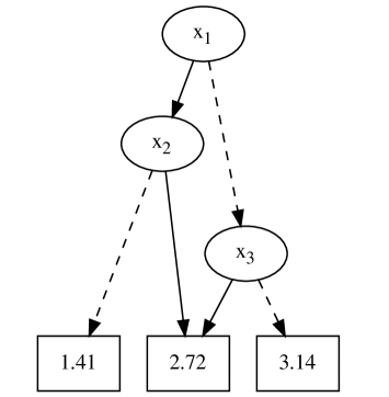
Figure 5: The directed graph $G$ of an ADD with variable set $X=\left\{x_{1},x_{2},x_{3}\right\}$, carrier set $S=\mathbb{R}$, and diagram variable order $\pi(x_{i})=i$ for $i=1,2,3$. If an edge from an oval node is solid (respectively dashed), then the corresponding Boolean variable is assigned 1 (respectively 0).

Appendix 0.C Proofs

0.C.1 Proof of Theorem 2.1

Proof

For every $\tau\in 2^{(X\cup Y)\setminus\left\{x\right\}}$, we have:

$$\left(\sum_{x}(A\cdot B)\right) (\tau)=(A\cdot B)(\tau)+(A\cdot B)(\tau\cup\left\{x\right\})$$ (Definition 2)

$$=A(\tau\cap X)\cdot B(\tau\cap Y)+A((\tau\cup\left\{x\right\})\cap X)\cdot B((\tau\cup\left\{x\right\})\cap Y)$$ (Definition 1)

$$=A(\tau\cap X)\cdot B(\tau\cap Y)+A((\tau\cup\left\{x\right\})\cap X)\cdot B(\tau\cap Y) x\notin Y$$ (as )

$$=A(\tau\cap X)\cdot B(\tau\cap Y)+A(\tau\cap X\cup\left\{x\right\})\cdot B(\tau\cap Y) x\in X$$ (as )

$$=(A(\tau\cap X)+A(\tau\cap X\cup\left\{x\right\}))\cdot B(\tau\cap Y)$$

$$=\left(\sum_{x}A\right)(\tau\cap X)\cdot B(\tau\cap Y)$$ (Definition 2)

$$=\left(\sum_{x}A\right)(\tau\cap(X\setminus\left\{x\right\}))\cdot B(\tau\cap Y) x\notin\tau$$ (as )

$$=\left(\left(\sum_{x}A\right)\cdot B)\right)(\tau)$$ (Definition 1)

∎

0.C.2 Proof of Theorem 3.1

In this section, for pseudo-Boolean functions $f:2^{X}\to\mathbb{R}$, we define $\texttt{Vars}(f)\equiv X$. Notice that a clause $c$ in a CNF formula can be interpreted as a Boolean function $c:2^{\texttt{Vars}(c)}\to\left\{0,1\right\}$. Similarly, a set $\varphi$ of clauses can be interpreted as the Boolean function $\varphi=\prod_{c\in\varphi}c$.

Let $X$ be a set of variables and $W=\prod_{x\in X}W_{x}$ be a literal-weight function. Given a set $Y\subseteq X$, we define $W_{Y}\equiv\prod_{x\in Y}W_{x}$. Notice $W_{Y}\cdot W_{Z}=W_{Y\cup Z}$ for all sets $Y,Z\subseteq X$.

Let $\varphi$ be a CNF formula over a set $X$ of variables, $(T,r,\gamma,\sigma)$ be a project-join tree of $\varphi$, and $n\in\mathcal{V}(T)$. Denote by $S(n)$ the subtree rooted at $n$. We define the set $\Phi(n)$ of clauses that correspond to the leaves of $S(n)$:

$$\Phi(n)\equiv\begin{cases}\left\{\gamma(n)\right\}&\text{if }n\in\mathcal{L}(T)\\ \bigcup_{o\in\mathcal{C}(n)}\Phi(o)&\text{otherwise}\end{cases}$$

We also define the set $P(n)$ of all variables to project in the subtree $S(n)$:

$$P(n)\equiv\begin{cases}\varnothing&\text{if }n\in\mathcal{L}(T)\\ \pi(n)\cup\bigcup_{o\in\mathcal{C}(n)}P(o)&\text{otherwise}\end{cases}$$

Lemma 1

In a project-join tree $(T,r,\gamma,\pi)$, let $n$ be an internal node with children $o\neq q$. Then $P(o)\cap\texttt{Vars}\left(\Phi(q)\cdot W_{P(q)}\right)=\varnothing$.

Proof

Let variable $x\in P(o)$. Notice that $x\in\pi(s)$ for some internal node $s$ that is a descendant of $o$. Assume there is an arbitrary clause $c\in\varphi$ s.t. $x$ appears in $c$. By the last property in Definition 4, the corresponding leaf $\gamma^{-1}(c)$ is a descendant of $s$ and thus a descendant of $o$. So $x$ appears in no descendant leaf of $q$ (as $q$ is a sibling of $o$ in the tree $T$). Thus $x\notin\texttt{Vars}(\Phi(q))$.

Now, note that $P(q)\subseteq\texttt{Vars}(\Phi(q))$, again by Definition 4. So $x\notin P(q)$. Therefore $x\notin\texttt{Vars}(\Phi(q)\cdot W_{P(q)})=\texttt{Vars}(\Phi(q))\cup\texttt{Vars}(W_{P(q)})=\texttt{Vars}(\Phi(q))\cup P(q)$. Since $x\in P(o)$ is arbitrary, we have $P(o)\cap\texttt{Vars}\left(\Phi(q)\cdot W_{P(q)}\right)=\varnothing$. ∎

Lemma 2

In a project-join tree $(T,r,\gamma,\pi)$, let $n$ be an internal node with children $o\neq q$. Then:

$$\sum_{P(o)}\left(\Phi(o)\cdot W_{P(o)}\right)\cdot\sum_{P(q)}\left(\Phi(q)\cdot W_{P(q)}\right)=\sum_{P(o)\cup P(q)}\left(\Phi(o)\Phi(q)\cdot W_{P(o)\cup P(q)}\right)$$

Proof

We have:

$$\sum_{P(o)}\left(\Phi(o)\cdot W_{P(o)}\right)\cdot\sum_{P(q)}\left(\Phi(q)\cdot W_{P(q)}\right) =\sum_{P(o)}\left(\Phi(o)\cdot W_{P(o)}\cdot\sum_{P(q)}\left(\Phi(q)\cdot W_{P(q)}\right)\right) P(o)$$ (undoing early projection of , observing Lemma 1)

$$=\sum_{P(q)}\sum_{P(o)}\left(\Phi(o)\cdot W_{P(o)}\cdot\Phi(q)\cdot W_{P(q)}\right) P(q)$$ (undoing early projection of , observing Lemma 1)

$$=\sum_{P(o)}\sum_{P(q)}\left(\Phi(o)\Phi(q)\cdot W_{P(o)}W_{P(q)}\right)$$

$$=\sum_{P(o)\cup P(q)}\left(\Phi(o)\Phi(q)\cdot W_{P(o)\cup P(q)}\right)$$

∎

Lemma 3

Let $\varphi$ be a CNF formula over a set $X$ of variables, $W$ be a literal-weight function over $X$, and $(T,r,\gamma,\pi)$ be a project-join tree of $\varphi$. Then for every node $n$ in $T$:

$$f^{W}_{n}=\sum_{P(n)}\left(\Phi(n)\cdot W_{P(n)}\right)$$

Proof

Notice that both pseudo-Boolean functions have the same variables in their domains:

$$\texttt{Vars}\left(f^{W}_{n}\right) =\texttt{Vars}(n)$$

$$=\texttt{Vars}(\Phi(n))\setminus P(n)$$

$$=\texttt{Vars}\left(\sum_{P(n)}\left(\Phi(n)\cdot W_{P(n)}\right)\right)$$

We employ structural induction on $n\in\mathcal{V}(T)$. In the base case, $n$ is a leaf. So $P(n)=\varnothing$ and $\Phi(n)=\left\{\gamma(n)\right\}$. We have:

$$f^{W}_{n} =\gamma(n)$$ (Equation (2))

$$=\prod_{c\in\Phi(n)}c$$ (singleton set)

$$=\Phi(n)$$

$$=\Phi(n)\cdot\prod_{x\in\varnothing}W_{x} 1$$ (an empty product is equal to the number )

$$=\Phi(n)\cdot W_{\varnothing}$$

$$=\Phi(n)\cdot W_{P(n)}$$

$$=\sum_{\varnothing}\left(\Phi(n)\cdot W_{P(n)}\right)$$ (convention on projection)

$$=\sum_{P(n)}\left(\Phi(n)\cdot W_{P(n)}\right)$$

In the inductive case, $n$ is an internal node of $T$. Our induction hypothesis is that

$$f^{W}_{o}=\sum_{P(o)}\left(\Phi(o)\cdot W_{P(o)}\right)$$

for every child node $o$ of $n$. Then we have:

$$f^{W}_{n} =\sum_{\pi(n)}\left(\prod_{o\in\mathcal{C}(n)}f^{W}_{o}\cdot\prod_{x\in\pi(n)}W_{x}\right)$$ (Equation (2))

$$=\sum_{\pi(n)}\left(\prod_{o\in\mathcal{C}(n)}f^{W}_{o}\cdot W_{\pi(n)}\right)$$

$$=\sum_{\pi(n)}\left(\prod_{o\in\mathcal{C}(n)}\left(\sum_{P(o)}\left(\Phi(o)\cdot W_{P(o)}\right)\right)\cdot W_{\pi(n)}\right)$$ (induction hypothesis)

$$=\sum_{\pi(n)}\left(\sum_{\bigcup_{s\in\mathcal{C}(n)}P(s)}\left(\prod_{o\in\mathcal{C}(n)}\Phi(o)\cdot W_{\bigcup_{t\in\mathcal{C}(n)}P(t)}\right)\cdot W_{\pi(n)}\right)$$ (applying Lemma 2 multiple times)

$$=\sum_{\pi(n)}\left(\sum_{\bigcup_{s\in\mathcal{C}(n)}P(s)}\left(\prod_{o\in\mathcal{C}(n)}\Phi(o)\cdot W_{\bigcup_{t\in\mathcal{C}(n)}P(t)}\cdot W_{\pi(n)}\right)\right) \pi(n)\cap\bigcup_{s\in\mathcal{C}(n)}P(s)=\varnothing$$ (undoing early projection, observing )

$$=\sum_{\pi(n)\cup\bigcup_{s\in\mathcal{C}(n)}P(s)}\left(\prod_{o\in\mathcal{C}(n)}\Phi(o)\cdot W_{\bigcup_{t\in\mathcal{C}(n)}P(t)\cup\pi(n)}\right)$$

$$=\sum_{P(n)}\left(\prod_{o\in\mathcal{C}(n)}\Phi(o)\cdot W_{P(n)}\right) P(n)$$ (definition of )

$$=\sum_{P(n)}\left(\Phi(n)\cdot W_{P(n)}\right) \Phi(n)=\bigcup_{o\in\mathcal{C}(n)}\Phi(o)$$ (as is a set of clauses)

∎

Now, we can prove Theorem 3.1.

Proof

As $r$ is the root of the project-join tree, $P(r)=X$ and $\Phi(r)=\varphi$. Then:

$$f^{W}_{r}(\varnothing) =\left(\sum_{P(r)}\left(\Phi(r)\cdot W_{P(r)}\right)\right)(\varnothing)$$ (Lemma 3)

$$=\left(\sum_{X}\left(\varphi\cdot W_{X}\right)\right)(\varnothing)$$

$$=\left(\sum_{X}\left(\varphi\cdot W\right)\right)(\varnothing)$$

$$=W(\varphi)$$

∎

0.C.3 Proof of Theorem 4.1

In this section, we assume the antecedents of Theorem 4.1 regarding the functions ClusterVarOrder, ClauseRank, and ChosenCluster. Notice that for each $i=1,2,\ldots,m$ in Algorithm 1, we have the following:

• $\Gamma_{i}$ is a set of clauses

• $\kappa_{i}$ is a set of nodes that includes leaves $l$ s.t. $\gamma(l)\in\Gamma_{i}$

• $n_{i}$ is an internal node

• $n_{i}$’s children include the leaves in $\kappa_{i}$

• $\pi(n_{i})=X_{i}$

We show that the first property in Definition 4 holds:

Lemma 4 (Property 1)

The set $\left\{\pi(n):n\in\mathcal{V}(T)\setminus\mathcal{L}(T)\right\}$ is a partition of $X$.

Proof

For each $i=1,2,\ldots,m$, Algorithm 1 constructs an internal nodes $n_{i}$ with $\pi(n_{i})=X_{i}$. Recall that $\left\{X_{i}\right\}_{i=1}^{m}$ is a partition of $X$. Then $\left\{\pi(n_{i})\right\}_{i=1}^{m}$ is the same partition of $X$. ∎

We show that the second property in Definition 4 holds through the following lemmas.

Lemma 5

Let $1\leq p<q\leq m$. Assume some $x\in\texttt{Vars}(\Gamma_{p})\cap X_{q}$. Then $x\in\texttt{Vars}(n_{p})$.

Proof

Notice $x\in X_{q}=\pi(n_{q})$. Then $x$ is projected in $n_{q}$. Since $p<q$, we know $x$ is projected in neither $n_{p}$ nor a descendants of $n_{p}$. Since $x\in\texttt{Vars}(\Gamma_{p})$, we know $x$ remains in $n_{p}$. ∎

Lemma 6

Let $1\leq p_{0}<q\leq m$. Assume $\texttt{Vars}(\Gamma_{p_{0}})\cap X_{q}\neq\varnothing$. Then the internal node $n_{p_{0}}$ is a descendant of the node $n_{q}$.

Proof

Let $n_{p_{1}},n_{p_{2}},\ldots$ be the parent, grandparent,… of $n_{p_{0}}$. By way of contradiction, assume every $p_{i}\neq q$. Let $x$ be a variable in $\texttt{Vars}(\Gamma_{p_{0}})\cap X_{q}\neq\varnothing$. By Lemma 5, we know $x\in\texttt{Vars}(n_{p_{0}})$. Notice that for all $i=0,1,2,\ldots$, we have:

• $x\notin X_{p_{i}}$, as $x\in X_{q}$ already

• $x\in\texttt{Vars}(n_{p_{i}})$, as $x$ remains from $n_{p_{0}}$ without being projected according to $\pi(n_{p_{i}})=X_{p_{i}}$

• $p_{i}<p_{i+1}=\texttt{ChosenCluster}(n_{p_{i}})\leq q$ by Condition 3 of Theorem 4.1, as $x\in\pi(n_{q})\cap\texttt{Vars}(n_{p_{i+1}})=X_{q}\cap\texttt{Vars}(n_{p_{i+1}})\neq\varnothing$

So the strictly increasing sequence $\langle p_{i}\rangle_{i}$ must contain $q$, contradiction. ∎

Lemma 7

Let $1\leq p,q\leq m$. Assume $\texttt{Vars}(\Gamma_{p})\cap X_{q}\neq\varnothing$. Then $p\leq q$.

Proof

To the contrary, assume $p>q$. Then by construction, $X_{q}\cap\texttt{Vars}(\Gamma_{p})=\varnothing$, contradiction. ∎

Lemma 8 (Property 2)

Let $1\leq q\leq m$ and variable $x\in\pi(n_{q})$. Take an arbitrary clause $c\in\varphi$ s.t. $x\in\texttt{Vars}(c)$. Then the leaf $\gamma^{-1}(c)$ is a descendant of $n_{q}$.

Proof

Notice that $c\in\Gamma_{p}$ for some $1\leq p\leq m$. Then $x\in\texttt{Vars}(c)\subseteq\texttt{Vars}(\Gamma_{p})$. Note that $x\in\pi(n_{q})=X_{q}$. Thus $p\leq q$ by Lemma 7.

Let $l=\gamma^{-1}(c)$. Notice that $l\in\kappa_{p}$ (as $c\in\Gamma_{p}$). So $l$ is a child of the node $n_{p}$.

• If $p=q$, then $l$ is a child of $n_{q}$, and we are done.

• If $p<q$, by Lemma 6, we know $n_{p}$ is a descendant of $n_{q}$, as $x\in\texttt{Vars}(\Gamma_{p})\cap\pi(n_{q})=\texttt{Vars}(\Gamma_{p})\cap X_{q}\neq\varnothing$. Then $l$ is a descendant of $n_{q}$.

∎

Now we can prove Theorem 4.1

Proof

Algorithm 1 returns a tree $T$ with root $n_{m}$, bijection $\gamma:\mathcal{L}(T)\to\varphi$, and labeling function $\pi:\mathcal{V}(T)\setminus\mathcal{L}(T)\to 2^{X}$. The project-join tree properties are satisfied, by Lemma 4 and Lemma 8 ∎

0.C.4 Proof of Theorem 4.2

Let $(T,r,\gamma,\pi)$ be the object returned by Algorithm 2. We first observe that $T$ is indeed a tree with root $r$. For each node $a\in\mathcal{V}(T)$, let $O(a)\in\mathcal{V}(S)$ denote the node in $\mathcal{V}(S)$ s.t. $a$ was created in the $\texttt{Process}(O(a),\ell)$ call for some $\ell\subseteq X$. Throughout, let $s$ denote the value obtained on Line 2 of Algorithm 2.

We begin by stating three basic properties of Algorithm 2.

Lemma 9

For each $a\in\mathcal{V}(T)\setminus\mathcal{L}(T)$, we have $\pi(a)\subseteq\chi(O(a))$.

Proof

This follows from Line 2 of Algorithm 2. ∎

Lemma 10

For each $a\in\mathcal{V}(T)\setminus\mathcal{L}(T)$ where $O(a)\neq s$, let $p$ be the parent of $O(a)$ in $S$. Then $\pi(a)\cap\chi(p)=\varnothing$.

Proof

Observe that $\ell=\chi(p)$ in the $\texttt{Process}(O(a),\ell)$ call on Line 2. The result then follows from Line 2 of Algorithm 2. ∎

Lemma 11

Let $n\in\mathcal{V}(S)$. For every $\ell\subseteq X$ and $i\in\texttt{Process}(n,\ell)$, we have $\texttt{Vars}(i)\subseteq\ell$.

Proof

We proceed by induction on the tree structure of $S$.

Let $A$ denote the set $children$ after Line 2 occurs and let $a\in A$. We first prove that $\texttt{Vars}(a)\subseteq\chi(n)$. First, assume that $a$ is a leaf node corresponding to some $c\in clauses$. In this case, $\texttt{Vars}(a)=\texttt{Vars}(c)\subseteq\chi(n)$ by Line 2. Otherwise $a\in\texttt{Process}(o,\chi(n))$ for some $o\in C(n)$. In this case, notice that $n$ is an internal node, so by the inductive hypothesis, $\texttt{Vars}(a)\subseteq\chi(n)$.

Now, if $A=\varnothing$, then $\texttt{Process}(n,\ell)$ returns $\varnothing$, so the lemma is vacuously true. If $\chi(n)\subseteq\ell$, then $A$ is returned by $\texttt{Process}(n,\ell)$. So for every $i\in A$, we have $\texttt{Vars}(i)\subseteq\chi(n)\subseteq\ell$.

Otherwise, $A\neq\varnothing$ and $\chi(n)\not\subseteq\ell$. In this case, $\texttt{Process}(n,\ell)$ returns a single node $i$ with $\texttt{Vars}(i)=\cup_{a\in A}\texttt{Vars}(a)\setminus(\chi(n)\setminus\ell)\subseteq\chi(n)\setminus(\chi(n)\setminus\ell)\subseteq\ell$. ∎

Given these three properties, it is straightforward to prove that $(T,r,\gamma,\pi)$ satisfies all conditions to be a project-join tree of $\varphi$. We prove each condition in a separate lemma here.

Lemma 12

$\gamma$ is a bijection.

Proof

Note that $\gamma$ is an injection since $found$ on Line 2 of Algorithm 2 ensures that we generate at most one leaf node for each clause. To show that $\gamma$ is a surjection, consider $c\in\varphi$. Then $\texttt{Vars}(c)$ forms a clique in the Gaifman graph of $\varphi$. It follows (since the treewidth of a complete graph on $k$ vertices is $k-1$) that $\texttt{Vars}(c)\subseteq\chi(n)$ for some $n\in\mathcal{V}(S)$. Thus $\gamma$ is a surjection as well. ∎

Lemma 13

$P=\{\pi(a):a\in\mathcal{V}(T)\setminus\mathcal{L}(T)\}$ is a partition of $X$.

Proof

First, let $x\in X$. Then $x\in\texttt{Vars}(c)$ for some $c\in\varphi$. Since $\gamma$ is a bijection, $x\in\texttt{Vars}(p)$ for some $p=\gamma^{-1}(c)\in\mathcal{L}(T)$. However, by Lemma 11, we know $x\notin\texttt{Vars}(r)=\varnothing$. Thus $x$ must have been projected out at some node $q\in\mathcal{V}(T)$ between $p$ and $r$. It follows that $x\in\pi(q)\subseteq P$.

On the other hand, assume for the sake of a contradiction that there are distinct $a,b\in\mathcal{V}(T)$ s.t. $x\in\pi(a)\cap\pi(b)$. By Lemma 9, $x\in\chi(O(a))\cap\chi(O(b))$. Since $S$ is a tree, there is some node $p\in\mathcal{V}(S)$ on the path between $O(a)$ and $O(b)$ s.t. $p$ is the parent of either $O(a)$ or $O(b)$. By Property 3 of tree decompositions, $x\in\chi(p)$. However, this contradicts Lemma 10. ∎

Lemma 14

For each internal node $a\in\mathcal{V}(T)\setminus\mathcal{L}(T)$, variable $x\in\pi(a)$, and clause $c\in\varphi$ s.t. $x$ appears in $c$, the leaf node $\gamma^{-1}(c)$ is a descendant of $a$ in $T$.

Proof

If $O(a)=s$, then $a$ is the root of $T$, so all leaf nodes are descendants. Otherwise, assume for the sake of contradiction that $\gamma^{-1}(c)$ is not a descendant of $a$ in $T$. Then $O(\gamma^{-1}(c))$ is not a descendant of $O(a)$ in $S$. This means that the parent $p\in\mathcal{V}(S)$ of $O(a)$ is on the path between $O(a)$ and $O(\gamma^{-1}(c))$. By Lemma 9, we must have $x\in\chi(O(a))\cap\chi(O(\gamma^{-1}(c)))$. By Property 3 of tree decompositions, $x\in\chi(p)$. But this contradicts Lemma 10. ∎

It follows that $(T,r,\gamma,\pi)$ is a project-join tree of $\varphi$.

0.C.5 Proof of Theorem 4.3

Proof

Let $X=\texttt{Vars}(\varphi)$. Define $\chi:\mathcal{V}(T)\to 2^{X}$ by, for all $n\in\mathcal{V}(T)$, $\chi(n)\equiv\texttt{Vars}(n)$ if $n\in\mathcal{L}(T)$ and $\chi(n)\equiv\texttt{Vars}(n)\cup\pi(n)$ otherwise. Then $(T,\chi)$ is a tree decomposition of the Gaifman graph of $\varphi$. Moreover, the width of $(T,\chi)$ is $\texttt{tw}(T,\chi)=\max_{n\in\mathcal{V}(T)}\left|\chi(n)\right|-1=\max_{n\in\mathcal{V}(T)}\texttt{size}(n)-1=w-1$. ∎

References

- [1] Abseher, M., Musliu, N., Woltran, S.: htd–a free, open-source framework for (customized) tree decompositions and beyond. In: CPAIOR. pp. 376–386. Springer (2017), https://doi.org/10.1007/978-3-319-59776-8_30
- [2] Aguirre, A.S.M., Vardi, M.: Random 3-SAT and BDDs: the plot thickens further. In: CP. pp. 121–136. Springer (2001), https://doi.org/10.1007/3-540-45578-7_9
- [3] Arad, I., Landau, Z.: Quantum computation and the evaluation of tensor networks. SICOMP 39(7), 3089–3121 (2010), https://doi.org/10.1137/080739379
- [4] Bacchus, F., Dalmao, S., Pitassi, T.: Solving #SAT and Bayesian inference with backtracking search. JAIR 34, 391–442 (2009), https://doi.org/10.1613/jair.2648
- [5] Bahar, R.I., Frohm, E.A., Gaona, C.M., Hachtel, G.D., Macii, E., Pardo, A., Somenzi, F.: Algebraic decision diagrams and their applications. Form Method Syst Des 10(2-3), 171–206 (1997), https://doi.org/10.1023/A:1008699807402
- [6] Baumgartner, G., Auer, A., Bernholdt, D.E., Bibireata, A., Choppella, V., Cociorva, D., Gao, X., Harrison, R.J., Hirata, S., Krishnamoorthy, S., et al.: Synthesis of high-performance parallel programs for a class of ab initio quantum chemistry models. IEEE 93(2), 276–292 (2005), https://doi.org/10.1109/JPROC.2004.840311
- [7] Bellman, R.: Dynamic programming. Science 153(3731), 34–37 (1966), https://doi.org/10.1126/science.153.3731.34
- [8] Bouquet, F.: Gestion de la dynamicité et énumération d’impliquants premiers: une approche fondée sur les Diagrammes de Décision Binaire. Ph.D. thesis, Aix-Marseille 1 (1999), https://www.theses.fr/1999AIX11011
- [9] Burch, J.R., Clarke, E.M., Long, D.E.: Symbolic model checking with partitioned transition relations. In: VLSI. pp. 49–58 (1991), http://citeseerx.ist.psu.edu/viewdoc/summary?doi=10.1.1.23.1932
- [10] Burchard, J., Schubert, T., Becker, B.: Laissez-faire caching for parallel #SAT solving. In: SAT. pp. 46–61. Springer (2015), https://doi.org/10.1007/978-3-319-24318-4_5
- [11] Charwat, G., Woltran, S.: BDD-based dynamic programming on tree decompositions. Tech. rep., Technische Universität Wien, Institut für Informationssysteme (2016), https://dbai.tuwien.ac.at/research/report/dbai-tr-2016-95.pdf
- [12] Chavira, M., Darwiche, A.: Compiling Bayesian networks using variable elimination. In: IJCAI. pp. 2443–2449 (2007), https://dl.acm.org/doi/10.5555/1625275.1625669
- [13] Cichocki, A.: Era of big data processing: a new approach via tensor networks and tensor decompositions. arXiv preprint arXiv:1403.2048 (2014), https://arxiv.org/abs/1403.2048
- [14] Cichocki, A., Mandic, D., De Lathauwer, L., Zhou, G., Zhao, Q., Caiafa, C., Phan, H.A.: Tensor decompositions for signal processing applications: from two-way to multiway component analysis. IEEE SPM 32(2), 145–163 (2015), https://doi.org/10.1109/MSP.2013.2297439
- [15] Clarke, E., Biere, A., Raimi, R., Zhu, Y.: Bounded model checking using satisfiability solving. Form Method Syst Des 19(1), 7–34 (2001), https://doi.org/10.1023/A:1011276507260
- [16] Dal, G.H., Laarman, A.W., Lucas, P.J.: Parallel probabilistic inference by weighted model counting. In: PGM. pp. 97–108 (2018), http://proceedings.mlr.press/v72/dal18a.html
- [17] Dalmau, V., Kolaitis, P.G., Vardi, M.Y.: Constraint satisfaction, bounded treewidth, and finite-variable logics. In: CP. pp. 310–326. Springer (2002), https://doi.org/10.1007/3-540-46135-3_21
- [18] Darwiche, A.: Dynamic jointrees. In: UAI. pp. 97–104 (1998), https://dl.acm.org/doi/10.5555/2074094.2074106
- [19] Darwiche, A.: New advances in compiling CNF to decomposable negation normal form. In: ECAI. pp. 318–322 (2004), https://dl.acm.org/doi/10.5555/3000001.3000069
- [20] Dechter, R.: Bucket elimination: a unifying framework for reasoning. AIJ 113(1-2), 41–85 (1999), https://doi.org/10.1016/S0004-3702(99)00059-4
- [21] Dechter, R.: Constraint processing. Morgan Kaufmann (2003), https://doi.org/10.1016/B978-1-55860-890-0.X5000-2
- [22] Dechter, R., Pearl, J.: Tree clustering for constraint networks. AIJ 38(3), 353–366 (1989), https://doi.org/10.1016/0004-3702(89)90037-4
- [23] van Dijk, T., van de Pol, J.: Sylvan: multi-core decision diagrams. In: TACAS. pp. 677–691. Springer (2015), https://doi.org/10.1007/978-3-662-46681-0_60
- [24] Domshlak, C., Hoffmann, J.: Probabilistic planning via heuristic forward search and weighted model counting. JAIR 30, 565–620 (2007), https://dl.acm.org/doi/10.5555/1622637.1622652
- [25] Dudek, J.M., Dueñas-Osorio, L., Vardi, M.Y.: Efficient contraction of large tensor networks for weighted model counting through graph decompositions. arXiv preprint arXiv:1908.04381 (2019), https://arxiv.org/abs/1908.04381
- [26] Dudek, J.M., Phan, V.H.N., Vardi, M.Y.: ADDMC: weighted model counting with algebraic decision diagrams. In: AAAI. vol. 34, pp. 1468–1476 (2020), https://doi.org/10.1609/aaai.v34i02.5505
- [27] Dudek, J.M., Vardi, M.Y.: Parallel weighted model counting with tensor networks. In: MCW (2020), https://mccompetition.org/assets/files/2020/MCW˙2020˙paper˙1.pdf
- [28] Evenbly, G., Pfeifer, R.N.: Improving the efficiency of variational tensor network algorithms. Physical Review B 89(24), 245118 (2014), https://doi.org/10.1103/PhysRevB.89.245118
- [29] Fargier, H., Marquis, P., Niveau, A., Schmidt, N.: A knowledge compilation map for ordered real-valued decision diagrams. In: AAAI (2014), https://dl.acm.org/doi/10.5555/2893873.2894036
- [30] Fatahalian, K., Sugerman, J., Hanrahan, P.: Understanding the efficiency of GPU algorithms for matrix-matrix multiplication. In: SIGGRAPH/EUROGRAPHICS. pp. 133–137 (2004), https://doi.org/10.1145/1058129.1058148
- [31] Fichte, J.K., Hecher, M., Thier, P., Woltran, S.: Exploiting database management systems and treewidth for counting. In: PADL. pp. 151–167. Springer (2020), https://doi.org/10.1007/978-3-030-39197-3_10
- [32] Fichte, J.K., Hecher, M., Zisser, M.: An improved GPU-based SAT model counter. In: CP. pp. 491–509. Springer (2019), https://doi.org/10.1007/978-3-030-30048-7_29
- [33] Gogate, V., Domingos, P.: Approximation by Quantization. In: UAI. pp. 247–255 (2011), https://dl.acm.org/doi/10.5555/3020548.3020578
- [34] Gomes, C.P., Sabharwal, A., Selman, B.: Model counting. Handbook of Satisfiability 20 (2009), https://doi.org/10.3233/978-1-58603-929-5-633
- [35] Hoey, J., St-Aubin, R., Hu, A., Boutilier, C.: SPUDD: stochastic planning using decision diagrams. In: UAI. pp. 279–288 (1999), https://arxiv.org/abs/1301.6704
- [36] Jégou, P., Kanso, H., Terrioux, C.: Improving exact solution counting for decomposition methods. In: ICTAI. pp. 327–334. IEEE (2016), https://doi.org/10.1109/ICTAI.2016.0057
- [37] Kask, K., Dechter, R., Larrosa, J., Dechter, A.: Unifying tree decompositions for reasoning in graphical models. AIJ 166(1-2), 165–193 (2005), https://doi.org/10.1016/j.artint.2005.04.004
- [38] Kjolstad, F., Kamil, S., Chou, S., Lugato, D., Amarasinghe, S.: The tensor algebra compiler. PACMPL 1(OOPSLA), 1–29 (2017), https://doi.org/10.1145/3133901
- [39] Klebanov, V., Manthey, N., Muise, C.: SAT-based analysis and quantification of information flow in programs. In: QEST. pp. 177–192 (2013), https://doi.org/10.1007/978-3-642-40196-1_16
- [40] Kolaitis, P.G., Vardi, M.Y.: Conjunctive-query containment and constraint satisfaction. JCSS 61(2), 302–332 (2000), https://doi.org/10.1006/jcss.2000.1713
- [41] Koriche, F., Lagniez, J.M., Marquis, P., Thomas, S.: Knowledge compilation for model counting: affine decision trees. In: IJCAI (2013), https://dl.acm.org/doi/10.5555/2540128.2540265
- [42] Koster, A.M., Bodlaender, H.L., Van Hoesel, S.P.: Treewidth: computational experiments. Electron Notes Discrete Math 8, 54–57 (2001), https://doi.org/10.1016/S1571-0653(05)80078-2
- [43] Kourtis, S., Chamon, C., Mucciolo, E., Ruckenstein, A.: Fast counting with tensor networks. SciPost Phys 7(5) (2019), https://doi.org/10.21468/SciPostPhys.7.5.060
- [44] Kwiatkowska, M., Norman, G., Parker, D.: Stochastic model checking. In: SFM. pp. 220–270. Springer (2007), https://doi.org/10.1007/978-3-540-72522-0_6
- [45] Lagniez, J.M., Marquis, P.: Preprocessing for propositional model counting. In: AAAI (2014), https://dl.acm.org/doi/10.5555/2892753.2892924
- [46] Lagniez, J.M., Marquis, P.: An improved decision-DNNF compiler. In: IJCAI. pp. 667–673 (2017), https://doi.org/10.24963/ijcai.2017/93
- [47] Lawson, C.L., Hanson, R.J., Kincaid, D.R., Krogh, F.T.: Basic linear algebra subprograms for Fortran usage. TOMS 5(3), 308–323 (1979), https://doi.org/10.1145/355841.355847
- [48] McMahan, B.J., Pan, G., Porter, P., Vardi, M.Y.: Projection pushing revisited. In: EDBT. pp. 441–458. Springer (2004), https://doi.org/10.1007/978-3-540-24741-8_26
- [49] Morgenstern, A., Schneider, K.: From LTL to symbolically represented deterministic automata. In: VMCAI. pp. 279–293. Springer (2008), https://doi.org/10.1007/978-3-540-78163-9_24
- [50] Naveh, Y., Rimon, M., Jaeger, I., Katz, Y., Vinov, M., s Marcu, E., Shurek, G.: Constraint-based random stimuli generation for hardware verification. AI Magazine 28(3), 13–13 (2007), https://dl.acm.org/doi/10.5555/1597122.1597129
- [51] Oliphant, T.E.: A guide to NumPy, vol. 1. Trelgol Publishing USA (2006), https://dl.acm.org/doi/book/10.5555/2886196
- [52] Oztok, U., Darwiche, A.: A top-down compiler for sentential decision diagrams. In: IJCAI (2015), https://dl.acm.org/doi/10.5555/2832581.2832687
- [53] Palacios, H., Geffner, H.: Compiling uncertainty away in conformant planning problems with bounded width. JAIR 35, 623–675 (2009), https://dl.acm.org/doi/10.5555/1641503.1641518
- [54] Pan, G., Vardi, M.Y.: Symbolic techniques in satisfiability solving. J Autom Reasoning 35(1-3), 25–50 (2005), https://doi.org/10.1007/s10817-005-9009-7
- [55] Robertson, N., Seymour, P.D.: Graph minors. X. Obstructions to tree-decomposition. J Combinatorial Theory B 52(2), 153–190 (1991), https://doi.org/10.1016/0095-8956(91)90061-N
- [56] Samer, M., Szeider, S.: Algorithms for propositional model counting. J Discrete Algorithms 8(1), 50–64 (2010), https://doi.org/10.1007/978-3-540-75560-9_35
- [57] Samer, M., Szeider, S.: Constraint satisfaction with bounded treewidth revisited. JCSS 76(2), 103–114 (2010), https://doi.org/10.1016/j.jcss.2009.04.003
- [58] Sang, T., Bacchus, F., Beame, P., Kautz, H.A., Pitassi, T.: Combining component caching and clause learning for effective model counting. SAT 4, 20–28 (2004), http://www.satisfiability.org/SAT04/accepted/65.html
- [59] Sang, T., Beame, P., Kautz, H.A.: Performing Bayesian inference by weighted model counting. In: AAAI. vol. 1, pp. 475–482. AAAI Press (2005), https://dl.acm.org/doi/10.5555/1619332.1619409
- [60] Shachter, R.D., Andersen, S.K., Szolovits, P.: Global conditioning for probabilistic inference in belief networks. In: UAI, pp. 514–522. Elsevier (1994), https://doi.org/10.1016/B978-1-55860-332-5.50070-5
- [61] Sinz, C., Kaiser, A., Küchlin, W.: Formal methods for the validation of automotive product configuration data. AI EDAM 17(1), 75–97 (2003), https://doi.org/10.1017/S0890060403171065
- [62] Smilde, A., Bro, R., Geladi, P.: Multi-way analysis: applications in the chemical sciences. John Wiley & Sons (2005), https://doi.org/10.1002/0470012110
- [63] Somenzi, F.: CUDD: CU decision diagram package–release 3.0.0. University of Colorado at Boulder (2015), https://github.com/ivmai/cudd
- [64] Strasser, B.: Computing tree decompositions with FlowCutter: PACE 2017 submission. arXiv preprint arXiv:1709.08949 (2017), https://arxiv.org/abs/1709.08949
- [65] Tabajara, L.M., Vardi, M.Y.: Factored Boolean functional synthesis. In: FMCAD. pp. 124–131. IEEE (2017), https://dl.acm.org/doi/10.5555/3168451.3168480
- [66] Tamaki, H.: Positive-instance-driven dynamic programming for treewidth. J Comb Optim 37(4), 1283–1311 (2019), https://doi.org/10.1007/s10878-018-0353-z
- [67] Tarjan, R.E., Yannakakis, M.: Simple linear-time algorithms to test chordality of graphs, test acyclicity of hypergraphs, and selectively reduce acyclic hypergraphs. SICOMP 13(3), 566–579 (1984), https://doi.org/10.1137/0213035
- [68] Uribe, T.E., Stickel, M.E.: Ordered binary decision diagrams and the Davis-Putnam procedure. In: CCL. pp. 34–49. Springer (1994), https://doi.org/10.1007/BFb0016843
- [69] Valiant, L.G.: The complexity of enumeration and reliability problems. SICOMP 8(3), 410–421 (1979), https://doi.org/10.1137/0208032