Gluonic Hot Spot Initial Conditions in Heavy-Ion Collisions

Abstract

The initial conditions in heavy-ion collisions are calculated in many different frameworks. The importance of nucleon position fluctuations within the nucleus and sub-nucleon structure has been established when modeling initial conditions for input to hydrodynamic calculations. However, there remain outstanding puzzles regarding these initial conditions, including the measurement of the near equivalence of the elliptical $v_{2}$ and triangular $v_{3}$ flow coefficients in ultra-central 0-1% Pb$+$Pb collisions at the LHC. Recently a calculation termed magma incorporating gluonic hot spots via two-point correlators in the Color Glass Condensate framework, and no nucleons, provided a simultaneous match to these flow coefficients measured by the ATLAS experiment, including in ultra-central 0-1% collisions. Our calculations reveal that the magma initial conditions do not describe the experimental data when run through full hydrodynamic sonic simulations or when the hot spots from one nucleus resolve hot spots from the other nucleus, as predicted in the Color Glass Condensate framework. We also explore alternative initial condition calculations and discuss their implications.

I Introduction

The physics underlying the first fraction of a fm/$c$ in heavy-ion collisions is of fundamental interest in its own right, while also a necessary input in order to extract properties of the created quark-gluon plasma (QGP) that evolves from this initial state Heinz and Snellings (2013); Romatschke and Romatschke (2019). There are innumerable modelings of the said initial state ranging from claimed ab initio calculations to phenomenological parameterizations Albacete and Marquet (2014); Lappi (2009); Miller et al. (2007). A major advance in the field more than a decade ago was the incorporation of nucleon position fluctuations via Monte Carlo Glauber calculations Miller et al. (2007) and subsequently the realization that odd flow coefficients would be non-zero Alver and Roland (2010). Most recently it has become clear that sub-nucleon structure is necessary to understand data in proton-proton and proton-nucleus collisions M$\ddot{\rm a}$ntysaari et al. (2017); Romatschke and Romatschke (2019), as well as collisions of deformed nuclei such as Uranium-Uranium Adamczyk et al. (2015).

Monte Carlo Glauber code including nucleon and constituent quarks is now publicly available Loizides (2016). Such calculations have been incorporated into multiple frameworks, including the often used trento Moreland et al. (2015) model. In this framework, each incoming nucleon or sub-nucleon is modeled via a two-dimensional Gaussian distribution and the deposited energy is proportional to the square root of the local projectile density times the local target density (in the trento $p=0$ mode). Another such framework is ip-jazma Nagle and Zajc (2019), where the deposited energy can be chosen as the product of local projectile density times the local target density or the square root, as in the trento model. Both examples are purely phenomenological; in fact, the trento model has been used in Bayesian analyses in an attempt to constrain the initial state parameters Bernhard et al. (2019). A recent comparison of these scalings for multiplicity distributions is detailed in Ref. Carzon et al. (2020a).

In contrast, in the weakly-coupled limit, one can in principle calculate the initial conditions in the so-called Color Glass Condensate (CGC) framework (also referred to as the saturation framework) – for useful reviews see Refs. Gelis (2013); Gelis et al. (2010); Venugopalan . Although the calculation is termed ab initio, it is an effective theory in the limit as the coupling $\alpha_{s}$ goes to zero and for high gluon occupation number, and thus its applicability in the heavy-ion collision regime at RHIC and the LHC is unclear. Regardless, within this framework one can assume the projectile and target nuclear color charge densities are described by a local saturation scale $Q_{s}$ and then the deposited energy is proportional to the product of the projectile and target color charge densities Lappi (2006); Romatschke and Romatschke (2019). It is notable that as derived in Ref. Romatschke and Romatschke (2019), this simple product is also the result for the deposited energy in the strongly-coupled limit. The ip-glasma code Schenke et al. (2012) provides a Monte Carlo framework for the calculation of initial conditions via this CGC effective theory. The calculation starts with Monte Carlo Glauber with nucleons or sub-nucleons and then associates a local saturation scale with a two-dimensional Gaussian distribution for each. Additional color charge fluctuations are included on the scale of the lattice spacing within the calculation. Finally, the deposited energy is calculated. The ip-glasma code also time evolves the initial color distribution using the Yang-Mills equations of motion, and this moderates the dependence of the additional color charge fluctuations on the lattice spacing. The ip-glasma initial conditions have been successful at matching experimental flow data when used as input to viscous hydrodynamic calculations – see for example Refs. Schenke et al. (2020, 2011).

The ip-jazma phenomenological model Nagle and Zajc (2019) was constructed to specifically evaluate initial conditions from the MSTV calculations for small collisions systems which are calculated in the so-called dilute-dense limit of the CGC framework Mace et al. (2019, 2018). ip-jazma can also calculate initial conditions as the simple product of two-dimensional target and projectile Gaussian distributions, the so-called dense-dense limit. These calculations provide an almost identical match to the energy deposit initial conditions from the full ip-glasma framework – see details in Appendix A. This agreement emphasizes that the key ingredients for the initial geometry are nucleons or sub-nucleons, Gaussian profiles, and taking the local product of these Gaussians. Features in the ip-glasma model from color domains or “spiky” local fluctuations are sub-dominant, and thus not confirmed by agreement with flow data. We highlight that the ip-glasma model also calculates the early pre-hydrodynamic time evolution, often up to $\tau=0.4~{}\mathrm{fm}/c$, and this is not modeled in ip-jazma or trento. The evaluation of this pre-hydrodynamic time evolution and its apples-to-apples comparison with free streaming or strongly-coupled dynamics is a topic for another paper.

A new approach was recently put forward also within the CGC framework, termed magma Gelis et al. (2019). A recent analysis comparing various models including magma is given in Ref. Floerchinger et al. (2020). In the following sections we (a) detail the magma calculation and reproduce their results, (b) show results from magma initial conditions run through full hydrodynamic sonic simulations, (c) show how the magma results change if hot spots from one nucleus interact with hot spots from the other nucleus – which is not the default in the magma framework, and finally (d) detail results from alternative initial condition calculations.

II magma Calculation

In the magma framework, each nucleus is modeled as a two-dimensional profile of color charge density calculated within the CGC framework. The density is built from localized color charges. What is notable is that these color charges are distributed without any modeling of nucleons, and are only bounded by the total size of the nucleus, characterized by the Woods-Saxon parameters for a Pb nucleus ($R=6.62$ fm and $a=0.55$ fm). The number of localized color charges used in the magma calculation is approximately 100 per nuclei, and thus about half the number of nucleons. The authors highlight that this is distinct from the ip-glasma calculation, where they first distribute the 208 nucleons from the Pb nucleus, and then calculate the saturation momentum depending on the nucleon positions. It is unclear what physics justification allows for neglecting nucleons for heavy-ion collisions at these energies.

Another distinguishing feature is that what is calculated in magma is the energy deposit from localized color charges from the projectile Pb nucleus striking a smooth target nucleus, and then linearly summing the energy deposit from localized color charges from the target Pb nucleus striking a smooth projectile Pb nucleus. This is nicely visualized in Figure 1 from the magma paper Gelis et al. (2019) – we have regenerated a version of this representation here as Figure 1, with the resulting energy deposit shown in the upper right panel. Each interaction creates a sharply peaked energy deposit that decreases as the distance squared. The calculation reproduced the one-point and two-point functions of the energy density field calculation in the CGC effective theory Albacete et al. (2019). We thus label the magma calculation as “$A\times B_{WS}+B\times A_{WS}$”, which is in striking contrast from the ip-glasma “$A\times B$” calculation for the local energy density with two nuclei $A$ and $B$, with the resulting energy deposit shown in the lower right panel of Figure 1.

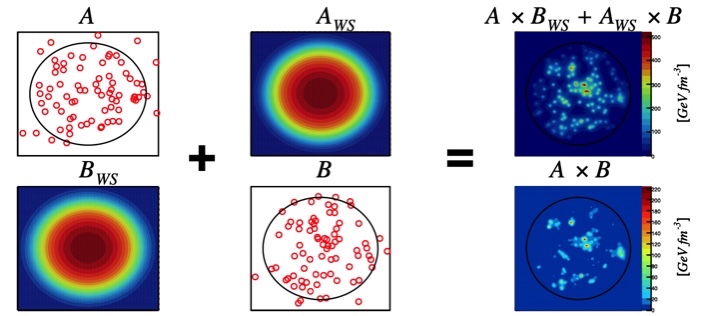
Figure 1: A schematic display of the initial energy deposition calculation. The hot spots in nucleus A are multiplied by the smooth distribution of nucleus B, labeled as $B_{WS}$ and summed with the inverse, hot spots in nucleus B multiplied by the smooth distribution of nucleus A. The resulting energy spatial distribution is shown on the top right plot. In contrast, the bottom right plot shows the $A\times B$ calculation using the modified magma code.

Using the publicly available Python code from the magma authors, we have reproduced their main result, as shown in Figure 2. The top panel shows the Pb+Pb energy deposit distribution in arbitrary units. The distribution is dividing into percentiles and then the geometric eccentricities are calculated within the individual centrality selections. This procedure is not identical to the method of centrality selection in experiment, though we expect this to have negligible impact on our conclusions. The second- and fourth- cumulants are calculated for the $n=2$ and $n=3$ flow harmonics as follows.

$$\varepsilon_{2}\{2\}=\sqrt{\left<\varepsilon_{2}^{2}\right>}$$ (1)

$$\varepsilon_{2}\{4\}=(2\left<\varepsilon_{2}^{2}\right>^{2}-\left<\varepsilon_{2}^{4}\right>)^{1/4}$$ (2)

$$\varepsilon_{3}\{2\}=\sqrt{\left<\varepsilon_{3}^{2}\right>}$$ (3)

In order to compare with experimental data, one takes advantage of the fact that hydrodynamics gives an approximately linear relationship between the final flow coefficient and the initial spatial anisotropy (e.g. $v_{2}\{2\}=\kappa_{2}\times\varepsilon_{2}\{2\}$, $v_{2}\{4\}=\kappa_{2}\times\varepsilon_{2}\{4\}$, and $v_{3}\{2\}=\kappa_{3}\times\varepsilon_{3}\{2\}$). We note that this ignores potential contributions from non-linear response Betz et al. (2017), a point we will discuss in the next section. The $\kappa_{2}$, $\kappa_{3}$ values depend in detail on the QGP properties such as the shear viscosity to entropy density ratio ($\eta$/S) and the treatment of hadronic re-scattering after hydrodynamic expansion. However, one can assume that these values to vary modestly with collision centrality, and thus they are fitted to experimental data after which one can examine the centrality dependence. We highlight that the $\kappa$ values are numerically determined by matching the experimental data at centrality = 20, and this is done in a consistent manner in the later comparisons in the paper. A single value of $\kappa_{2}$ determines the scaling for both the $v_{2}\{2\}$ and $v_{2}\{4\}$. Values for $\kappa_{2}=0.32$ and $\kappa_{3}=0.31$ are obtained, in good agreement with the numbers quoted in Ref. Gelis et al. (2019).

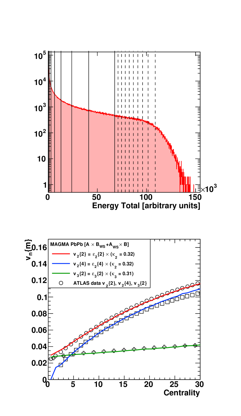
Figure 2: Initial condition calculation with magma. (Top) The total energy deposit distribution over one million events. Solid (dashed) vertical lines correspond to 10% (top 1%) percentiles. (Bottom) The $\varepsilon_{2}\{2\}$, $\varepsilon_{2}\{4\}$, and $\varepsilon_{3}\{2\}$ values as a function of centrality selection, scaled up by the respective $\kappa_{2,3}$ values. In comparison, ATLAS experiment data are shown for $v_{2}\{2\}$, $v_{2}\{4\}$, and $v_{3}\{2\}$.

Figure 2 (above) also shows the experimental data for $v_{2}\{2\}$, $v_{2}\{4\}$, and $v_{3}\{2\}$ as measured by the ATLAS experiment Aaboud et al. (2020). The ATLAS measurements are from charged particles in $0.5<p_{T}<5~{}\mathrm{GeV}$ and $|\eta|<2.5$ with a requirement of a minimum pseudorapidity gap of 1.67 units. The agreement between the magma results and the experimental data is excellent, noting particularly the splitting between $v_{2}\{2\}$ and $v_{2}\{4\}$. Also remarkable is the agreement with both $v_{2}\{2\}$ and $v_{3}\{2\}$ up to the most central 0-1% Pb+Pb collisions. Figure 3 shows the ratio of $\kappa_{3}\times\varepsilon_{3}\{2\}$ / $\kappa_{2}\times\varepsilon_{2}\{2\}$ as a function of collision centrality for both data and the magma calculation. The ratio in data (and from magma) approaches unity which encapsulates the ultra-central flow puzzle.

In the limit of impact parameter $b=0$ Pb+Pb collisions, the average geometry is circularly symmetric and all spatial anisotropies are zero, i.e. $\varepsilon_{n}=0$. However, with random fluctuations, for example from nucleon position fluctuations, one obtains non-zero eccentricities but where all moments are approximately equal, i.e. $\varepsilon_{2}\approx\varepsilon_{3}\approx\varepsilon_{4}\approx...\approx\varepsilon_{n}$ Mocsy and Sorensen (2011). However, even in this case, in general the translation of initial geometry into flow is less efficient for higher moments and thus one would expect $\kappa_{3}$ is less than $\kappa_{2}$ – in contradistinction to the $\kappa_{2,3}$ values obtained in the magma fit. For a recent discussion of this puzzle, see Ref. Carzon et al. (2020b). We explore this translation of geometry to flow quantitatively in the next section.

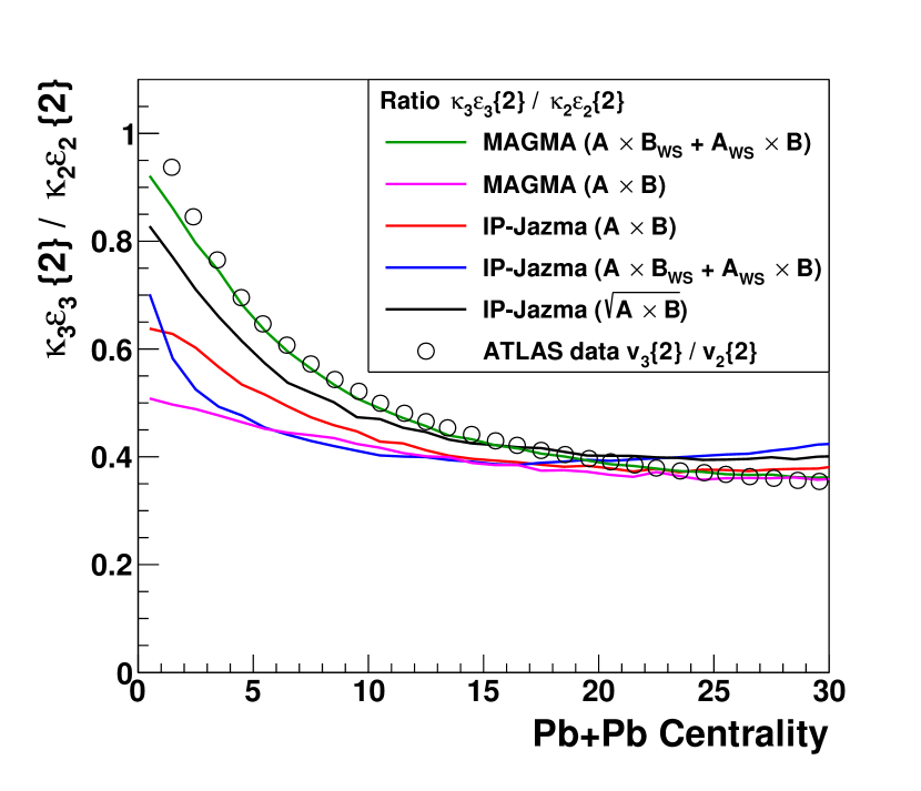
Figure 3: Ratio of $v_{3}\{2\}/v_{2}\{2\}$ as a function of Pb$+$Pb collision centrality as measured by the ATLAS experiment. Multiple theoretical calculations are also shown.

III Full hydrodynamic calculations

The linear factors $\kappa_{2,3}$ can be determined either phenomenologically by matching calculated $\varepsilon_{n}$ to measured $v_{n}$ (as is done in the magma result shown above) or can be calculated directly with viscous hydrodynamics or parton kinetic theory as examples. It is striking in the magma calculation that $\kappa_{2}\approx\kappa_{3}$; i.e. the elliptic and triangular flow have the same linear response coefficient. In general, even in the case of small viscous damping, e.g. shear viscosity to entropy density $\eta/s=1/4\pi$, the response coefficient is expected to be smaller for higher moments, i.e. larger $n$ values. This feature has also been seen in parton transport calculations Alver and Roland (2010). We can test this specifically for the 0-1% Pb$+$Pb collision initial conditions from magma.

To this end, we have run 1000 such magma initial conditions for events all falling into the 0-1% centrality selection through a full hydrodynamic simulation including hadronic cascade afterburner B3D using the publicly available sonic code Romatschke (2015). Figure 4 shows time snapshots of the two-dimensional temperature profile from a single magma initial condition through hydrodynamic evolution. The sonic running conditions for the hydrodynamic stage include shear viscosity to entropy density $\eta$/S $=1/4\pi$ and bulk viscosity to entropy density $\zeta/s=0$. The hydrodynamic initial time is set to $\tau_{0}=0.4$ fm/c and the freeze-out temperature is set to $T_{f}=170$ MeV.

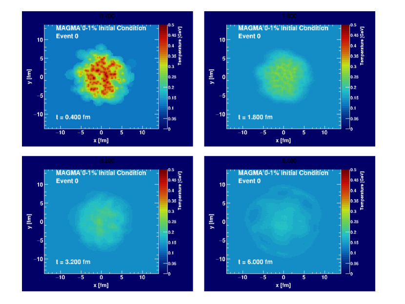
Figure 4: Time evolution event display for a Pb$+$Pb 0-1% most central collision using magma initial conditions run through sonic viscous hydrodynamics. The time snapshots show the temperature in the transverse (x,y) plane and are at $t=0.4,1.8,3.2,6.0$ fm/c.

In Figures 5 and 6, we plot for Pb$+$Pb centralities 0-1% and 25-26%, respectively, the flow coefficients $v_{2}$ (upper) and $v_{3}$ (lower) for three different $p_{T}$ selections versus the magma initial geometry $\varepsilon_{2}$ and $\varepsilon_{3}$ for 1000 individual events. One sees a reasonable linear relationship in all cases as indicated via the calculated Pearson coefficients shown in the legend. Each panel is fit to a line with the intercept forced at zero and the slope corresponding to the $\kappa_{n}$ value. It is noticeable that for the 25-26% centrality events, where the events extend out to larger values of $\varepsilon_{2}$ there is a clear non-linearity contribution - which is reasonably described by a quadratic fit. Another observation is that the Pearson coefficients are significantly lower for the $v_{3}$ in the 25-26% centrality compared with the 0-1% centrality, i.e. there is a lot more event-to-event spread around the central linear relation. Lastly, the $\kappa_{n}$ values increase with increasing $p_{T}$. Since the $\varepsilon_{n}$ values for each event do not depend on particle $p_{T}$, this increase is simply a reflection of the larger $v_{n}$ as a function of $p_{T}$. We highlight that in general any linear approximation of flow coefficients with eccentricities is not known to be valid for $p_{T}$-differential anisotropies and thus integrating over a finite $p_{T}$ range introduces a sensitivity on the infrared-cut used Luzum (2011).

Figure 7 shows for Pb$+$Pb collisions of 0-1% (left) and 25-26% (right) centralities the $\kappa_{2}$ (upper) and $\kappa_{3}$ (middle) coefficients and their ratio (lower) as a function of charged hadron $p_{T}$. The $\kappa_{2}$ and $\kappa_{3}$ $p_{T}$-integrated values over the range 0.5 - 3.0 GeV are shown as solid horizontal lines. The lower $p_{T}$ selection is made to match the ATLAS measurement range and the upper $p_{T}$ selection is nearing the limit where the hydrodynanic calculations has significant systematic uncertainties. The values for Pb$+$Pb 0-1% centrality are $\kappa_{2}=0.38$ and $\kappa_{3}=0.28$, and for Pb$+$Pb 25-26% centrality are $\kappa_{2}=0.28$ and $\kappa_{3}=0.24$. Thus, the assumption used in the magma comparison in Figures 2 and  3 of $\kappa_{n}$ independent of centrality is significantly in error. It is also notable that the ratio of $\kappa_{3}/\kappa_{2}$ varies between these two centrality selections, 0.73 (0-1%) and 0.85 (25-26%). Both of these values are substantially lower than the 0.31/0.32 = 0.97 obtained from the magma fit shown in Figure 2.

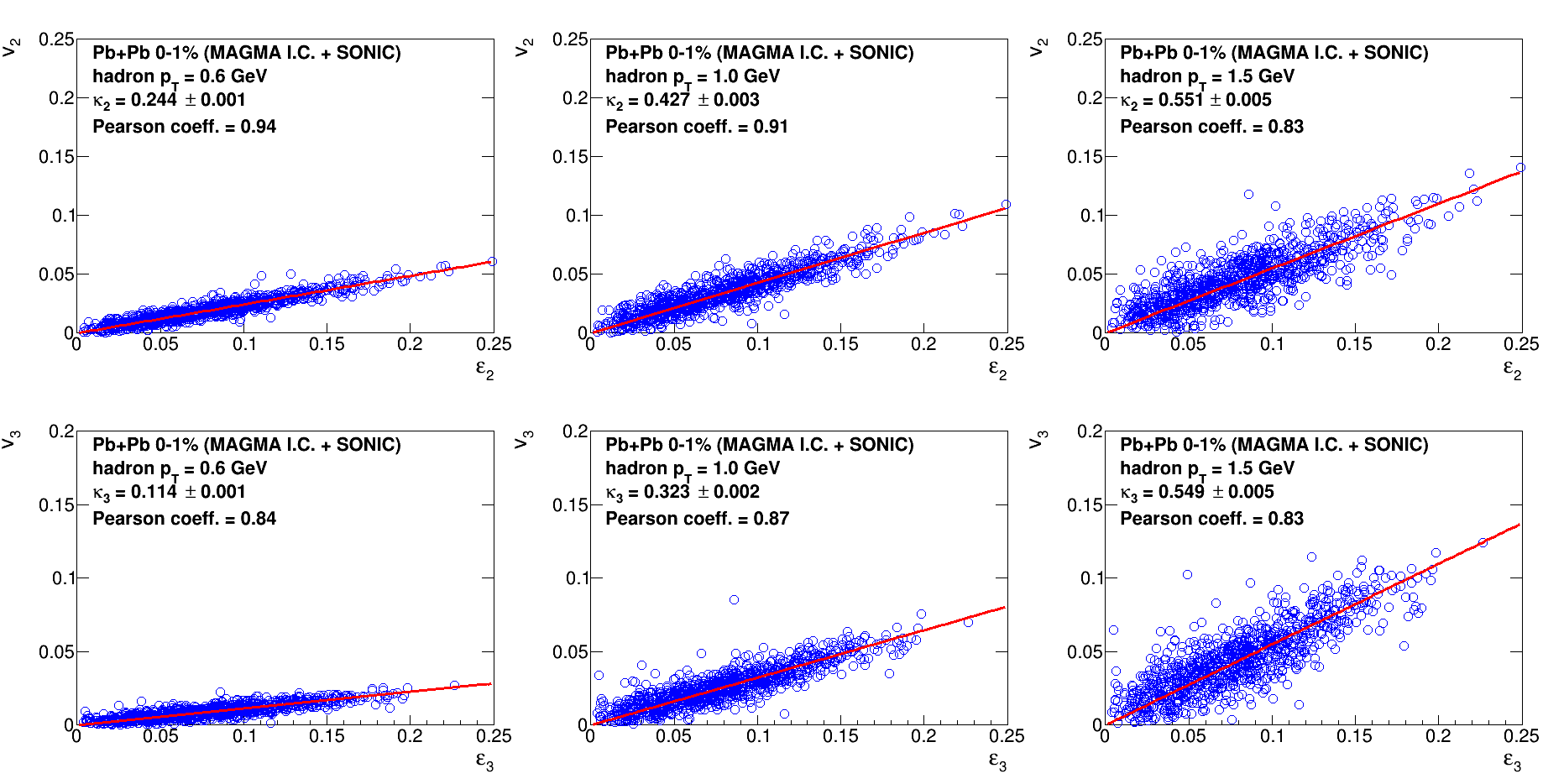
Figure 5: Results from sonic hydrodynamic calculations for magma initial condition 0-1% central Pb+Pb collisions. Shown are results in the upper (lower) panels from individual events for $v_{2}$ ($v_{3}$) versus the initial geometric $\varepsilon_{2}$ ($\varepsilon_{3}$). The linear fits represent the $\kappa$ response coefficients. Also shown are the Pearson coefficients indicating the degree of linear correlation.

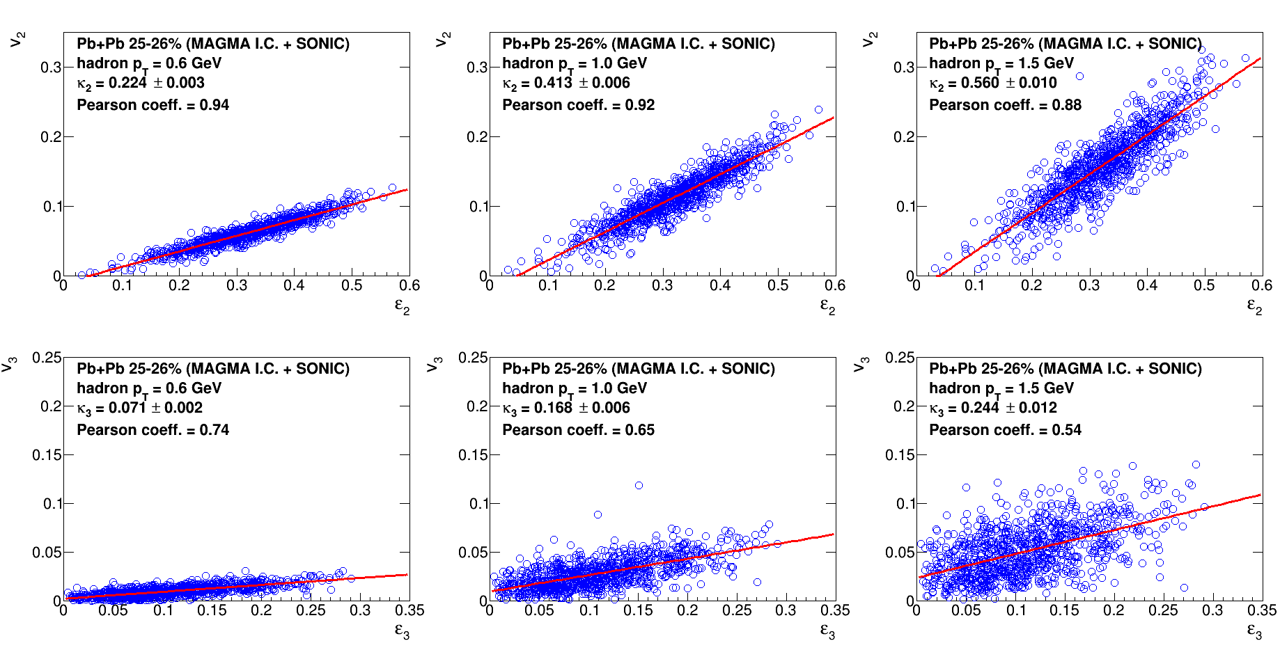
Figure 6: Results from sonic hydrodynamic calculations for magma initial condition 25-26% central Pb+Pb collisions. Shown are results in the upper (lower) panels from individual events for $v_{2}$ ($v_{3}$) versus the initial geometric $\varepsilon_{2}$ ($\varepsilon_{3}$). The linear fits represent the $\kappa$ response coefficients. Also shown are the Pearson coefficients indicating the degree of linear correlation.

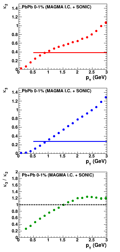
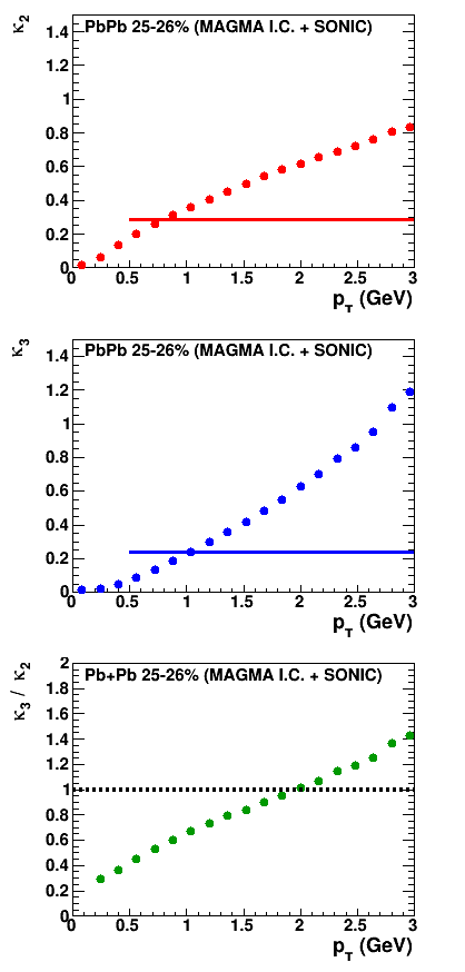
Figure 7: Results from sonic hydrodynamic calculations for magma initial condition 0-1% (left) and 25-26% (right) Pb+Pb collisions. Shown are results in the upper (middle) panels are the $\kappa_{2}$ ($\kappa_{3}$) values as a function of charged hadron $p_{T}$. The horizontal line represented the $p_{T}$-integrated value over the range 0.5 - 3.0 GeV. The lower panel shows the ratio of $\kappa_{3}/\kappa_{2}$ as a function of $p_{T}$. The dashed line is set at one for reference.

We have mapped out the $\kappa_{n}$ values over the full centrality range 0-30% corresponding to charged hadrons with $p_{T}=0.5-3.0$ GeV as shown in Figure 8. The open red (blue) points correspond to the mean $\kappa_{2}$ ($\kappa_{3}$) values. In the inset, we show the event-by-event distribution of $\kappa_{3}$ values for the specific Pb+Pb 5-6% centrality. There is a non-Gaussian high-side tail which is dominated by events with very small values of $\varepsilon_{3}$. We have also fit these distributions to a Gaussian and shown the Gaussian mean values in Figure 8 as closed points. There is a clear and substantial centrality dependence for both $\kappa_{2}$ and $\kappa_{3}$ values. The method for comparison of measured $v_{2}\{2\}$ with $\kappa_{2}\times\varepsilon_{2}\{2\}$ for example, used in the magma analysis in Figure 2, would be technically more comparable to extracting $\kappa_{2}$ from the sonic hydrodynamic calculation as the RMS of $v_{n}$ divided by the RMS of $\varepsilon_{n}$. These values are also shown in Figure 8 and are only very modestly different from the Gaussian mean values.

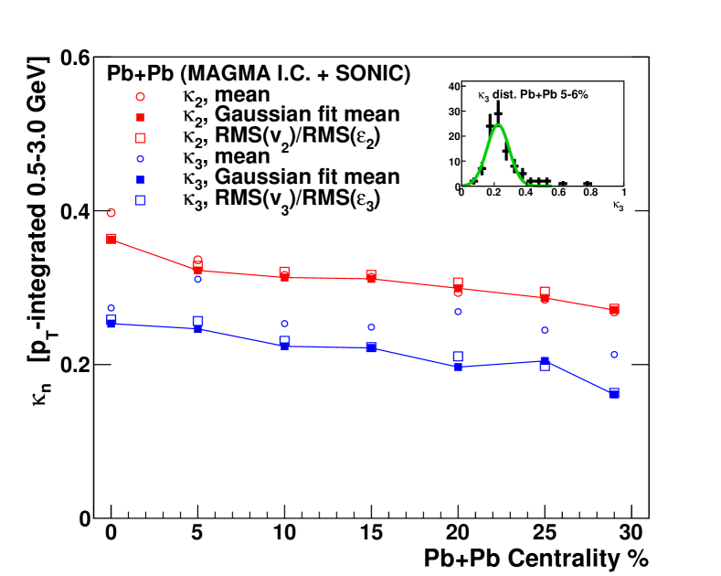
Figure 8: Results from sonic hydrodynamic calculations for magma initial condition 0-30% Pb+Pb collisions quantifying the $\kappa{2}$ and $\kappa_{3}$ values both via the mean values and the Gaussian fit mean values. Also shown are values of $\kappa_{n}$ determined as the RMS of $v_{n}$ divided by the RMS of $\varepsilon_{n}$. An example fit is shown in the inset.

We have also run calculations with nearly ideal hydrodynamics $\eta/s=0.02=1/4\times 1/4\pi$ and find for Pb$+$Pb 0-1% centrality value of $\kappa_{2}=0.53$ and $\kappa_{3}=0.36$. These are significantly higher than the values quoted above for $\eta/$S = $1/4\pi$ as expected since there is less viscous damping and hence stronger flow. Shown in Figure 9 is a comparison of the $\kappa_{3}/\kappa_{2}$ ratio with two different values of $\eta/$S. There are modest difference that again highlight that medium properties do not completely cancel out in these ratios.

The testing of magma initial conditions with full hydrodynamics reveals that in fact the magma initial conditions do not match experimental data to resolve the ultra-central puzzle. Any resolution of the ultra-central puzzle from an initial geometry picture must be coupled with full transport calculations for confirmation.

Figure 9: Results from sonic hydrodynamic calculations for magma initial conditions 0-1% for the ratio $\kappa_{3}/\kappa_{2}$ for two different values of $\eta$/S.

IV Alternative magma Modeling

Next we test whether the magma results are highlight dependent on the non-standard $A\times B_{WS}+A_{WS}\times B$ calculation of energy deposit. To this end, we have modified the magma code to calculate the energy deposit as $A\times B$, more in line with the weakly-coupled ip-glasma calculation. Figure 10 shows the comparison of eccentricity and flow cumulants from the modified-magma calculation. The splitting between the $v_{2}\{2\}$ and $v_{2}\{4\}$ is no longer captured by the calculation. Also the agreement with both $v_{2}\{2\}$ and $v_{3}\{2\}$ is not maintained. These results plotted as the ratio of $v_{3}\{2\}$ / $v_{2}\{2\}$ are also shown in Figure 3 and the modified-magma calculation only reaches 0.5 in the most central events. Matching the experimental $v_{n}$ data, the new value for $\kappa_{3}=0.15$ is now much smaller than $\kappa_{2}=0.28$. The original magma calculation has a larger contribution from the intrinsic geometry, encapsulated in the smooth nuclear distribution, compared to fluctuations. This modified magma calculation has relatively larger geometry fluctuations and thus the $v_{2}$ has a flatter centrality dependence and the relative scaling to match $v_{2}$ and $v_{3}$ are very different. Thus, the magma results are very sensitive to this non-standard calculation of energy deposit, and do not match experimental data using the more standard $A\times B$ method.

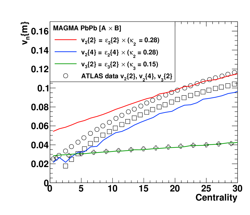
Figure 10: Initial condition calculation with magma but modified to run where the energy deposit is proportional to $A\times B$. The $\varepsilon_{2}\{2\}$, $\varepsilon_{2}\{4\}$, and $\varepsilon_{3}\{2\}$ values as a function of centrality selection are scaled up by the respective $\kappa_{2,3}$ values. In comparison, ATLAS experiment data are shown for $v_{2}\{2\}$, $v_{2}\{4\}$, and $v_{3}\{2\}$.

V Alternative Initial Conditions

Within the ip-jazma framework, we can calculate initial conditions in a variety of modes. First, we show results in Figure 11, where the energy deposit is chosen to be proportional to the local energy density in the projectile times the local energy density in the target ($A\times B$ mode). As detailed in Appendix A, this models the initial spatial energy distribution in ip-glasma almost perfectly. The agreement with experimental data is reasonable, although there is more splitting between $v_{2}\{2\}$ and $v_{3}\{2\}$ in the calculation. Also, as shown as a ratio in Figure 3, this geometry does not resolve the ultra-central puzzle. Interestingly, the phenomenologically fitted $\kappa_{2}$ is now 50% larger than $\kappa_{3}$, more in line with hydrodynamic expectations. We highlight that this calculation is with nucleons as two-dimensional Gaussians, and ignores sub-nucleons. Sub-nucleon degrees of freedom in this context have been explored in Ref. Loizides (2016) and they do not resolve the ultra-central puzzle.

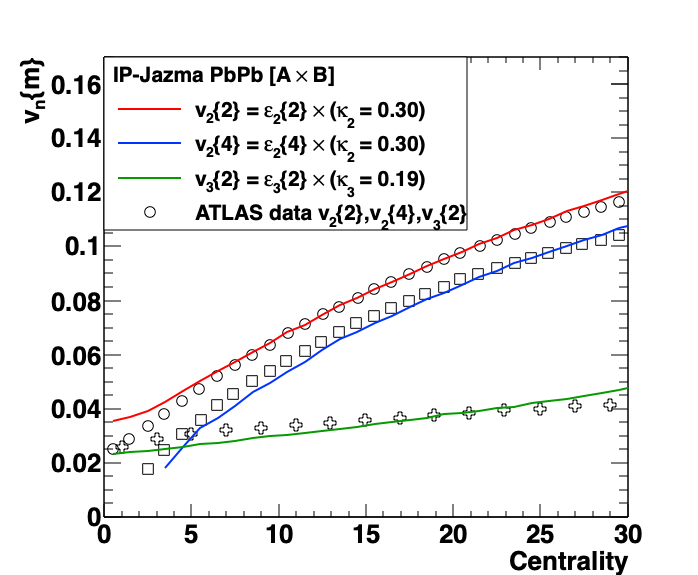
Figure 11: Initial condition calculation with ip-jazma run where the energy deposit is proportional to $A\times B$, as is true in the ip-glasma model. The $\varepsilon_{2}\{2\}$, $\varepsilon_{2}\{4\}$, and $\varepsilon_{3}\{2\}$ values as a function of centrality selection, scaled up by the respective $\kappa_{2,3}$ values. In comparison, ATLAS experiment data are shown for $v_{2}\{2\}$, $v_{2}\{4\}$, and $v_{3}\{2\}$.

Next, we show results in Figure 12, where the energy deposit is chosen to be proportional to the square root of the local energy density in the projectile times a smooth target nucleus summed with the local energy density in the target times a smooth projectile ($\sqrt{A\times B}$ as done in the trento calculation with $p=0$). The agreement with experimental data is quite good, though as shown in Figure 3, the results are still below the experimental data for $v_{3}\{2\}$ / $v_{2}\{2\}$. It is again notable that the $\kappa_{2}$ is approximately 50% larger than $\kappa_{3}$, more in line with hydrodynamic expectations. We note however that these $\kappa_{n}$ values have been extracted by fitting the entire 0-30% centrality range, and we know from full hydrodynamic simulations that $\kappa_{n}$ vary with centrality. Thus, a final evaluation can only be made with full hydrodynamic comparison to the data.

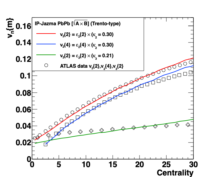
Figure 12: Initial condition calculation with ip-jazma run where the energy deposit is proportional to $\sqrt{A\times B}$ as is true in the trento model with parameter $p=0$. The $\varepsilon_{2}\{2\}$, $\varepsilon_{2}\{4\}$and $\varepsilon_{3}\{2\}$ values as a function of centrality selection, scaled up by the respective $\kappa_{2,3}$ values. In comparison, ATLAS experiment data are shown for $v_{2}\{2\}$, $v_{2}\{4\}$ and $v_{3}\{2\}$.

In both of these cases, it is important to run full hydrodynamic simulations and with variations on medium properties to have a precision test of the centrality dependence and whether the ultra-central puzzle is reconciled. Such simulations with sonic are underway.

VI Summary

In summary, we have reproduced the results from the magma initial condition model and its agreement with elliptic and triangular flow coefficients in Pb$+$Pb collisions at the LHC. However, we find that these results are highly dependent on the energy deposit being proportional to hot spots in the projectile hitting a smooth nuclear target and hot spots in the target hitting a smooth nuclear projectile, i.e. the hot spots do not “see” each other. In addition the translation factors $\kappa_{2,3}$ implied by the data comparison are in contradistinction from what we find with full sonic hydrodynamic simulations. A critical take away is that any precision test of initial geometry must be carried out with full evolution to flow coefficients. We have explored other initial condition modeling (e.g. ip-glasma, trento) within the ip-jazma framework and find the large triangular flow coefficient in ultra-central Pb$+$Pb collisions remains a puzzle requiring further investigation.

VII Appendix A

As detailed earlier, the ip-glasma is a first principles calculation in the CGC weakly-coupled limit. Focusing only on the initial distribution of energy deposit in the transverse plane, we find that there are no non-trivial manifestations of color domains or “spiky” fluctuations that have been confirmed by experiment through comparisons of flow measurements and initial conditions run through hydrodynamics. This is in line with studies on the lack of sensitivity to fine-scale structures in long-wavelength hydrodynamics Gardim et al. (2018). This observation is based on direct comparisons of calculated geometries between two models, ip-jazma and ip-glasma. As a brief reminder, the ip-jazma calculation has no quantum fluctuations and only has Gaussian distributions associated with nucleons and energy deposit proportional to $A\times B$. Using identical Monte Carlo Glauber initial conditions for Au$+$Au events at $b=0$, fed through the ip-jazma and ip-glasma calculations yield essentially identical $\varepsilon_{2-6}$ distributions – shown in Figure 13. We quantify this comparison for the second and third harmonics with the following values from ip-glasma (ip-jazma): $\left<\varepsilon_{2}\right>=0.104~{}(0.105)$, $\mathrm{RMS}_{2}=0.054~{}(0.054)$, Kurtosis${}_{2}=0.271~{}(0.302)$ and $\left<\varepsilon_{3}\right>=0.089~{}(0.091)$, $\mathrm{RMS}_{3}=0.047~{}(0.048)$, Kurtosis${}_{3}=-0.023~{}(-0.030)$. We highlight that in such comparisons it is essential to have the same Monte Carlo Glauber configuration. For example, the default ip-glasma code has a Glauber two-nucleon exclusion radius $d=0.8$ fm, which is twice larger than typical values and is unlikely to reflect hard-core repulsion between two nucleons. If the Monte Carlo Glauber configuration for ip-glasma and ip-jazma were different, one might mistakenly attribute that difference with the models rather than the inputs for the Monte Carlo Glauber.

Figure 13: Distributions of spatial eccentricities $\varepsilon_{2-6}$ from ip-glasma and ip-jazma for 1000 Monte Carlo Glauber Au$+$Au events of impact parameter $b=0$.

Another comparison of relevance is the two-point energy-energy correlator. Shown in the left panels of Figure 14 are energy deposit displays from ip-glasma (upper panel) and ip-jazma (lower panel) using an identical Monte Carlo Glauber Au$+$Au event at $b=0$. Right panels of Figure 14 show the correlator ($\left<\varepsilon_{1}\times\varepsilon_{2}\right>/(\left<\varepsilon_{1}\right>\left<\varepsilon_{2}\right>)$), integrated over many events, as a function of distance scale from the ip-glasma (upper panel) and ip-jazma (lower panel) calculations. One sees a large distance scale (approximately 6 fm) structure from the size of the nucleus and a narrower (approximately 1 fm) structure from nucleons both in ip-glasma and ip-jazma. Only the narrowest scale structure at $<0.05~{}\mathrm{fm}$ in the ip-glasma calculation is absent in the ip-jazma calculation – see the inset for a zoomed in view. This structure in ip-glasma scales linearly with the lattice spacing used in the calculation and is put in by hand. Again, it is notable that there is no visible evidence of color domains in the energy deposit structure. We note that this “spiky” structure gets washed out with the subsequent time evolution in the ip-glasma framework. ip-jazma is a model only for the initial energy density and does not perform a time evolution as ip-glasma does.

We have run the same comparison with sub-nucleon structure (for example with three constituent quarks) and then there appears another structure in both ip-glasma and ip-jazma (approximately 0.2–0.3 fm), indicating that smaller structures can be seen in principle. Again, they do not appear to reflect any CGC-specific physics.

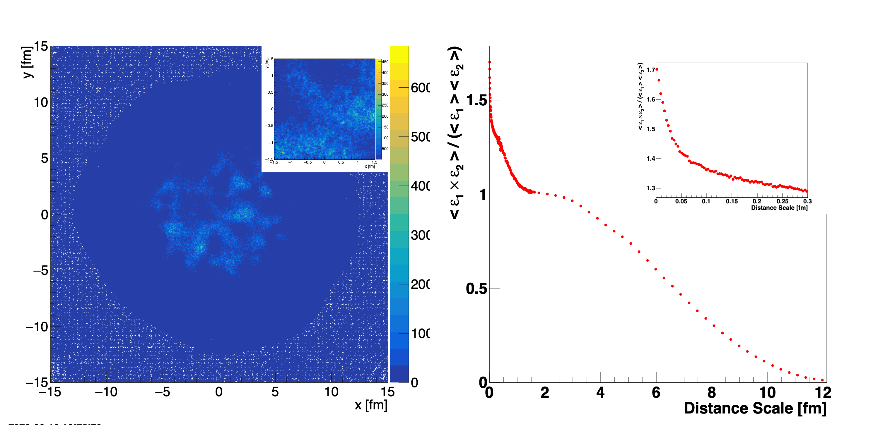
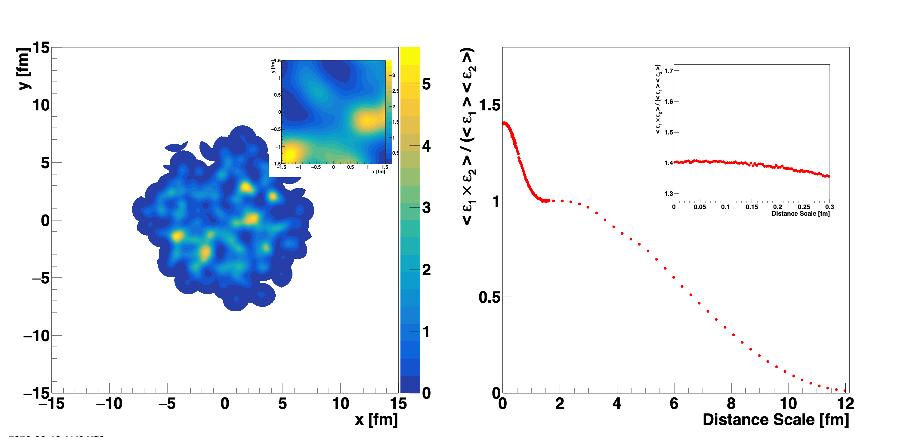
Figure 14: An identical Monte Carlo Glauber Au$+$Au event at $b=0$ fed through the ip-glasma (upper panel) and ip-jazma (lower panel) calculations. The energy density distributions are shown in the left panels, with a zoom inset for more detail. Also shown are the two-point energy-energy correlator averaged over many events in the ip-glasma (upper panel) and ip-jazma (lower panel) frameworks.

Lastly, we show a comparison of initial geometry from the ip-jazma calculation in a trento $p=0$ like mode. The results from ip-jazma with energy deposit proportional to $\sqrt{T_{A}\times T_{B}}$, i.e. the square root of the local nuclear thickness values, are shown in Figure 15. Since the energy distribution from each nucleon is distributed as a two-dimensional Gaussian, if one considers that one is taking the square root, i.e. $\sqrt{T_{A}}\times\sqrt{T_{B}}$, the Gaussian $\sigma$ should be increased by $\sqrt{2}$. However, one is locally summing the Gaussian contributions from all nucleons in a nucleus and then taking the square root, so there is no perfect match between trento $p=0$ style and ip-glasma style geometry.

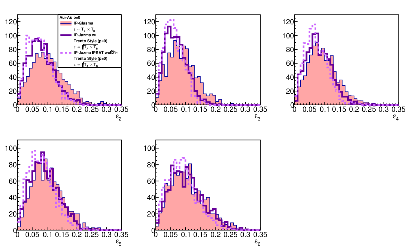
Figure 15: Distributions of spatial eccentricities $\varepsilon_{2-6}$ from ip-glasma and ip-jazma run with the trento-style energy deposit proportional to $\sqrt{T_{A}\times T_{B}}$ (i.e. $p=0$ trento mode) for 1000 Monte Carlo Glauber Au$+$Au events of impact parameter $b=0$. ip-jazma results where the two-dimensional Gaussian width is adjusted by $\sqrt{2}$ are also shown.

References

- Heinz and Snellings (2013) Ulrich Heinz and Raimond Snellings, “Collective flow and viscosity in relativistic heavy-ion collisions,” Ann. Rev. Nucl. Part. Sci. 63, 123–151 (2013), arXiv:1301.2826 [nucl-th] .
- Romatschke and Romatschke (2019) Paul Romatschke and Ulrike Romatschke, Relativistic Fluid Dynamics In and Out of Equilibrium, Cambridge Monographs on Mathematical Physics (Cambridge University Press, 2019) arXiv:1712.05815 [nucl-th] .
- Albacete and Marquet (2014) J.L. Albacete and C. Marquet, “Gluon saturation and initial conditions for relativistic heavy ion collisions,” Progress in Particle and Nuclear Physics 76, 1 – 42 (2014).
- Lappi (2009) T. Lappi, “Initial conditions of heavy ion collisions and high energy factorization,” Acta Phys. Polon. B 40, 1997–2012 (2009), arXiv:0904.1670 [hep-ph] .
- Miller et al. (2007) Michael L. Miller, Klaus Reygers, Stephen J. Sanders, and Peter Steinberg, “Glauber modeling in high energy nuclear collisions,” Ann. Rev. Nucl. Part. Sci. 57, 205–243 (2007), arXiv:nucl-ex/0701025 .
- Alver and Roland (2010) B. Alver and G. Roland, “Collision geometry fluctuations and triangular flow in heavy-ion collisions,” Phys. Rev. C 81, 054905 (2010), [Erratum: Phys.Rev.C 82, 039903 (2010)], arXiv:1003.0194 [nucl-th] .
- Mntysaari et al. (2017) Heikki Mntysaari, Bjrn Schenke, Chun Shen, and Prithwish Tribedy, “Imprints of fluctuating proton shapes on flow in proton-lead collisions at the LHC,” Phys. Lett. B772, 681–686 (2017), arXiv:1705.03177 [nucl-th] .
- Adamczyk et al. (2015) L. Adamczyk et al. (STAR), “Azimuthal anisotropy in UU and AuAu collisions at RHIC,” Phys. Rev. Lett. 115, 222301 (2015), arXiv:1505.07812 [nucl-ex] .
- Loizides (2016) Constantin Loizides, “Glauber modeling of high-energy nuclear collisions at the subnucleon level,” Phys. Rev. C 94, 024914 (2016), arXiv:1603.07375 [nucl-ex] .
- Moreland et al. (2015) J. Scott Moreland, Jonah E. Bernhard, and Steffen A. Bass, “Alternative ansatz to wounded nucleon and binary collision scaling in high-energy nuclear collisions,” Phys. Rev. C 92, 011901 (2015), arXiv:1412.4708 [nucl-th] .
- Nagle and Zajc (2019) J.L. Nagle and W.A. Zajc, “Assessing saturation physics explanations of collectivity in small collision systems with the IP-Jazma model,” Phys. Rev. C 99, 054908 (2019), arXiv:1808.01276 [nucl-th] .
- Bernhard et al. (2019) Jonah E. Bernhard, J. Scott Moreland, and Steffen A. Bass, “Bayesian estimation of the specific shear and bulk viscosity of quark–gluon plasma,” Nature Phys. 15, 1113–1117 (2019).
- Carzon et al. (2020a) Patrick Carzon, Matthew D. Sievert, and Jacquelyn Noronha-Hostler, “Importance of Multiplicity Fluctuations in Entropy Scaling,” (2020) arXiv:2007.12977 [nucl-th] .
- Gelis (2013) F. Gelis, “Color Glass Condensate and Glasma,” Int. J. Mod. Phys. A 28, 1330001 (2013), arXiv:1211.3327 [hep-ph] .
- Gelis et al. (2010) Francois Gelis, Edmond Iancu, Jamal Jalilian-Marian, and Raju Venugopalan, “The color glass condensate,” Annual Review of Nuclear and Particle Science 60, 463–489 (2010), https://doi.org/10.1146/annurev.nucl.010909.083629 .
- (16) Raju Venugopalan, “The color glass condensate: A classical effective theory of high energy QCD,” Journal of Physics: Conference Series 50, 70–78.
- Lappi (2006) T. Lappi, “Energy density of the glasma,” Phys. Lett. B 643, 11–16 (2006), arXiv:hep-ph/0606207 .
- Schenke et al. (2012) Bjoern Schenke, Prithwish Tribedy, and Raju Venugopalan, “Fluctuating Glasma initial conditions and flow in heavy ion collisions,” Phys. Rev. Lett. 108, 252301 (2012), arXiv:1202.6646 [nucl-th] .
- Schenke et al. (2020) Bjoern Schenke, Chun Shen, and Prithwish Tribedy, “Running the gamut of high energy nuclear collisions,” (2020), arXiv:2005.14682 [nucl-th] .
- Schenke et al. (2011) Bjorn Schenke, Sangyong Jeon, and Charles Gale, “Elliptic and triangular flow in event-by-event (3+1)D viscous hydrodynamics,” Phys. Rev. Lett. 106, 042301 (2011), arXiv:1009.3244 [hep-ph] .
- Mace et al. (2019) Mark Mace, Vladimir V. Skokov, Prithwish Tribedy, and Raju Venugopalan, “Systematics of azimuthal anisotropy harmonics in proton–nucleus collisions at the LHC from the Color Glass Condensate,” Phys. Lett. B 788, 161–165 (2019), [Erratum: Phys.Lett.B 799, 135006 (2019)], arXiv:1807.00825 [hep-ph] .
- Mace et al. (2018) Mark Mace, Vladimir V. Skokov, Prithwish Tribedy, and Raju Venugopalan, “Hierarchy of Azimuthal Anisotropy Harmonics in Collisions of Small Systems from the Color Glass Condensate,” Phys. Rev. Lett. 121, 052301 (2018), [Erratum: Phys.Rev.Lett. 123, 039901 (2019)], arXiv:1805.09342 [hep-ph] .
- Gelis et al. (2019) François Gelis, Giuliano Giacalone, Pablo Guerrero-Rodríguez, Cyrille Marquet, and Jean-Yves Ollitrault, “Primordial fluctuations in heavy-ion collisions,” (2019), arXiv:1907.10948 [nucl-th] .
- Floerchinger et al. (2020) Stefan Floerchinger, Eduardo Grossi, and Kianusch Vahid Yousefnia, “Model comparison for initial density fluctuations in high energy heavy ion collisions,” (2020), arXiv:2005.11284 [hep-ph] .
- Albacete et al. (2019) Javier L. Albacete, Pablo Guerrero-Rodríguez, and Cyrille Marquet, “Initial correlations of the Glasma energy-momentum tensor,” JHEP 01, 073 (2019), arXiv:1808.00795 [hep-ph] .
- Betz et al. (2017) Barbara Betz, Miklos Gyulassy, Matthew Luzum, Jorge Noronha, Jacquelyn Noronha-Hostler, Israel Portillo, and Claudia Ratti, “Cumulants and nonlinear response of high pT harmonic flow at 5.02 TeV,” Phys. Rev. C 95, 044901 (2017), arXiv:1609.05171 [nucl-th] .
- Aaboud et al. (2020) Morad Aaboud et al. (ATLAS), “Fluctuations of anisotropic flow in Pb+Pb collisions at 5.02 TeV with the ATLAS detector,” JHEP 01, 051 (2020), arXiv:1904.04808 [nucl-ex] .
- Mocsy and Sorensen (2011) Agnes Mocsy and Paul Sorensen, “Analyzing the Power Spectrum of the Little Bangs,” Nucl. Phys. A 855, 241–244 (2011), arXiv:1101.1926 [hep-ph] .
- Carzon et al. (2020b) Patrick Carzon, Skandaprasad Rao, Matthew Luzum, Matthew Sievert, and Jacquelyn Noronha-Hostler, “Possible octupole deformation of 208Pb and the ultracentral to puzzle,” (2020b), arXiv:2007.00780 [nucl-th] .
- Romatschke (2015) Paul Romatschke, “Light-Heavy Ion Collisions: A window into pre-equilibrium QCD dynamics?” Eur. Phys. J. C75, 305 (2015), arXiv:1502.04745 [nucl-th] .
- Luzum (2011) Matthew Luzum, “Elliptic flow at energies available at the CERN Large Hadron Collider: Comparing heavy-ion data to viscous hydrodynamic predictions,” Phys. Rev. C 83, 044911 (2011), arXiv:1011.5173 [nucl-th] .
- Gardim et al. (2018) Fernando G. Gardim, Frédérique Grassi, Pedro Ishida, Matthew Luzum, Pablo S. Magalhães, and Jacquelyn Noronha-Hostler, “Sensitivity of observables to coarse-graining size in heavy-ion collisions,” Phys. Rev. C 97, 064919 (2018), arXiv:1712.03912 [nucl-th] .