Global Phase Portrait and Large Degree Asymptotics for the Kissing Polynomials

Abstract.

We study a family of monic orthogonal polynomials which are orthogonal with respect to the varying, complex valued weight function, $\exp(nsz)$, over the interval $[-1,1]$, where $s\in\mathbb{C}$ is arbitrary. This family of polynomials originally appeared in the literature when the parameter was purely imaginary, that is $s\in i\mathbb{R}$, due to its connection with complex Gaussian quadrature rules for highly oscillatory integrals. The asymptotics for these polynomials as $n\to\infty$ have been recently studied for $s\in i\mathbb{R}$, and our main goal is to extend these results to all $s$ in the complex plane.

We first use the technique of continuation in parameter space, developed in the context of the theory of integrable systems, to extend previous results on the so-called modified external field from the imaginary axis to the complex plane minus a set of critical curves, called breaking curves. We then apply the powerful method of nonlinear steepest descent for oscillatory Riemann-Hilbert problems developed by Deift and Zhou in the 1990s to obtain asymptotics of the recurrence coefficients of these polynomials when the parameter $s$ is away from the breaking curves. We then provide the analysis of the recurrence coefficients when the parameter $s$ approaches a breaking curve, by considering double scaling limits as $s$ approaches these points. We shall see a qualitative difference in the behavior of the recurrence coefficients, depending on whether or not we are approaching the points $s=\pm 2$ or some other points on the breaking curve.

1. Introduction

The main goal of this paper is to determine the asymptotic behavior of the recurrence coefficients of polynomials satisfying the following non-Hermitian, degree dependent, orthogonality conditions:

$$\int_{-1}^{1}p_{n}(z;s)z^{k}e^{-nf(z;s)}\,dz=0,\qquad k=0,1,\dots,n-1,$$ (1.1)

where $p_{n}$ is a monic polynomial of degree $n$ in the variable $z$, $f(z;s)=sz$, and $s\in\mathbb{C}$ is arbitrary. Polynomial sequences satisfying non-Hermitian orthogonality conditions similar to (1.1) first appeared in the literature in the context of approximation theory (c.f. [5, 7, 38, 51]). In the present day, complex orthogonal polynomials with respect to exponential weights have been studied in [17, 18] (with quartic potential) and [20, 21] (with cubic potential). They have found uses in various areas of mathematics including random matrix theory and theoretical physics [2, 3, 4, 13], rational solutions of Painlevé equations [10, 14, 15, 18], and, of particular interest in the present work, numerical analysis [9, 23, 28].

Indeed, motivation for the present work is concerned with the numerical treatment of highly oscillatory integrals of the form

$$I_{\omega}[f]:=\int_{-1}^{1}f(z)e^{i\omega z}\,dz,\qquad\omega>0,$$

where for sake of exposition, we take $f$ to be an entire function. Historically, the numerical treatment of such integrals falls into two regimes, as explained in the monograph [28]. The first regime occurs when $\omega$ is relatively small, and the weight function is not highly oscillatory. In this regime, traditional methods of numerical analysis based on Taylor’s Theorem, such as Gaussian quadrature, are adequate and provide a suitable means of evaluating such integrals. However, methods such as Gaussian quadrature require exceedingly many quadrature points as the parameter $\omega$ grows large, and as such, the second regime concerns the treatment of $I_{\omega}[f]$ when the parameter $\omega$ is large. Here, numerical methods based on the asymptotic analysis of such integrals take over, and methods such as numerical steepest descent are preferred. In order to address this apparent schism between the two regimes, the authors of [9] proposed a new quadrature rule based on monic polynomials which satisfy

$$\int_{-1}^{1}p_{n}^{\omega}(z)z^{k}e^{i\omega z}\,dz=0,\qquad k=0,1,\dots,n-1.$$ (1.2)

Note in (1.2), the weight function no longer depends on the degree of the polynomial $n$. Letting $\{z_{i}\}_{i=1}^{2n}$ be the $2n$ complex zeros of $p_{2n}^{\omega}$, the quadrature rule proposed in [9] is to approximate the integral via

$$\int_{-1}^{1}f(z)e^{i\omega z}\,dz\approx\sum_{j=1}^{2n}w_{j}f(z_{j}),$$ (1.3)

where the weights $w_{j}$ are the standard weights used for Gaussian quadrature. Note that as $\omega\to 0$, the rule (1.3) reduces elegantly to the classical method of Gauss-Legendre quadrature. Moreover, [9, Theorem 4.1] shows us that

$$\int_{-1}^{1}f(z)e^{i\omega z}\,dz-\sum_{j=1}^{2n}w_{j}f(z_{j})=\mathcal{O}\left(\frac{1}{\omega^{2n+1}}\right),\qquad\omega\to\infty,$$ (1.4)

showing that the proposed quadrature method attains high asymptotic order as $\omega$ grows, especially when compared to other methods, such as Filon rules, used to handle the numerical treatment of highly oscillatory integrals. For more information on the numerical analysis of oscillatory integrals, the reader is referred to [28], and in particular Chapter 6 for the relations to non-Hermitian orthogonality.

Despite the theoretical successes of numerical methods based on non-Hermitian orthogonal polynomials listed above, many questions about the polynomials themselves remain open. For instance, as the weight function in (1.2) is now complex valued, questions such as existence of the polynomials and the location of their zeros can no longer be taken for granted. However, provided the polynomials exist for the corresponding values of $n$ and $\omega$, all of the classical algebraic results on orthogonal polynomials will continue to apply. This is due to the fact that the bilinear form

$$\langle f,g\rangle:=\int_{-1}^{1}f(z)g(z)e^{i\omega z}\,dz$$ (1.5)

still satisfies the relation $\langle zf,g\rangle=\langle f,zg\rangle$. Indeed, there will still be a Gaussian quadrature rule and the polynomials will still satisfy the famous three term recurrence relation

$$zp_{n}^{\omega}(z)=p_{n+1}^{\omega}(z)+\alpha_{n}(\omega)p_{n}^{\omega}(z)+\beta_{n}(\omega)p_{n-1}^{\omega}(z).$$ (1.6)

We restate that the weight function for the polynomials $p_{n}^{\omega}$ does not depend on $n$, which is why relations such as (1.6) continue to hold in the complex setting.

From a different perspective, we observe that the weight of orthogonality in (1.1) can be seen as a deformation of the Legendre weight by the exponential of a polynomial potential. Such deformations, in this case with the parameter $s$, have been considered in the context of integrable systems. Following the general theory presented in [16], the Hankel determinant of the corresponding family of orthogonal polynomials (or equivalently, the partition function) is closely related to isomonodromic (i.e. monodromy preserving) deformations of a certain system of ODEs; more precisely, we consider the vector $\mathbf{p}_{n}(z;s)=[p_{n}(z,s),p_{n-1}(z;s)]^{T}$, that satisfies both a linear system of ODEs in the variable $z$, as well as an auxiliary linear system of ODEs in the parameter $s$; then, compatibility between these two systems of ODEs characterizes the isomodromic deformations of the differential system in $z$, see [41] and also [35, Chapter 4]. In this case, both linear systems can be obtained by standard techniques from the Riemann–Hilbert problem for the OPs, that we present below, and they can be checked to coincide with the linear system corresponding to the Painlevé V equation, as given by Jimbo and Miwa in [42], with suitable changes of variable to locate the Fuchsian singularities at $z=0,1,\infty$. We refer to reader to [23] for details of this calculation in the case of purely imaginary $s$. As a consequence, the results of this paper also provide information about solutions (special function solutions, in fact) of Painlevé V. For the sake of brevity we do not include the details of this connection here.

The results of [9] kick-started the study of the polynomials in (1.2), and the authors of [23] dubbed such polynomials the Kissing Polynomials on account of the behavior of their zero trajectories in the complex plane. In particular, the work [23] provides the existence of the even degree Kissing polynomials, along with the asymptotic behavior of the polynomials as $\omega\to\infty$ with $n$ fixed. On the other hand, the asymptotic analysis of the Kissing polynomials for fixed $\omega$ as $n\to\infty$ can be handled via the Riemann-Hilbert techniques discussed in [45] or the appendix of [27], where it was shown that the zeros of the Kissing polynomials accumulate on the interval $[-1,1]$ as $n\to\infty$ with $\omega>0$ fixed.

One can also let both $n$ and $\omega$ tend to infinity together, by letting $\omega$ depend on $n$. In order to get a nontrivial limit as the parameters tend to infinity, one sets $\omega=\omega(n)=tn$, where $t\in\mathbb{R}_{+}$. This leads to the varying-weight Kissing polynomials which satisfy the following orthogonality conditions

$$\int_{-1}^{1}p_{n}^{t}(z)z^{k}e^{intz}\,dz=0,\qquad k=0,1,\dots,n-1.$$ (1.7)

Thus, studying the behavior of the Kissing polynomials in (1.2) as both $n$ and $\omega$ go to infinity at the rate $t$ is equivalent to studying the behavior of the polynomials in (1.7) as $n\to\infty$.

The varying-weight Kissing polynomials were first studied in [27], where it was shown that for $t<t_{c}$, the zeros of $p_{n}^{t}$ accumulate on a single analytic arc connecting $-1$ and $1$, which we denote here to be $\gamma_{m}(t)$. Here, $t_{c}$ is the unique positive solution to the equation

$$2\log\left(\frac{2+\sqrt{t^{2}+4}}{t}\right)-\sqrt{t^{2}+4}=0,$$ (1.8)

numerically given by $t_{c}\approx 1.32549$. In [27], strong asymptotic formulas for $p_{n}^{t}$ in the complex plane and asymptotic formulas for the recurrence coefficients were given as $n\to\infty$ with $t<t_{c}$. Moreover, the curve $\gamma_{m}(t)$ can be defined as the trajectory of the quadratic differential

$$\varpi^{(0)}_{t}:=-\frac{(2+itz)^{2}}{z^{2}-1}\,dz^{2}$$ (1.9)

which connects $-1$ and $1$, as shown in [27, Section 3.2]. These results all followed in a standard way from the nonlinear steepest descent analysis of the Riemann-Hilbert problem for these polynomials, to be discussed in Section 3. To cast these results in a manner amenable to our analysis, we restate one of the main results of [27] below. To establish notation, we define $\gamma_{c,0}:=(-\infty,-1]$.

Named 1 (Restatement of Results in [27]).

Let $t<t_{c}$. There exists an analytic arc, $\gamma_{m}(t)$, that is the trajectory of the quadratic differential

$$\varpi^{(0)}_{t}:=-\frac{(2+itz)^{2}}{z^{2}-1}\,dz^{2}$$

which connects $-1$ and $1$. Furthermore, there exists a function $h(z,t)$ such that

$$h(z;t)\text{ is analytic for }z\in\mathbb{C}\setminus\left(\gamma_{c,0}\cup\gamma_{m}(t)\right),\qquad$$ (1.10a)

$$h_{+}(z;t)-h_{-}(z;t)=4\pi i,\qquad z\in\gamma_{c,0},$$ (1.10b)

$$h_{+}(z;s)+h_{-}(z;s)=0,\qquad z\in\gamma_{m}(t),$$ (1.10c)

$$h(z;s)=itz+2\log 2+2\log z+\mathcal{O}\left(\frac{1}{z}\right),\qquad z\to\infty$$ (1.10d)

$$\Re h(z;s)=\mathcal{O}\left((z\mp 1)^{1/2}\right),\qquad z\to\pm 1.$$ (1.10e)

Moreover,

$$\Re h(z;t)=0,\qquad z\in\gamma_{m},$$ (1.11)

and $\Re h(z)>0$ for $z$ in close proximity on either side of $\gamma_{m}$.

Remark 1.1.

The function $h$ above is called $\phi$ in the notation of [27]. Properties of this $h$ function listed above can be found in Section 3 of [27]. The existence and description of the contour $\gamma_{m}(t)$ is provided in [27, Section 3.2].

The analysis of the varying-weight kissing polynomials for $t>t_{c}$ was undertaken in [24]. Again using the Riemann-Hilbert approach for these polynomials, the authors were able to show that there exist analytic arcs $\gamma_{m,0}(t)$ and $\gamma_{m,1}(t)$ such that the zeros of the varying-weight Kissing polynomials accumulate on $\gamma_{m,0}\cup\gamma_{m,1}$ as $n\to\infty$. We restate some of the main results of [24] below.

Named 2 (Restatement of Results in [24]).

Let $t>t_{c}$. There exist two analytic arcs, $\gamma_{m,0}(t)$ and $\gamma_{m,1}(t)$, that are trajectories of the quadratic differential

$$\varpi^{(1)}_{t}:=-Q(z,t)\,dz^{2},$$ (1.12)

where

$$Q(z,t):=-\frac{t^{2}(z-\lambda_{0})(z-\lambda_{1})}{z^{2}-1}.$$ (1.13)

Above, $\lambda_{0},\lambda_{1}\in\mathbb{C}$ uniquely satisfy

$$\lambda_{0}+\lambda_{1}=\frac{4i}{t},\qquad\lambda_{0}=-\overline{\lambda_{1}},\qquad\Re\oint_{C}Q^{1/2}(z;t)\,dz=0,$$ (1.14)

where $C$ is any closed loop on the Riemann surface associated to the algebraic equation $y^{2}=Q(z;t)$. The trajectory $\gamma_{m,0}$ connects $-1$ to $\lambda_{0}$ and the trajectory $\gamma_{m,1}$ connects $\lambda_{1}$ to $1$. Furthermore, there exists a function $h(z,t)$ such that

$$h(z;t)\text{ is analytic for }z\in\mathbb{C}\setminus\left(\gamma_{c,0}\cup\gamma_{m,0}(t)\cup\gamma_{c,1}(t)\cup\gamma_{m,1}(t)\right),\qquad$$ (1.15a)

$$h_{+}(z;t)-h_{-}(z;t)=4\pi i,\qquad z\in\gamma_{c,0},$$ (1.15b)

$$h_{+}(z;s)+h_{-}(z;s)=4\pi i\omega_{0},\qquad z\in\gamma_{m,0}(t),$$ (1.15c)

$$h_{+}(z;t)-h_{-}(z;t)=4\pi i\eta_{1},\qquad z\in\gamma_{c,1}(t),$$ (1.15d)

$$h_{+}(z;s)+h_{-}(z;s)=0,\qquad z\in\gamma_{m,1}(t),$$ (1.15e)

$$h(z;s)=itz-\ell+2\log z+\mathcal{O}\left(\frac{1}{z}\right),\qquad z\to\infty$$ (1.15f)

$$\Re h(z;s)=\mathcal{O}\left((z-\lambda_{0})^{3/2}\right),\qquad z\to\lambda_{0},$$ (1.15g)

$$\Re h(z;s)=\mathcal{O}\left((z-\lambda_{1})^{3/2}\right),\qquad z\to\lambda_{1}$$ (1.15h)

$$\Re h(z;s)=\mathcal{O}\left((z\mp 1)^{1/2}\right),\qquad z\to\pm 1.$$ (1.15i)

Above, $\gamma_{c,1}$ is an analytic arc connecting $\lambda_{0}$ and $\lambda_{1}$, and $\ell,\omega_{0},\eta_{1}\in\mathbb{R}$. Moreover,

$$\Re h(z;t)=0,\qquad z\in\gamma_{m,0}(t)\cup\gamma_{m,1}(t),$$ (1.16a)

$$\Re h(z;t)<0,\qquad z\in\gamma_{c,1}(t),$$ (1.16b)

and $\Re h(z)>0$ for $z$ in close proximity on either side of $\gamma_{m,0}$ and $\gamma_{m,1}$.

Remark 1.2.

The $h$ function described above is given by $h(z;s)=-2\phi(z)+i\kappa$ in the notation of [24], where $\kappa\in\mathbb{R}$ is a real constant of integration. Moreover, the quadratic differential listed above differs from that of [24] by a factor of $4$. For more details, we refer the reader to Sections 4 and 5 of [24]. Moreover, we note that if we let $\lambda_{0}=\frac{2i}{t}$ in (1.14), the quadratic differential $\varpi_{t}^{(1)}$ defined in (1.12) coincides with the quadratic differential $\varpi_{t}^{(0)}$ defined in (1.9).

We also point out that a further continuation of the work in [24, 27] was carried out in [11], where varying weight Kissing polynomials with a Jacobi type weight were considered.

Another natural generalization of the works [24, 27] is to allow $t$ to take on complex values. That is, instead of considering the polynomials defined in (1.7) with $t\in\mathbb{R}_{+}\setminus\{t_{c}\}$, we consider monic polynomials

$$\int_{-1}^{1}p_{n}(z;s)z^{k}e^{-nf(z;s)}\,dz=0,\qquad k=0,1,\dots,n-1,$$

where $f(z;s)=sz$ and $s\in\mathbb{C}$ is arbitrary, as introduced in (1.1). As stated at the beginning of this introduction, these polynomials will be investigated throughout this work, and we particularly concern ourselves with the asymptotics of the recurrence coefficients of these polynomials as $n\to\infty$.

2. Statement of Main Results

In this section, we discuss the necessary background on non-Hermitian orthogonality and state our main findings.

We first note that as everything in the integrand of (1.1) is analytic, Cauchy’s Theorem gives us complete freedom to choose a contour connecting $-1$ and $1$ to integrate over. However, in light of the asymptotic behavior of the zeros of the polynomials as $n\to\infty$, it is expected that there exists a “correct” contour over which to take the integration in (1.1). This contour should be the one on which the zeros of $p_{n}$ accumulate as $n\to\infty$. The study of this intuitive notion of the “correct” curve was started by Nuttall, who conjectured that in the case where the weight function does not depend on the degree $n$, the correct curve should be one of minimal capacity (see also [52]). Nuttall’s conjectures were then established rigorously by Stahl in [57, 58], where the correct curve was shown to satisfy a certain max-min variational problem. After Stahl’s contributions, such curves became known in the literature as S-curves (where the S stands for “symmetric”) or curves which possess the S-property.

The attempt to adapt Stahl’s work to account for orthogonality with respect to varying weights, as is considered in the present work, was first undertaken by Gonchar and Rakhmanov. In [38], Gonchar and Rakhmanov obtained the asymptotic zero distribution of a particular class of non-Hermitian orthogonal polynomials with varying weights, but took the existence of a curve with the S-property for granted. The question of the existence of S-curves was considered by Rakhmanov in [55], where he outlined a general max-min formulation for obtaining S-contours. In both the context of varying and non-varying weights, the probability measure which minimizes a certain energy functional on the S-curve (known as the equilibrium measure) governs the weak limit of the empirical counting measure for the zeros of the orthogonal polynomials. Indeed, the main technical differences between the subcritical case for the Kissing polynomials in [27] and the supercritical case of [24] is that for $t<t_{c}$, the equilibrium measure is supported on one analytic arc, whereas for $t>t_{c}$, the measure is supported on two arcs, as depicted in Figure 1. We shall see that this distinction between the one and two cut regimes will also play a fundamental role in the present analysis, as hinted at by Figure 2. This potential theoretic approach, known now as the Gonchar-Rakhmanov-Stahl (GRS) program, has been carried out in various scenarios, and we refer the reader to many excellent works on the subject [8, 27, 46, 47, 48, 49, 50, 66].

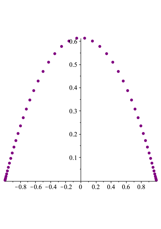
(a) Zeros of $p_{50}^{-i}(z)$.

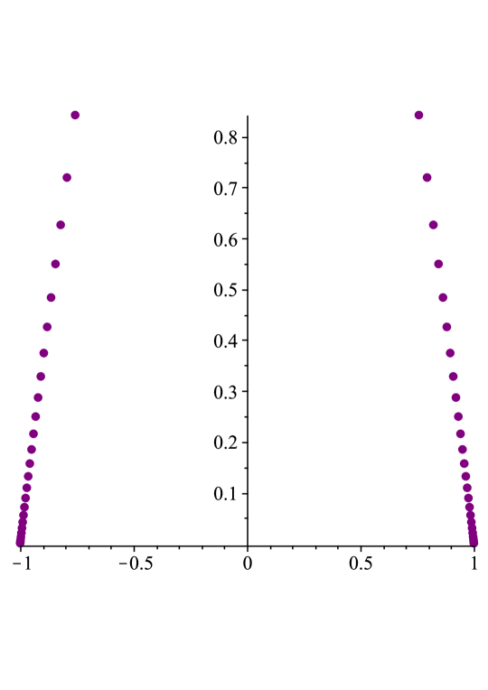
(b) Zeros of $p_{50}^{-2i}(z)$.

Figure 1. Zeros of $p_{50}^{-t}$ defined in (1.7) for $t=i<t_{c}$ and $t=2i>t_{c}$, where $t_{c}$ is the unique positive solution to (1.8).

(a) $s=-1-0.85i$.

(b) $s=-1-0.95i$.

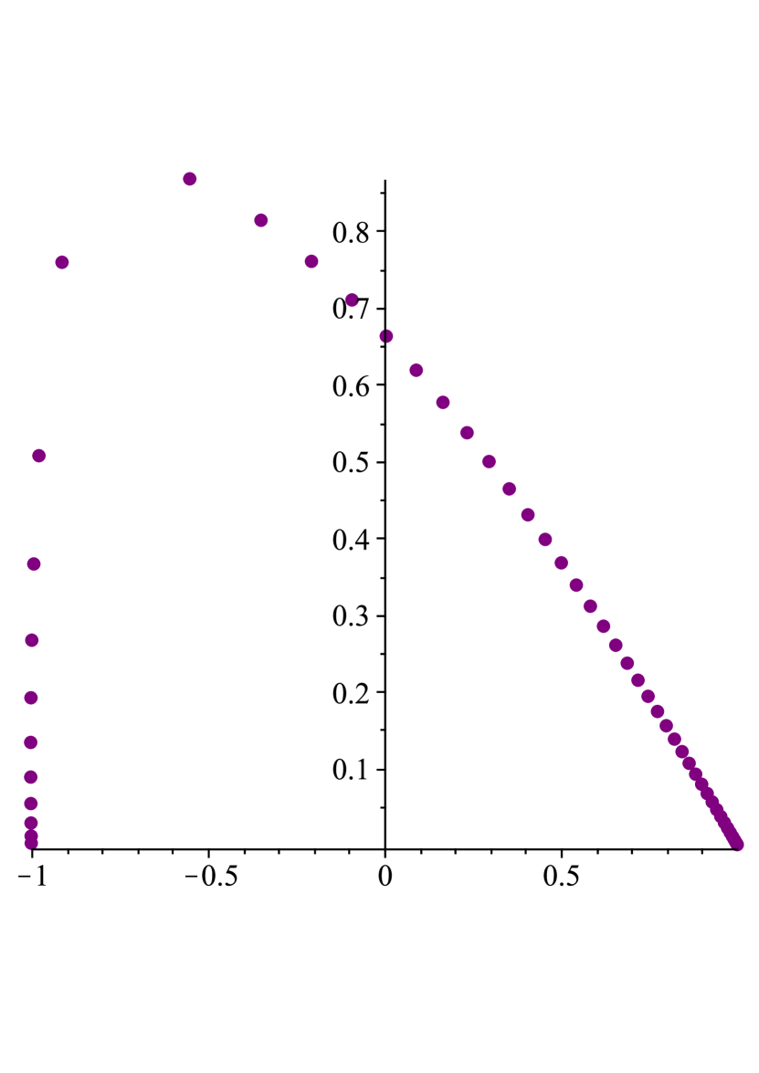
(c) $s=-1-1.05i$.

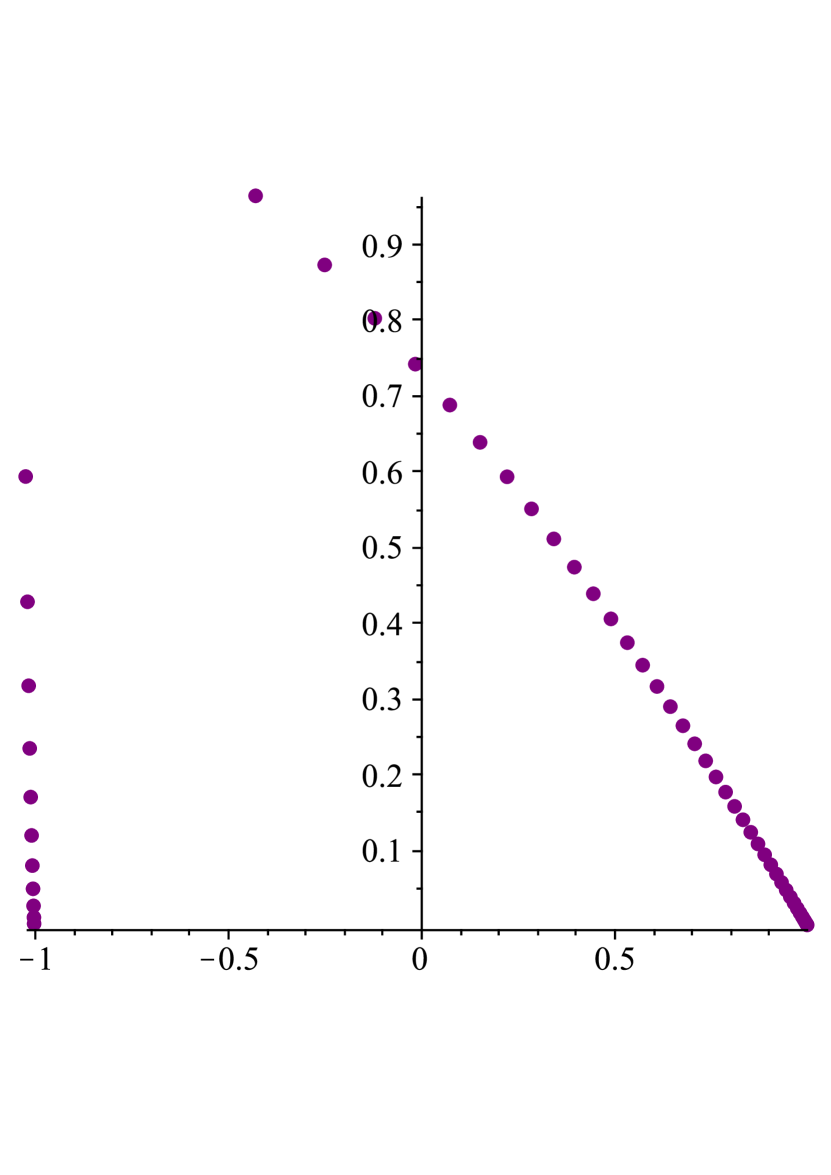
(d) $s=-1-1.15i$.

Figure 2. Zeros of $p_{50}(z;s)$ defined in (1.1) as $s$ moves from $s=-1-0.85i\in\mathfrak{G}_{0}$ to $s=-1-1.15i\in\mathfrak{G}_{1}^{-}$.

Despite many successful applications of potential theory to the analysis of non-Hermitian orthogonal polynomials via the GRS program, we adopt an alternate viewpoint based on deformation techniques born from advances in the theory of random matrices and integrable systems. We will make heavy use of the technique known as continuation in parameter space, first developed in the context of integrable systems (c.f. [44, 60, 61]), but which has only recently been applied in the field of orthogonal polynomials [13, 17, 18]. In contrast to the GRS program, where one constructs a so-called $g$-function as a solution to a certain variational problem, now one constructs a scalar function which solves a certain Riemann-Hilbert problem, which we call the $h$-function or modified external field.

We quickly note that as the weight function we consider, $\exp(-nf(z;s))$, depends on the parameter $s$, the scalar Riemann-Hilbert problem also depends on the parameter $s$. Importantly, the number of arcs over which this Riemann-Hilbert problem is posed, or equivalently the genus of the underlying Riemann surface, is also to be determined. Indeed, we will see that $h$-functions corresponding to Riemann surfaces of different genus lead to asymptotic expansions which possess markedly different behavior as $n\to\infty$. This difference is analogous to the difference in asymptotic behavior of the polynomials (and their recurrence coefficients) in the one cut and two cut cases, as described above for the GRS program. However, once one proves that for a specified genus and corresponding $s\in\mathbb{C}$ the scalar problem has a solution, one may continue with the process of steepest descent as will be outlined in Section 3 below.

We will see that the $h$-functions constructed in (1.10) and (1.15) are the desired $h$-functions corresponding to genus 0 and 1 regimes, respectively, when $s\in i\mathbb{R}_{-}$.

In order to establish the global phase portrait for all $s\in\mathbb{C}$, we deform these solutions off of the imaginary axis using the technique of continuation in parameter space discussed above. During this deformation process, we will encounter curves in the parameter space which separate regions of different genera. These curves in parameter space are called breaking curves and we denote the set of breaking curves, along with their endpoints, as $\mathfrak{B}$. For our purposes, breaking curves can only originate and terminate at what are called critical breaking points, and we will see that the only critical breaking points we encounter in the present work are $s=\pm 2$. The description of the breaking curves in the parameter space forms our first main result.

Theorem 2.1.

There are two critical breaking points at $s=\pm 2$ and $\mathfrak{B}=\mathfrak{b}_{-\infty}\cup\mathfrak{b}_{\infty}\cup\mathfrak{b}_{+}\cup\mathfrak{b}_{-}\cup\{\pm 2\}$. Here, $\mathfrak{b}_{-\infty}=\left(-\infty,-2\right)$ and $\mathfrak{b}_{\infty}=(2,\infty)$. The breaking curve $\mathfrak{b}_{+}$ connects $-2$ and $2$ while remaining in the upper half plane, and the breaking curve $\mathfrak{b}_{-}$ is obtained by reflecting $\mathfrak{b}_{+}$ about the real axis.

As seen in Figure 3, the set $\mathfrak{B}$ divides the parameter space into three connected components: $\mathfrak{G}_{0}$ and $\mathfrak{G}_{1}^{\pm}$.

Figure 3. Definitions of the regions $\mathfrak{G}_{0}$ and $\mathfrak{G}_{1}^{\pm}$ in the $s$-plane. The set $\mathfrak{B}$ is drawn in bold. The regular breaking points $\pm it_{c}$ are indicated on the breaking curves $\mathfrak{b}^{\pm}$, where we recall that $t_{c}$ was defined in (1.8).

We will see that the region $\mathfrak{G}_{0}$ corresponds to the genus $0$ region, whereas the regions $\mathfrak{G}_{1}^{\pm}$ correspond to genus $1$ regions.

Having determined the description of the set $\mathfrak{B}$, we will be able to deduce asymptotic formulas for the recurrence coefficients for the orthogonal polynomials defined in (1.1) for all $s\in\mathbb{C}\setminus\mathfrak{B}$ via deformation techniques. We quickly digress to discuss notation before stating these results. We first introduce monic polynomials, $p_{n}^{N}(z;s)$ which satisfy the following orthogonality conditions.

$$\int_{-1}^{1}p_{n}^{N}(z;s)z^{k}e^{-Nf(z;s)}\,dz=0,\qquad k=0,1,\dots,n-1,$$ (2.1)

where $N$ is a fixed integer. Note that for each $N\in\mathbb{N}$, we have a family of polynomials $\{p_{n}^{N}(z;s)\}_{n=0}^{\infty}$. The polynomials that we consider in (1.1) are given by $p_{n}(z;s)=p_{n}^{n}(z;s)$; that is, we consider the polynomials along the diagonal where $N=n$. Now, provided the polynomials exist for the appropriate values for $n,N$, and $s$, they satisfy the following three term recurrence relation

$$zp_{n}^{N}(z;s)=p_{n+1}^{N}(z;s)+\alpha_{n}^{N}(s)p_{n}^{N}(z;s)+\beta_{n}^{N}(s)p_{n-1}^{N}(z;s).$$ (2.2)

In the present work, we concern ourselves with the situation $N=n$, and for sake of notation we set $\alpha_{n}:=\alpha_{n}^{n}$ and $\beta_{n}:=\beta_{n}^{n}$. It should be stressed that the polynomials $p_{n-1}$, $p_{n}$ and $p_{n+1}$ do not satisfy the recurrence relation (2.2). We now state our second result, on the asymptotics of the recurrence coefficients in the region $\mathfrak{G}_{0}$.

Theorem 2.2.

Let $s\in\mathfrak{G}_{0}$. Then the recurrence coefficients $\alpha_{n}$ and $\beta_{n}$ exist for large enough $n$, and they satisfy, as $n\to\infty$,

$$\alpha_{n}(s)=\frac{2s}{(s^{2}-4)^{2}}\frac{1}{n^{2}}+\mathcal{O}\left(\frac{1}{n^{3}}\right),\qquad\beta_{n}(s)=\frac{1}{4}+\frac{s^{2}+4}{4(s^{2}-4)^{2}}\frac{1}{n^{2}}+\mathcal{O}\left(\frac{1}{n^{4}}\right).$$ (2.3)

As mentioned above, for $s\in\mathfrak{G}_{1}^{\pm}$, the underlying Riemann surface has genus $1$. Indeed, the Riemann surface corresponds to the algebraic equation $\xi^{2}=Q(z;s)$, where $Q$ is a rational function, and we take the branch cuts for the Riemann surface on two arcs - one connecting $1$ to $\lambda_{0}(s)$, labeled $\gamma_{m,0}$, and the other connecting $-1$ to $\lambda_{1}(s)$, labeled $\gamma_{m,1}$, where $\lambda_{0}$ and $\lambda_{1}$ will be determined. Moreover, for $s\in\mathfrak{G}_{1}^{\pm}$, the asymptotics of the recurrence coefficients will depend on theta functions on our Riemann surface. These theta functions will be used to construct functions $\mathcal{M}_{1}(z,k)$ and $\mathcal{M}_{2}(z,k)$, along with a constant $d$, whose precise descriptions we provide in Section 3.6. The functions $\mathcal{M}_{1,n}(z,d)\equiv\mathcal{M}_{1}(z,d)$ and $\mathcal{M}_{2,n}(z,d)\equiv\mathcal{M}_{2}(z,d)$ are holomorphic in $\mathbb{C}\setminus(\gamma_{m,0}\cup\gamma_{m,1}\cup\gamma_{c,1})$, where $\gamma_{c,1}$ is a to be determined curve connecting $\lambda_{0}(s)$ to $\lambda_{1}(s)$, and have at most one simple zero there. Furthermore, for $N=n$ and given $\epsilon>0$, we will need to consider asymptotic results on a subsequence $\mathbb{N}(s,\epsilon)$, whose precise definition we defer to Section 3.6. However, to make use of this subsequence, we need to know that the cardinality of the set $\mathbb{N}(s,\epsilon)$ is infinite, which we prove in Lemma 3.2. These functions $\mathcal{M}_{1,n}(z,d)$ and $\mathcal{M}_{2,n}(z,d)$ arise in the asymptotics of the recurrence coefficients for $s\in\mathfrak{G}_{1}^{\pm}$, which we state below.

Theorem 2.3.

Let $s\in\mathfrak{G}_{1}^{\pm}$ and $n\in\mathbb{N}(s,\epsilon)$. Then the recurrence coefficients $\alpha_{n}$ and $\beta_{n}$ exist for large enough $n$, and they satisfy, as $n\to\infty$,

$$\alpha_{n}(s)=\frac{\lambda_{1}^{2}(s)-\lambda_{0}^{2}(s)}{4+2\lambda_{0}(s)-2\lambda_{1}(s)}+\frac{d}{dz}\left[\log\mathcal{M}_{2,n}(1/z,d)-\log\mathcal{M}_{2,n}(1/z,-d)\right]\Big{|}_{z=0}+\mathcal{O}_{\epsilon}\left(\frac{1}{n}\right)$$ (2.4)

and

$$\beta_{n}(s)=\frac{(2+\lambda_{0}(s)-\lambda_{1}(s))^{2}}{16}\frac{\mathcal{M}_{1,n}(\infty,-d)\mathcal{M}_{2,n}(\infty,d)}{\mathcal{M}_{1,n}(\infty,d)\mathcal{M}_{2,n}(\infty,-d)}+\mathcal{O}_{\epsilon}\left(\frac{1}{n}\right),$$ (2.5)

Above, the notation $f(n)=\mathcal{O}_{\epsilon}(1/n)$ indicates that there exists a constant which depends only on $\epsilon$, $M=M(\epsilon)$, such that $\left|f(n)\right|\leq M/n$ for large enough $n$. We recall that the parameter $\epsilon$ is used to define the set of valid indices, $\mathbb{N}(s,\epsilon)$, along which we take limits. Having determined the asymptotics of the recurrence coefficients of the polynomials in (1.1) when $s\in\mathbb{C}\setminus\mathfrak{B}$, our final two results recover these asymptotics when $s\in\mathfrak{B}$.

As seen in Theorem 2.1, the breaking curves $\mathfrak{b}_{-\infty}$ and $\mathfrak{b}_{\infty}$ are the intervals $(-\infty,-2)$ and $(2,\infty)$, respectively. The theory of orthogonal polynomials with respect to real weights, varying or otherwise, has been written about extensively in the literature, most notably from the viewpoint of potential theory. In particular, the results of Deift, Kriecherbauer, and McLaughlin in [30] can be applied in conjunction with the GRS program to show that the empirical zero counting measure of the polynomials in (1.1) converge to a continuous measure supported on the interval $[-1,1]$ as $n\to\infty$, when $s\in\mathbb{R}$ and $|s|<2$. The results of [30] can also be used to show that the corresponding limit measure is supported on $[-1,a)$ for some $a<1$ when $s>2$. Similarly, one also has that this measure is supported on $(b,1]$ for some $b>-1$ when $s\in\mathbb{R}$ is such that $s<-2$. The difference in the support of the limiting measure when $|s|>2$ and $|s|<2$ is also of interest in random matrix theory, and occurs when the soft edge meets the hard edge (see the work of Claeys and Kuijlaars [26]). The asymptotics of orthogonal polynomials corresponding to the case $s\in\mathfrak{b}_{\infty}\cup\mathfrak{b}_{-\infty}$ follow from [5, Theorem 2]. From the viewpoint of the present work, the transitions at $s=\pm 2$ can be seen to come from the fact these are critical breaking points.

As the case where $s\in\mathbb{R}\cap\mathfrak{B}$ has been extensively studied, we next consider the asymptotic behavior of the recurrence coefficients as we approach a regular breaking point which is not on the real line. More precisely, we let $s_{*}$ be a regular breaking point in $\mathfrak{b}_{+}\cup\mathfrak{b}_{-}$ and we let $s$ approach $s_{*}$ as

$$s=s_{*}+\frac{L_{1}}{n},$$ (2.6)

where $L_{1}\in\mathbb{C}$ is such that $s=s(n)\in\mathfrak{G}_{0}$ for large enough $n$. The scaling limit (2.6) is referred to as the double scaling limit, as it describes the behavior of the polynomials as both $n\to\infty$ and $s\to s_{*}$. This formulation then leads to the following description of the recurrence coefficients in the aforementioned double scaling limit.

Theorem 2.4.

Let $s^{*}\in\mathfrak{b}_{+}\cup\mathfrak{b}_{-}$ and let $s\to s_{*}$ as described in (2.6). Then the recurrence coefficients exist for large enough $n$, and they satisfy

$$\alpha_{n}(s)=\frac{\delta_{n}\left(2-\sqrt{4-s^{2}_{*}}\right)\sqrt{4-s_{*}^{2}}}{\sqrt{\pi}s_{*}^{3}n^{1/2}}\frac{1}{n^{1/2}}-\frac{2\delta_{n}^{2}\left(2-\sqrt{4-s_{*}^{2}}\right)^{2}}{\pi s_{*}^{5}}\frac{1}{n}+\mathcal{O}\left(\frac{1}{n^{3/2}}\right)$$ (2.7a)

and

$$\beta_{n}(s)=\frac{1}{4}+\frac{\sqrt{4-s_{*}^{2}}}{2\sqrt{\pi}s_{*}^{2}}\frac{1}{n^{1/2}}-\frac{\delta_{n}^{2}}{2\pi s_{*}^{2}}\frac{1}{n}+\mathcal{O}\left(\frac{1}{n^{3/2}}\right),$$ (2.7b)

as $n\to\infty$, where

$$\delta_{n}=\delta_{n}(L_{1})=e^{-in\kappa}\exp\left(L_{1}\left(\frac{4}{s_{*}^{2}}-1\right)^{1/2}\right),\qquad\kappa\in\mathbb{R},$$ (2.8)

and $\kappa$ is a constant given in (5.49).

Note above that

$$\left|\delta_{n}\right|=\exp\left(\Re\left[L_{1}\left(\frac{4}{s_{*}^{2}}-1\right)^{1/2}\right]\right),$$ (2.9)

as $\kappa\in\mathbb{R}$ and that the recurrence coefficients decay at a rate of $n^{1/2}$. In particular, the modulus of $\delta_{n}$ does not depend on $n$.

Now, we are just left with investigating the behavior of the recurrence coefficients for $s$ near the critical breaking points $s=\pm 2$. For brevity, we focus just on the case $s=2$, although we note that the case $s=-2$ can be handled similarly via reflection, as $\exp(-nf(z;-s))=\exp(-nf(-z;s))$. To state our results, we consider the Painlevé II equation [53, Chapter 32]:

$$q^{\prime\prime}(x)=xq(x)+2q^{3}(x)-\alpha,\qquad\alpha\in\mathbb{C}.$$ (2.10)

Next, let $q=q(w)$ be the generalized Hastings-McLeod solution to Painlevé II with the parameter $\alpha=1/2$, which is characterized by the following asymptotic behavior

$$q(x)=\begin{cases}\displaystyle\sqrt{-\frac{x}{2}}+\mathcal{O}\left(\frac{1}{x}\right),\qquad&x\to-\infty\\[5.69054pt] \displaystyle\frac{1}{2x}+\mathcal{O}\left(\frac{1}{x^{4}}\right)&x\to\infty.\end{cases}$$ (2.11)

In order to study the asymptotics of the recurrence coefficients as $s\to 2$, we take $s$ in a double scaling regime near this critical point as

$$s=2+\frac{L_{2}}{n^{2/3}},$$ (2.12)

where we impose that $L_{2}<0$. This leads us to our final main finding.

Theorem 2.5.

Let $s\to 2$ as described in (2.12). Then the recurrence coefficients exist for large enough $n$, and they satisfy

$$\alpha_{n}(s)=-\frac{q^{2}(-L_{2})+q^{\prime}(-L_{2})}{n^{2/3}}+\mathcal{O}\left(\frac{1}{n}\right),\qquad\beta_{n}(s)=\frac{1}{4}-\frac{q^{2}(-L_{2})+q^{\prime}(-L_{2})}{2}\frac{1}{n^{2/3}}+\mathcal{O}\left(\frac{1}{n}\right),$$ (2.13)

as $n\to\infty$, where $q$ is the generalized Hastings-McLeod solution to Painlevé II with parameter $\alpha=1/2$. Furthermore, the function $U(w)=q^{2}(w)+q^{\prime}(w)$ is free of poles for $w\in\mathbb{R}$.

Plots of the recurrence coefficients are given in Figures 4 and 5, and should be compared with Theorems 2.2 and 2.5.

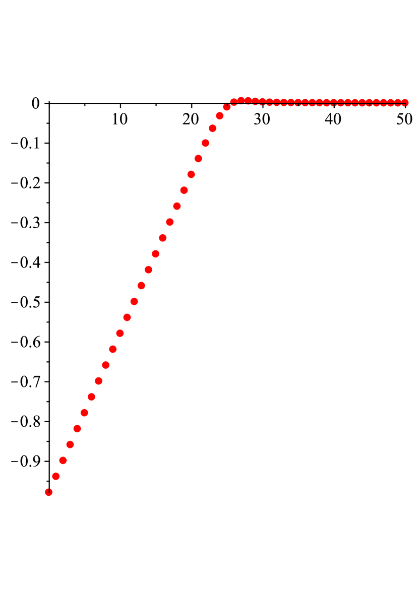
(a) $\alpha_{n}(1)$.

(b) $\alpha_{n}(2)$.

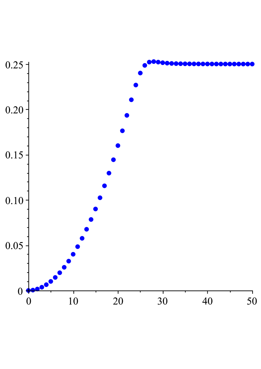
(c) $\beta_{n}(1)$.

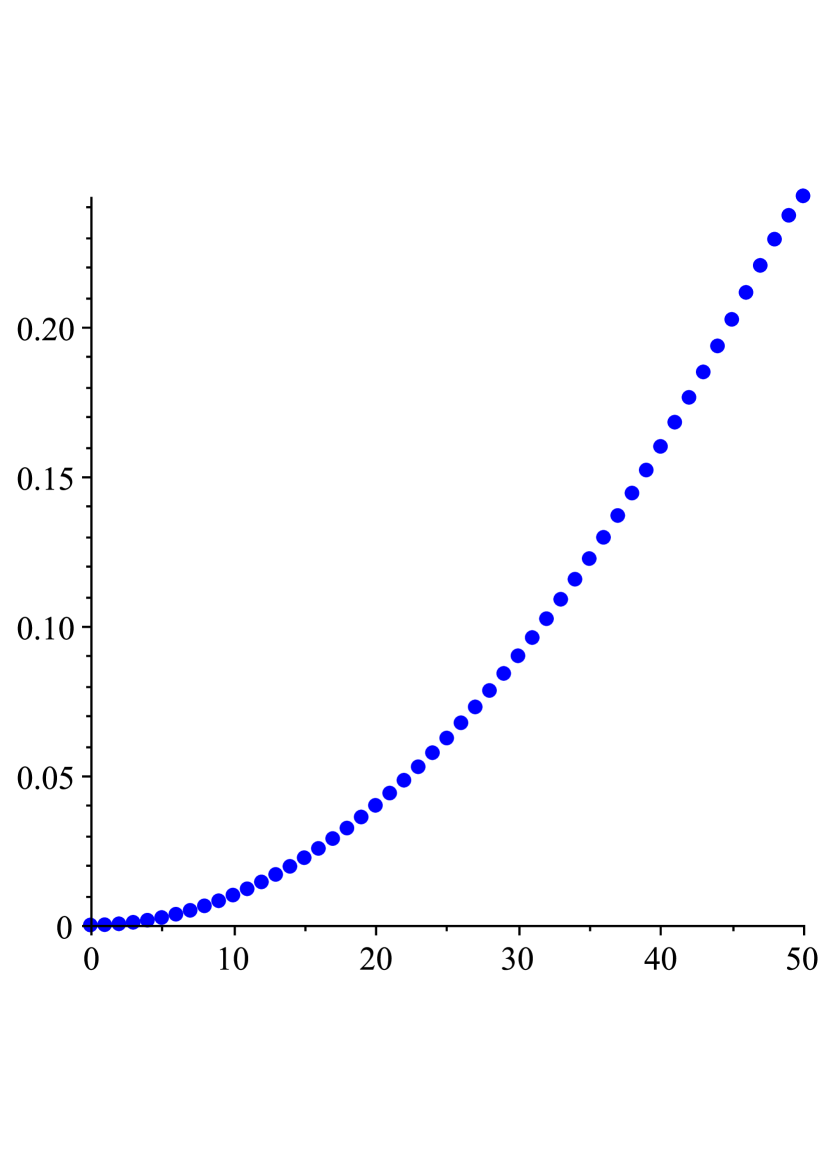
(d) $\beta_{n}(2)$.

Figure 4. Plots of $\alpha_{n}(s)$ and $\beta_{n}(s)$ for $n=0,\dots,50$, with $s=1,2$.

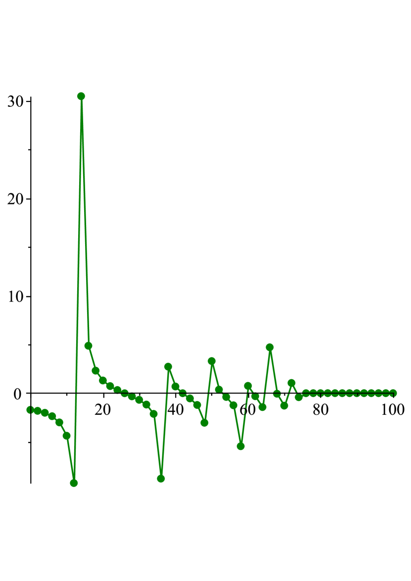
(a) $\Im\alpha_{2n}(i)$.

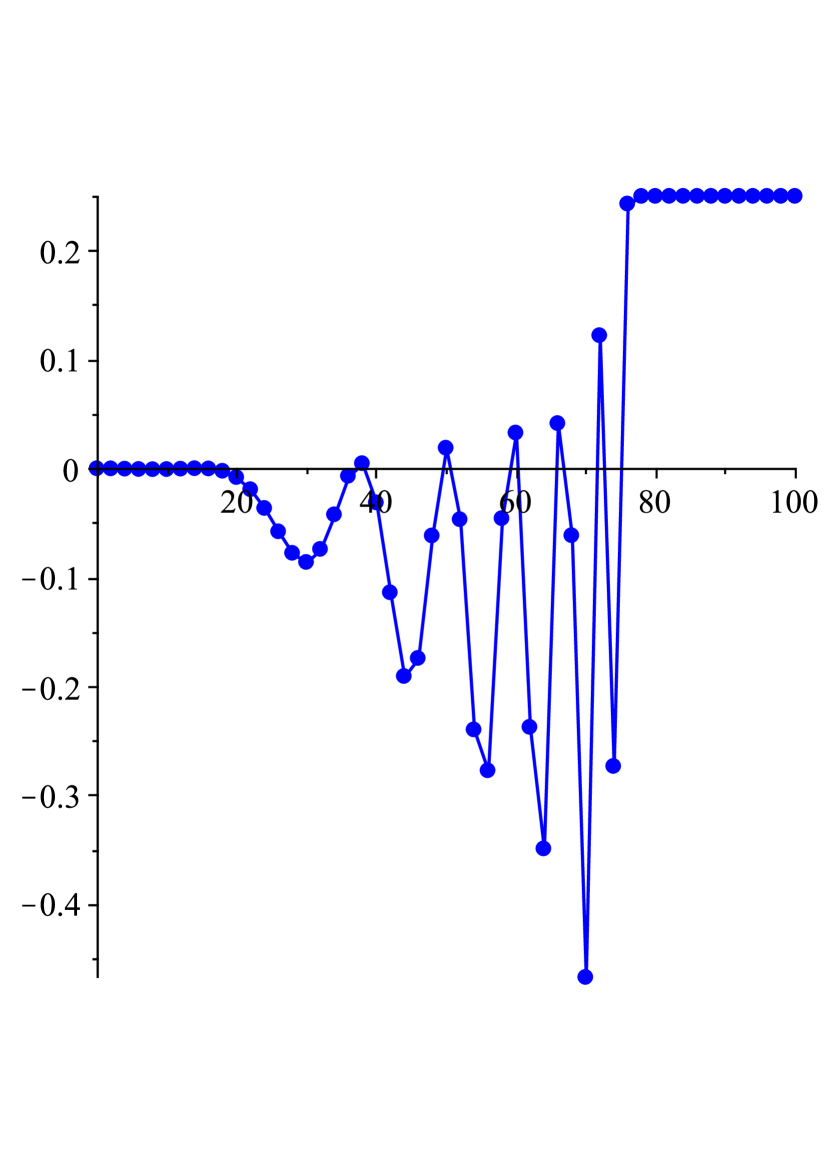
(b) $\Re\beta_{2n}(i)$.

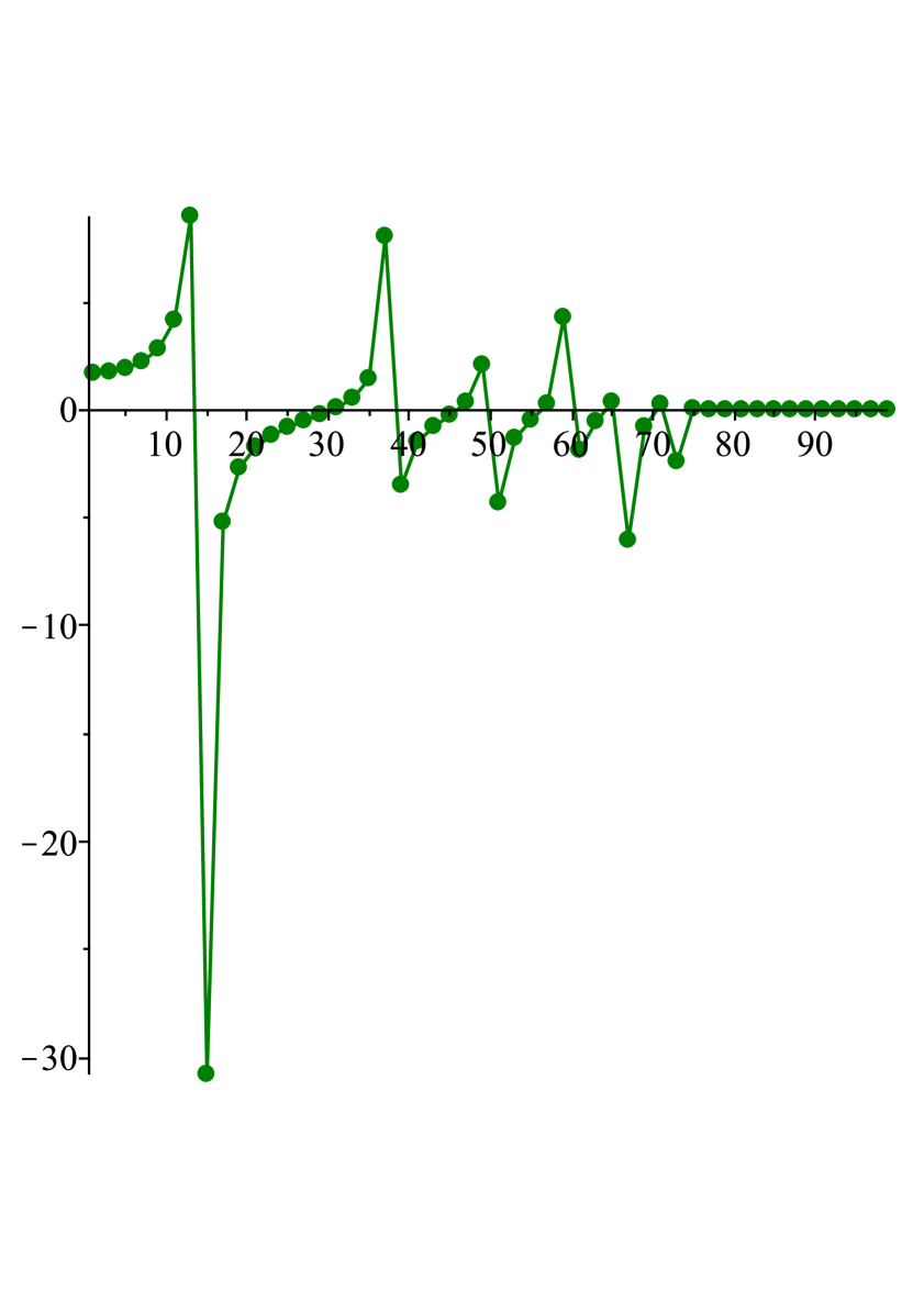
(c) $\Im\alpha_{2n+1}(i)$.

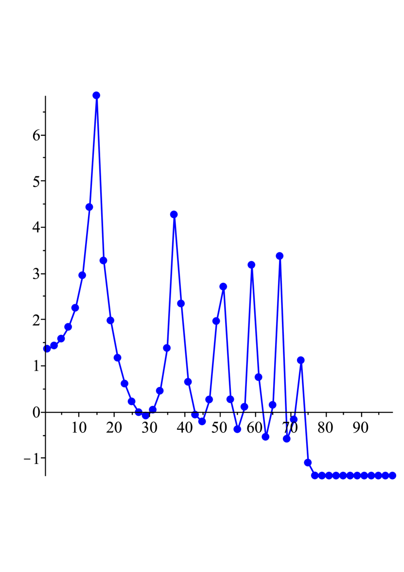
(d) $\log\Re\beta_{2n+1}(i)$.

Figure 5. Plots of $\Im\alpha_{n}(s)$ and $\Re\beta_{n}(s)$ for $n=0,\dots,100$, with $s=i$.

Figures 1, 2, 4, and 5 have been computed using the nonlinear discrete string equations for the recurrence coefficients presented in [12, Theorem 2, Theorem 4], see also [62, §5.2]. In Figure 5, we have used from [23] that $\beta_{n}(s)\in\mathbb{R}$ and $\alpha_{n}(s)\in i\mathbb{R}$ when $s\in i\mathbb{R}$. Moreover, it was also shown in [23] that for fixed $n$, $\alpha_{n}(t)$ and $\beta_{2n+1}(it)$ will have poles (as a function of $t$) for $t\in\mathbb{R}$. As such, we have plotted $\Re\beta_{2n+1}$ on a log scale in Figure 5(d). Once the recurrence coefficients $\alpha_{n}(s)$ and $\beta_{n}(s)$ have been computed, we assemble the Jacobi matrix for the orthogonal polynomials and calculate its eigenvalues, which correspond to the zeros of $p_{50}(z;s)$, as explained for instance in [25, 37]. Calculations have been done in Maple, using an extended precision of 100 digits.

Overview of Paper

The outline of the present paper is as follows. In Section 3, we provide a review on the Riemann-Hilbert problem for the orthogonal polynomials and the method of nonlinear steepest descent pioneered by Deift and Zhou in the early 1990s. In particular, we show how the existence of a suitable $h$-function can be used to obtain strong asymptotics of the polynomials throughout the complex plane and asymptotics of the recurrence coefficients. Moreover, we also prove Lemma 3.2 when discussing solutions to the global parametrix in Section 3.6.

In Section 4, we implement the technique of continuation in parameter space to obtain the desired $h$-function for $s\in\mathbb{C}\setminus\mathfrak{B}$. In this section, we prove Theorems 2.1, 2.2, and 2.3.

In Section 5, we study the double scaling limit as $s\to s_{*}$, where $s^{*}\in\mathfrak{b}_{+}\cup\mathfrak{b}_{-}$. Moreover, we prove Theorem 2.4 in the final part of this section.

Finally, in Section 6, we complete our analysis by investigating the double scaling limit as $s\to 2$ via (2.12). We end the paper with a proof of Theorem 2.5.

Acknowledgments

The authors would like to thank Arieh Iserles, Guilherme Silva, and Maxim Yattselev for their guidance and discussions on all aspects of the Kissing polynomials and the Riemann-Hilbert approach to these polynomials. This work was carried out while A.F.C. was a PhD student at the University of Cambridge, and he is thankful for his current support by the Cantab Capital Institute for the Mathematics of Information and the Cambridge Centre for Analysis. A. D. gratefully acknowledges financial support from EPSRC, grant EP/P026532/1, Painlevé equations: analytical properties and numerical computation.

3. The Riemann-Hilbert Problem and Overview of Steepest Descent

The formulation of the orthogonal polynomials as a solution to a Riemann-Hilbert problem was first given by Fokas, Its, and Kitaev in the early 1990s [36]. This formulation became even more powerful in the late 1990s due to the development of the nonlinear steepest descent method to obtain asymptotic solutions to Riemann-Hilbert problems, developed by Deift and Zhou [31, 32, 33]. In this section, we review the Riemann-Hilbert problem and nonlinear steepest descent as it relates to the polynomials defined in (1.1). We refer the reader to the works [19, 29] for more details on these issues.

3.1. The Riemann-Hilbert Problem and The Modified External Field

Given a smooth curve $\Sigma$ connecting $-1$ to $1$ in $\mathbb{C}$, oriented from $-1$ to $1$, consider the following Riemann-Hilbert problem for $Y:\mathbb{C}\setminus\Sigma\to\mathbb{C}^{2\times 2}$,

$$Y_{n}^{N}(z;s)\text{ is analytic for }z\in\mathbb{C}\setminus\Sigma,\qquad$$ (3.1a)

$$Y_{n,+}^{N}(z;s)=Y_{n,-}^{N}(z;s)\begin{pmatrix}1&e^{-Nf(z;s)}\\ 0&1\end{pmatrix},\qquad z\in\Sigma,$$ (3.1b)

$$Y_{n}^{N}(z;s)=\left(I+\mathcal{O}\left(\frac{1}{z}\right)\right)z^{n\sigma_{3}},\qquad z\to\infty,$$ (3.1c)

$$Y_{n}^{N}(z;s)=\mathcal{O}\begin{pmatrix}1&\log\left|z\mp 1\right|\\ 1&\log\left|z\mp 1\right|\end{pmatrix},\qquad z\to\pm 1.$$ (3.1d)

Above, $\sigma_{3}$ is the Pauli matrix given by $\sigma_{3}=\operatorname{diag}(1,-1)$. For notational convenience, we drop the dependence of the above RHP and its solution on $s$ and $n$. We also define $\kappa_{n,N}$ as the normalizing constant for $p_{n}^{N}$, obtained via

$$\int_{-1}^{1}(p_{n}^{N}(z;s))^{2}e^{-Nf(z;s)}dz=\frac{1}{\kappa_{n,N}^{2}}.$$ (3.2)

The existence of $Y$ is equivalent to the existence of the monic orthogonal polynomial $p_{n}^{N}$ defined in (2.1), of degree exactly $n$, and, furthermore, if $\kappa_{n-1,N}$ is finite and non-zero, then $Y$ is explicitly given by

$$Y(z)=\begin{pmatrix}p_{n}^{N}(z)&\left(\mathcal{C}p_{n}^{N}e^{-Nf}\right)(z)\\ -2\pi i\kappa_{n-1,N}^{2}p_{n-1}^{N}(z)&-2\pi i\kappa_{n-1,N}^{2}\left(\mathcal{C}p_{n-1}^{N}e^{-Nf}\right)(z)\end{pmatrix}.$$ (3.3)

We recall that throughout the present analysis we take $N=n$, and we also drop the dependence of $Y$ on $N$ for notational convenience. In (3.3), $\mathcal{C}g$ denotes the Cauchy transform of the function $g$ along $\Sigma$, i.e.

$$\left(\mathcal{C}g\right)(z)=\frac{1}{2\pi i}\int_{\Sigma}\frac{g(u)}{u-z}\,du,$$

which is analytic in $\mathbb{C}\setminus\Sigma$. The Deift-Zhou method of nonlinear steepest descent is a powerful method of determining large $n$ asymptotics of solutions to these types of Riemann-Hilbert problems, and as such, we can use it to determine asymptotics of the polynomials $p_{n}$ and related quantities.

The first transformation requires the existence of a modified external field, or h-function, whose properties we describe below. First, we define $\gamma_{c,0}:=(-\infty,-1]$ and set $\Omega=\Omega(s)=\gamma_{c,0}\cup\Sigma$. Next we partition $\Omega$ into two subsets as $\Omega=\mathfrak{M}\cup\mathfrak{C}$, where the arcs in $\mathfrak{M}$ are denoted main arcs and those in $\mathfrak{C}$ are denoted complementary arcs. Once this partitioning has been completed, we may define a hyperelliptic Riemann surface $\mathfrak{R}=\mathfrak{R}(s)$ whose branchcuts are precisely the main arcs in $\mathfrak{M}$ and whose branchpoints we define to be the set $\Lambda=\Lambda(s)$ . If the genus of $\mathfrak{R}$ is $L$, we may write $\mathfrak{M}=\cup_{j=0}^{L}\gamma_{m,j}$ and $\mathfrak{C}=\cup_{j=0}^{L}\gamma_{c,j}$. Moreover, when we refer to the genus of $h$, we are referring to the genus of the associated Riemann surface. Finally, we impose that all arcs in $\Omega$ are bounded, aside from the one complementary arc $\gamma_{c,0}$.

The question remains: how do we partition $\Sigma$ and choose the arcs in $\mathfrak{M}$ and $\mathfrak{C}$? Equivalently, we may ask: how do we choose the appropriate genus $L$? In order to make the appropriate first transformation to (3.1) to begin the process of steepest descent, we must first construct a function $h$ that satisfies both a scalar Riemann-Hilbert problem on $\Omega$ and certain inequalities, to be described below. Therefore, the arcs in $\mathfrak{M}$ and $\mathfrak{C}$, and also the genus $L$, are chosen so that we can construct a suitable $h$-function. The modified external field must satisfy:

$$h(z;s)\text{ is analytic for }z\in\mathbb{C}\setminus\Omega,\qquad$$ (3.4a)

$$h_{+}(z;s)-h_{-}(z;s)=4\pi i\eta_{j},\qquad z\in\gamma_{c,j},$$ (3.4b)

$$h_{+}(z;s)+h_{-}(z;s)=4\pi i\omega_{j},\qquad z\in\gamma_{m,j},$$ (3.4c)

$$h(z;s)=-f(z;s)-\ell+2\log z+\mathcal{O}\left(\frac{1}{z}\right),\qquad z\to\infty$$ (3.4d)

$$\Re h(z;s)=\mathcal{O}\left((z\mp 1)^{1/2}\right),\qquad z\to\pm 1,$$ (3.4e)

$$\Re h(z;s)=\mathcal{O}\left((z-\lambda)^{3/2}\right),\qquad z\to\lambda,\quad\lambda\in\Lambda\setminus\{\pm 1\},$$ (3.4f)

for $j=0,1,\dots,L$. Above, we impose that $\omega_{L}=0$ and $\eta_{0}=1$; the remaining real constants $\eta_{j}$ and $\omega_{j}$ (which only depend on $s$) can be chosen arbitrarily to satisfy (3.4). Furthermore, the constant $\ell=\ell(s)$ depends only on the parameter $s$.

Remark 3.1.

Given any genus $L$ and arbitrary constants $\ell,\eta_{j},\omega_{j}\in\mathbb{R}$, there is no guarantee that a solution to (3.4) even exists. However, if such a solution does exist, it will be unique.

Remark 3.2.

Assuming that $L=0$ or $L=1$ and provided we are able to construct a solution to (3.4), we define the Riemann surface $\mathfrak{R}$ to be the two-sheeted genus $L$ Riemann surface associated to the algebraic equation

$$\xi^{2}=h^{\prime}(z)^{2}=\Pi^{2}(z)R(z),$$ (3.5)

where

$$R(z)=\frac{1}{z^{2}-1}\prod_{j=0}^{2L-1}(z-\lambda_{j}),$$ (3.6)

and $\Pi(z)$ is a polynomial of degree $1-L$, chosen so that $h^{\prime}$ possess the correct asymptotics at infinity. The branch cuts of $\mathfrak{R}$ are taken along $\gamma_{m,j}$, $j=0,\dots,L$, and the top sheet is fixed so that

$$\xi(z)=-f^{\prime}(z;s)+\mathcal{O}\left(\frac{1}{z}\right)=-s+\mathcal{O}\left(\frac{1}{z}\right),\qquad z\to\infty_{1}.$$ (3.7)

In addition to solving the above scalar Riemann-Hilbert problem, $h$ must also satisfy the following inequalities

$$\Re h(z)<0\text{ if }z\text{ is an interior point of any bounded complementary arc }\gamma_{c}\in\mathfrak{C},$$ (3.8a)

$$\Re h(z_{0})>0\text{ for }z_{0}\text{ in close proximity to any interior point of a main arc }\gamma_{m}\in\mathfrak{M}.$$ (3.8b)

If $s\in\mathbb{C}$ is such that we can construct a function $h(z;s)$ satisfying both (3.4) and (3.8), we call $s$ a regular point. Now, provided $s$ is a regular point, we may proceed with the process of nonlinear steepest descent as follows.

3.2. Overview of Deift-Zhou Nonlinear Steepest Descent

The first transformation of steepest descent aims to normalize the Riemann-Hilbert problem at infinity. To do so, we define

$$T(z):=e^{-n\ell\sigma_{3}/2}Y(z)e^{-\frac{n}{2}\left[h(z)+f(z)\right]\sigma_{3}},$$ (3.9)

where we recall that $\ell\in\mathbb{R}$ is defined by (3.4d) and $f(z;s)=sz$. By making this transformation, we see that $T$ satisfies the following Riemann-Hilbert problem:

$$T(z)\text{ is analytic for }z\in\mathbb{C}\setminus\Sigma,\qquad$$ (3.10a)

$$T_{+}(z)=T_{-}(z)\begin{pmatrix}e^{-\frac{n}{2}\left(h_{+}(z)-h_{-}(z)\right)}&e^{\frac{n}{2}\left(h_{+}(z)+h_{-}(z)\right)}\\ 0&e^{\frac{n}{2}\left(h_{+}(z)-h_{-}(z)\right)}\end{pmatrix},\qquad z\in\Sigma,$$ (3.10b)

$$T(z)=I+\mathcal{O}\left(\frac{1}{z}\right),\qquad z\to\infty,$$ (3.10c)

$$T(z)=\mathcal{O}\begin{pmatrix}1&\log\left|z\mp 1\right|\\ 1&\log\left|z\mp 1\right|\end{pmatrix},\qquad z\to\pm 1.$$ (3.10d)

Note that the Riemann-Hilbert problem above also depends on $s$, but we have again dropped this dependence for notational convenience. We also remark that (3.4c) and (3.8b) imply that $\Re h(z)=0$ for $z\in\mathfrak{M}$. As $\mathfrak{M}$ is part of the zero level set of $\Re h$, the jump matrix for $T$ has highly oscillatory diagonal entries when $z\in\mathfrak{M}$. Furthermore, if $z\in\mathfrak{C}\setminus\gamma_{c,0}$, the diagonal entries of the jump matrix will be constant and purely imaginary. Moreover, the $(1,2)$-entry of the jump matrix will decay exponentially quickly to $0$ by (3.8a). The next transformation of the steepest descent process deforms the jump contours so that the highly oscillatory entries of the jump matrix decay exponentially quickly, and is referred to as the opening of lenses.

The opening of lenses relies on the following factorization of the jump matrix across a main arc

$$\begin{pmatrix}e^{-nH(z)}&e^{2\pi in\omega_{j}}\\ 0&e^{nH(z)}\end{pmatrix}=\begin{pmatrix}1&0\\ e^{n\left(H(z)-2\pi i\omega_{j}\right)}&1\end{pmatrix}\begin{pmatrix}0&e^{2\pi in\omega_{j}}\\ -e^{-2\pi in\omega_{j}}&0\end{pmatrix}\begin{pmatrix}1&0\\ e^{n\left(-H(z)-2\pi i\omega_{j}\right)}&1\end{pmatrix},$$ (3.11)

where we have defined $H(z)=\left(h_{+}(z)-h_{-}(z)\right)/2$. On the $+$-side ($-$-side) of each main arc, we define $\gamma_{m,j}^{+}$ ($\gamma_{m,j}^{-}$) to be an arc which starts and ends at the endpoints of $\gamma_{m,j}$ and remains entirely on the $+$($-$) side of $\gamma_{m,j}$. For now we do not impose any restrictions on the precise description of these arcs, but we enforce that they remain in the region where $\Re h>0$, which is possible due to (3.8b). We define $\mathcal{L}_{j}^{\pm}$ to be the region bounded between the arcs $\gamma_{m,j}$ and $\gamma_{m,j}^{\pm}$, respectively, and set $\hat{\Sigma}:=\Sigma\cup_{j=0}^{L}\left(\gamma_{m,j}^{+}\cup\gamma_{m,j}^{-}\right)$ as in Figure 6.

Figure 6. The contour $\hat{\Sigma}$ after opening lenses in the case $L=1$.

We can now define the third transformation of the steepest descent process as

$$S(z):=\begin{cases}T(z)\begin{pmatrix}1&0\\ \mp e^{-nh(z)}&1\end{pmatrix},\qquad&z\in\mathcal{L}_{j}^{\pm},\\ T(z),\qquad&\text{otherwise}.\end{cases}$$ (3.12)

We then have that $S$ solves the following Riemann-Hilbert problem on $\hat{\Sigma}$:

$$S(z)\text{ is analytic for }z\in\mathbb{C}\setminus\hat{\Sigma},\qquad$$ (3.13a)

$$S_{+}(z)=S_{-}(z)j_{S}(z),\qquad z\in\hat{\Sigma},$$ (3.13b)

$$S(z)=I+\mathcal{O}\left(\frac{1}{z}\right),\qquad z\to\infty,$$ (3.13c)

Note that for $z\in\gamma_{m,j}^{\pm}$,

$$j_{S}(z)=\begin{pmatrix}1&0\\ e^{-nh(z)}&1\end{pmatrix},$$ (3.14)

which decays exponentially quickly to the identity as $n\to\infty$, due to (3.8b). As $S=T$ outside of the lenses, we see that there are no changes to the jump matrix across a complementary arc, so that

$$j_{S}(z)=\begin{pmatrix}e^{-2\pi in\eta_{j}}&e^{\frac{n}{2}(h_{+}(z)+h_{-}(z))}\\ 0&e^{2\pi in\eta_{j}}\end{pmatrix},\qquad z\in\gamma_{c,j},$$ (3.15)

which again tends exponentially quickly to a diagonal matrix as $n\to\infty$. Finally, we see that over $\gamma_{m,j}$, the jump matrix is given by

$$j_{S}(z)=\begin{pmatrix}0&e^{2\pi in\omega_{j}}\\ -e^{-2\pi in\omega_{j}}&0\end{pmatrix},\qquad z\in\gamma_{m,j},$$ (3.16)

which follows from the factorization (3.11). Now consider the following model Riemann-Hilbert problem for the global parametrix, $M$, which is obtained by neglecting those entries in the jump matrices which are exponentially close to the identity in the Riemann-Hilbert problem for $S$,

$$M(z)\text{ is analytic for }z\in\mathbb{C}\setminus\Sigma,\qquad$$ (3.17a)

$$M_{+}(z)=M_{-}(z)\begin{pmatrix}e^{-2\pi in\eta_{j}}&0\\ 0&e^{2\pi in\eta_{j}}\end{pmatrix},\qquad z\in\gamma_{c,j},\,\,j=1,\dots,L,$$ (3.17b)

$$M_{+}(z)=M_{-}(z)\begin{pmatrix}0&e^{2\pi in\omega_{j}}\\ -e^{-2\pi in\omega_{j}}&0\end{pmatrix},\qquad z\in\gamma_{m,j},\,\,j=0,\dots,L,$$ (3.17c)

$$M(z)=I+\mathcal{O}\left(\frac{1}{z}\right),\qquad z\to\infty,$$ (3.17d)

Assuming we are able to solve the model Riemann-Hilbert problem, we would like to make the final transformation by setting $R=SM^{-1}$, however, this will turn out not to be valid near the endpoints. As such, we will need a more refined local analysis near these points. More precisely, we will solve the Riemann-Hilbert problem for $S$ exactly near these points, and impose further that it matches with the global parametrix as $n\to\infty$. Therefore, define $D_{\lambda}=D_{\delta}(\lambda)$ to be discs of fixed radius $\delta$ around each endpoint $\lambda\in\Lambda$. For each $\lambda\in\Lambda$, we seek a local parametrix $P^{(\lambda)}$, dependent on $n$, which solves

$$P^{(\lambda)}(z)\text{ is analytic for }z\in D_{\lambda}\setminus\hat{\Sigma},\qquad$$ (3.18a)

$$P^{(\lambda)}_{+}(z)=P^{(\lambda)}_{-}(z)j_{S}(z),\qquad z\in D_{\lambda}\cap\hat{\Sigma}$$ (3.18b)

$$P^{(\lambda)}(z)=M(z)\left(I+\mathcal{O}\left(\frac{1}{n}\right)\right),\qquad n\to\infty,\quad z\in\partial D_{\lambda}$$ (3.18c)

We also require that $P^{(\lambda)}$ has a continuous extension to $\overline{D_{\delta}(\lambda)}\setminus\hat{\Sigma}$ and remains bounded as $z\to\lambda$. The construction of both the global and local parametrices are now standard, but are included below for completeness. Near the hard edges at $\pm 1$, the local parametrix can be constructed with the help of Bessel functions. Near the soft edges, if any, the local parametrices can be constructed using Airy functions.

3.3. Small Norm Riemann-Hilbert Problems

We may complete the process of nonlinear steepest descent by defining the final transformation as

$$R(z)=\begin{cases}S(z)M(z)^{-1},\qquad&z\in\mathbb{C}\setminus\left(\hat{\Sigma}\cup_{\lambda\in\Lambda}D_{\lambda})\right)\\ S(z)P^{(\lambda)}(z)^{-1},\qquad&z\in D_{\lambda}\setminus\hat{\Sigma},\,\lambda\in\Lambda.\end{cases}$$ (3.19)

Provided we were able to appropriately construct both the local and global parametrices, the matrix $R$ will satisfy a “small norm” Riemann-Hilbert problem on a new contour, $\Sigma_{R}$, whose jumps decay to the identity in the appropriate sense. The contour $\Sigma_{R}$ will consist of the oriented arcs forming the boundaries $\partial D_{\lambda}$ about each $\lambda\in\Lambda$ and the portions of $\gamma_{m,L}^{\pm}$ which are not in the interior of $D_{\lambda}$, as illustrated in Figure 7 for the genus $L=1$ case.

Figure 7. The contour $\Sigma_{R}$ in the case $L=1$. Note that we have chosen the contours $\partial D_{\lambda}$ to have clockwise orientation.

Moreover, the jump matrix $j_{R}(z)$ will satisfy

$$j_{R}(z)=\begin{cases}I+\mathcal{O}\left(e^{-cn}\right),\qquad&z\in\Sigma_{R}\setminus\bigcup_{\lambda\in\Lambda}\partial D_{\lambda}\\ I+\mathcal{O}\left(\frac{1}{n}\right),\qquad&z\in\bigcup_{\lambda\in\Lambda}\partial D_{\lambda}\end{cases},$$ (3.20)

for some $c>0$ with uniform error terms. In particular, we may write the jump matrix as $j_{R}(z)=I+\Delta(z)$, where

$$\Delta(z)\sim\sum_{k=1}^{\infty}\frac{\Delta_{k}(z)}{n^{k}},\qquad n\to\infty,\,z\in\Sigma_{R}.$$ (3.21)

By [32, Theorem 7.10], this behavior then implies that $R$ has an asymptotic expansion of the form

$$R(z)\sim I+\sum_{k=1}^{\infty}\frac{R_{k}(z)}{n^{k}},\qquad n\to\infty,$$ (3.22)

valid uniformly for $z\in\mathbb{C}\setminus\cup_{\lambda\in\Lambda}\partial D_{\lambda}$. Above, the $R_{k}(z)$ are solutions to the following Riemann-Hilbert problem (c.f [45, Section 8.2]),

$$R_{k}(z)\text{ is analytic for }z\in\mathbb{C}\setminus\bigcup_{\lambda\in\Lambda}\partial D_{\lambda}\qquad$$ (3.23a)

$$R_{k,+}(z)=R_{k,-}(z)+\sum_{j=1}^{k-1}R_{k-j,-}\Delta_{j}(z),\qquad z\in\bigcup_{\lambda\in\Lambda}\partial D_{\lambda}$$ (3.23b)

$$R_{k}(z)=\frac{R_{k}^{(1)}}{z}+\frac{R_{k}^{(2)}}{z^{2}}+\mathcal{O}\left(\frac{1}{z^{3}}\right),\qquad z\to\infty,$$ (3.23c)

where the $\Delta_{j}$ are given by (3.21). Therefore, if we are able to determine the $\Delta_{k}$ in (3.21), we will be able to sequentially solve for the $R_{k}$ in the expansion for $R$ in (3.22) via the Riemann-Hilbert problem (3.23).

3.4. Unwinding the Transformations

The process of retracing the steps of Deift-Zhou steepest descent to obtain uniform asymptotics of the orthogonal polynomials in the plane is now standard. Of particular interest to us is to obtain the asymptotics of the recurrence coefficients. Unwinding the transformations away from the lenses, we see that

$$Y(z)=e^{n\ell\sigma_{3}/2}T(z)e^{\frac{n}{2}\left[h(z)+sz\right]\sigma_{3}} =e^{n\ell\sigma_{3}/2}S(z)e^{\frac{n}{2}\left[h(z)+sz\right]\sigma_{3}},$$

$$=e^{n\ell\sigma_{3}/2}R(z)M(z)e^{\frac{n}{2}\left[h(z)+sz\right]\sigma_{3}},$$ (3.24)

where $M(z)$ above is the appropriate global parametrix. We recall that the three term recurrence relation is given by

$$zp_{n}^{n}(z)=p_{n+1}^{n}(z)+\alpha_{n}p_{n}^{n}(z)+\beta_{n}p_{n-1}^{n}(z).$$

To state the recurrence coefficients in terms of $Y$, we first note that from (3.1) that we may write

$$Y(z)z^{-n\sigma_{3}}=I+\frac{Y^{(1)}}{z}+\frac{Y^{(2)}}{z^{2}}+\mathcal{O}\left(\frac{1}{z^{3}}\right),\qquad z\to\infty.$$ (3.25)

Then, we may write the recurrence coefficients as

$$\alpha_{n}=\frac{Y^{(2)}_{12}}{Y^{(1)}_{12}}-Y^{(1)}_{22},\qquad\beta_{n}=Y^{(1)}_{12}Y^{(1)}_{21}.$$ (3.26)

see [32, Theorem 3.1], noting also that the matrix $Y^{(1)}$ is traceless, so $Y^{(1)}_{11}=-Y^{(1)}_{22}$. As before, we will unwind these transformations until we are able to express the recurrence coefficients in terms of the global parametrix and the matrix valued $R(z)$. We continue by writing

$$T(z)=I+\frac{T^{(1)}}{z}+\frac{T^{(2)}}{z^{2}}+\mathcal{O}\left(\frac{1}{z^{3}}\right),\qquad z\to\infty.$$ (3.27)

Using (3.4d), we recall that

$$h(z;s)=-f(z;s)-l+2\log(z)+\frac{c_{1}}{z}+\frac{c_{2}}{z^{2}}+\mathcal{O}\left(\frac{1}{z^{3}}\right),\qquad z\to\infty,$$ (3.28)

so that

$$e^{-\frac{n}{2}\left(h(z;s)+f(z;s)\right)}=z^{-n}e^{\frac{n\ell}{2}}\left(1-\frac{nc_{1}}{2z}+\frac{nc_{1}^{2}-4nc_{2}}{8z^{2}}+\mathcal{O}\left(\frac{1}{z^{3}}\right)\right),\qquad z\to\infty.$$ (3.29)

Next, using (3.9) we compute

$$T^{(1)}_{12}=e^{-n\ell}Y^{(1)}_{12},\qquad T^{(1)}_{21}=e^{n\ell}Y^{(1)}_{21}$$ (3.30a)

$$T^{(1)}_{22}=Y^{(1)}_{22}+\frac{nc_{1}}{2},\qquad T^{(2)}_{12}=e^{-n\ell}\left(\frac{nc_{1}}{2}Y^{(1)}_{12}+Y^{(2)}_{12}\right).$$ (3.30b)

Then, it easily follows that (3.26) becomes

$$\alpha_{n}=\frac{T^{(2)}_{12}}{T^{(1)}_{12}}-T^{(1)}_{22},\qquad\beta_{n}=T^{(1)}_{12}T^{(1)}_{21}.$$ (3.31)

The above equation will be the starting point of our analysis in Sections 4.5 and 4.6, where we prove Theorems 2.2 and 2.3 , respectively, providing the asymptotics of the recurrence coefficients.

Below, we give a detailed description on how to solve the model problem (3.17) in the genus $0$ and genus $1$ cases, which will be the only two regimes we see for the linear weight under consideration. The arguments below can be easily adapted to cases of higher genera corresponding to other weights, as in [18].

3.5. The Global Parametrix in genus 0

In the genus $0$ regime, $\Sigma=\gamma_{m,0}(s)$, where $\gamma_{m,0}$ is chosen so that we may construct a suitable $h$ function satisfying both (3.4) and (3.8). The model Riemann-Hilbert problem (3.17) in the genus $0$ case takes the following form. We seek $M:\mathbb{C}\setminus\gamma_{m,0}\to\mathbb{C}^{2\times 2}$ such that

$$M(z)\text{ is analytic for }z\in\mathbb{C}\setminus\gamma_{m,0},\qquad$$ (3.32a)

$$M_{+}(z)=M_{-}(z)\begin{pmatrix}0&1\\ -1&0\end{pmatrix},\qquad z\in\gamma_{m,0},$$ (3.32b)

$$M(z)=I+\mathcal{O}\left(\frac{1}{z}\right),\qquad z\to\infty.$$ (3.32c)

This can be solved explicitly [19, 27] as

$$M(z)=\frac{1}{\sqrt{2}\left(z^{2}-1\right)^{1/4}}\begin{pmatrix}\varphi(z)^{1/2}&i\varphi(z)^{-1/2}\\ -i\varphi(z)^{-1/2}&\varphi(z)^{1/2}\end{pmatrix},$$ (3.33)

where $\varphi(z)=z+(z^{2}-1)^{1/2}$, with branch cuts taken on $\gamma_{m,0}$ so that $\varphi(z)=2z+\mathcal{O}\left(1/z\right)$, $(z^{2}-1)^{1/4}=z^{1/2}+\mathcal{O}(z^{-3/2})$ as $z\to\infty$.

3.6. The Global Parametrix in genus $1$

In the genus $1$ regime, we have that $\Sigma=\gamma_{m,0}(s)\cup\gamma_{c,1}(s)\cup\gamma_{m,1}(s)$, and the set of branchpoints is given by $\Lambda(s)=\{-1,1,\lambda_{0}(s),\lambda_{1}(s)\}$, where the arcs and endpoints are chosen so that we may construct a suitable $h$-function. Now, the model problem (3.17) takes the form

$$M(z)\text{ is analytic for }z\in\mathbb{C}\setminus\Sigma,\qquad$$ (3.34a)

$$M_{+}(z)=M_{-}(z)\begin{pmatrix}e^{-2\pi in\eta_{1}}&0\\ 0&e^{2\pi in\eta_{1}}\end{pmatrix},\qquad z\in\gamma_{c,1},$$ (3.34b)

$$M_{+}(z)=M_{-}(z)\begin{pmatrix}0&1\\ -1&0\end{pmatrix},\qquad z\in\gamma_{m,1},$$ (3.34c)

$$M_{+}(z)=M_{-}(z)\begin{pmatrix}0&e^{2\pi in\omega_{0}}\\ -e^{-2\pi in\omega_{0}}&0\end{pmatrix},\qquad z\in\gamma_{m,0},$$ (3.34d)

$$M(z)=I+\mathcal{O}\left(\frac{1}{z}\right),\qquad z\to\infty.$$ (3.34e)

We follow the approach of [18, 32, 61], and solve this problem in four steps. We recall from Remark 3.2 that $\mathfrak{R}$ is the hyperelliptic Riemann surface associated with the algebraic equation

$$\xi^{2}(z)=\frac{s^{2}(z-\lambda_{0})(z-\lambda_{1})}{z^{2}-1},$$ (3.35)

whose branchcuts are taken along $\gamma_{m,0}$ and $\gamma_{m,1}$, and whose top sheet fixed so that

$$\xi(z)=-s+\mathcal{O}\left(\frac{1}{z}\right),$$ (3.36)

as $z\to\infty$ on the top sheet of $\mathfrak{R}$. We form a homology basis on $\mathfrak{R}$ using the $A$ and $B$ cycles defined in Figure 8.

Figure 8. The homology basis on $\mathfrak{R}$. The bold contours are on the top sheet of $\mathfrak{R}$, and the dashed contours are on the second sheet of $\mathfrak{R}$.

We also recall that as $\mathfrak{R}$ is of genus $1$, the vector space of holomorphic differentials on $\mathfrak{R}$ has dimension $1$ and is linearly generated by

$$\Omega_{0}=\frac{dz}{\xi(z)\left(z^{2}-1\right)}.$$ (3.37)

We then define $\omega:=b\Omega_{0}$, with $b$ chosen to normalize $\omega$ so that

$$\oint_{A}\omega=1.$$ (3.38)

Moreover, if we define

$$\tau:=\oint_{B}\omega,$$ (3.39)

it is well known that $\Im\tau>0$, see [34, Chapter III.2].

3.6.1. Step One - Remove Jumps on Complementary Arcs

The first step aims to remove the jumps over the complementary arcs and we will follow the procedure outlined in [61]. First, we introduce the function

$$\varXi(z)=\left[\left(z^{2}-1\right)\left(z-\lambda_{0}\right)\left(z-\lambda_{1}\right)\right]^{1/2},$$ (3.40)

with a branch cut taken on $\gamma_{m,0}$ and ${\gamma_{m,1}}$ and branch chosen so that $\varXi(z)\to z^{2}$ as $z\to\infty$. Next, define

$$\tilde{g}(z)=\varXi(z)\left[\int_{\gamma_{c,1}}\frac{\eta_{1}\,d\zeta}{(\zeta-z)\varXi(\zeta)}-\int_{\gamma_{m,0}}\frac{\Delta_{0}\,d\zeta}{(\zeta-z)\varXi_{+}(\zeta)}\right],$$ (3.41)

The constant $\Delta_{0}$ is chosen so that $\tilde{g}$ is analytic at infinity. More precisely, $\Delta_{0}$ is defined so that

$$\int_{\gamma_{c,1}}\frac{\eta_{1}\,d\zeta}{\varXi(\zeta)}-\int_{\gamma_{m,0}}\frac{\Delta_{0}\,d\zeta}{\varXi_{+}(\zeta)}=0.$$ (3.42)

Note that by (3.38) and the definition of $\omega$, it follows that $\Delta_{0}=-\eta_{1}\tau$. It follows that $\tilde{g}$ is bounded near each $\lambda\in\Lambda$ and satisfies

$$\tilde{g}_{+}(z)-\tilde{g}_{-}(z)=2\pi i\eta_{1},\qquad z\in\gamma_{c,1}$$ (3.43a)

$$\tilde{g}_{+}(z)+\tilde{g}_{-}(z)=-2\pi i\Delta_{0},\qquad z\in\gamma_{m,0},$$ (3.43b)

$$\tilde{g}_{+}(z)+\tilde{g}_{-}(z)=0,\qquad z\in\gamma_{m,1}.$$ (3.43c)

Next, we define

$$M_{0}(z)=e^{-n\tilde{g}(\infty)\sigma_{3}}M(z)e^{n\tilde{g}(z)\sigma_{3}}.$$ (3.44)

Then, $M_{0}$ solves the following Riemann-Hilbert problem

$$M_{0}(z)\text{ is analytic for }z\in\mathbb{C}\setminus\mathfrak{M},\qquad$$ (3.45a)

$$M_{0,+}(z)=M_{0,-}(z)\begin{pmatrix}0&e^{2\pi in(\omega_{0}+\Delta_{0})}\\ -e^{-2\pi in(\omega_{0}+\Delta_{0})}&0\end{pmatrix},\qquad z\in\gamma_{m,0},$$ (3.45b)

$$M_{0,+}(z)=M_{0,-}(z)\begin{pmatrix}0&1\\ -1&0\end{pmatrix},\qquad z\in\gamma_{m,1},$$ (3.45c)

$$M_{0}(z)=I+\mathcal{O}\left(\frac{1}{z}\right),\qquad z\to\infty.$$ (3.45d)

Note that $M_{0}$ has no longer has any jumps over the complementary arcs.

3.6.2. Step Two - Solve $n=0$

In the case that $n=0$, the model problem for $M_{0}$ takes the form

$$M_{0}^{(0)}(z)\text{ is analytic for }z\in\mathbb{C}\setminus\mathfrak{M},\qquad$$ (3.46a)

$$M_{0,+}^{(0)}(z)=M_{0,-}^{(0)}(z)\begin{pmatrix}0&1\\ -1&0\end{pmatrix},\qquad z\in\mathfrak{M},$$ (3.46b)

$$M_{0}^{(0)}(z)=I+\mathcal{O}\left(\frac{1}{z}\right),\qquad z\to\infty.$$ (3.46c)

The solution to (3.46) is well known (see for instance [19]), and is given by

$$M_{0}^{(0)}(z)=\frac{1}{2}\begin{pmatrix}\phi(z)+\phi(z)^{-1}&i(\phi(z)-\phi(z)^{-1})\\ -i(\phi(z)-\phi(z)^{-1})&\phi(z)+\phi(z)^{-1}\end{pmatrix},$$ (3.47)

where

$$\phi(z)=\left(\frac{\left(z+1\right)\left(z-\lambda_{1}\right)}{\left(z-\lambda_{0}\right)\left(z-1\right)}\right)^{1/4}$$ (3.48)

with branch cuts on $\gamma_{m,0}$ and $\gamma_{m,1}$ and the branch of the root chosen so that

$$\lim\limits_{z\to\infty}\phi(z)=1.$$ (3.49)

It is important to understand the location of the zeros of the entries of $M_{0}^{(0)}(z)$, as they will play a role later on in this construction. Note first that the zeros of $\phi(z)+\phi^{-1}(z)$ are the zeros of $\phi^{4}(z)-1=\left(\phi^{2}(z)-1\right)\left(\phi^{2}(z)+1\right)$, which is meromorphic on $\mathfrak{R}$, with a zero at $\infty_{1}$ and one simple zero on each sheet of $\mathfrak{R}$. If we denote by $z_{1}$ the zero of $\phi^{2}(z)-1$, then $\hat{z}_{1}$, which denotes the projection of $z_{1}$ onto the opposite sheet of $\mathfrak{R}$, solves $\phi^{2}(z)+1$.

3.6.3. Step Three - Match the jumps on $\mathfrak{M}$

The next step in the solution is to match the jump conditions (3.45b) ans (3.45c). We will do this by constructing two scalar functions, $\mathcal{M}_{1}(z,d)$ and $\mathcal{M}_{2}(z,d)$ which satisfy

$$\mathcal{M}_{+}=\begin{cases}\mathcal{M}_{-}\begin{pmatrix}0&e^{2\pi iW}\\ e^{-2\pi iW}&0\end{pmatrix},\qquad&z\in\gamma_{m,0},\\ \mathcal{M}_{-}\begin{pmatrix}0&1\\ 1&0\end{pmatrix},\qquad&z\in\gamma_{m,1},\end{cases}$$ (3.50)

where

$$\mathcal{M}(z,d)=\left(\mathcal{M}_{1}(z,d),\mathcal{M}_{2}(z,d)\right),$$ (3.51)

$W=n(\omega_{0}+\Delta_{0})$, and $d\in\mathbb{C}$ is a yet to be defined constant that will be chosen to cancel the simple poles of the entries of $M_{0}^{(0)}$. If we can construct such functions, then it is immediate from (3.46b) and (3.50) that

$$\mathcal{L}(z):=\frac{1}{2}\begin{pmatrix}\left(\phi(z)+\phi(z)^{-1}\right)\mathcal{M}_{1}(z,d)&i\left(\phi(z)-\phi(z)^{-1}\right)\mathcal{M}_{2}(z,d)\\ -i\left(\phi(z)-\phi(z)^{-1}\right)\mathcal{M}_{1}(z,-d)&\left(\phi(z)+\phi(z)^{-1}\right)\mathcal{M}_{2}(z,-d)\\ \end{pmatrix}$$ (3.52)

satisfies (3.45b) and (3.45c). We can construct $\mathcal{M}_{1}$ and $\mathcal{M}_{2}$ with the help of theta functions on $\mathfrak{R}$. We define the Riemann theta function associated with $\tau$ in (3.39) in the standard way

$$\Theta(\zeta)=\sum_{m\in\mathbb{Z}}e^{2\pi im\zeta+\pi i\tau m^{2}},\qquad\zeta\in\mathbb{C}.$$ (3.53)

The following properties of the theta function follow immediately from (3.53):

$$\Theta\text{ is analytic in }\mathbb{C},$$ (3.54a)

$$\Theta(\zeta)=\Theta(-\zeta),$$ (3.54b)

$$\Theta(\zeta+1)=\Theta(\zeta),$$ (3.54c)

$$\Theta(\zeta+\tau)=e^{-2\pi i\zeta-\pi i\tau}\Theta(\zeta).$$ (3.54d)

Associated with $\Theta$ is the period lattice, $\Lambda_{\tau}:=\mathbb{Z}+\tau\mathbb{Z}$. The function $\Theta(\zeta)$ has a simple zero at $\zeta=\frac{1}{2}+\frac{\tau}{2}\mod\Lambda_{\tau}$. We remark that in genus $\geq 2$ one needs to be careful as the $\Theta$ function could vanish identically. Next we define the Abel map as

$$u(z)=-\int_{1}^{z}\omega,\qquad z\in\mathbb{C}\setminus\Sigma,$$ (3.55)

where we recall $\omega$ was normalized to satisfy (3.38). Above, we take the path of integration on the upper sheet of $\mathfrak{R}$ in the complement of $\mathfrak{C}\cup\mathfrak{M}\cup[1,\infty)$. By (3.38), we have that $u$ is well defined on $\mathbb{C}\setminus\mathfrak{M}\cup\gamma_{c,1}$. We emphasize here that $u(z)$ defined in such a way has no jumps on $(-\infty,-1)\cup(1,\infty)$. From (3.38) and (3.39) it follows that

$$u_{+}(z)+u_{-}(z)=0,\qquad z\in\gamma_{m,1},$$ (3.56a)

$$u_{+}(z)+u_{-}(z)=\tau,\qquad z\in\gamma_{m,0},$$ (3.56b)

$$u_{+}(z)-u_{-}(z)=1,\qquad z\in\gamma_{c,1}.$$ (3.56c)

Remark 3.3.

Observe that $u(z)$ defined in this way satisfies $\tilde{g}(z)=2\pi i\eta_{1}u(z)$. To see this, consider the function $f(z):=\tilde{g}(z)-2\pi i\eta_{1}u(z)$. From the behavior of $\tilde{g}(z),u(z)$, the function $f(z)$ is bounded $z\to z_{0},z_{0}\in\Lambda\cup\{\infty\}$. From (3.43), (3.56), we see that $f_{+}(z)=-f_{-}(z)$ for $z\in\mathfrak{M}$ and is otherwise analytic. Applying Liouville’s theorem to $f(z)/\varXi(z)$ yields the claim.

Next we set

$$\mathcal{M}_{1}(z,d):=\frac{\Theta(u(z)-W+d)}{\Theta(u(z)+d)},\qquad\mathcal{M}_{2}(z,d):=\frac{\Theta(-u(z)-W+d)}{\Theta(-u(z)+d)},$$ (3.57)

where we recall that $W=n(\omega_{0}+\Delta_{0})$ and $d$ is yet to be determined. Then, both $\mathcal{M}_{1}$ and $\mathcal{M}_{2}$ are single valued on $\mathbb{C}\setminus\mathfrak{M}$. Equations (3.54) and (3.56) immediately show that the functions $\mathcal{M}_{1}$ and $\mathcal{M}_{2}$ satisfy (3.50), as desired. In the remainder of this section, we will slightly abuse notation and think of the functions $\phi^{2}(z)$ and $\mathcal{M}_{1,2}(z)$ as functions on $\mathfrak{R}$. The latter are multiplicatively multi-valued on $\mathfrak{R}$, but one may still consider the order of zeros and poles in the usual fashion.

3.6.4. Step 4 - Choose $d$ and normalize $\mathcal{L}$

We have now constructed $\mathcal{M}_{1}$ and $\mathcal{M}_{2}$ so that $\mathcal{L}$ defined in (3.52) satisfies (3.45b) and (3.45c). We must now choose $d$ so that $\mathcal{L}$ is analytic in $\mathbb{C}\setminus\mathfrak{M}$ and normalize $\mathcal{L}$ so that it tends to the identity as $z\to\infty$. By standard theory [34], for arbitrary $d\in\mathbb{C}$ the function $\Theta(u(z)-d)$ on $\mathfrak{R}$ either vanishes identically or vanishes at a single point $p_{1}$, counted with multiplicity. Recall that we have defined $z_{1}$ to be the unique finite solution to $\phi(z)^{2}-1=0$ and $\hat{z}_{1}$, its projection onto the opposite sheet of $\mathfrak{R}$, to be the unique finite solution to $\phi(z)^{2}+1=0$ on $\mathfrak{R}$.

We now choose $d$ so that the simple zeros of the denominators of $\mathcal{L}$ cancel the zeros of $\phi\pm\phi^{-1}$. From the remarks immediately following (3.54), this is satisfied if we set

$$d=-u\left(\hat{z}_{1}\right)+\frac{1}{2}+\frac{\tau}{2}\mod\Lambda_{\tau},$$ (3.58)

as $\Theta(\zeta)=0$ when $\zeta=\frac{1}{2}+\frac{\tau}{2}\mod\Lambda_{\tau}$. For definiteness, we choose $d=-u\left(\hat{z}_{1}\right)+\frac{1}{2}+\frac{\tau}{2}$. As the Theta function is even, we have that

$$\Theta(u(\hat{z}_{1})+d)=\Theta(-u(z_{1})+d)=\Theta(u(z_{1})-d)=0,$$ (3.59)

which verifies that each entry of $\mathcal{L}$ is analytic in $\mathbb{C}\setminus\mathfrak{M}$.

Now we must normalize $\mathcal{L}$ so that it decays to the identity as $z\to\infty$. We first note that we have alternative formula for $d$,

$$d=-u(\infty_{1})\mod\Lambda_{\tau}.$$ (3.60)

To see this, we note that $\phi^{2}(z)-1$ is meromorphic on $\mathfrak{R}$ with a zero at $\infty_{1}$, a simple zero at $z_{1}$, and poles at $\lambda_{0}$ and $1$. By Abel’s Theorem [34, Theorem III.6.3], we have that

$$u(\infty_{1})+u(z_{1})-u(1)-u(\lambda_{0})=0\mod\Lambda_{\tau}.$$

Using (3.55), along with (3.38) and (3.39), we see that

$$u(1)=0,\qquad u(\lambda_{0})=-\frac{1}{2}-\frac{\tau}{2},$$ (3.61)

so that (3.60) follows by (3.58). As $\phi(z)-\phi(z)^{-1}\to 0$ as $z\to\infty$,

$$\det\mathcal{L}(\infty)=\mathcal{M}_{1}(\infty,d)\mathcal{M}_{2}(\infty,-d)=\frac{\Theta^{2}(W)}{\Theta^{2}(0)}.$$ (3.62)

As $\mathcal{L}$ has the same jumps as $M_{0}$ in (3.45b) and (3.45c), we can conclude that $\det\mathcal{L}$ is entire, and as $\mathcal{L}$ is bounded at infinity, we have that

$$\det\mathcal{L}(z)=\frac{\Theta^{2}(W)}{\Theta^{2}(0)}.$$ (3.63)

If $\Theta(W)\not=0$, then

$$M_{0}(z)=\mathcal{L}^{-1}(\infty)\mathcal{L}(z)$$ (3.64)

solves (3.45). The condition $\Theta(W)\not=0$ can be rewritten as

$$n(\omega_{0}+\Delta_{0})\not=\frac{1}{2}+\frac{\tau}{2}\mod\Lambda_{\tau}.$$ (3.65)

In the genus 1 case, the fact that $\mathcal{L}$ in (3.52) is well defined implies that the previous condition is in fact necessary and sufficient; to see this, we note that the solution of the RHP (3.45) is unique, but when condition (3.65) is not satisfied, given a solution $\widetilde{M}_{0}(z)$, the matrix $\widetilde{M}_{0}(z)+k\mathcal{L}(z)$ is a solution for any $k\in\mathbb{Z}$. Therefore, we have proven the following Lemma (see Theorem 2.17 of [18]).

Lemma 3.1.

The model Riemann-Hilbert problem (3.45) has a solution if and only if

$$n(\omega_{0}+\Delta_{0})\not=\frac{1}{2}+\frac{\tau}{2}\mod\Lambda_{\tau}.$$ (3.66)

Moreover, the solution is given by $M_{0}(z)=\mathcal{L}^{-1}(\infty)\mathcal{L}(z)$, where $\mathcal{L}$ is defined in (3.52).

Next, we will define the sequence of indices $\mathbb{N}(s,\epsilon)$. To do so, note that zeros of $\mathcal{M}_{1,n}(z,d),\mathcal{M}_{2,n}(z,-d)$, denoted $z_{n,1},z_{n,2}$ respectively, are defined via the Jacobi inversion problem

$$u(z_{n,i})-(-1)^{i+1}n(\Delta_{0}+\omega_{0})-u(\infty_{1})=\dfrac{1}{2}+\dfrac{\tau}{2}\mod\Lambda_{\tau}.$$ (3.67)

In particular, $z_{n,1}=\infty_{1}=z_{n,2}$ exactly when $n(\Delta_{0}+\omega_{0})=\frac{1}{2}+\frac{\tau}{2}\mod\Lambda_{\tau}$. As such, we let

$$\mathbb{N}(s,\epsilon)=\left\{n\in\mathbb{N}\ |\ z_{n,1}\not\in\pi^{-1}(\{z\ |\ |z|>1/\epsilon\})\cap\mathfrak{R}^{(1)}\right\}$$

where $\pi:\mathfrak{R}\to\overline{\mathbb{C}}$ is the natural projection and $\mathfrak{R}^{(1)}$ is the first sheet. With this definition, we have the following lemma.

Lemma 3.2.

For all $n\geq 1$ and $\epsilon>0$ small enough, if $n\not\in\mathbb{N}(s,\epsilon)$, then $n+1\in\mathbb{N}(s,\epsilon)$.

Proof.

To begin with, observe that (3.67) yields

$$u(z_{n+1,i})-u(z_{n,i})=(-1)^{i+1}(\Delta_{0}+\omega_{0})\mod\Lambda_{\tau}.$$

Let $\epsilon_{0}>0$ be such that for all $\epsilon<\epsilon_{0}$, $n\not\in\mathbb{N}(s,\epsilon)$. For the sake of a contradiction, $n+1\not\in\mathbb{N}(s,\epsilon)$. Then, taking $\epsilon\to 0$, the above equation immediately yields that $0=\Delta_{0}+\omega_{0}\mod\Lambda_{\tau}$. However, by deforming the contour and using expansion (4.12), one can check that

$$\dfrac{1}{2\pi i}h_{+}^{\prime}(z;s)\ dz,\ z\in\mathfrak{M}$$

is a positive probability measure (cf. [24, Theorem 2.3]) and $\Delta_{0}=-\tau\eta_{1}$ where $\eta_{1}$ is the measure of $\gamma_{m,1}$. Hence, $\eta_{1}\in(0,1)$ and since $\omega_{0}\in\mathbb{R}$, we have $\Delta_{0}+\omega_{0}\neq 0\mod\Lambda_{\tau}$ and thus have reached a contradiction. ∎

Let us pause here to note that the matrix $M(z)$ depends on $n$, and we now show that for large $n\in\mathbb{N}(s,\epsilon)$, $M(z)$ remains bounded. Write $n\omega_{0}=\{n\omega_{0}\}+[n\omega_{0}],n\eta_{1}=\{n\eta_{1}\}+[n\eta_{1}]$, where $\{x\},[x]$ are the integer and fractional parts of $x\in\mathbb{R}$, respectively. Applying (3.54) and using the fact that $g(z)=2\pi i\eta_{1}u(z)$ (see Remark 3.3) shows that the expressions dependent on $n$ in $M(z)$ are of the form

$$e^{\pm 2\pi i\{n\eta_{1}\}(u(z)\pm u(\infty))}\dfrac{\Theta\left(\pm u(z)-\{n\omega_{0}\}-\{n\eta_{1}\}\tau\pm d\right)}{\Theta\left(\pm u(\infty)-\{n\omega_{0}\}-\{n\eta_{1}\}\tau\pm d\right)}\dfrac{\Theta\left(\pm u(\infty)\pm d\right)}{\Theta\left(\pm u(z)\pm d\right)},$$

where the choice of sign in each instance depends on the entry of $M(z)$ being considered. Since quantities $\{n\omega_{0}\},\{n\eta_{1}\}$ remain bounded, we conclude that along any convergent subsequence, the sequence of functions $\{M(z)\}_{n\in\mathbb{N}(s,\epsilon)}$ is uniformly bounded as $n\to\infty$.

3.7. The Local Parametrices

Recalling the discussion preceding (3.18), we will need a more detailed local analysis about the endpoints $\lambda\in\Lambda$. Although these constructions are now standard, we state them below for completeness. For details we refer the reader to [19, 29, 32, 45].

3.7.1. Soft Edge

In light of (3.4), let $\lambda\in\Lambda$ be such that $\Re h(z)=c\left(z-\lambda\right)^{3/2}+\mathcal{O}\left(\left(z-\lambda\right)^{5/2}\right)$ as $z\to\lambda$ for some $c\not=0$. We will also make use of the following function

$$h^{(\lambda)}(z)=\int_{\lambda}^{z}h^{\prime}(z;s)\,ds,$$ (3.68)

where the path of integration emanates upwards in the complex plane from $\lambda$ and does not cross $\Omega(s)$. Then,

$$h^{(\lambda)}_{\pm}(z)=c\left(z-\lambda\right)^{3/2}+\mathcal{O}\left(\left(z-\lambda\right)^{5/2}\right),\qquad z\to\lambda,$$ (3.69)

where $c\not=0$. There exist real constants $K^{\lambda}_{\pm}$ such that

$$h^{(\lambda)}_{\pm}(z)=h(z)+iK^{\lambda}_{\pm}$$ (3.70)

where in light of (3.4), $K^{\lambda}_{+}-K^{\lambda}_{-}=4\pi i\eta_{1}$.

We assume $\lambda=\lambda_{0}$ so that the main arc $\gamma_{m,0}$ lies to the left of $\lambda$ and the complementary arc $\gamma_{c,1}$ lies to the right of $\lambda$, where left and right are in reference to the orientation of $\hat{\Sigma}$. The case where the complementary arc leads into $\lambda$ and the main arc exits $\lambda$ can be handled similarly with minor alterations.

Figure 9. Definition of Sectors I, II, III, and IV within $D_{\lambda_{0}}$.

We want to solve the following Riemann-Hilbert problem in a neighborhood of $\lambda_{0}$, $D_{\lambda_{0}}$,

$$P^{(\lambda_{0})}(z)\text{ is analytic for }z\in D_{\lambda_{0}}\setminus\hat{\Sigma},\qquad$$ (3.71a)

$$P^{(\lambda_{0})}_{+}(z)=P^{(\lambda_{0})}_{-}(z)j_{S}(z),\qquad z\in D_{\lambda_{0}}\cap\hat{\Sigma},$$ (3.71b)

$$P^{(\lambda_{0})}(z)=\left(I+\mathcal{O}\left(\frac{1}{n}\right)\right)M(z),\qquad n\to\infty,\quad z\in\partial D_{\lambda_{0}},$$ (3.71c)

where $j_{S}(z)$ is as in (3.13). We also require that $P^{(\lambda_{0})}$ has a continuous extension to $\overline{D}_{\lambda_{0}}\setminus\hat{\Sigma}$ and remains bounded as $z\to\lambda_{0}$. $P^{(\lambda_{0})}(z)$ is given by

$$P^{(\lambda_{0})}(z)=E_{n}^{(\lambda_{0})}(z)A\left(f_{n,A}(z)\right)e^{-\frac{n}{2}h(z)\sigma_{3}}$$ (3.72)

where $A(\zeta)$ is built out of Airy functions as in [19, 32]. Above,

$$f_{n,A}(z)=n^{2/3}f_{A}(z),\qquad f_{A}(z)=\left[-\frac{3}{4}h^{(\lambda)}(z)\right]^{2/3},$$ (3.73)

so that $f_{A}(z)$ conformally maps a neighborhood of $\lambda_{0}$ to a neighborhood of $0$. Recall that we still have the freedom to choose the precise description of $\gamma_{m,0}^{\pm}$, so we choose them in $D_{\lambda_{0}}$ so they are mapped to the rays $\{z:\arg z=\pm\frac{2\pi}{3}\}$, respectively, under the map $f_{A}$. $E_{n}^{(\lambda_{0})}(z)$ is the analytic prefactor chosen to satisfy the matching condition (3.71c) and is given by

$$E_{n}^{(\lambda_{0})}(z)=\begin{cases}M(z)e^{-\frac{1}{2}niK^{\lambda}_{+}\sigma_{3}}L^{(\lambda_{0})}_{n}(z)^{-1},\qquad&z\in\text{I},\text{II},\\ M(z)e^{-\frac{1}{2}niK^{\lambda}_{-}\sigma_{3}}L^{(\lambda_{0})}_{n}(z)^{-1},\qquad&z\in\text{III},\text{IV},\end{cases}$$ (3.74)

where Sectors I, II, III, and IV are defined in Figure 9. Here,

$$L^{(\lambda_{0})}_{n}(z)=\frac{1}{2\sqrt{\pi}}n^{-\sigma_{3}/6}f_{A}(z)^{-\sigma_{3}/4}\begin{pmatrix}1&i\\ -1&i\end{pmatrix}.$$

In the formulas above, the branch cut for $f_{A}^{1/4}$ is taken on $\gamma_{m,0}$ and is the principal branch.

3.7.2. Hard Edge

Now we assume that we are looking at the analysis near $z=1$, and we recall that $\Re h(z)=\mathcal{O}\left(\left(z-1\right)^{1/2}\right)$ as $z\to 1$. We will show in the construction of $h$ in Section 4 that

$$h(z)=c\left(z-1\right)^{1/2}+\mathcal{O}\left(\left(z-1\right)^{3/2}\right),\qquad z\to 1,$$ (3.75)

for some $c\not=0$. Recall that we wish to solve

Figure 10. Structure of $\hat{\Sigma}$ in $D_{1}$.

$$P^{(1)}(z)\text{ is analytic for }z\in D_{1}\setminus\hat{\Sigma},\qquad$$ (3.76a)

$$P^{(1)}_{+}(z)=P^{(1)}_{-}(z)j_{S}(z),\qquad z\in D_{1}\cap\hat{\Sigma},$$ (3.76b)

$$P^{(1)}(z)=\left(I+\mathcal{O}\left(\frac{1}{n}\right)\right)M(z),\qquad n\to\infty,\quad z\in\partial D_{1},$$ (3.76c)

where $P^{(1)}$ has a continuous extension to $\overline{D}_{1}\setminus\hat{\Sigma}$ and remains bounded as $z\to 1$, and where the jump matrix $j_{S}$ in $D_{1}$ is given by

$$j_{S}(z)=\begin{cases}\begin{pmatrix}1&0\\ e^{-nh(z)}&1\end{pmatrix},\qquad&z\in\gamma_{m,L}^{\pm},\\ \begin{pmatrix}0&1\\ -1&0\end{pmatrix},\qquad&z\in\gamma_{m,L}.\\ \end{cases}$$ (3.77)

Analogously to the analysis in the soft edge, we define $P^{(1)}(z)=U^{(1)}(z)e^{-\frac{n}{2}h(z)\sigma_{3}}$, so that $U^{(1)}$ solves a new Riemann-Hilbert problem in $D_{1}$, with jump matrix given by

$$j_{U^{(1)}}(z)=\begin{cases}\begin{pmatrix}1&0\\ 1&1\end{pmatrix},\qquad&z\in\gamma_{m,L}^{\pm},\\ \begin{pmatrix}0&1\\ -1&0\end{pmatrix},\qquad&z\in\gamma_{m,L}.\end{cases}$$ (3.78)

Now, $U^{(1)}$ can be written explicitly in terms of Bessel functions, as in [45], and we state this construction below. First set

$$b_{1}(\zeta)=H_{0}^{(1)}\left(2\left(-\zeta\right)^{1/2}\right),\qquad b_{2}(\zeta)=H_{0}^{(2)}\left(2\left(-\zeta\right)^{1/2}\right),$$ (3.79a)

$$b_{3}(\zeta)=I_{0}\left(2\zeta^{1/2}\right),\qquad b_{4}(\zeta)=K_{0}\left(2\zeta^{1/2}\right),$$ (3.79b)

where $I_{0}$ is the modified Bessel function of the first kind, $K_{0}$ is the modified Bessel function of the second kind, and $H_{0}^{(1)}$ and $H_{0}^{(2)}$ are Hankel functions of the first and second kind, respectively. With this in hand, we may define the Bessel parametrix as

$$B(\zeta)=\begin{cases}\begin{pmatrix}\frac{1}{2}b_{2}\left(\zeta\right)&-\frac{1}{2}b_{1}\left(\zeta\right)\\ -\pi z^{1/2}b_{2}^{\prime}\left(\zeta\right)&\pi z^{1/2}b_{1}^{\prime}\left(\zeta\right)\end{pmatrix},\qquad&-\pi<\arg\zeta<-\frac{2\pi}{3},\\ \begin{pmatrix}b_{3}(\zeta)&\frac{i}{\pi}b_{4}(\zeta)\\ 2\pi iz^{1/2}b_{3}^{\prime}(\zeta)&-2z^{1/2}b_{4}^{\prime}(\zeta)\end{pmatrix},\qquad&\left|\arg\zeta\right|<\frac{2\pi}{3},\\ \begin{pmatrix}\frac{1}{2}b_{1}\left(\zeta\right)&\frac{1}{2}b_{2}\left(\zeta\right)\\ \pi z^{1/2}b_{1}^{\prime}\left(\zeta\right)&\pi\zeta^{1/2}b_{2}^{\prime}\left(\zeta\right)\end{pmatrix},\qquad&\frac{2\pi}{3}<\arg\zeta<\pi.\end{cases}$$ (3.80)

Using the conformal map, $f_{n,B}$, where

$$f_{n,B}(z)=n^{2}f_{B}(z),\qquad\text{where}\qquad f_{B}(z)=\frac{h(z)^{2}}{16},$$ (3.81)

the matrix $U^{(1)}$ is given by

$$U^{(1)}(z)=E_{n}^{(1)}(z)B(f_{n,B}(z)),$$ (3.82)

where $E_{n}^{(1)}$ is analytic prefactor chosen to ensure the matching condition (3.76c). Therefore, we have that

$$E_{n}^{(1)}(z)=M(z)L_{n}^{(1)}(z)^{-1},\qquad L_{n}^{(1)}(z):=\frac{1}{\sqrt{2}}\left(2\pi n\right)^{-\sigma_{3}/2}f_{B}(z)^{-\sigma_{3}/4}\begin{pmatrix}1&i\\ i&1\end{pmatrix},$$ (3.83)

where all branch cuts above are again taken to be principal branches.

A similar analysis may be conducted around $z=-1$, and we state the solution to the local parametrix here is given by

$$P^{(-1)}(z)=E_{n}^{(-1)}(z)\tilde{B}\left(\tilde{f}_{n,B}(z)\right)e^{-\frac{n}{2}h(z)}$$ (3.84)

where $\tilde{B}(z)=\sigma_{3}B(z)\sigma_{3}$,

$$\tilde{f}_{n,B}(z)=n^{2}\tilde{f}_{B}(z),\qquad\tilde{f}_{B}(z)=\frac{\tilde{h}(z)^{2}}{16},$$ (3.85)

and $\tilde{h}(z)=h(z)-2\pi i$. Similarly, we have

$$E_{n}^{(-1)}(z)=M(z)L_{n}^{(-1)}(z)^{-1},\qquad L_{n}^{(-1)}(z):=\frac{1}{\sqrt{2}}\left(2\pi n\right)^{-\sigma_{3}/2}\tilde{f}_{B}(z)^{-\sigma_{3}/4}\begin{pmatrix}-1&i\\ i&-1\end{pmatrix}.$$ (3.86)

4. The Global Phase Portrait - Continuation in Parameter Space

As seen above, one of the keys to implementing the Deift-Zhou method of nonlinear steepest descent is the existence of the $h$-function. Fortunately, genus $0$ and $1$ solutions for $s\in i\mathbb{R}$ have already been established in [27, 24], so we can implement the continuation in parameter space technique developed in [18, 60, 61]. By following this procedure, we will show that by starting with some genus $L$ $h$-function for $s\in i\mathbb{R}\cap\mathfrak{G}_{L}$, we will be able to continue this genus $L$ solution to all $s\in\mathfrak{G}_{L}$.

Below, we will first define breaking points and breaking curves. The set of breaking curves along with their endpoints will be denoted as $\mathfrak{B}$ and we will show that the inequalities (3.8) can only break down as we cross a breaking curve. Next, we provide the basic background on quadratic differentials needed for our analysis. Finally, we recap the previous work on orthogonal polynomials of the form (1.1) where $s\in i\mathbb{R}$ and show how we may deform these solutions to all $s\in\mathbb{C}\setminus\mathfrak{B}$.

4.1. Breaking Curves

We define a breaking point as follows: $s_{b}\in\mathbb{C}$ is a breaking point if there exists a saddle point $z_{0}\in\Omega(s)$ such that

$$h^{\prime}(z_{0};s_{b})=0,\qquad\text{ and }\qquad\Re h(z_{0};s_{b})=0.$$ (4.1)

Above, we also impose that the zero of $h^{\prime}$ is of at least order 1. We call a breaking point critical if either:

1. The saddle point in (4.1) coincides with a branchpoint in $\Lambda(s)$, or

2. The order of the zero at the saddle point is greater than one or there are at least two saddle points of $h$ on $\Omega$ counted with multiplicity.

If a breaking point $s$ is not a critical breaking point, it is a regular breaking point.

Remark 4.1.

Note that $h^{\prime}$ is analytic in $\mathbb{C}\backslash\mathfrak{M}(s)$. In the above definition of breaking point, if $z_{0}\in\mathfrak{M}(s)$, we mean $h^{\prime}(z_{0})=0$ in the following sense. Note that $h^{\prime}_{+}(z)$ and $h^{\prime}_{-}(z)$ have analytic extensions to a neighborhood of $z_{0}\in\mathfrak{M}(s)$. Moreover, in this neighborhood, the two extensions are related via $h^{\prime}_{+}(z)=-h^{\prime}_{-}(z)$. Therefore, if $z_{0}$ is such that $h^{\prime}_{+}(z_{0})=0$ (where here we are referring to the extension so this is well defined), then $h^{\prime}_{-}(z_{0})=0$, so we say $h^{\prime}(z_{0})=0$.

We have the following lemma from [18, Lemma 4.3], and we include the proof for convenience.

Lemma 4.1.

Let $s=s_{1}+is_{2}$ where $s_{1},s_{2}\in\mathbb{R}$ and let $s_{b}$ be a regular breaking point. If both $\partial_{s_{k}}h\left(z_{0};s_{b}\right)$, for $k=1,2$, exist and at least one of them is $\not=0$, then there exists a smooth curve passing through $s_{b}$ consisting of breaking points.

Proof.

Writing $z=u+iv$ and $s=s_{1}+is_{2}$, we may consider (4.1) to be a system of 3 real equations in 4 real unknowns in the form $G(u,v,s_{1},s_{2})=0$. We may choose either $j=1$ or $j=2$ so that $\Re\partial_{s_{j}}h(z_{0};s_{b})\not=0$. Then, as $h^{\prime}(z_{0};s_{b})=0$, we may calculate the Jacobian as

$$\det\left(\frac{\partial G}{\partial(u,v,s_{j})}\right) =i^{j-1}\Re h_{s_{j}}\left(z_{0};s_{b}\right)\begin{vmatrix}\frac{\partial}{\partial u}\Re h^{\prime}(z_{0};s_{b})&\frac{\partial}{\partial v}\Re h^{\prime}(z_{0};s_{b})\\ \frac{\partial}{\partial u}\Im h^{\prime}(z_{0};s_{b})&\frac{\partial}{\partial v}\Im h^{\prime}(z_{0};s_{b})\end{vmatrix}$$

$$=i^{j-1}\Re h_{s_{j}}\left(z_{0};s_{b}\right)\left|h^{\prime\prime}(z_{0};s_{b})\right|^{2},$$

where we have used the Cauchy-Riemann equations for the second equality above. As $h^{\prime\prime}\not=0$, as $s_{b}$ is a regular breaking point, the Implicit Function Theorem completes the proof. ∎

The curves in Lemma 4.1 are defined to be breaking curves. We will see that the breaking curves partition the parameter space so as to separate regions of different genus of $h$ function, as they are precisely where the inequalities on $h$ break down. Assume that $h(z;s)$ satisfies the scalar Riemann–Hilbert problem (3.4).

Lemma 4.2.

Let $s(t)$ for $t\in[0,1]$ be a smooth curve in the parameter space starting from $s_{0}=s(0)$ and ending at $s_{1}=s(1)$. Assume further that $s(t)$ is a regular point for all $0\leq t<1$, that is, the inequalities (3.8) are satisfied for $0\leq t<1$, and that $\Re h(z;s)$ is a continuous function of $s$. Then, the inequalities (3.8) do not hold at $s_{1}$ if and only if $s_{1}$ is a breaking point.

Proof.

To see this, first consider the case that the Inequality (3.8b) breaks down in a vicinity of $z_{0}$, where $z_{0}$ is an interior point of a main arc. By definition, $\Re h(z;s)=0$ for $s=s(t)$, $0\leq t<1$ and for all interior points $z$ of a main arc, so by continuity we must have that $\Re h(z_{0};s_{1})=0$. To show that $s_{1}$ is a breaking point, we must just show that $h^{\prime}(z_{0};s_{1})=0$. To get a contradiction, assume that $h^{\prime}(z_{0};s_{1})\not=0$. As $h_{+}$ is analytic at $z_{0}$ and its derivative doesn’t vanish, we may write that $h_{+}^{\prime}(z)=c+(z-z_{0})a(z)$, where $a$ is analytic in a neighborhood of $z_{0}$ and does not vanish in this neighborhood and $c\neq 0$, which implies that the map is conformal. Therefore, $\Re h_{+}(z)$ does not change sign in close proximity to $z_{0}$ on the $+$-side of the cut, and as $h=h_{+}$ here, the real part of $h$ does not change on the $+$ side of the cut in close proximity of $z_{0}$. A similar argument applied to $h_{-}$ shows that the real part of $h$ does not change on the $-$-side of the cut in close proximity of $z_{0}$, either. As $\Re h(z;s(t))>0$ for all $z$ in close proximity of a main arc for $t<1$, we have that by continuity in $s$ and by the constant sign of $\Re h(z;s_{1})$ in close proximity to $z_{0}$ that $\Re h(z;s_{1})>0$ for all $z$ in close proximity to $z_{0}$. This is precisely the inequality which we have assumed to have broken down, so we have reached the desired contradiction. As such $h^{\prime}(z_{0};s_{1})=0$, and $s_{1}$ is a breaking point. Going the other way, we have that the real part of $h_{+}$ must change sign above/below the cut if $h^{\prime}_{\pm}(z_{0})=0$, which clearly violates Inequality (3.8b).

Next, assume that Inequality (3.8a) breaks down at $z_{0}$, where $z_{0}$ is an interior point of a complementary arc, $\gamma_{c}$. Given that $\Re h(z;s(t))<0$ for all interior points of a complementary arc, we have by continuity that if the inequality breaks down for $s_{1}$ at some point $z_{0}$, we must have that $\Re h(z_{0};s_{1})=0$. We are now left to show that $h^{\prime}(z_{0})=0$. To get a contradiction, assume that $h^{\prime}(z_{0})\not=0$. Then there is a zero level curve of $\Re h(z)$ passing through $z_{0}$ which looks locally like an analytic arc (that is, no intersections). Furthermore, the sign of $\Re h(z)$ is constant on either side of $\gamma_{c}$ in close proximity to $z_{0}$. By continuity, we have that $\Re h(z;s_{1})<0$ for all interior points $z\in\gamma_{c}\backslash\{z_{0}\}$. Therefore, we are able to deform the complementary arc back into the region where $\Re h(z)<0$ for all $z\in\gamma_{c}$, contradicting the assumption the inequality was violated. Therefore, we must have that $h^{\prime}(z_{0};s_{1})=0$, and as such $s_{1}$ is a breaking point. On the other hand, assume that $s_{1}$ is a breaking point. Then as $\Re h(z_{0};s_{1})=0$, we clearly have that the strict inequality (3.8a) is violated at $z_{0}$. Moreover, the condition that $h^{\prime}(z_{0})=0$ enforces that we can not deform the complementary arc so as to fix the inequality. ∎

4.2. Quadratic Differentials

In this subsection, we review the basic theory of quadratic differentials needed for the subsequent analysis. The theory presented below follows [56, 59], and we refer the reader to these works for complete details.

A meromorphic differential $\varpi$ on a Riemann surface $\mathfrak{R}$ is a second order form on the Riemann surface, given locally by the expression $-f(z)\,dz^{2}$, where $f$ is a meromorphic function of the local coordinate $z$. In particular, if $z=z(\zeta)$ is a conformal change of variables,

$$-\tilde{f}(\zeta)\,d\zeta^{2}=-f(z(\zeta))z^{\prime}(\zeta)^{2}\,d\zeta^{2}$$ (4.2)

represents $\varpi$ in the local coordinate $\zeta$. In the present context, we may always take the underlying Riemann Surface to be the Riemann sphere. Of particular interest to us is the critical graph of a quadratic differential $\varpi$, which we explain below.

First, we define the critical points of $\varpi=-f\,dz^{2}$ to be the zeros and poles of $-f$. The order of the critical point, $p$, is the order of the zero or pole, and is denoted by $\eta(p)$. Zeros and simple poles are called finite critical points; all other critical points are infinite. Any point which is not a critical point, is a regular point.

In a neighborhood of any regular point $p$, the primitive

$$\Upsilon(z)=\int_{p}^{z}\sqrt{-\varpi}=\int_{p}^{z}\sqrt{f(s)}\,ds$$ (4.3)

is well defined by specifying the branch of the root at $p$ and analytically continuing this along the path of integration. Then, we define an arc $\gamma\subset\mathfrak{R}$ to be an arc of trajectory of $\varpi$ if it is locally mapped by $\Upsilon$ to a vertical line. Equivalently, for any point $p\in\gamma$, there exists a neighborhood $U$ where $\Upsilon$ is well defined and moreover, $\Re\Upsilon(z)$ is constant for $z\in\gamma\cap U$. A maximal arc of trajectory is called a trajectory of $\varpi$. Moreover, any trajectory which extends to a finite critical point along one of its directions is called a critical trajectory of $\varpi$ and the set of critical trajectories of $\varpi$, along with their limit points, is defined to be the critical graph of $\varpi$.

To understand the topology of the critical graph of a quadratic differential $\varpi$, we must necessarily study both the local structure of trajectories near finite critical points, along with the global structure of the critical trajectories. Fortunately, the local behavior near a finite critical point is quite regular. Indeed, from a point $p$ of order $\eta(p)=m\geq-1$ emanate $m+2$ trajectories, from equal angles of $2\pi/(m+2)$ at $p$. This also includes regular points, which implies that through any regular point passes exactly one trajectory, which is locally an analytic arc. In particular, this implies that trajectories may only intersect at critical points.

The global structure of trajectories is more involved, and requires more detailed analysis. In general, a trajectory $\gamma$ is either

1. a closed curve containing no critical points,

2. an arc connecting two critical points (which may coincide), or

3. an arc that has no limit along at least one of its directions.

Trajectories satisfying $(iii)$ are called recurrent trajectories, and their absence in the present work is assured by Jenkins’ Three Poles Theorem [54, Theorem 8.5].

With the necessary background on quadratic differentials now complete, we will see how their trajectories play a crucial role in the construction of the $h$-function.

4.3. The Genus $0$ and $1$ $h$-functions

In this section, we review the previous work in the literature for polynomials of the form (1.1) where $s\in i\mathbb{R}$ and show how they can be extended to all $s\in\mathfrak{G}_{0}\cup\mathfrak{G}^{\pm}_{1}$, where these domains have been defined in Figure 3.

4.3.1. Genus 0

The case where $s=-it$ and $0<t<t_{0}$ was studied in [27]. We recall that $t_{0}$ was defined as the unique positive solution to

$$2\log\left(\frac{2+\sqrt{t^{2}+4}}{t}\right)-\sqrt{t^{2}+4}=0.$$ (4.4)

We want to show that we may extend the results of [27], by using the technique of continuation in parameter space discussed above, to construct a genus $0$ $h$-function which satisfies both (3.4) and (3.8). In order to state some of the results from [27], we first define

$$h^{\prime}(z;s)=\frac{2-sz}{\left(z^{2}-1\right)^{1/2}}.$$ (4.5)

Next, we consider the quadratic differential $\varpi_{s}:=-h^{\prime}(z;s)^{2}\,dz^{2}$. The following is a restatement of [27, Theorem 2.1].

Lemma 4.3.

Let $s=-it$ where $0<t<t_{0}$. There exists a smooth curve $\gamma_{m,0}(s)$ connecting $-1$ and $1$ which is a trajectory of the quadratic differential $\varpi_{s}$.

With this lemma in hand, we take the branch cut of (4.5) on $\gamma_{m,0}(s)$, with the branch chosen so that

$$h^{\prime}(z;s)=-s+\frac{2}{z}+\mathcal{O}\left(\frac{1}{z^{2}}\right),\qquad z\to\infty.$$ (4.6)

Figure 11. Critical Graph of $-h^{\prime 2}\,dz^{2}$ for $h^{\prime}$ defined in (4.5) and $s=-it$ with $0<t<t_{0}$.

The critical graph of $\varpi_{s}$ is depicted in Figure 11. We see that there are four trajectories emanating from the double zero at $z=2i/t=2/s$, two of which form a loop surrounding the endpoints $-1$ and $1$. We may easily extend this critical graph from the subset of the imaginary axis to all $s\in\mathfrak{G}_{0}$.

Lemma 4.4.

For all $s\in\mathfrak{G}_{0}$, there exists a smooth curve $\gamma_{m,0}(s)$ connecting $-1$ and $1$ which is a trajectory of the quadratic differential $\varpi_{s}$.

Proof.

Fix some $s_{0}=-it$ with $0<t<t_{0}$ and some $s_{1}\in\mathfrak{G}_{0}$. The goal is to show that there exists a trajectory of $\varpi_{s_{1}}$ which connects $-1$ to $1$. As $\mathfrak{G}_{0}$ is the region bounded by the curves $\mathfrak{b}_{\pm}$, we may connect $s_{0}$ to $s_{1}$ with a curve that lies completely within $\mathfrak{G}_{0}$, which we call $\rho$. As we deform $s$ along $\rho$ towards $s_{1}$, we note that the topology of the critical graph of $\varpi_{s}$ will only change if a trajectory emanating from $2/s$ ever meets $\gamma_{m,0}(s)$. Assume for sake of contradiction, there existed some $s_{*}\in\rho$ for which this occurred. We would then have $\Re h(z;s_{*})=0$ for $z\in\gamma_{m,0}(s)$, as it is a trajectory of the quadratic differential $\varpi_{s}$. Moreover, we would also have that $h^{\prime}(2/s_{*};s_{*})=0$ as $2/s_{*}$ is a zero of $h^{\prime}(z;s_{*})$. In other words, $s_{*}$ is a breaking point. However, this contradicts the fact that $\rho$ lies completely within $\mathfrak{G}_{0}$, which by definition contains no breaking points in its interior. As such, the topology of the critical graph at $s_{1}$ is the same as it was at $s_{0}$, and we conclude that there exists a trajectory of $\varpi_{s_{1}}$ connecting $-1$ and $1$. ∎

In light of the lemma above, we keep the notation of $\gamma_{m,0}(s)$ to be the trajectory of $\varpi_{s}$ which connects $-1$ and $1$. We then have $\Omega(s):=\gamma_{c,0}\cup\gamma_{m,0}(s)$, where we recall $\gamma_{c,0}=(-\infty,-1]$. Now, consider the function

$$h(z;s)=\int_{1}^{z}h^{\prime}(u;s)\,du,$$ (4.7)

where the path of integration is taken in $\mathbb{C}\setminus\Omega(s)$.

Lemma 4.5.

Let $s\in\mathfrak{G}_{0}$. Then, $h(z;s)$ defined in (4.7) solves the Riemann-Hilbert problem (3.4) and satisfies the inequalities (3.8).

Proof.

It is clear that $h$ is analytic in $\mathbb{C}\setminus\Omega(s)$. Next, note that $\Re h(z;s)\to 0$ as $z\to 1$ and $\Re h(z;s)$ is constant along $\gamma_{m,0}(s)$, as it is a trajectory of $\varpi_{s}$. Therefore, we have that $\Re h(z;s)=0$ for $z\in\gamma_{m,0}(s)$. As $h^{\prime}_{+}=-h^{\prime}_{-}$ on $\gamma_{m,0}$, we we have that $h_{+}(z)+h_{-}(z)=0$ for $z\in\gamma_{m,0}$, so that $h$ satisfies the appropriate jump over $\gamma_{m,0}$. Next, a residue calculation gives us that $h_{+}(z)-h_{-}(z)=4\pi i$ for $z\in\gamma_{c,0}$.

We can integrate (4.7) directly to yield,

$$h(z;s)=2\log\left(z+\left(z^{2}-1\right)^{1/2}\right)-s\left(z^{2}-1\right)^{1/2}.$$ (4.8)

From this, we can compute that

$$h(z;s)=-sz+2\log 2+2\log z+\mathcal{O}\left(\frac{1}{z}\right),\qquad z\to\infty,$$ (4.9)

so that $h$ satisfies (3.4d). Finally, it is clear from (4.5) that $h(z)=\mathcal{O}\left(\sqrt{z\mp 1}\right)$ as $z\to\pm 1$, so that the $h$ constructed above satisfies all of the requirements of (3.4).

To see that $h(z;s)$ satisfies (3.8), we note that the inequalities were proven directly in [27] for $s=-it$ with $0<t<t_{0}$. By using Lemma 4.2, we see that the inequalities will hold for all $s\in\mathfrak{G}_{0}$, completing the proof. ∎

With the genus $0$ $h$-function now constructed explicitly for all $s\in\mathfrak{G}_{0}$, we now turn to the genus $1$ case.

4.3.2. Genus 1

The genus $1$ case is slightly more involved, but as before, we will deform the existing solution on the imaginary axis to all other values of $s$. Therefore, we start with defining

$$h^{\prime}(z;s)=-s\left(\frac{(z-\lambda_{0}(s))(z-\lambda_{1}(s))}{z^{2}-1}\right)^{1/2},$$ (4.10)

and we now set $\varpi_{s}:=-h^{\prime}(z;s)^{2}\,dz^{2}$, where $h^{\prime}$ is defined in (4.10). It was shown in [24] that for $s=-it$ where $t>t_{0}$, there exist trajectories of the quadratic differential $\varpi_{s}$ connecting $-1$ to $\lambda_{0}$ and $\lambda_{1}$ to $1$. Here, $\lambda_{0}$ and $\lambda_{1}$ satisfy

$$\lambda_{0}+\lambda_{1}=\frac{4}{s},\qquad\Re\oint_{C}h^{\prime}(z)\,dz=0,$$ (4.11)

and where $C$ is any loop on the Riemann surface $\mathfrak{R}$ associated to the algebraic equation $y^{2}=(h^{\prime})^{2}$, defined in Remark 3.2 and Subsection 3.6. Note that the first condition in (4.11) ensures that

$$h^{\prime}(z)=-f^{\prime}(z)+\frac{2}{z}+\mathcal{O}\left(\frac{1}{z^{2}}\right),\qquad z\to\infty.$$ (4.12)

The second condition of (4.11) is known as the Boutroux Condition, and its importance will become clear shortly. The critical graph of $\varpi_{s}$ for $s\in i\mathbb{R}\cap\mathfrak{G}_{1}^{-}$ as proven in [24] is displayed in Figure 12. In this case, the critical graph is symmetric with respect to the imaginary axis, and there exists a trajectory connecting $-1$ to $\lambda_{0}$ and one connecting $\lambda_{1}=-\overline{\lambda_{0}}$ to $1$.

Figure 12. Critical Graph of $-h^{\prime 2}\,dz^{2}$ for $h^{\prime}$ defined in (4.10) and $s\in i\mathbb{R}$ with $\Im s<-t_{0}$.

We consider the case $s\in\mathfrak{G}_{1}^{-}$. In particular this means that $s$ is a regular point in the genus 1 region. As in the proof of Lemma 4.4, we note that for any $s\in\mathfrak{G}_{1}^{-}$, there will exist trajectories connecting $-1$ to $\lambda_{0}$ and $\lambda_{1}$ to $1$, which we define to be $\gamma_{m,0}(s)$ and $\gamma_{m,1}(s)$. Further, we define $\gamma_{c,1}$ to be the curve connecting $\lambda_{0}$ to $\lambda_{1}$ along which $\Re h(z)<0$, whose existence is guaranteed by the definition of a regular point.

We now show that (4.11) holds for any $s\in\mathfrak{G}_{1}^{-}$. Denoting $\lambda_{0}=u_{0}+iv_{0}$ and $\lambda_{1}=u_{1}+iv_{1}$, we may write the conditions (4.11) as $F(s;u_{0},v_{0},u_{1},v_{1})=0$, where $F=(f_{1},f_{2},f_{3},f_{4})$ and

$$f_{1}=u_{0}+u_{1}-\Re\frac{4}{s},\qquad f_{2}=v_{0}+v_{1}-\Im\frac{4}{s},\qquad f_{3}=\Re\oint_{A}h^{\prime}(z)\,dz,\qquad f_{4}=\Re\oint_{B}h^{\prime}(z)\,dz.$$

Note that $f_{3}=0$ and $f_{4}=0$ are equivalent to the Boutroux condition, as any loop on $\mathfrak{R}$ may be written as a combination of the $A$ and $B$ cycle on $\mathfrak{R}$. Taking the Jacobian of the above conditions with respect to the endpoints yields,

$$\nabla F=\begin{pmatrix}1&0&1&0\\ 0&1&0&1\\ \Re\oint_{A}h^{\prime}_{\lambda_{0}}\,dz&\Im\oint_{A}h^{\prime}_{\lambda_{0}}\,dz&\Re\oint_{A}h^{\prime}_{\lambda_{1}}\,dz&\Im\oint_{A}h^{\prime}_{\lambda_{1}}\,dz\\ \Re\oint_{B}h^{\prime}_{\lambda_{0}}\,dz&\Im\oint_{B}h^{\prime}_{\lambda_{0}}\,dz&\Re\oint_{B}h^{\prime}_{\lambda_{1}}\,dz&\Im\oint_{B}h^{\prime}_{\lambda_{1}}\,dz\end{pmatrix},$$ (4.13)

where

$$h_{\lambda_{j}}^{\prime}(z)=\frac{-1}{2(z-\lambda_{j})}h^{\prime}(z),\qquad j=1,2.$$ (4.14)

As $\lambda_{0}\not=\lambda_{1}$ since we are at a regular point, note that

$$\left(h_{\lambda_{1}}^{\prime}(z)-h_{\lambda_{0}}^{\prime}(z)\right)\,dz$$ (4.15)

is the unique (up to multiplicative constant) holomorphic differential on $\mathfrak{R}$. Subtracting the first and second columns from the third and fourth columns, we get that

$$\det\nabla F=\det\begin{pmatrix}1&0&0&0\\ 0&1&0&0\\ \Re\oint_{A}h^{\prime}_{\lambda_{0}}\,dz&\Im\oint_{A}h^{\prime}_{\lambda_{0}}\,dz&\Re\mathcal{A}&\Im\mathcal{A}\\ \Re\oint_{B}h^{\prime}_{\lambda_{0}}\,dz&\Im\oint_{B}h^{\prime}_{\lambda_{0}}\,dz&\Re\mathcal{B}&\Im\mathcal{B}\end{pmatrix},$$ (4.16)

where

$$\mathcal{A}=\oint_{A}\left(h_{\lambda_{1}}^{\prime}(z)-h_{\lambda_{0}}^{\prime}(z)\right)\,dz,\qquad\mathcal{B}=\oint_{B}\left(h_{\lambda_{1}}^{\prime}(z)-h_{\lambda_{0}}^{\prime}(z)\right)\,dz.$$ (4.17)

That is, $\mathcal{A}$ and $\mathcal{B}$ are the $A$ and $B$ periods of a holomorphic differential on $\mathfrak{R}$, and the determinant is given by

$$\det\nabla F=\Im(\overline{A}B)>0,$$ (4.18)

which follows from Riemann’s Bilinear inequality. As this determinant is non-zero, we can deform the endpoints continuously in $s$ so as to preserve (4.11), verifying that for all $s\in\mathfrak{G}_{1}^{-}$, we may construct a genus $1$ $h$-function.

For $s\in\mathfrak{G}_{1}^{-}$ we have $\Omega(s)=\gamma_{c,0}\cup\gamma_{m,0}\cup\gamma_{c,1}\cup\gamma_{m,1}$, and we define

$$h(z;s)=\int_{1}^{z}h^{\prime}(u;s)\,du,$$ (4.19)

where the path of integration is taken in $\mathbb{C}\setminus\Omega(s)$ and $h^{\prime}$ is given in (4.10). We now have the following Lemma, which shows that the so-constructed $h$ function is the correct one needed for genus $1$ asymptotics.

Lemma 4.6.

Let $s\in\mathfrak{G}_{1}^{-}$. Then, $h(z;s)$ defined in (4.19) solves the Riemann-Hilbert problem (3.4) and satisfies the inequalities (3.8).

Proof.

Again, it is immediate that $h$ is analytic in $\mathbb{C}\setminus\Omega(s)$ and has the appropriate endpoint behavior near all endpoints in $\Lambda$. Moreover, from the first condition of (4.11), we ensure that $h$ has the correct asymptotics at infinity. The Boutroux condition ensures that we have a purely imaginary jump over $\gamma_{c,1}$ and the same residue calculation as in the genus $0$ case yields that $h_{+}(z)-h_{-}(z)=4\pi i$ for $z\in\gamma_{c,0}$. Finally, as $\Re h(z)=0$ for $z\in\mathfrak{M}$, along with $h^{\prime}_{+}(z)+h^{\prime}_{-}(z)=0$ for $z\in\mathfrak{M}$ and the Boutroux condition, we have that $h_{+}+h^{\prime}_{-}$ is purely imaginary on the main arcs $\gamma_{m,0}$ and $\gamma_{m,1}$.

As before, the inequalities (3.8) were established in [24] directly for $s\in i\mathbb{R}$ with $\Im s<-t_{0}$, so we may again use Lemma 4.2 to show that the inequalities continue to hold for all $s\in\mathfrak{G}_{1}^{-}$. ∎

The case $s\in\mathfrak{G}_{1}^{+}$ may be easily obtained via reflection. To see this, note that if $s\in\mathfrak{G}_{1}^{+}$, then $-s\in\mathfrak{G}_{1}^{-}$. Take $\lambda_{0}(s)=-\lambda_{0}(-s)$ and $\lambda_{1}(s)=-\lambda_{1}(-s)$, so that $h^{\prime}(z;s)=-h^{\prime}(-z;-s)$, and we may use the results for $-s\in\mathfrak{G}_{1}^{-}$ to construct the appropriate genus $1$ $h$-function.

4.4. Proof of Theorem 2.1

We recall that the aim of Theorem 2.1 is to verify that Figure 3 is the accurate picture of the set of breaking curves in the parameter space.

As the genus of $\mathfrak{R}(s)$ is either $0$ or $1$, we have that the genus must be $0$ along a breaking curve. That is, $\Omega(s)=\gamma_{c,0}\cup\gamma_{m,0}$. We have seen in (4.8) that the regular genus $0$ $h$-function is given by:

$$h(z;s)=2\log\left(z+\left(z^{2}-1\right)^{1/2}\right)-s\left(z^{2}-1\right)^{1/2}.$$ (4.20)

Remark 4.2.

Note that there is one other genus zero $h$ function which occurs when $s\in\mathbb{R}$ and $\left|s\right|>2$. Here, we have that

$$h^{\prime}(z)=\sqrt{\frac{z-\lambda_{1}(s)}{z-1}},\qquad\text{ or }\qquad h^{\prime}(z)=\sqrt{\frac{z-\lambda_{2}(s)}{z+1}},$$

with a cut taken on the real line connecting $\lambda_{1}$ and $1$ or $\lambda_{2}$ and $-1$, depending on the situation. However, neither of these $h$-functions admit saddle points, so they do not need to be considered when looking for breaking points.

It is clear by looking at (4.20) that the only saddle point is at $z_{0}=2/s$. As this is a simple zero of $h^{\prime}$, we see that the only critical breaking points occur when the saddle point coincides with the branchpoints in $\Lambda(s)$. That is, the only critical breaking points are $s=\pm 2$. To study the structure of breaking curves, we will need the following calculation.

Proposition 4.7.

If $s_{b}$ is a regular breaking point, then

$$\frac{d}{ds}h\left(\frac{2}{s_{b}},s_{b}\right)\not=0.$$ (4.21)

Proof.

We write

$$h\left(\frac{2}{s},s\right)=2\log\left(\frac{2}{s}+\left(\frac{4}{s^{2}}-1\right)^{1/2}\right)-s\left(\frac{4}{s^{2}}-1\right)^{1/2},$$ (4.22)

so that

$$h^{\prime}\left(\frac{2}{s},s\right)=-\left(-1+\frac{4}{s^{2}}\right)^{1/2}.$$ (4.23)

Note that this vanishes only for $s=\pm 2$, which are critical breaking points, so that the proposition above is true for all regular breaking points. ∎

By Lemma 4.1, the above proposition immediately implies the following, just as in [18, Corollary 6.2].

Corollary 4.8.

Breaking curves are smooth, simple curves consisting of regular breaking points (except possibly the endpoints). They do not intersect each other except perhaps at critical breaking points $s=\pm 2$ or at infinity. They can originate and end only at critical breaking points and at infinity.

Now, we can indeed verify the global phase portrait depicted in Figure 3 is the correct picture, proving Theorem 2.1.

To find the breaking curves, we recall that the only saddle point occurs at

$$z_{0}(s)=\frac{2}{s},$$ (4.24)

so that the breaking curves are part of the zero level set

$$\Re\left(2\log\left(\frac{2}{s}+\left(\frac{4}{s^{2}}-1\right)^{1/2}\right)-s\left(\frac{4}{s^{2}}-1\right)^{1/2}\right)=0.$$ (4.25)

Recall also, that the only critical breaking points are $s=\pm 2$, at which the saddle point collides with the hard edge at $\pm 1$, respectively. As $h(2/s,s)=\mathcal{O}\left(\left(s-2\right)^{3/2}\right)$ as $s\to\pm 2$, we note that 3 breaking curves emanate from each of $\pm 2$.

Now, if $s\in\mathbb{R}$ and $\left|s\right|>2$, then

$$-s\left(\frac{4}{s^{2}}-1\right)^{1/2}\in i\mathbb{R},$$

where we have taken the branch cut to be the interval $[-1,1]$. Furthermore, recall that the map $z\to z+\left(z^{2}-1\right)^{1/2}$ sends the interval $(-1,1)$ to the unit circle. As such, we also have that

$$2\log\left(\frac{2}{s}+\left(\frac{4}{s^{2}}-1\right)^{1/2}\right)\in i\mathbb{R}$$

when $s\in\mathbb{R}$ and $\left|s\right|>2$. Therefore, the rays $(2,\infty)$ and $(-\infty,-2)$ are both breaking curves. Finally, note that

$$h\left(\frac{2}{s},s\right)=-is+i\pi+\mathcal{O}\left(\frac{1}{s}\right),\qquad s\to\infty,$$ (4.26)

so that the two rays emanating from $\pm 2$ towards infinity along the real axis are the only two portions of the breaking curve which intersect at infinity.

According to Corollary 4.8, the remaining breaking curves either emanate from $\pm 2$ or form closed loops in the $s$-plane consisting of only regular breaking points. As $h(2/s;s)$ has non-zero real part for $s\in(-2,2)$, we conclude that the remaining breaking curves do not intersect the real axis. Next, note that $\Re h(2/s;s)$ is harmonic for $s$ off the real axis, so that off the real axis, there are no closed loops along which $\Re h(2/s,s)=0$. Therefore, the remaining breaking curves begin and end at $\pm 2$. Finally, as

$$h\left(\frac{2}{\overline{s}},\overline{s}\right)=\overline{h\left(\frac{2}{s},s\right)},$$ (4.27)

we see that the breaking curves which connect $-2$ and $2$ are symmetric about the real axis.

4.5. Proof of Theorem 2.2

Having successfully verified the global phase portrait is as depicted in Figure 3, with $\mathfrak{G}_{0}$ corresponding to the genus $0$ region and $\mathfrak{G}_{1}^{\pm}$ corresponding to the genus $1$ regions, we may now use the techniques illustrated in Section 3.4 to obtain asymptotics of the recurrence coefficients for $s\in\mathbb{C}\setminus\mathfrak{B}$.

For $s\in\mathfrak{G}_{0}$, we are in the genus $0$ region and as such we will use the global parametrix defined in Subsection 3.5. We recall that the global parametrix given in (3.33) satisfies as $z\to\infty$

$$M(z)=I+\frac{M^{(1)}}{z}+\frac{M^{(2)}}{z^{2}}+\mathcal{O}\left(\frac{1}{z^{3}}\right),\qquad M^{(1)}=\begin{pmatrix}0&\frac{i}{2}\\ -\frac{i}{2}&0\end{pmatrix},\qquad M^{(2)}=\begin{pmatrix}\frac{1}{8}&0\\ 0&\frac{1}{8}\end{pmatrix}.$$ (4.28)

Recall from (3.31) that $\alpha_{n},\beta_{n}$ may be written in terms of the matrices $T^{(1)},T^{(2)}$ appearing in the asymptotic expansion of $T(z)$ as $z\to\infty$. In Section 3.3 we stated that $R$ has an asymptotic expansion of the form

$$R(z)=I+\sum_{k=1}^{\infty}\frac{R_{k}(z)}{n^{k}},\qquad n\to\infty,$$ (4.29)

which is valid uniformly in the variable $z$ near infinity, and each $R_{k}(z)$ for $k\geq 1$ satisfies

$$R_{k}(z)=\frac{R_{k}^{(1)}}{z}+\frac{R_{k}^{(2)}}{z^{2}}+\mathcal{O}\left(\frac{1}{z^{3}}\right),\qquad z\to\infty.$$ (4.30)

Recalling that $T(z)=R(z)M(z)$ outside of the lens, we may write

$$T^{(1)}=M^{(1)}+\frac{R_{1}^{(1)}}{n}+\frac{R_{2}^{(1)}}{n^{2}}+\mathcal{O}\left(\frac{1}{n^{3}}\right),\qquad n\to\infty,$$ (4.31a)

and

$$T^{(2)}=M^{(2)}+\frac{R_{1}^{(1)}M^{(1)}+R_{1}^{(2)}}{n}+\frac{R_{2}^{(1)}M^{(1)}+R_{2}^{(2)}}{n^{2}}+\mathcal{O}\left(\frac{1}{n^{3}}\right),\qquad n\to\infty,$$ (4.31b)

and as such we turn our attention to determining $R_{1}$ and $R_{2}$.

We recall the discussion in Section 3.3, where we wrote $j_{R}(z)=I+\Delta(z)$, where $\Delta$ admits an asymptotic expansion in inverse powers of $n$ as

$$\Delta(z)\sim\sum_{k=1}^{\infty}\frac{\Delta_{k}(z)}{n^{k}},\qquad n\to\infty.$$ (4.32)

As $\Delta(z)$ decays exponentially quickly for $z\in\Sigma_{R}\setminus\cup_{\lambda\in\Lambda}\partial D_{\lambda}$, we have that

$$\Delta_{k}(z)=0,\qquad z\in\Sigma_{R}\setminus\bigcup_{\lambda\in\Lambda}\partial D_{\lambda}.$$ (4.33)

The behavior of $\Delta_{k}(z)$ for $z\in\partial D_{\lambda}$ can be determined in terms of the appropriate local parametrix used at the particular $\lambda\in\Lambda$.

We give an explicit formula for $\Delta_{k}(z)$ for $z\in\partial D_{1}$ following [45, Section 8]. We compute that the Bessel parametrix defined in (3.80) satisfies

$$B\left(\zeta\right)=\frac{1}{\sqrt{2}}(2\pi)^{-\sigma_{3}/2}\zeta^{-\sigma_{3}/4}\begin{pmatrix}1&i\\ i&1\end{pmatrix}\left(I+\sum_{k=1}^{\infty}\frac{B_{k}}{\zeta^{k/2}}\right)e^{2\zeta^{1/2}\sigma_{3}}$$ (4.34)

uniformly as $\zeta\to\infty$, where the matrices $B_{k}$ are defined as

$$B_{k}:=\frac{(-1)^{k-1}\prod_{j=1}^{k-1}(2j-1)^{2}}{4^{2k-1}(k-1)!}\begin{pmatrix}\frac{(-1)^{k}}{k}\left(\frac{k}{2}-\frac{1}{4}\right)&-i\left(k-\frac{1}{2}\right)\\ (-1)^{k}i\left(k-\frac{1}{2}\right)&\frac{1}{k}\left(\frac{k}{2}-\frac{1}{4}\right)\end{pmatrix}$$ (4.35)

As $\Delta(z)=P^{(1)}(z)M^{-1}(z)-I$ for $z\in\partial D_{1}$, we may use(3.76c)-(3.81) to see that

$$\Delta(z) =P^{(1)}(z)M^{-1}(z)-I=M(z)\left[\sum_{k=1}^{\infty}\frac{4^{k}B_{k}}{n^{k}h(z)^{k}}\right]M^{-1}(z),\qquad n\to\infty,$$ (4.36)

so that we have by direct inspection,

$$\Delta_{k}(z)=\frac{(-1)^{k-1}\prod_{j=1}^{k-1}(2j-1)^{2}}{4^{k-1}(k-1)!h(z)^{k}}M(z)\begin{pmatrix}\frac{(-1)^{k}}{k}\left(\frac{k}{2}-\frac{1}{4}\right)&-i\left(k-\frac{1}{2}\right)\\ (-1)^{k}i\left(k-\frac{1}{2}\right)&\frac{1}{k}\left(\frac{k}{2}-\frac{1}{4}\right)\end{pmatrix}M^{-1}(z),$$ (4.37)

for $z\in\partial D_{1}$. Defining $\tilde{h}(z)=h(z)-2\pi i$, we are able to similarly compute that

$$\Delta_{k}(z)=\frac{(-1)^{k-1}\prod_{j=1}^{k-1}(2j-1)^{2}}{4^{k-1}(k-1)!\tilde{h}(z)^{k}}M(z)\begin{pmatrix}\frac{(-1)^{k}}{k}\left(\frac{k}{2}-\frac{1}{4}\right)&i\left(k-\frac{1}{2}\right)\\ (-1)^{k+1}i\left(k-\frac{1}{2}\right)&\frac{1}{k}\left(\frac{k}{2}-\frac{1}{4}\right)\end{pmatrix}M^{-1}(z),$$ (4.38)

when $z\in\partial D_{-1}$. It was also shown in [45, Section 8] that we may write that

$$\Delta_{1}(z)=\begin{cases}\displaystyle\frac{A^{(1)}}{z-1}+\mathcal{O}\left(1\right),\qquad&z\to 1,\\[5.69054pt] \displaystyle\frac{B^{(1)}}{z+1}+\mathcal{O}\left(1\right),\qquad&z\to-1,\end{cases}$$ (4.39)

for some constant matrices $A^{(1)}$ and $B^{(1)}$. Using the behavior of $h$ defined in (4.8) and $\varphi$ near $\pm 1$, we find that

$$A^{(1)}=\frac{1}{8(s-2)}\begin{pmatrix}-1&i\\ i&1\end{pmatrix},\qquad B^{(1)}=\frac{1}{8(s+2)}\begin{pmatrix}-1&-i\\ -i&1\end{pmatrix}.$$ (4.40)

We recall from Section 3.3 that the $\Delta_{k}$ may be used to solve for the $R_{k}$ via the following Riemann-Hilbert problem.

$$R_{k}(z)\text{ is analytic for }z\in\mathbb{C}\setminus\left(\partial D_{1}\cup\partial D_{-1}\right)\qquad$$ (4.41a)

$$R_{k,+}(z)=R_{k,-}(z)+\sum_{j=1}^{k-1}R_{k-j,-}\Delta_{j}(z),\qquad z\in\partial D_{1}\cup\partial D_{-1}$$ (4.41b)

$$R_{k}(z)=\mathcal{O}\left(\frac{1}{z}\right),\qquad z\to\infty.$$ (4.41c)

Having determined the $\Delta_{k}(z)$ for $z\in\partial D_{\pm 1}$, we may solve for the $R_{k}$ directly. By inspection, we see that

$$R_{1}(z)=\begin{cases}\displaystyle\frac{A^{(1)}}{z-1}+\frac{B^{(1)}}{z+1},\qquad&z\in\mathbb{C}\setminus\left(D_{1}\cup D_{-1}\right),\\[5.69054pt] \displaystyle\frac{A^{(1)}}{z-1}+\frac{B^{(1)}}{z+1}-\Delta_{1}(z),\qquad&z\in D_{1}\cup D_{-1},\end{cases}$$ (4.42)

solves the Riemann-Hilbert problem (4.41) for $R_{1}$.

To determine $R_{2}$, we again follow [45] where it was shown

$$R_{1}(z)\Delta_{1}(z)+\Delta_{2}(z)=\begin{cases}\displaystyle\frac{A^{(2)}}{z-1}+\mathcal{O}\left(1\right),\qquad&z\to 1,\\[5.69054pt] \displaystyle\frac{B^{(2)}}{z+1}+\mathcal{O}\left(1\right),\qquad&z\to-1,\end{cases}$$ (4.43)

for some constant matrices $A^{(2)}$ and $B^{(2)}$. As we now have explicit formula for $R_{1}$, $\Delta_{1}$, and $\Delta_{2}$, we may use the properties of $h$ and $\varphi$ to determine that

$$A^{(2)}=\frac{1}{16(s-2)^{2}(s+2)}\begin{pmatrix}\frac{s-2}{4}&i(2s+5)\\ -i(2s+5)&\frac{s-2}{4}\end{pmatrix}$$ (4.44a)

and

$$B^{(2)}=\frac{1}{16(s-2)(s+2)^{2}}\begin{pmatrix}-\frac{s+2}{4}&i(2s-5)\\ -i(2s-5)&-\frac{s+2}{4}\end{pmatrix}.$$ (4.44b)

Having determined the $A^{(2)}$ and $B^{(2)}$, we may again solve the Riemann-Hilbert problem for $R_{2}$ by inspection as

$$R_{2}(z)=\begin{cases}\displaystyle\frac{A^{(2)}}{z-1}+\frac{B^{(2)}}{z+1},\qquad&z\in\mathbb{C}\setminus\left(D_{1}\cup D_{-1}\right),\\[5.69054pt] \displaystyle\frac{A^{(2)}}{z-1}+\frac{B^{(2)}}{z+1}-R_{1}(z)\Delta_{1}(z)-\Delta_{2}(z),\qquad&z\in D_{1}\cup D_{-1}.\end{cases}$$ (4.45)

Now, we may expand the $R_{k}$ at infinity to determine the appropriate terms in (4.31). As $R_{k}(z)=A^{(k)}/(z-1)+B^{(k)}/(z+1)$ for $k=1,2$ and $z\in\mathbb{C}\setminus\left(D_{1}\cup D_{-1}\right)$, we have that

$$R_{k}(z)=\frac{A^{(k)}+B^{(k)}}{z}+\frac{A^{(k)}-B^{(k)}}{z^{2}}+\mathcal{O}\left(\frac{1}{z^{3}}\right),\qquad z\to\infty.$$ (4.46)

Using the explicit formula for the $A^{(k)}$ and $B^{(k)}$, we determine that

$$R_{1}^{(1)}=\frac{1}{4\left(4-s^{2}\right)}\begin{pmatrix}s&-2i\\ -2i&-s\end{pmatrix},\qquad R_{1}^{(2)}=\frac{1}{4\left(4-s^{2}\right)}\begin{pmatrix}2&-is\\ -is&-2\end{pmatrix}$$ (4.47a)

$$R_{2}^{(1)}=\frac{i(s^{2}+5)}{4\left(s^{2}-4\right)^{2}}\begin{pmatrix}0&1\\ -1&0\end{pmatrix},\qquad R_{2}^{(2)}=\frac{1}{32\left(s^{2}-4\right)^{2}}\begin{pmatrix}s^{2}-4&36is\\ -36is&s^{2}-4\end{pmatrix}$$ (4.47b)

Finally, using (4.28) and (4.47) in (3.31) and (4.31), we see that as $n\to\infty$

$$\alpha_{n}(s)=\frac{2s}{(s^{2}-4)^{2}}\frac{1}{n^{2}}+\mathcal{O}\left(\frac{1}{n^{3}}\right),\qquad\beta_{n}(s)=\frac{1}{4}+\frac{s^{2}+4}{4(s^{2}-4)^{2}}\frac{1}{n^{2}}+\mathcal{O}\left(\frac{1}{n^{4}}\right)$$ (4.48)

completing the proof of Theorem 2.2.

4.6. Proof of Theorem 2.3

For $s\in\mathfrak{G}_{1}^{\pm}$, the $h$-function is of genus $1$, and we must use the global parametrix constructed in Section 3.6. Throughout this proof, we recall that we are working with the assumption that $n\in\mathbb{N}(s,\epsilon)$, so that the global parametrix exists by Lemma 3.1. We see with a similar calculation as the one that leads to (4.31) that $T^{(k)}=M^{(k)}+\mathcal{O}\left(\frac{1}{n}\right)$ as $n\to\infty$ for $k=1,2$, so we have that, using (3.31)

$$\alpha_{n}=\frac{M^{(2)}_{12}}{M^{(1)}_{12}}-M^{(1)}_{22}+\mathcal{O}\left(\frac{1}{n}\right),\qquad\beta_{n}=M^{(1)}_{12}M^{(1)}_{21}+\mathcal{O}\left(\frac{1}{n}\right),\quad\text{ as }\quad n\to\infty.$$ (4.49)

Remark 4.3.

In order to compute higher order terms in the expansion of the recurrence coefficients in the genus $1$ regime, one would again need to write the jump matrix for $R$ as a perturbation of the identity. This would involve writing the jump matrix on $\partial D_{\lambda}$ in terms of the appropriate local parametrix used at $\lambda$. One could again carry out the process detailed in Section 4.5 to obtain higher order terms in the genus $1$ regime, but we just concern ourselves with the leading term.

By Lemma 3.1, as $n\in\mathbb{N}(s,\epsilon)$, the global parametrix is defined as

$$M(z)=e^{n\tilde{g}(\infty)\sigma_{3}}\mathcal{L}^{-1}(\infty)\mathcal{L}(z)e^{-n\tilde{g}(z)\sigma_{3}},$$ (4.50)

where we recall from (3.41) and (3.52) that

$$\mathcal{L}(z):=\frac{1}{2}\begin{pmatrix}\left(\phi(z)+\phi(z)^{-1}\right)\mathcal{M}_{1}(z,d)&i\left(\phi(z)-\phi(z)^{-1}\right)\mathcal{M}_{2}(z,d)\\ -i\left(\phi(z)-\phi(z)^{-1}\right)\mathcal{M}_{1}(z,-d)&\left(\phi(z)+\phi(z)^{-1}\right)\mathcal{M}_{2}(z,-d)\\ \end{pmatrix}$$ (4.51)

and

$$\tilde{g}(z)=\varXi(z)\left[\int_{\gamma_{c,1}}\frac{\eta_{1}\,d\zeta}{(\zeta-z)\varXi(\zeta)}-\int_{\gamma_{m,0}}\frac{\Delta_{0}\,d\zeta}{(\zeta-z)\varXi_{+}(\zeta)}\right].$$ (4.52)

Above, $\varXi(z)$ is given by (3.40) and $\phi$ is defined in (3.48) as

$$\phi(z)=\left(\frac{\left(z+1\right)\left(z-\lambda_{1}\right)}{\left(z-\lambda_{0}\right)\left(z-1\right)}\right)^{1/4}$$ (4.53)

with branch cuts on $\gamma_{m,0}$ and $\gamma_{m,1}$ and the branch of the root chosen so that $\phi(\infty)=1$ and the constant $\Delta_{0}$ was chosen to satisfy

$$\int_{\gamma_{c,1}}\frac{\eta_{1}\,d\zeta}{\varXi(\zeta)}-\int_{\gamma_{m,0}}\frac{\Delta_{0}\,d\zeta}{\varXi_{+}(\zeta)}=0.$$ (4.54)

We see that

$$\tilde{g}(z)=\tilde{g}(\infty)+\frac{\tilde{g}_{1}}{z}+\frac{\tilde{g}_{2}}{z^{2}}+\mathcal{O}\left(\frac{1}{z^{3}}\right),\qquad z\to\infty,$$ (4.55)

where

$$\tilde{g}(\infty)=\delta_{1},\qquad\tilde{g}_{1}=\delta_{2}-\frac{\delta_{1}\left(\lambda_{0}+\lambda_{1}\right)}{2},\qquad\tilde{g}_{2}=\delta_{3}-\frac{\delta_{2}\left(\lambda_{0}+\lambda_{1}\right)}{2}-\frac{\delta_{1}\left(4+(\lambda_{0}-\lambda_{1})^{2}\right)}{8},$$ (4.56a)

and

$$\delta_{k}:=\int_{\gamma_{m,0}}\frac{\zeta^{k}\Delta_{0}\,d\zeta}{\varXi_{+}(\zeta)}-\int_{\gamma_{c,1}}\frac{\zeta^{k}\eta_{1}\,d\zeta}{\varXi(\zeta)}.$$ (4.56b)

Therefore,

$$e^{-n\tilde{g}(z)\sigma_{3}}=\left[I-\frac{n\tilde{g}_{1}\sigma_{3}}{z}+\frac{n^{2}\tilde{g}_{1}^{2}I-2n\tilde{g}_{2}\sigma_{3}}{2z^{2}}+\mathcal{O}\left(\frac{1}{z^{3}}\right)\right]e^{-n\tilde{g}(\infty)\sigma_{3}},\qquad z\to\infty.$$ (4.57)

Next we turn to the expansion of the matrix $\mathcal{L}$. We have

$$\mathcal{L}(z)=\mathcal{L}(\infty)+\frac{\mathcal{L}_{1}}{z}+\frac{\mathcal{L}_{2}}{z^{2}}+\mathcal{O}\left(\frac{1}{z^{3}}\right),\qquad z\to\infty.$$ (4.58)

To calculate $\mathcal{L}_{1}$ and $\mathcal{L}_{2}$, we first see that by (3.48) that

$$\phi(z)=1+\frac{\phi_{1}}{z}+\frac{\phi_{2}}{z^{2}}+\mathcal{O}\left(\frac{1}{z^{3}}\right),\qquad z\to\infty,$$ (4.59)

where

$$\phi_{1}=\frac{2+\lambda_{0}-\lambda_{1}}{4},\qquad\phi_{2}=\frac{4+4\lambda_{0}+5\lambda_{0}^{2}-4\lambda_{1}-2\lambda_{0}\lambda_{1}-3\lambda_{1}^{2}}{32}.$$ (4.60)

This then gives us that

$$\phi(z)+\phi(z)^{-1}=2+\frac{\phi_{1}^{2}}{z^{2}}+\mathcal{O}\left(\frac{1}{z^{3}}\right),\qquad z\to\infty,$$ (4.61a)

and

$$\phi(z)-\phi(z)^{-1}=\frac{2\phi_{1}}{z}+\frac{2\phi_{2}-\phi_{1}^{2}}{z^{2}}+\mathcal{O}\left(\frac{1}{z^{3}}\right),\qquad z\to\infty,$$ (4.61b)

which implies

$$\mathcal{L}_{1}=\begin{pmatrix}\frac{d}{dz}\mathcal{M}_{1}\left(\frac{1}{z},d\right)\Big{|}_{z=0}&i\phi_{1}\mathcal{M}_{2}(\infty,d)\\ -i\phi_{1}\mathcal{M}_{1}(\infty,-d)&\frac{d}{dz}\mathcal{M}_{2}\left(\frac{1}{z},-d\right)\Big{|}_{z=0}\end{pmatrix}$$ (4.62a)

and

$$\mathcal{L}_{2}=\begin{pmatrix}\frac{1}{2}\mathcal{M}_{1}\left(\infty,d\right)\phi_{1}^{2}+\frac{d^{2}}{dz^{2}}\mathcal{M}_{1}\left(\frac{1}{z},d\right)\Big{|}_{z=0}&\frac{\phi_{1}^{2}-2\phi_{2}}{2i}\mathcal{M}_{2}\left(\infty,d\right)+i\phi_{1}\frac{d}{dz}\mathcal{M}_{2}\left(\frac{1}{z},d\right)\Big{|}_{z=0}\\ \frac{2\phi_{2}-\phi_{1}^{2}}{2i}\mathcal{M}_{1}\left(\infty,-d\right)-i\phi_{1}\frac{d}{dz}\mathcal{M}_{1}\left(\frac{1}{z},-d\right)\Big{|}_{z=0}&\frac{1}{2}\mathcal{M}_{2}\left(\infty,-d\right)\phi_{1}^{2}+\frac{d^{2}}{dz^{2}}\mathcal{M}_{2}\left(\frac{1}{z},-d\right)\Big{|}_{z=0}\end{pmatrix}$$ (4.62b)

Putting this all together yields

$$M_{1}=e^{n\tilde{g}(\infty)\sigma_{3}}\left[\mathcal{L}^{-1}(\infty)\mathcal{L}_{1}-n\tilde{g}_{1}\sigma_{3}\right]e^{-n\tilde{g}(\infty)\sigma_{3}}$$ (4.63a)

and

$$M_{2}=e^{n\tilde{g}(\infty)\sigma_{3}}\left[\frac{n^{2}\tilde{g}_{1}^{2}\sigma_{3}^{2}-2n\tilde{g}_{2}\sigma_{3}}{2}-n\tilde{g}_{1}\mathcal{L}^{-1}(\infty)\mathcal{L}_{1}\sigma_{3}+\mathcal{L}^{-1}(\infty)\mathcal{L}_{2}\right]e^{-n\tilde{g}(\infty)\sigma_{3}}$$ (4.63b)

Using this in (4.49), we find that

$$\beta_{n}=\frac{\mathcal{M}_{1}(\infty,-d)\mathcal{M}_{2}(\infty,d)}{\mathcal{M}_{1}(\infty,d)\mathcal{M}_{2}(\infty,-d)}\phi_{1}^{2}+\mathcal{O}\left(\frac{1}{n}\right),\qquad n\to\infty,$$ (4.64)

and

$$\alpha_{n}=\frac{\phi_{1}}{2}-\frac{\phi_{2}}{\phi_{1}}+\frac{d}{dz}\left[\log\mathcal{M}_{2}(1/z,d)-\log\mathcal{M}_{2}(1/z,-d)\right]\Big{|}_{z=0}+\mathcal{O}\left(\frac{1}{n}\right).$$ (4.65)

Using (4.60), we arrive at

$$\alpha_{n}(s)=\frac{\lambda_{1}^{2}(s)-\lambda_{0}^{2}(s)}{4+2\lambda_{0}(s)-2\lambda_{1}(s)}+\frac{d}{dz}\left[\log\mathcal{M}_{2}(1/z,d)-\log\mathcal{M}_{2}(1/z,-d)\right]\Big{|}_{z=0}+\mathcal{O}\left(\frac{1}{n}\right)$$ (4.66a)

and

$$\beta_{n}(s)=\frac{(2+\lambda_{0}(s)-\lambda_{1}(s))^{2}}{16}\frac{\mathcal{M}_{1}(\infty,-d)\mathcal{M}_{2}(\infty,d)}{\mathcal{M}_{1}(\infty,d)\mathcal{M}_{2}(\infty,-d)}+\mathcal{O}\left(\frac{1}{n}\right),$$ (4.66b)

as $n\to\infty$, completing the proof of Theorem 2.3.

5. Double Scaling Limit near Regular Breaking Points

Having determined the behavior of the recurrence coefficients as $n\to\infty$ with $s\in\mathfrak{G}_{0}\cup\mathfrak{G}_{1}^{\pm}$, we turn our attention to the behavior of these coefficients for critical values of $s_{*}\in\mathfrak{B}$ where $s_{*}\not\in\mathbb{R}$. Below, the double scaling limit describes the asymptotics of the recurrence coefficients as both $n\to\infty$ and $s\to s_{*}$ simultaneously at an appropriate scaling rate.

5.1. Definition of the Double Scaling Limit

In the remainder of this section, we will assume that $s$ approaches $s_{*}$ within the region $\mathfrak{G}_{0}$. In particular, we fix $s_{*}\in\mathcal{B}\setminus\left((-\infty,-2]\cup[2,\infty)\right)$ and take

$$s=s_{*}+\frac{L_{1}}{n},\qquad L_{1}\in\mathbb{C},$$ (5.1)

where the constant $L_{1}$ is chosen so that $s\in\mathfrak{G}_{0}$ for all $n$ large enough. Furthermore, we impose that $\Im s_{*}<0$, so that $\Im\frac{2}{s_{*}}>0$; this requirement is for ease of exposition, and the case where $\Im s_{*}>0$ can be handled similarly. As $s\to s_{*}$ within $\mathfrak{G}_{0}$, we have that $\Omega(s)=\gamma_{c,0}\cup\gamma_{m,0}(s)$. Furthermore, there exists a genus $0$ $h$-function which satisfies (3.4) with $L=0$. As $s_{*}$ is a regular breaking point, we now have that $\Re(h(2/s_{*};s_{*}))=0$, by definition, and a more detailed local analysis will be needed in the vicinity of this point.

As the first transformation is the same as the first transformation in Section 3, we briefly restate it below. We recall that $Y$ defined in (3.3) solves the Riemann-Hilbert problem (3.1). By setting

$$T(z):=e^{-nl\sigma_{3}/2}Y(z)e^{-\frac{n}{2}\left[h(z)+f(z)\right]\sigma_{3}},$$ (5.2)

we then have that $T$ defined above solves the Riemann-Hilbert problem (3.10).

5.2. Opening of the Lenses

In order to address some of the more technical issues which arise when attempting to open lenses, we turn again to the theory of quadratic differentials. Recall that $\gamma_{m,0}(s)$ is defined to be the trajectory of the quadratic differential

$$\varpi_{s}=-\frac{(2-sz)^{2}}{z^{2}-1}\,dz^{2}$$ (5.3)

which connects $-1$ and $1$, whose existence is assured due to Lemma 4.4. Moreover, we also have that four trajectories $\varpi_{s}$ emanate from $z=2/s$ at equal angles of $\pi/2$, as described in Section 4.2 above. Finally, an application of Teichmüller’s Lemma (c.f. [59, Theorem 14.1]) shows that the trajectories define two infinite sectors and one finite sector whose boundary is formed by a closed trajectory from $z=2/s$ which encircles both $\pm 1$. Moreover, at the critical value $s_{*}$, we have that two trajectories go to infinity from $z=2/s_{*}$, and the other two connect $z=2/s_{*}$ with $\pm 1$. Another application of Teichmüller’s Lemma shows that the two infinite trajectories tend to infinity in opposite directions. The depictions of these critical graphs are given in Figure 13; for more details on the precise structure of the the critical graph we refer the reader to [27, Section 3.2].

(a) The critical graph of $\varpi_{s}$ when $s=-it\in\mathfrak{G}_{0}$ with $t>0$. The figure depicts the situation when $s$ is close to $s_{*}$. The shaded region is $\mathcal{H}_{3}$.

(b) The critical graph of $\varpi_{s}$ when $s=s_{*}$ where $s_{*}\in\mathfrak{B}\leavevmode\nobreak\ \cap\leavevmode\nobreak\ i\mathbb{R}_{-}$.

Figure 13. The critical graphs of $\varpi_{s}$ for $s$ close to $s_{*}$ and for $s=s_{*}$

Recall that the key to the opening of lenses is that the jump matrices decay exponentially quickly to the identity along the lips of the lens. In the sections above this immediately followed from the inequality (3.8b) which stated that sign of the real part of $h$ was greater than zero. However, at the critical value of $s_{*}$, this will no longer be true above the critical point $2/s_{*}$, and a more detailed local analysis will be needed. We label the trajectories emanating from $z=2/s$ as $\gamma_{i}$, $i=1,2,3$, and the regions bounded by these trajectories as $\mathcal{H}_{j}$, $j=1,2,3$, as in Figure 13.

To understand the sign of the real part of $h$, consider the function

$$\Upsilon(z;s)=\int_{2/s}^{z}\frac{2-su}{\left(u^{2}-1\right)^{1/2}}\,du,$$ (5.4)

with the branch cut taken on $\gamma_{m,0}(s)$ and branch chosen so that $\Upsilon(z;s)=-sz+\mathcal{O}\left(1\right)$ as $z\to\infty$. In terms of the $h$-function, we may write

$$h(z;s)=h(2/s;s)+\Upsilon(z;s).$$ (5.5)

We may now state the following lemma.

Lemma 5.1.

Fix $s\in\mathfrak{G}_{0}$ so that $\Im s<0$. Then,

$$\Re h\left(\frac{2}{s};s\right)>0,$$ (i)

$$\Re h(z;s)>0,\qquad z\in\mathcal{H}_{2}\cup\mathcal{H}_{3}.$$ (ii)

Proof.

By the basic theory (c.f [49, Appendix B], [43, Chapter 3]) the domains $\mathcal{H}_{1}$ and $\mathcal{H}_{2}$ are half plane domains which are conformally mapped by $\Upsilon$ to either the left or right half planes. As $\Im s<0$, there exists some $t_{0}>0$ so that $z=-it\in\mathcal{H}_{2}$ for all $t>t_{0}$. Recalling that

$$\Upsilon(z;s)=-sz+\mathcal{O}(1),\qquad z\to\infty,$$

we may use that $\Im s<0$ to conclude that $\Re\Upsilon(z;s)>0$ for $z=-it$, where $t>t_{0}$. Therefore, we must have that $\Upsilon$ conformally maps $\mathcal{H}_{2}$ to the right half plane and as such

$$\Re\Upsilon(z;s)>0,\qquad z\in\mathcal{H}_{2}.$$ (5.6)

Similarly, as $\Upsilon$ is analytic around $z=2/s$ and has a double zero at $z=2/s$, we can conclude that $\Re\Upsilon(z;s)<0$ for $z$ in $\mathcal{H}_{1}\cup\mathcal{H}_{3}$ in close proximity to $z=2/s$. As $\mathcal{H}_{1}$ is a half plane domain, we immediately have that

$$\Re\Upsilon(z;s)<0,\qquad z\in\mathcal{H}_{1}.$$ (5.7)

Again following the theory laid out in [49, Appendix B], it follows that $\mathcal{H}_{3}$ is a ring domain. Therefore there exists some $c>0$ so that the function $z\mapsto\exp\left(c\Upsilon(z;s)\right)$ maps $\mathcal{H}_{1}$ conformally to an annulus

$$R=\left\{w\in\mathbb{C}:r_{1}<\left|w\right|<1\right\}.$$ (5.8)

In particular we have that

$$0>\Re\Upsilon(z;s)>\Re\Upsilon(1,s),\qquad z\in\mathcal{H}_{3}.$$ (5.9)

As $\Upsilon(1;s)=-h(2/s;s)$, we have proven (i). Furthermore, (ii) now follows directly from (5.5), (5.6), and (5.9). ∎

We now open lenses as depicted in Figure 14.

Figure 14. Opening of lenses in the double scaling regime near a regular breaking point. The trajectories of $\varpi_{s}$ are indicated by dashed lines.

Note that the upper lip of the lens, $\gamma_{m,0}^{+}$ passes through $z=2/s$ and both $\gamma_{m,0}^{\pm}$ remain entirely within $\mathcal{H}_{2}\cup\mathcal{H}_{3}$. As before, we define $\mathcal{L}_{0}^{\pm}$ to be the region bounded between the arcs $\gamma_{m,0}$ and $\gamma_{m,0}^{\pm}$, respectively, and set $\hat{\Sigma}:=\Sigma\cup\gamma_{m,0}^{+}\cup\gamma_{m,0}^{-}$. We can now define the third transformation of the steepest descent process as

$$S(z):=\begin{cases}T(z)\begin{pmatrix}1&0\\ \mp e^{-nh(z)}&1\end{pmatrix},\qquad&z\in\mathcal{L}_{0}^{\pm},\\ T(z),\qquad&\text{otherwise}.\end{cases}$$ (5.10)

We then consider the model Riemann-Hilbert problem formed by disregarding the jumps on $\gamma_{m,0}^{\pm}$. In particular, we seek $M$ such that

$$M(z)\text{ is analytic for }z\in\mathbb{C}\setminus\gamma_{m,0}(s),\qquad$$ (5.11a)

$$M_{+}(z)=M_{-}(z)\begin{pmatrix}0&1\\ -1&0\end{pmatrix},\qquad z\in\gamma_{m,0},$$ (5.11b)

$$M(z)=I+\mathcal{O}\left(\frac{1}{z}\right),\qquad z\to\infty.$$ (5.11c)

The solution to this Riemann-Hilbert problem was provided in Section 3.5, see (3.33).

Note that the jump on $\gamma_{m,0}^{+}(s)$ is no longer exponentially decaying to the identity as $s\to s_{*}$ in a neighborhood of $z=2/s$. Moreover, the matrix $M$ is not bounded near the endpoints $z=\pm 1$. Therefore, we define $D_{c}:=D_{\delta}(2/s)$, $D_{-1}:=D_{\delta}(-1)$, and $D_{1}:=D_{\delta}(1)$ to be discs of radius $\delta$ centered at $z=2/s,-1,$ and $1$, respectively. We take $\delta$ small enough so that $D_{c}\cap\gamma_{m,0}^{-}=\emptyset$. Note that for $s$ near $s_{*}$, the trajectory $\gamma_{m,0}(s)$ is close to $2/s_{*}$, so that for $n$ large enough we must have that $D_{c}\cap\gamma_{m,0}(s)\not=\emptyset$. In each $D_{k}$, $k\in\{c,-1,1\}$, we seek a local parametrix $P^{(k)}$ such that

$$P^{(k)}(z)\text{ is analytic for }z\in D_{\lambda}\setminus\hat{\Sigma},\qquad$$ (5.12a)

$$P^{(k)}_{+}(z)=P^{(k)}_{-}(z)j_{S}(z),\qquad z\in D_{k}\cap\hat{\Sigma}$$ (5.12b)

$$P^{(\lambda)}(z)=M(z)\left(I+o(1)\right),\qquad n\to\infty,\quad z\in\partial D_{k}$$ (5.12c)

As shown in Section 3.7, $P^{(1)}$ and $P^{(-1)}$ are given by

$$P^{(1)}(z) =E_{n}^{(1)}(z)B\left(f_{n,B}(z)\right)e^{-\frac{n}{2}h(z)\sigma_{3}}$$ (5.13a)

$$P^{(-1)}(z) =E_{n}^{(-1)}(z)\tilde{B}\left(\tilde{f}_{n,B}(z)\right)e^{-\frac{n}{2}h(z)}$$

where $\tilde{h}(z)=h(z)-2\pi i$, $B$ is the Bessel parametrix defined in (3.80), and $\tilde{B}(z)=\sigma_{3}B(z)\sigma_{3}$. Above,

$$f_{n,B}(z)=\frac{h(z)^{2}}{16},\qquad\tilde{f}_{n,B}(z)=\frac{\tilde{h}(z)^{2}}{16},$$ (5.14a)

$$E_{n}^{(1)}(z)=M(z)L_{n}^{(1)}(z)^{-1},\qquad L_{n}^{(1)}(z):=\frac{1}{\sqrt{2}}\left(2\pi n\right)^{-\sigma_{3}/2}f_{B}(z)^{-\sigma_{3}/4}\begin{pmatrix}1&i\\ i&1\end{pmatrix},$$ (5.14b)

and

$$E_{n}^{(-1)}(z)=M(z)L_{n}^{(-1)}(z)^{-1},\qquad L_{n}^{(-1)}(z):=\frac{1}{\sqrt{2}}\left(2\pi n\right)^{-\sigma_{3}/2}\tilde{f}_{B}(z)^{-\sigma_{3}/4}\begin{pmatrix}-1&i\\ i&-1\end{pmatrix}.$$ (5.14c)

We will now move on to the construction of the local parametrix $P^{(c)}$ within $D_{c}$.

5.3. Parametrix around the Critical Point

We consider a disc $D_{c}$ around $z=2/s$ of small radius $\delta$. We partition $D_{c}$ into $D_{c}^{+}$ and $D_{c}^{-}$ as in Figure 15, so that $D_{c}^{+}$ is the region within $D_{c}$ that lies to the left of $\gamma_{m,0}$ and $D_{c}^{-}$ is the region which lies to the right. We define the following function in $D_{c}^{+}$:

$$\tilde{h}_{c}(z;s)=\int_{2/s_{*}}^{z}\frac{2-su}{\left(u^{2}-1\right)^{1/2}}\,du,\qquad z\in D_{c}^{+},$$ (5.15)

where the path of integration does not cross $\gamma_{m,0}(s)$. Note that $\tilde{h}_{c}(z;s)$ is analytic within $D_{c}^{+}$. Next, denote by $h_{c}$ the analytic continuation of $\tilde{h}_{c}$ into $D_{c}^{-}$.

Figure 15. Definitions of the regions $D_{c}^{\pm}$ within $D_{c}$. The region $D_{c}^{-}$ is shaded in the figure.

In terms of the $h$ function, we may write

$$h_{c}(z;s)=\begin{cases}h(z;s)-h\left(\frac{2}{s_{*}};s\right),\qquad&z\in D_{c}^{+},\\ -h(z;s)-h\left(\frac{2}{s_{*}};s\right),\qquad&z\in D_{c}^{-}.\end{cases}$$ (5.16)

We now have the following lemma, following the lines laid out in [18, Proposition 4.5].

Lemma 5.2.

There exists a jointly analytic function $\zeta(z;s)$ which is univalent in a fixed neighborhood of $z=2/s_{*}$, with $s$ in a neighborhood of $s_{*}$, and an analytic function $K(s)$ near $s=s_{*}$ so that

$$h_{c}(z;s)=\frac{1}{2}\zeta^{2}(z;s)+K(s)\zeta(z;s),$$ (5.17)

where $K(2/s_{*})=0$ and

$$\zeta\left(\frac{2}{s_{*}},s\right)\equiv 0$$ (5.18)

for $s$ in a neighborhood of $s_{*}$.

Proof.

Define $h_{cr}(s):=h_{c}(2/s;s)$. Then, we have that

$$h_{cr}(s)=\frac{2}{s_{*}^{3}\left(\frac{4}{s_{*}^{2}}-1\right)^{1/2}}(s-s_{*})^{2}\left[1+\mathcal{O}\left(s-s_{*}\right)\right].$$ (5.19)

Therefore, we may write

$$h_{cr}(s)=-\frac{1}{2}K^{2}(s)$$ (5.20)

where $K(s)$ is analytic near $s=s_{*}$ and satisfies

$$K(s)=k_{1}(s-s_{*})+\mathcal{O}\left(s-s_{*}\right)^{2},$$ (5.21)

where

$$k_{1}=\frac{2i}{s_{*}^{3/2}}\left(\frac{4}{s_{*}^{2}}-1\right)^{-1/4}.$$ (5.22)

Moreover, we can calculate that

$$h_{c}(z;s)-h_{cr}(s)=-\frac{s}{2}\left(\frac{4}{s^{2}}-1\right)^{-1/2}\left(z-\frac{2}{s}\right)^{2}\left[1+\mathcal{O}\left(z-\frac{2}{s}\right)\right].$$ (5.23)

Next define

$$\frac{\zeta(z;s)}{\sqrt{2}}:=\sqrt{h_{c}(z;s)+\frac{K^{2}(s)}{2}}-\frac{K(s)}{\sqrt{2}}$$ (5.24)

We immediately have that $\zeta$ satisfies (5.17), is conformal map in a neighborhood of $z=2/s$ and satisfies $\zeta(2/s_{*},s)\equiv 0$. ∎

We now specify that the size of the disc $D_{c}$ is chosen to be small enough so that $\zeta(z;s)+K(s)$ is conformal for $n$ large enough (or equivalently, when $s$ is close to $s_{*}$), which is possible via the lemma above. Moreover, we also impose that the arc $\gamma_{m,0}^{+}$ is mapped to the real line via $\zeta(z;s)+K(s)$ within $D_{c}$.

From the proof of Lemma 5.2, we see that

$$K(s)=\frac{2i}{s_{*}^{3/2}}\left(\frac{4}{s_{*}^{2}}-1\right)^{-1/4}(s-s_{*})+\mathcal{O}\left(s-s_{*}\right)^{2},$$ (5.25)

Therefore, we note that the double scaling limit (5.1) can be equivalently stated by taking $n\to\infty$ and $s\to s_{*}$ so that

$$\lim\limits_{n\to\infty,\,s\to s_{*}}nK(s)=\frac{2iL_{1}}{s_{*}^{3/2}}\left(\frac{4}{s_{*}^{2}}-1\right)^{-1/4}=L_{1}k_{1},$$ (5.26)

where $k_{1}$ is given in (5.22). We may obtain the local parametrix about $z=2/s$ by solving the following Riemann-Hilbert problem:

$$P^{(c)}(z)\text{ is analytic for }z\in D_{c}\setminus\hat{\Sigma},\qquad$$ (5.27a)

$$P^{(c)}_{+}(z)=P^{(c)}_{-}(z)j_{S}(z),\qquad z\in D_{c}\cap\hat{\Sigma},$$ (5.27b)

$$P^{(c)}(z)=\left(I+o\left(1\right)\right)M(z),\qquad n\to\infty,\quad z\in\partial D_{c},$$ (5.27c)

We recall that the jumps in (5.27b) are given by

$$P^{(c)}_{+}(z)=P^{(c)}_{-}(z)\begin{cases}\begin{pmatrix}1&0\\ e^{-nh(z;s)}&1\end{pmatrix},\qquad&z\in D_{c}\cap\gamma_{m,0}^{+}(s),\\ \begin{pmatrix}0&1\\ -1&0\end{pmatrix},\qquad&z\in D_{c}\cap\gamma_{m,0}(s)\end{cases}$$ (5.28)

We solve for $P^{(c)}$ by first defining $U^{(c)}$ so that

$$P^{(c)}(z)=U^{(c)}(z)e^{-\frac{n}{2}h(z)\sigma_{3}}.$$ (5.29)

Then, $U^{(c)}$ is also analytic for $z\in D_{c}\setminus\hat{\Sigma}$ and satisfies the following jump conditions within $D_{c}$:

$$U^{(c)}_{+}(z)=U^{(c)}_{-}(z)\begin{cases}\begin{pmatrix}1&0\\ 1&1\end{pmatrix},\qquad&z\in D_{c}\cap\gamma_{m,0}^{+}(s),\\ \begin{pmatrix}0&1\\ -1&0\end{pmatrix},\qquad&z\in D_{c}\cap\gamma_{m,0}(s)\end{cases}$$ (5.30)

We may solve for $U^{(c)}$ using the error function parametrix presented in [22, Section 7.5]. We introduce

$$C(\zeta):=\begin{pmatrix}e^{\zeta^{2}}&0\\ b(\zeta)&e^{-\zeta^{2}}\end{pmatrix},$$ (5.31)

where

$$b(\zeta):=\frac{1}{2}e^{-\zeta^{2}}\begin{cases}\textrm{erfc}\left(-i\sqrt{2}\zeta\right),\qquad&\Im\zeta>0,\\ -\textrm{erfc}\left(i\sqrt{2}\zeta\right),\qquad&\Im\zeta<0.\end{cases}$$ (5.32)

Then, $C(\zeta)$ is analytic for $\zeta\in\mathbb{C}\setminus\mathbb{R}$ and satisfies

$$C_{+}(\zeta)=C_{-}(\zeta)\begin{pmatrix}1&0\\ 1&1\end{pmatrix},\qquad\zeta\in\mathbb{R}$$ (5.33)

and moreover possess the following asymptotic expansion, uniform in the upper and lower half planes:

$$C(\zeta)=\left(I+\sum_{k=0}^{\infty}\begin{pmatrix}0&0\\ b_{k}&0\end{pmatrix}\zeta^{-2k-1}\right)e^{\zeta^{2}\sigma_{3}},\qquad\zeta\to\infty,$$ (5.34)

where

$$b_{k}=\frac{i}{\sqrt{2\pi}}\frac{\Gamma\left(k+\frac{1}{2}\right)}{2^{k+1}\Gamma\left(\frac{1}{2}\right)}.$$ (5.35)

Next define,

$$f_{n,C}(z;s)=\left(\frac{n}{2}\right)^{1/2}f_{C}(z;s),\qquad f_{C}(z;s)=\frac{1}{\sqrt{2}}\left(\zeta(z;s)+K(s)\right),$$ (5.36)

where $\zeta$ and $K$ are as defined via Lemma 5.2. Using the proof of Lemma 5.2, we see that $f_{C}(z;s)$ conformally maps a neighborhood of $z=2/s$ to a neighborhood of $z=0$. If we define

$$J(z)=\begin{cases}I,\qquad&z\in D_{c}^{+},\\ \begin{pmatrix}0&-1\\ 1&0\end{pmatrix},\qquad&z\in D_{c}^{-},\end{cases}$$ (5.37)

we see that

$$P^{(c)}(z)=E_{n}^{(c)}(z)C\left(f_{n,C}(z)\right)J(z)e^{-\frac{n}{2}h(z)\sigma_{3}},$$ (5.38)

where $E_{n}^{(c)}$ is any matrix which is analytic throughout $D_{c}$, solves (5.27a) and (5.27b). We now choose $E_{n}^{(c)}$ so that $P^{(c)}$ satisfies (5.27c). As $n\to\infty$ for $z\in D_{c}^{+}$, we have

$$P^{(c)}(z)=E^{(c)}_{n}(z)\left(I+\sum_{k=0}^{\infty}\begin{pmatrix}0&0\\ b_{k}&0\end{pmatrix}\left(\frac{2}{n}\right)^{k+1/2}\left(f_{C}(z;s)\right)^{-2k-1}\right)e^{\frac{n}{2}\left[f_{C}^{2}(z;s)-h(z;s)\right]\sigma_{3}}$$ (5.39)

Similarly, we have that as $n\to\infty$ for $z\in D_{c}^{-}$,

$$P^{(c)}(z)=E^{(c)}_{n}(z)\left(I+\sum_{k=0}^{\infty}\begin{pmatrix}0&0\\ b_{k}&0\end{pmatrix}\left(\frac{2}{n}\right)^{k+1/2}\left(f_{C}(z;s)\right)^{-2k-1}\right)e^{\frac{n}{2}\left[f_{C}^{2}(z;s)+h(z;s)\right]\sigma_{3}}J(z)$$ (5.40)

Therefore, if we set

$$E_{n}^{(c)}(z)=M(z)J^{-1}(z)e^{-\frac{n}{2}\left[K^{2}(s)/2-h(2/s_{*};s)\right]\sigma_{3}}\qquad z\in D_{c},$$ (5.41)

we see that $P_{n}^{(c)}(z)$ satisfies the matching condition (5.27c). It is easy enough to see that $E_{n}^{(c)}$ is analytic within $D_{c}$ as both $M$ and $J$ have the same jumps over $\gamma_{m,0}$ and are bounded within $D_{c}$. Moreover, we see that

$$P^{(c)}(z)=\left(I+n^{-1/2}\sum_{k=0}^{\infty}\frac{P_{k,n}(z;s)}{n^{k}}\right)M(z),\qquad n\to\infty,$$ (5.42)

where

$$P_{k,n}(z;s)=\frac{2^{k+1/2}}{f_{C}(z;s)^{2k+1}}e^{\frac{n}{2}\left(K^{2}(s)-2h(2/s_{*};s)\right)}\begin{cases}\begin{pmatrix}0&0\\ b_{k}&0\end{pmatrix},\qquad&z\in D_{c}^{+},\\ \begin{pmatrix}0&-b_{k}\\ 0&0\end{pmatrix},\qquad&z\in D_{c}^{-}.\end{cases}$$ (5.43)

Now, as $s\to s_{*}$,

$$K^{2}(s)-2h(2/s_{*};s) =-2h(2/s_{*};s_{*})+2\left(\frac{4}{s_{*}^{2}}-1\right)^{1/2}(s-s_{*})+k_{1}^{2}(s-s_{*})^{2}+\mathcal{O}(s-s_{*})^{3}$$ (5.44a)

$$=-2h(2/s_{*};s_{*})+2L_{1}\left(\frac{4}{s_{*}^{2}}-1\right)^{1/2}\frac{1}{n}+\frac{L_{1}^{2}k_{1}^{2}}{n^{2}}+\mathcal{O}\left(\frac{1}{n^{3}}\right).$$ (5.44b)

Moreover, as $s_{*}$ is a regular breaking point, we have that $h(2/s_{*};s_{*})=i\kappa$, where $\kappa\in\mathbb{R}$. Then, as $n\to\infty$ (and as such $s\to s_{*}$),

$$e^{\frac{n}{2}\left(K^{2}(s)-2h(2/s_{*};s)\right)}=e^{-in\kappa}\exp\left(L_{1}\left(\frac{4}{s_{*}^{2}}-1\right)^{1/2}\right)\left(1+\frac{L^{2}k_{1}^{2}}{2n}+\mathcal{O}\left(\frac{1}{n}\right)\right).$$ (5.45)

We then have that

$$P^{(c)}(z)=\left(I+n^{-1/2}\sum_{k=0}^{\infty}\frac{P_{k}(z;s)}{n^{k}}\right)M(z),\qquad n\to\infty,$$ (5.46)

where $P_{0}$ is given by

$$P_{0}(z;s)=\frac{\sqrt{2}\delta_{n}(L_{1})}{f_{C}(z;s)}\begin{cases}\begin{pmatrix}0&0\\ \frac{i}{2\sqrt{2\pi}}&0\end{pmatrix},\qquad&z\in D_{c}^{+},\\ \begin{pmatrix}0&-\frac{i}{2\sqrt{2\pi}}\\ 0&0\end{pmatrix},\qquad&z\in D_{c}^{-}.\end{cases}$$ (5.47)

where for ease of notation we have defined

$$\delta_{n}(L_{1}):=e^{-in\kappa}\exp\left(L_{1}\left(\frac{4}{s_{*}^{2}}-1\right)^{1/2}\right).$$ (5.48)

Note above that $\left|e^{-in\kappa}\right|=1$ as

$$\kappa=\Im h(2/s_{*};s_{*}).$$ (5.49)

5.4. Proof of Theorem 2.4

The final transformation is

$$R(z)=S(z)\begin{cases}M(z)^{-1},\qquad&z\in\mathbb{C}\setminus\overline{\left(D_{-1}\cup D_{1}\cup D_{c}\right)}\\ P^{(-1)}(z)^{-1},\qquad&z\in D_{-1}\\ P^{(1)}(z)^{-1},\qquad&z\in D_{1}\\ P^{(c)}(z)^{-1},\qquad&z\in D_{c}\end{cases}$$ (5.50)

We write the jump matrix $j_{R}(z)=I+\Delta(z)$, where

$$\Delta(z)=\sum_{k=1}^{\infty}\frac{\Delta_{k/2}(z)}{n^{k/2}}.$$ (5.51)

As before, we have that $\Delta_{k}(z)=0$ for $z\in\Sigma_{R}\setminus\left(\partial D_{-1}\cup\partial D_{1}\cup\partial D_{c}\right)$, as the jump matrix decays exponentially quickly to the identity off of the boundaries of the discs $D_{-1}$, $D_{1}$, and $D_{c}$. From (4.37), (4.38), and (5.46), we have for $k\in\mathbb{N}$ that

$$\Delta_{k}(z)=\begin{cases}\displaystyle\frac{(-1)^{k-1}\prod_{j=1}^{k-1}(2j-1)^{2}}{4^{k-1}(k-1)!\tilde{h}(z)^{k}}M(z)\begin{pmatrix}\frac{(-1)^{k}}{k}\left(\frac{k}{2}-\frac{1}{4}\right)&i\left(k-\frac{1}{2}\right)\\ (-1)^{k+1}i\left(k-\frac{1}{2}\right)&\frac{1}{k}\left(\frac{k}{2}-\frac{1}{4}\right)\end{pmatrix}M^{-1}(z),\quad&z\in D_{-1}\\ \displaystyle\frac{(-1)^{k-1}\prod_{j=1}^{k-1}(2j-1)^{2}}{4^{k-1}(k-1)!h(z)^{k}}M(z)\begin{pmatrix}\frac{(-1)^{k}}{k}\left(\frac{k}{2}-\frac{1}{4}\right)&-i\left(k-\frac{1}{2}\right)\\ (-1)^{k}i\left(k-\frac{1}{2}\right)&\frac{1}{k}\left(\frac{k}{2}-\frac{1}{4}\right)\end{pmatrix}M^{-1}(z),\quad&z\in D_{1}\\ 0,\quad&z\in D_{c},\end{cases}$$ (5.52a)

and

$$\Delta_{k+\frac{1}{2}}(z)=\begin{cases}0\qquad&z\in D_{1}\cup D_{-1}\\ M(z)P_{k}(z;s)M^{-1}(z),\qquad&z\in D_{c},\end{cases}$$ (5.52b)

where we have used (5.46). As $\Delta(z)$ possesses the expansion (5.51), we may again use the arguments presented in [32, Section 7] and [45, Section 8] to conclude that $R$ has an asymptotic expansion in inverse powers of $n^{1/2}$ of the form

$$R(z)=\sum_{k=0}^{\infty}\frac{R_{k/2}(z)}{n^{k/2}},\qquad n\to\infty,$$ (5.53)

where each $R_{k/2}$ solves the following Riemann-Hilbert problem:

$$R_{k/2}(z)\text{ is analytic for }z\in\mathbb{C}\setminus\left(\partial D_{-1}\cup\partial D_{-1}\cup\partial D_{c}\right)\qquad$$ (5.54a)

$$R_{k/2,+}(z)=R_{k/2,-}(z)+\sum_{j=1}^{k-1}R_{(k-j)/2,-}\Delta_{j/2}(z),\qquad z\in\partial D_{-1}\cup\partial D_{-1}\cup\partial D_{c}$$ (5.54b)

$$R_{k/2}(z)=\frac{R_{k/2}^{(1)}}{z}+\frac{R_{k/2}^{(2)}}{z^{2}}+\mathcal{O}\left(\frac{1}{z}\right),\qquad z\to\infty.$$ (5.54c)

Above, we have $R_{0}(z)\equiv I$. Following [45], we have the following lemma.

Lemma 5.3.

 

1. The restriction of $\Delta_{1}$ to $\partial D_{-1}$ has a meromorphic continuation to a neighborhood of $D_{-1}$. This continuation is analytic, except at $-1$, where $\Delta_{1}$ has a pole of order $1$.

2. The restriction of $\Delta_{1}$ to $\partial D_{1}$ has a meromorphic continuation to a neighborhood of $D_{1}$. This continuation is analytic, except at $1$, where $\Delta_{1}$ has a pole of order at most $1$.

3. The restriction of $\Delta_{1/2}$ to $\partial D_{c}$ has a meromorphic continuation to a neighborhood of $D_{c}$. This continuation is analytic, except at $2/s$, where $\Delta_{1/2}$ has a pole of order at most $1$.

Proof.

$(i)$ and $(ii)$ are given in [45, Lemma 8.2], so we prove $(iii)$. As both $M$ and $P_{k}(z;s)$ are analytic within $D_{c}^{\pm}$, we have that $\Delta_{1/2}(z)$ is analytic in both $D_{c}^{\pm}$. Furthermore, it is straightforward to check using (5.47) and (5.11b) that

$$\Delta_{1/2,+}(z)=\Delta_{1/2,-}(z),\qquad z\in\gamma_{m,0},$$ (5.55)

so that $\Delta_{1/2}(z)$ is analytic in $D_{c}\setminus\{2/s\}$. As $f_{C}(z;s)=\mathcal{O}\left(z-2/s\right)$ as $z\to 2/s$, we have by (5.43) that the isolated singularity is pole of order $1$. ∎

By (5.10) and (5.50) we have that $T(z)=R(z)M(z)$ for $z$ outside of the lens. Using (5.53), we then have that

$$T^{(1)}=M^{(1)}+\frac{R_{1/2}^{(1)}}{n^{1/2}}+\frac{R_{1}^{(1)}}{n}+\mathcal{O}\left(\frac{1}{n^{3/2}}\right),\qquad n\to\infty,$$ (5.56a)

$$T^{(2)}=M^{(2)}+\frac{R_{1/2}^{(1)}M^{(1)}+R_{1/2}^{(2)}}{n^{1/2}}+\frac{R_{1}^{(1)}M^{(1)}+R_{1}^{(2)}}{n}+\mathcal{O}\left(\frac{1}{n^{3/2}}\right),\qquad n\to\infty,$$ (5.56b)

where $M^{(1)}$ and $M^{(2)}$ were calculated in (4.28) as

$$M^{(1)}=\begin{pmatrix}0&\frac{i}{2}\\ -\frac{i}{2}&0\end{pmatrix},\qquad M^{(2)}=\begin{pmatrix}\frac{1}{8}&0\\ 0&\frac{1}{8}\end{pmatrix}.$$ (5.57)

We first solve for $R_{1/2}(z)$. Using Lemma 5.3, we may write

$$\Delta_{1/2}(z)=\frac{C^{(1/2)}}{z-2/s},\qquad z\to 2/s,$$ (5.58)

for some constant matrix $C^{(1/2)}$. Using the explicit expression (5.52b) for $\Delta_{1/2}$, we can calculate $C^{(1/2)}$ as

$$C^{(1/2)}=\frac{\delta_{n}(L_{1})}{2s\sqrt{\pi}}\begin{pmatrix}1&-\frac{s\left(\frac{4}{s^{2}}-1\right)^{1/2}-2}{is}\\ \frac{s\left(\frac{4}{s^{2}}-1\right)^{1/2}+2}{is}&-1\end{pmatrix}$$ (5.59)

where we have used (5.24) to calculate that

$$f_{C}(z;s)=-\frac{s}{2}\left(\frac{4}{s^{2}}-1\right)^{-1/2}\left(z-\frac{2}{s}\right)+\mathcal{O}\left(z-\frac{2}{s}\right)^{2}$$ (5.60)

Then

$$R_{1/2}(z):=\begin{cases}\displaystyle\frac{C^{(1/2)}}{z-2/s},\qquad&z\in\mathbb{C}\setminus D_{c},\\[5.69054pt] \displaystyle\frac{C^{(1/2)}}{z-2/s}-\Delta_{1/2}(z),\qquad&z\in D_{c},\end{cases}$$ (5.61)

solves (5.54) with $k=1$. Next, as shown in (4.39) and (4.40),

$$\Delta_{1}(z)=\begin{cases}\displaystyle\frac{A^{(1)}}{z-1}+\mathcal{O}\left(1\right),\qquad&z\to 1,\\[5.69054pt] \displaystyle\frac{B^{(1)}}{z+1}+\mathcal{O}\left(1\right),\qquad&z\to-1,\end{cases}$$ (5.62)

where

$$A^{(1)}=\frac{1}{8(s-2)}\begin{pmatrix}-1&i\\ i&1\end{pmatrix},\qquad B^{(1)}=\frac{1}{8(s+2)}\begin{pmatrix}-1&-i\\ -i&1\end{pmatrix}.$$ (5.63)

We can then compute that

$$R_{1/2}(z)\Delta_{1/2}(z)+\Delta_{1}(z)=\begin{cases}\displaystyle\frac{A^{(1)}}{z-1}+\mathcal{O}\left(1\right),\qquad&z\to 1,\\[5.69054pt] \displaystyle\frac{B^{(1)}}{z+1}+\mathcal{O}\left(1\right),\qquad&z\to-1,\\[5.69054pt] \displaystyle\frac{C^{(1)}}{z-2/s}+\mathcal{O}\left(1\right),\qquad&z\to 2/s,\end{cases}$$ (5.64)

where

$$C^{(1)}=-\frac{\delta_{n}^{2}(L_{1})}{4\pi s^{2}\left(\frac{4}{s^{2}}-1\right)^{1/2}}\begin{pmatrix}1&-\frac{s\left(\frac{4}{s^{2}}-1\right)^{1/2}-2}{is}\\ \frac{s\left(\frac{4}{s^{2}}-1\right)^{1/2}+2}{is}&-1\end{pmatrix}$$ (5.65)

Then,

$$R_{1}(z)=\begin{cases}\displaystyle\frac{A^{(1)}}{z-1}+\frac{B^{(1)}}{z+1}+\frac{C^{(1)}}{z-2/s},\qquad&z\in\mathbb{C}\setminus\left(D_{-1}\cup D_{1}\cup D_{c}\right),\\[5.69054pt] \displaystyle\frac{A^{(1)}}{z-1}+\frac{B^{(1)}}{z+1}+\frac{C^{(1)}}{z-2/s}-R_{1/2}(z)\Delta_{1/2}(z)-\Delta_{1}(z),\qquad&z\in D_{-1}\cup D_{1}\cup D_{c},\end{cases}$$ (5.66)

solves the Riemann-Hilbert problem (5.54) with $k=2$. As we now have explicit expressions for $R_{1/2}$ and $R_{1}$, we may expand at infinity to get

$$R_{1/2}^{(1)}=C^{(1/2)},\qquad R_{1/2}^{(2)}=\frac{2}{s}C^{(1/2)}$$ (5.67a)

$$R_{1}^{(1)}=A^{(1)}+B^{(1)}+C^{(1)},\qquad R_{1}^{(2)}=A^{(1)}-B^{(1)}+\frac{2}{s}C^{(1)}$$ (5.67b)

Using (3.31) and (5.56), we may now calculate that

$$\alpha_{n}(s)=\frac{\delta_{n}\left(s^{2}+2s\left(\frac{4}{s^{2}}-1\right)^{1/2}-4\right)}{\sqrt{\pi}s^{3}}\frac{1}{n^{1/2}}+\frac{2\delta_{n}^{2}\left(s^{2}+4s\left(\frac{4}{s^{2}}-1\right)^{1/2}-8\right)}{\pi s^{5}}\frac{1}{n}+\mathcal{O}\left(\frac{1}{n^{3/2}}\right)$$ (5.68a)

and

$$\beta_{n}(s)=\frac{1}{4}+\frac{\delta_{n}}{2\sqrt{\pi}s}\left(\frac{4}{s^{2}}-1\right)^{1/2}\frac{1}{n^{1/2}}-\frac{\delta_{n}^{2}}{2\pi s^{2}}\frac{1}{n}+\mathcal{O}\left(\frac{1}{n^{3/2}}\right),$$ (5.68b)

as $n\to\infty$, where we recall that

$$\delta_{n}=\delta_{n}(L_{1})=e^{-in\kappa}\exp\left(L_{1}\left(\frac{4}{s_{*}^{2}}-1\right)^{1/2}\right).$$ (5.69)

6. Double Scaling Limit near a Critical Breaking Point

We now take $s$ in a double scaling regime near the critical point $s=2$ as

$$s=2+\frac{L_{2}}{n^{2/3}},$$ (6.1)

where $L_{2}<0$. Note that as $L_{2}<0$, we have that $s\in\mathfrak{G}_{0}$ for large enough $n$.

6.1. Outline of Steepest Descent

Although we are now considering the case where $s$ depends on $n$ via the double scaling limit (6.1), the first two transformations of steepest descent remain unchanged to the previous analysis, and as such, we summarize the steps briefly and refer the reader to Section 3 for full details.

As $s\in\mathfrak{G}_{0}$ for $n$ large enough, we have immediately that there is a genus $0$ $h$-function satisfying (3.4), with $L=0$, and (3.8). Finally, we remark that as we are in the genus $0$ regime, we have an explicit formula for the $h$ function, given in (4.8) as

$$h(z;s)=2\log\left(z+\left(z^{2}-1\right)^{1/2}\right)-s\left(z^{2}-1\right)^{1/2}.$$ (6.2)

We recall that $Y$ defined in (3.3) solves the Riemann-Hilbert problem (3.1). By making the transformations $Y\mapsto T\mapsto S$ as described in Section 3 we arrive at a matrix $S$ that satisfies

$$S(z)\text{ is analytic for }z\in\mathbb{C}\setminus\hat{\Sigma},\qquad$$ (6.3a)

$$S_{+}(z)=S_{-}(z)j_{S}(z),\qquad z\in\hat{\Sigma},$$ (6.3b)

$$S(z)=I+\mathcal{O}\left(\frac{1}{z}\right),\qquad z\to\infty,$$ (6.3c)

where

$$j_{S}(z)=\begin{cases}\begin{pmatrix}1&0\\ e^{-nh(z)}&1\end{pmatrix},\qquad z\in\gamma_{m,0}^{\pm},\\ \begin{pmatrix}0&1\\ -1&0\end{pmatrix},\qquad z\in\gamma_{m,0}.\end{cases}$$ (6.4)

To complete the process of nonlinear steepest descent, we must find suitable global and local parametrices, $M(z)$ and $P^{(\pm 1)}(z)$. We have seen in Section 3.5 that $M(z)$ is given by (3.33). Moreover, we have that the local parametrix $P^{(-1)}(z)$ is given by (3.84).

The main difference between the case of regular points and the critical breaking point at $s=2$ comes in the analysis about $z=1$. Note that the map

$$f_{n,B}(z;s)=\frac{h(z;s)^{2}}{16}$$ (6.5)

defined in (3.81) is no longer conformal when $s=2$. Indeed,

$$f_{n,B}(z;s)=\frac{(s-2)^{2}}{8}(z-1)+\frac{(s-2)(3s+2)}{48}(z-1)^{2}+\mathcal{O}\left(\left(z-1\right)^{3}\right),\qquad z\to 1,$$ (6.6)

so that $f_{n,B}(z,2)=\mathcal{O}\left(\left(z-1\right)^{3}\right)$ as $z\to 1$. Therefore, a different analysis will be needed in $D_{1}$ in the double scaling limit (6.1).

6.2. Local parametrix at $z=1$.

We consider a disc, $D_{1}$, around $z=1$ of fixed radius $\delta>0$. The local parametrix about $z=1$ solves the following Riemann-Hilbert problem

$$P^{(1)}(z)\text{ is analytic for }z\in D_{1}\setminus\hat{\Sigma},\qquad$$ (6.7a)

$$P^{(1)}_{+}(z)=P^{(1)}_{-}(z)j_{S}(z),\qquad z\in D_{1}\cap\hat{\Sigma},$$ (6.7b)

$$P^{(1)}(z)=\left(I+o(1)\right)M(z),\qquad n\to\infty,\quad z\in\partial D_{1},$$ (6.7c)

We will solve for $P^{(1)}$ by setting $P^{(1)}(z)=U^{(1)}(z)e^{-\frac{n}{2}h(z)\sigma_{3}},$ where $U^{(1)}$ has the following jumps over $\hat{\Sigma}$ within $D_{1}$,

$$U^{(1)}_{+}(z)=U^{(1)}_{-}(z)\begin{cases}\begin{pmatrix}1&0\\ 1&1\end{pmatrix},\qquad&z\in D_{1}\cap\left(\gamma_{m,0}^{+}\cup\gamma_{m,0}^{-}\right),\\ \begin{pmatrix}0&1\\ -1&0\end{pmatrix},\qquad&z\in D_{1}\cap\gamma_{m,0}\end{cases}$$ (6.8)

We will solve this local problem using a parametrix related to the Painlevé II and Painlevé XXXIV differential equations.

6.2.1. The Painlevé XXXIV Parametrix

Let $q=q(w)$ be a solution of the Painlevé II equation

$$q^{\prime\prime}=wq+2q^{3}-\alpha,\qquad\alpha\in\mathbb{C}.$$ (6.9)

We define the following function $D=D(w)$, which is closely related to the Hamiltonian function for Painlevé II:

$$D=(q^{\prime})^{2}-q^{4}-wq^{2}+2\alpha q.$$ (6.10)

Next, we consider the following Riemann–Hilbert problem, which appears in [39, 40, 63, 64, 65]. This problem appears in works related to orthogonal polynomials on the real line and Hermitian random matrix ensembles with a Fisher–Hartwig singularity or with critical behavior at the edge of the spectrum.

Let $\Gamma=\Gamma_{1}\cup\Gamma_{2}\cup\Gamma_{3}\cup\Gamma_{4}$, where $\Gamma_{1}=\left\{\arg\zeta=-\frac{2\pi}{3}\right\}$, $\Gamma_{2}=\left\{\arg\zeta=0\right\}$, $\Gamma_{3}=\left\{\arg\zeta=\frac{2\pi}{3}\right\}$, and $\Gamma_{4}=\left\{\arg\zeta=\pi\right\}$, with orientation as in Figure 16, and define the sectors $\Omega_{j}$ as in Figure 16.

Figure 16. Contour for the RH problem for $\Psi_{\alpha}(\zeta;w)$.

Consider the following Riemann-Hilbert problem for $\Psi(\zeta,w)$ posed on $\Gamma$.

$$\Psi(\zeta,w)\text{ is analytic for }\zeta\in\mathbb{C}\setminus\left(\Gamma_{1}\cup\Gamma_{3}\cup\Gamma_{4}\right),\qquad$$ (6.11a)

$$\Psi_{+}(\zeta,w)=\Psi_{-}(\zeta,w)\begin{cases}\begin{pmatrix}1&0\\ 1&1\end{pmatrix},\qquad&\zeta\in\Gamma_{1}\cup\Gamma_{3},\\ \begin{pmatrix}1&a_{2}\\ 0&1\end{pmatrix},\qquad&\zeta\in\Gamma_{2},\\ \begin{pmatrix}0&1\\ -1&0\end{pmatrix},\qquad&\zeta\in\Gamma_{4},\end{cases}$$ (6.11b)

$$\Psi(\zeta,w)=\left(1+\frac{\Psi_{1}(w)}{\zeta}+\mathcal{O}\left(\frac{1}{\zeta^{2}}\right)\right)\zeta^{-\sigma_{3}/4}\left(\frac{I+i\sigma_{1}}{\sqrt{2}}\right)e^{-\left(\frac{4}{3}\zeta^{3/2}-w\zeta^{1/2}\right)\sigma_{3}},\qquad\zeta\to\infty,$$ (6.11c)

$$\Psi(\zeta,w)=\begin{cases}\mathcal{O}\begin{pmatrix}1&\log\zeta\\ 1&\log\zeta\end{pmatrix},\qquad&\zeta\in\Omega_{2}\cup\Omega_{3},\\ \mathcal{O}\begin{pmatrix}\log\zeta&\log\zeta\\ \log\zeta&\log\zeta\end{pmatrix},\qquad&\zeta\in\Omega_{1}\cup\Omega_{4},\end{cases}$$ (6.11d)

where

$$\sigma_{1}=\begin{pmatrix}0&1\\ 1&0\end{pmatrix}.$$ (6.12)

In [64, Section 2], it is shown, via a vanishing lemma (Lemma 1), that this Riemann–Hilbert problem has a unique solution for all real values of $w$ if $a_{2}\in\mathbb{C}\setminus(-\infty,0)$. In the present case, we are taking $a_{2}=0$ (therefore, no jump on $\Sigma_{2}$), so the result applies. This existence result also follows from [39, Proposition 2.3], identifying $\Psi(\zeta,w)$ with the function $\Psi^{(spec)}(\zeta,s)$ in their notation.

In order to calculate the entries of the matrix $\Psi_{1}(w)$ in (6.11c), that will be needed later to obtain the asymptotics of the recurrence coefficients, we use the fact that this Riemann–Hilbert problem originates from a folding procedure of the Flaschka–Newell one for Painlevé II. Applying formulas (25) and (37) in [64], we have

$$\Psi(\zeta,w)=\begin{pmatrix}1&0\\ \displaystyle-\frac{D+q}{2i}&1\end{pmatrix}\zeta^{-\frac{\sigma_{3}}{4}}\frac{1}{\sqrt{2}}\begin{pmatrix}1&i\\ i&1\end{pmatrix}\Phi(i\zeta^{\frac{1}{2}},w),$$ (6.13)

where $\Phi(\lambda,w)$ solves a Riemann–Hilbert problem corresponding to Painlevé II, see [64, Section 2] and also [35, Theorem 5.1 and (5.0.51)]. Here $q=q(w)$ solves Painlevé II and $D=D(w)$ is given by (6.10). Furthermore, we observe that the solution $\Psi(\zeta,w)$ that we study corresponds to the Stokes multipliers $b_{1}=0$ and $b_{2}=b_{4}=1$, in the notation used in [40, §1.3], and therefore $a_{2}=0$ and $a_{1}=a_{3}=-i$ in terms of the Stokes multipliers for Painlevé II, see [40, (A.10)]. This is in fact the generalized Hastings–McLeod solution to Painlevé II, with parameter $\alpha=1/2$, which is characterized by the following asymptotic behavior:

$$q_{\rm HM}(x) =\sqrt{-\frac{x}{2}}+\mathcal{O}(x^{-1}),\qquad x\to-\infty,$$ (6.14)

$$q_{\rm HM}(x) =\frac{\alpha}{x}+\mathcal{O}(x^{-4})=\frac{1}{2x}+\mathcal{O}(x^{-4}),\qquad x\to+\infty.$$

Further properties of the Painlevé functions associated to $\Psi(\zeta,w)$ are proved in [39, Lemma 3.5].

As $\lambda\to\infty$, we have the expansion

$$\Phi(\lambda,w)=\left(I+\frac{m_{1}(w)}{\lambda}+\frac{m_{2}(w)}{\lambda^{2}}+\mathcal{O}(\lambda^{-3})\right)e^{-i\left(\frac{4}{3}\lambda^{3}+w\lambda\right)\sigma_{3}},$$ (6.15)

where the entries of the matrices $m_{1}(w)$ and $m_{2}(w)$ are given explicitly in formula (21) in [64], see also [35, (5.0.7)], again in terms of $u$, $u^{\prime}$ and $D$ (we omit the dependence on $w$ for brevity):

$$m_{1}(w)=\frac{1}{2}\begin{pmatrix}-iD&q\\ q&iD\end{pmatrix},\qquad m_{2}(w)=\frac{1}{8}\begin{pmatrix}q^{2}-D^{2}&2i(qD+q^{\prime})\\ -2i(qD+q^{\prime})&q^{2}-D^{2}\end{pmatrix}.$$ (6.16)

Combining (6.13), (6.15) and (6.16), we arrive at the following formulas for the entries of the matrix $\Psi_{1}(w)$ in (6.11c):

$$\Psi_{1,11}=\frac{D^{2}-q^{2}}{8}-\frac{qD+q^{\prime}}{4},\qquad\Psi_{1,22}=-\frac{D^{2}-q^{2}}{8}+\frac{qD+q^{\prime}}{4},\qquad\Psi_{1,12}=\frac{i}{2}(D-q).$$ (6.17)

6.2.2. Construction of the Local Parametrix

We now continue to build the local parametrix in the disc $D_{1}$. First, we have the following lemma, following the ideas laid out in [15, Proposition 4.5], see also [65, §9.5.1] and [6, Lemma 7.6].

Lemma 6.1.

There exists a function $\zeta(z;s)$ which is conformal in a fixed neighborhood of $z=1$, with $s$ close to $2$, and an analytic function $A(s)$, such that

$$-\frac{h(z)}{2}=\frac{4}{3}\zeta(z;s)^{3/2}-A(s)\zeta(z;s)^{1/2},$$ (6.18)

and

$$\zeta(1,s)\equiv 0,\qquad A(2)=0.$$ (6.19)

Proof.

As $h$ has a critical point at $z=\frac{2}{s}$, we write

$$h_{cr}(s)=h\left(\frac{2}{s},s\right)=2\log\left(\frac{2}{s}+\left(\frac{4}{s^{2}}-1\right)^{1/2}\right)-s\left(\frac{4}{s^{2}}-1\right)^{1/2}.$$ (6.20)

Near $s=2$, we see that $h_{cr}(s)=\mathcal{O}\left((s-2)^{3/2}\right)$ and $h_{cr}(s)<0$ for $s<2$, so that

$$h_{cr}(s)=\frac{2}{3}A^{3/2}(s),$$ (6.21)

for some $A(s)$ analytic in a neighborhood of $s=2$ satisfying $A(s)=\mathcal{O}(s-2)$ as $s\to 2$ and $A(s)>0$ for $s<2$. More precisely,

$$A(s)=-(s-2)+\mathcal{O}\left((s-2)^{2}\right),\qquad s\to 2.$$ (6.22)

Next, define

$$\xi(z;s)=-3h(z;s)+\left(-4A^{3}(s)+9h^{2}(z;s)\right)^{1/2}$$ (6.23)

where the square root has a branch cut for $z\in[2/s,\infty)$ and maps $\mathbb{R}^{-}$ into $i\mathbb{R}^{-}$. Since $h_{+}(x)=-h_{-}(x)$ for $x\in(-1,1)$, it follows that

$$(\xi_{+}\xi_{-})(x)=\left\{\begin{array}[]{lr}-4A^{3}(s),&x<1,\\ 4A^{3}(s),&x>2/s.\end{array}\right.$$ (6.24)

Set

$$u(z;s)=u_{1}(z;s)+u_{2}(z;s),$$ (6.25)

where

$$u_{1}(z;s)=\frac{A(s)}{2^{2/3}\xi^{1/3}(z;s)},\qquad u_{2}(z;s)=\frac{\xi^{1/3}(z;s)}{2^{4/3}}.$$ (6.26)

In this last equation, we choose the branch of the cubic root that maps $\mathbb{R}^{-}$ into $\mathbb{R}^{-}$ and $i\mathbb{R}^{-}$ into $i\mathbb{R}^{+}$, with a cut on the positive real axis. Then, $u$ solves

$$\frac{4}{3}u^{3}(z;s)-A(s)u(z;s)=-\frac{h(z;s)}{2}.$$ (6.27)

Using (6.24)–(6.26) we can check that $u(z;s)$ is analytic in a neighborhood of $z=1$ off of $z<1$ and $u_{+}(x;s)=-u_{-}(x;s)$ for $x<1$.

$$\xi(z;s) =2(-A(s))^{3/2}+3\sqrt{2}(s-2)(z-1)^{\frac{1}{2}}+\frac{9(s-2)^{2}}{2(-A(s))^{3/2}}(z-1)$$

$$\qquad+\frac{2+3s}{2\sqrt{2}}(z-1)^{\frac{3}{2}}+\mathcal{O}\left((z-1)^{2}\right).$$ (6.28)

From this, we then have that

$$u_{1}(z) =-\frac{(-A(s))^{1/2}}{\sqrt{2}}-\frac{s-2}{2\sqrt{2}A(s)}(z-1)^{\frac{1}{2}}-\frac{(s-2)^{2}}{8(-A(s))^{5/2}}(z-1)$$

$$-\frac{A^{3}(s)(3s+2)+8(s-2)^{3}}{24\sqrt{2}A^{4}(s)}(z-1)^{\frac{3}{2}}$$

$$+\frac{(s-2)\left(35(s-2)^{3}+4A^{3}(s)(3s+2)\right)}{192(-A(s))^{\frac{11}{2}}}(z-1)^{2}+\mathcal{O}\left((z-1)^{\frac{5}{2}}\right)$$ (6.29)

and

$$u_{2}(z) =\frac{(-A(s))^{1/2}}{\sqrt{2}}-\frac{s-2}{2\sqrt{2}A(s)}(z-1)^{\frac{1}{2}}+\frac{(s-2)^{2}}{8(-A(s))^{5/2}}(z-1)$$

$$-\frac{A^{3}(s)(3s+2)+8(s-2)^{3}}{24\sqrt{2}A^{4}(s)}(z-1)^{\frac{3}{2}}$$

$$-\frac{(s-2)\left(35(s-2)^{3}+4A^{3}(s)(3s+2)\right)}{192(-A(s))^{\frac{11}{2}}}(z-1)^{2}+\mathcal{O}\left((z-1)^{\frac{5}{2}}\right).$$ (6.30)

Combining these two, we have that

$$u(z;s) =-\frac{(s-2)}{\sqrt{2}A(s)}\left(z-1\right)^{1/2}-\frac{A^{3}(s)(3s+2)+8(s-2)^{3}}{12\sqrt{2}A^{4}(s)}(z-1)^{3/2}+\mathcal{O}\left((z-1)^{\frac{5}{2}}\right).$$ (6.31)

Combining (6.31) and the jump relation $u_{+}(x;s)=-u_{-}(x;s)$ for $x<1$ yields the representation $u(z)=g(z)(z-1)^{\frac{1}{2}}$, where $g(z)$ is analytic in a small neighborhood of $z=1$. Making the change of variables $u^{2}\mapsto\zeta$, we have that

$$\zeta(z;s)=\frac{(s-2)^{2}}{2A^{2}(s)}(z-1)+\mathcal{O}\left((z-1)^{2}\right),$$ (6.32)

so that $\zeta$ is a conformal map in a neighborhood of $z=1$ when $s$ is in a neighborhood of $2$. Note that when $s=2$, we have that

$$\zeta(z,2)=\frac{1}{2}(z-1)+\mathcal{O}\left((z-1)^{2}\right),$$ (6.33)

where we have used (6.22), so that $\zeta$ is still conformal when $s=2$. Finally, it is immediate from (6.27) that $\zeta$ solves (6.20), which completes the proof. ∎

Using (6.22) and (6.32), we may compute

$$\zeta(z,s)=\zeta_{1}(s)(z-1)+\mathcal{O}\left((z-1)^{2}\right),\qquad z\to 1,$$ (6.34)

where

$$\zeta_{1}(s)=\frac{1}{2}+\mathcal{O}(s-2),\qquad s\to 2.$$ (6.35)

As $s\in\mathbb{R}$, and for $x<1$, we can write $u_{+}(x)=-u_{-}(x)=2^{-4/3}(\xi_{+}^{1/3}-\xi_{-}^{1/3})(x)$, where the last quantity is purely imaginary; to see this, we note that (6.23) and (6.24) imply that $\xi_{\pm}\in i\mathbb{R}^{-}$, and by the choice of the cubic root in (6.26), we have that $\left(\xi^{1/3}\right)_{\pm}\in i\mathbb{R}^{+}$, therefore $\gamma_{m,0}$ is mapped to the ray $\Gamma_{4}$ by the conformal map $\zeta$. Moreover, we now choose the lips of the lens, $\gamma_{m,0}^{\pm}$, within the disc so that they are mapped by $\zeta$ to the rays $\Gamma_{3}$ and $\Gamma_{1}$, respectively.

Next, we set

$$E_{n}^{(1)}(z)=M(z)\left(\frac{I+i\sigma_{1}}{\sqrt{2}}\right)^{-1}\left(n^{2/3}\zeta(z;s)\right)^{\sigma_{3}/4},$$ (6.36)

where the branch cut for $\zeta^{1/4}$ is taken on $\gamma_{m,0}(s)$. As

$$M_{+}(z)=M_{-}(z)\begin{pmatrix}0&1\\ -1&0\end{pmatrix},\qquad\zeta_{+}^{1/4}(z,s)=i\zeta_{-}^{1/4}(z,s),\qquad z\in\gamma_{m,0}(s),$$ (6.37)

we see that $E_{n}^{(1)}(z)$ has no jumps within $D_{1}$. By (3.33) each entry of $M(z)$ is $\mathcal{O}\left((z-1)^{1/4}\right)$ as $z\to 1$, so the singularity of $E_{n}^{(1)}$ at $z=1$ is removable. Therefore, we see that $E_{n}^{(1)}(z)$ is analytic in $D_{1}$. We may then conclude that

$$P^{(1)}(z)=E_{n}^{(1)}(z)\Psi\left(n^{2/3}\zeta(z;s),n^{2/3}A(s)\right)e^{-\frac{n}{2}h(z)\sigma_{3}}$$ (6.38)

solves (6.7). Indeed, as $\zeta(z;s)$ maps $\gamma_{m,0}$, $\gamma_{m,0}^{+}$, and $\gamma_{m,0}^{-}$ to $\Gamma_{4}$, $\Gamma_{3}$, and $\Gamma_{1}$, respectively, we see that $P^{(1)}$ is analytic in $D_{1}\setminus\hat{\Sigma}$. Next, using Lemma 6.1 and (6.11c), we see that $P^{(1)}$ satisfies (6.7c). Finally, we note that as $P^{(1)}$ and $S$ have the same jumps within $D_{1}$, the combination $S(z)P^{(1)}(z)^{-1}$ is analytic on $D_{1}\setminus\{1\}$. Also note that the behavior of $S$ and $P^{(1)}$ are the same as $z\to 1$, so that the singularity is removable.

6.3. Proof of Theorem 2.5

The final transformation is

$$R(z)=S(z)\begin{cases}M(z)^{-1},\qquad&z\in\mathbb{C}\setminus\overline{\left(D_{-1}\cup D_{1}\right)}\\ P^{(-1)}(z)^{-1},\qquad&z\in D_{-1}\\ P^{(1)}(z)^{-1},\qquad&z\in D_{1}\\ \end{cases}$$ (6.39)

As before, we want to write the jump matrix as $I+\Delta(z)$, where $\Delta(z)$ has an expansion in inverse powers of $n^{\alpha}$, for some $\alpha$ to be determined. We recall (4.38), where we showed that

$$\Delta(z)=\sum_{k=1}^{\infty}\frac{\Delta_{k}(z)}{n^{k}},\qquad n\to\infty,\quad z\in D_{-1},$$ (6.40)

where

$$\Delta_{k}(z)=\frac{(-1)^{k-1}\prod_{j=1}^{k-1}(2j-1)^{2}}{4^{k-1}(k-1)!\tilde{h}(z)^{k}}M(z)\begin{pmatrix}\frac{(-1)^{k}}{k}\left(\frac{k}{2}-\frac{1}{4}\right)&i\left(k-\frac{1}{2}\right)\\ (-1)^{k+1}i\left(k-\frac{1}{2}\right)&\frac{1}{k}\left(\frac{k}{2}-\frac{1}{4}\right)\end{pmatrix}M^{-1}(z),$$ (6.41)

and $\tilde{h}(z)=h(z)-2\pi i$.

To compute the jumps over $\partial D_{1}$, we first recall that

$$\Psi(\zeta,w)=\left(1+\frac{\Psi_{1}(w)}{\zeta}+\mathcal{O}\left(\frac{1}{\zeta^{2}}\right)\right)\zeta^{-\sigma_{3}/4}\left(\frac{I+i\sigma_{1}}{\sqrt{2}}\right)e^{-\left(\frac{4}{3}\zeta^{3/2}-w\zeta^{2/3}\right)\sigma_{3}},\qquad\zeta\to\infty.$$ (6.42)

We may then use (6.11c), (6.36), and (6.38) to see that

$$P^{(1)}(z)M^{-1}(z)=M(z)\left(I+\frac{\tilde{\Psi}_{1/3}(z,s)}{n^{1/3}}+\frac{\tilde{\Psi}_{2/3}(z,s)}{n^{2/3}}+\mathcal{O}\left(\frac{1}{n}\right)\right)M^{-1}(z),\qquad n\to\infty,$$ (6.43)

where

$$\tilde{\Psi}_{1/3}(z,s)=\frac{\Psi_{1,12}(w)}{2\zeta^{1/2}(z,s)}\begin{pmatrix}i&1\\ 1&-i\end{pmatrix},$$ (6.44a)

and

$$\tilde{\Psi}_{2/3}(z,s)=\frac{1}{2\zeta(z,s)}\begin{pmatrix}\Psi_{1,11}(w)+\Psi_{1,22}(w)&i\left(\Psi_{1,11}(w)-\Psi_{1,22}(w)\right)\\ -i\left(\Psi_{1,11}(w)-\Psi_{1,22}(w)\right)&\Psi_{1,11}(w)+\Psi_{1,22}(w)\end{pmatrix},$$ (6.44b)

where $\Psi_{1,ij}$ refers to the $(i,j)$ entry of the matrix $\Psi_{1}$. Moreover, above we have defined

$$w=w(s)=n^{2/3}A(s),$$ (6.45)

where $A$ is the analytic function given in Lemma 5.2. By the double scaling limit (6.1) and (6.22), we also have that

$$w=-L_{2}+\mathcal{O}\left(\frac{1}{n^{2/3}}\right),\qquad n\to\infty.$$ (6.46)

It is now straightforward to see that $\Delta$ can be written in inverse powers of $n^{1/3}$ as

$$\Delta(z)=\sum_{k=1}^{\infty}\frac{\Delta_{k/3}(z)}{n^{1/3}},\qquad n\to\infty,z\in\Sigma_{R},$$ (6.47)

where $\Delta_{k/3}(z)\equiv 0$ for $z\in\Sigma_{R}\setminus\left(\partial D_{1}\cup\partial D_{-1}\right)$,

$$\Delta_{k/3}(z)=\begin{cases}0,\qquad&\frac{k}{3}\not\in\mathbb{N},\\ \displaystyle\frac{(-1)^{k-1}\prod_{j=1}^{k-1}(2j-1)^{2}}{4^{k-1}(k-1)!\tilde{h}(z)^{k}}M(z)\begin{pmatrix}\frac{(-1)^{k}}{k}\left(\frac{k}{2}-\frac{1}{4}\right)&i\left(k-\frac{1}{2}\right)\\ (-1)^{k+1}i\left(k-\frac{1}{2}\right)&\frac{1}{k}\left(\frac{k}{2}-\frac{1}{4}\right)\end{pmatrix}M^{-1}(z),\qquad&\frac{k}{3}\in\mathbb{N}\end{cases}$$

for $z\in\partial D_{1}$, and

$$\Delta_{k/3}(z)=M(z)\tilde{\Psi}_{k/3}(z,s)M^{-1}(z),\qquad z\in\partial D_{1},$$ (6.48)

where the $\tilde{\Psi}_{k/3}$ can be computed using the expansion of $\Psi$ in (6.11c) along with the definitions of the conformal maps and analytic prefactor given in Lemma 5.2 and (6.36), respectively. We recall that both $\tilde{\Psi}_{1/3}$ and $\tilde{\Psi}_{2/3}$ are given in (6.44).

Now, we may again use the arguments presented in [32, Section 7] and [45, Section 8] to conclude that $R$ has an asymptotic expansion in inverse powers of $n^{1/3}$ of the form

$$R(z)=\sum_{k=0}^{\infty}\frac{R_{k/3}(z)}{n^{k/3}},\qquad n\to\infty,$$ (6.49)

where each $R_{k/3}$ solves the following Riemann-Hilbert problem:

$$R_{k/3}(z)\text{ is analytic for }z\in\mathbb{C}\setminus\left(\partial D_{-1}\cup\partial D_{1}\right)\qquad$$ (6.50a)

$$R_{k/3,+}(z)=R_{k/3,-}(z)+\sum_{j=1}^{k-1}R_{(k-j)/3,-}\Delta_{j/3}(z),\qquad z\in\partial D_{-1}\cup\partial D_{1}$$ (6.50b)

$$R_{k/3}(z)=\frac{R_{k/3}^{(1)}}{z}+\frac{R_{k/3}^{(2)}}{z^{2}}+\mathcal{O}\left(\frac{1}{z^{3}}\right),\qquad z\to\infty.$$ (6.50c)

By (6.39), we have that $T(z)=S(z)=R(z)M(z)$ for $z$ outside of the lens. Using (6.49), we then have that

$$T^{(1)}=M^{(1)}+\frac{R_{1/3}^{(1)}}{n^{1/3}}+\frac{R_{2/3}^{(1)}}{n^{2/3}}+\mathcal{O}\left(\frac{1}{n}\right),\qquad n\to\infty,$$ (6.51a)

$$T^{(2)}=M^{(2)}+\frac{R_{1/3}^{(1)}M^{(1)}+R_{1/3}^{(2)}}{n^{1/3}}+\frac{R_{2/3}^{(1)}M^{(1)}+R_{2/3}^{(2)}}{n^{2/3}}+\mathcal{O}\left(\frac{1}{n}\right),\qquad n\to\infty,$$ (6.51b)

where $M^{(1)}$ and $M^{(2)}$ were calculated in (4.28). We therefore turn our attention to computing the first few terms of the expansions of both $R_{1/3}$ and $R_{2/3}$. Before doing so, we first present the following lemma.

Lemma 6.2.

The restrictions of $\Delta_{1/3}$ and $\Delta_{2/3}$ to $\partial D_{1}$ have meromorphic continuations to a neighborhood of $D_{1}$. These continuations are analytic, except at $1$, where they have poles of order $1$.

Proof.

We first consider $\Delta_{1/3}$, defined as

$$\Delta_{1/3}(z)=M(z)\tilde{\Psi}_{1/3}(z,s)M^{-1}(z),$$ (6.52)

where

$$\tilde{\Psi}_{1/3}(z,s)=\frac{\Psi_{1,12}(w)}{2\zeta^{1/2}(z,s)}\begin{pmatrix}i&1\\ 1&-i\end{pmatrix},$$

where the branch cut of $\zeta^{1/2}$ is taken to be $\gamma_{m,0}(s)$. Next, as

$$M_{+}(z)=M_{-}(z)\begin{pmatrix}0&1\\ -1&0\end{pmatrix},\qquad\zeta_{+}^{1/2}(z,s)=-\zeta_{-}^{1/2}(z,s),\qquad z\in\gamma_{m,0}(s),$$ (6.53)

we see that $\Delta_{1/3,+}(z)=\Delta_{1/3,-}(z)$ for $z\in\gamma_{m,0}$ so that $\Delta_{1/3}$ is analytic in $D_{1}\setminus\{1\}$. As

$$M(z)\begin{pmatrix}i&1\\ 1&-i\end{pmatrix}M^{-1}(z)=\sqrt{2}\begin{pmatrix}i&1\\ 1&-i\end{pmatrix}\frac{1}{\left(z-1\right)^{1/2}}+\mathcal{O}\left((z-1)^{1/2}\right),\qquad z\to 1,$$ (6.54)

and $\zeta(z,s)=\zeta_{1}(s)(z-1)+\mathcal{O}\left(z-1\right)^{2}$, where $\zeta_{1}(s)\not=0$ as $\zeta$ is a conformal mapping from $1$ to $0$, we see that the isolated singularity at $z=1$ is a simple pole.

In the case, of $\Delta_{2/3}$, we note that

$$M(z)\tilde{\Psi}_{2/3}(z,s)M^{-1}(z)=\tilde{\Psi}_{2/3}(z,s),$$ (6.55)

so that the lemma follows immediately from (6.44b). ∎

In light of the lemma above, we may write that

$$\Delta_{1/3}(z)=\frac{C^{(1/3)}}{z-1},\qquad z\to 1.$$ (6.56)

Using that $\zeta(z,s)=\zeta_{1}(s)(z-1)+\mathcal{O}\left(z-1\right)^{2}$ as $z\to 1$, we compute that

$$C^{(1/3)}=\frac{\Psi_{1,12}(w)}{\sqrt{2}\zeta_{1}^{1/2}(s)}\begin{pmatrix}i&1\\ 1&-i\end{pmatrix}.$$ (6.57)

By direct inspection, we see that

$$R_{1/3}(z)=\begin{cases}\displaystyle\frac{C^{(1/3)}}{z-1},\qquad&z\in\mathbb{C}\setminus D_{1},\\[5.69054pt] \displaystyle\frac{C^{(1/3)}}{z-1}-\Delta_{1/3}(z),\qquad&z\in D_{1},\end{cases}$$ (6.58)

solves the Riemann-Hilbert problem (6.50) when $k=1$, so that

$$R_{1/3}^{(1)}=R_{1/3}^{(2)}=C^{(1/3)}.$$ (6.59)

We analogously solve for the terms in the expansion of $R_{2/3}$ by writing

$$R_{1/3}(z)\Delta_{1/3}(z)+\Delta_{2/3}(z)=\frac{C^{(2/3)}}{z-1},$$ (6.60)

where we may compute that

$$C^{(2/3)}=\frac{1}{2\zeta_{1}(s)}\begin{pmatrix}\Psi_{1,11}(w)+\Psi_{1,22}(w)&i\left(\Psi_{1,11}(w)-\Psi_{1,22}(w)\right)\\ -i\left(\Psi_{1,11}(w)-\Psi_{1,22}(w)\right)&\Psi_{1,11}(w)+\Psi_{1,22}(w)\end{pmatrix}.$$ (6.61)

Then,

$$R_{2/3}(z)=\begin{cases}\displaystyle\frac{C^{(2/3)}}{z-1},\qquad&z\in\mathbb{C}\setminus D_{1},\\[5.69054pt] \displaystyle\frac{C^{(2/3)}}{z-1}-R_{1/3}(z)\Delta_{1/3}(z)-\Delta_{2/3}(z),\qquad&z\in D_{1},\end{cases}$$ (6.62)

solves (6.50), and we may compute that the terms in the large $z$ expansion of $R_{2/3}$ are given by

$$R^{(1)}_{2/3}=R^{(2)}_{2/3}=C^{(2/3)}.$$ (6.63)

Now, combining the previous equations (in particular (3.31), (6.51), (6.59), and (6.63)), we have

$$\alpha_{n}(s)=\frac{\Psi_{1,11}(w)-\Psi_{1,22}(w)+\Psi_{1,12}^{2}(w)}{\zeta_{1}(s)}\frac{1}{n^{2/3}}+\mathcal{O}\left(\frac{1}{n}\right),\qquad n\to\infty,$$ (6.64a)

and

$$\beta_{n}(s)=\frac{1}{4}+\frac{\Psi_{1,11}(w)-\Psi_{1,22}(w)+\Psi_{1,12}^{2}(w)}{2\zeta_{1}(s)}\frac{1}{n^{2/3}}+\mathcal{O}\left(\frac{1}{n^{4/3}}\right),\qquad n\to\infty.$$ (6.64b)

Next, using (6.35) and the double scaling limit (6.1), along with the formula for $w$ in (6.45), we have that

$$\alpha_{n}(s)=2\left(\Psi_{1,11}(w)-\Psi_{1,22}(w)+\Psi_{1,12}^{2}(w)\right)\frac{1}{n^{2/3}}+\mathcal{O}\left(\frac{1}{n}\right),\qquad n\to\infty,$$ (6.65a)

and

$$\beta_{n}(s)=\frac{1}{4}+\left(\Psi_{1,11}(w)-\Psi_{1,22}(w)+\Psi_{1,12}^{2}(w)\right)\frac{1}{n^{2/3}}+\mathcal{O}\left(\frac{1}{n}\right),\qquad n\to\infty.$$ (6.65b)

Using (6.17), we can simplify the previous combination of entries of $\Psi_{1}(w)$:

$$\Psi_{1,11}(w)-\Psi_{1,22}(w)+\Psi_{1,12}^{2}(w)=-\frac{1}{2}(q^{2}(w)+q^{\prime}(w)),$$

so that by using (6.46) we have that

$$\alpha_{n}(s)=-\left(q^{2}(-L_{2})+q^{\prime}(-L_{2})\right)\frac{1}{n^{2/3}}+\mathcal{O}\left(\frac{1}{n}\right)$$ (6.66a)

and

$$\beta_{n}(s)=\frac{1}{4}-\frac{q^{2}(-L_{2})+q^{\prime}(-L_{2})}{2}\frac{1}{n^{2/3}}+\mathcal{O}\left(\frac{1}{n}\right)$$ (6.66b)

as $n\to\infty$. Finally, the fact that the function $U(w)=q^{2}(w)+q^{\prime}(w)$ is free of poles for $w\in\mathbb{R}$ follows from [39, Lemma 3.5], as well as from [64, Lemma 1, Corollary 1]; in this last reference, the theorem is a consequence of the vanishing lemma applied to the Painlevé XXXIV Riemann–Hilbert problem, and then translating the result to solutions of Painlevé II. This completes the proof of Theorem 2.5.

References

• [1] M. Abramowitz and I. A. Stegun. Handbook of mathematical functions with formulas, graphs, and mathematical tables, Volume 55. US Government Printing Office, 1988.
• [2] G. Álvarez, L.M. Alonso, and E. Medina. Determination of s-curves with applications to the theory of non-Hermitian orthogonal polynomials. Journal of Statistical Mechanics: Theory and Experiment, 2013(06):P06006, 2013.
• [3] G. Álvarez, L.M. Alonso, and E. Medina. Partition functions and the continuum limit in Penner matrix models. Journal of Physics A: Mathematical and Theoretical, 47(31):315205, 2014.
• [4] G. Álvarez, L.M. Alonso, and E. Medina. Fine structure in the large n Limit of the non-Hermitian Penner matrix model. Annals of Physics, 361:440–460, 2015.
• [5] A. I. Aptekarev. Sharp constants for rational approximations of analytic functions. Sbornik: Mathematics, 193(1):1, 2002.
• [6] A. I. Aptekarev, S. A. Denisov, and M. L. Yattselev. Jacobi matrices on trees generated by Angelesco systems: asymptotics of coefficients and essential spectrum. https://arxiv.org/abs/2004.04113
• [7] A.I. Aptekarev and H. Stahl. Asymptotics of Hermite-Padé polynomials. In Progress in Approximation Theory, pages 127–167. Springer, 1992.
• [8] A. I. Aptekarev and M.L. Yattselev. Padé approximants for functions with branch points — strong asymptotics of Nuttall–Stahl polynomials. Acta Mathematica, 215(2):217–280, 2015.
• [9] A. Asheim, A. Deaño, D. Huybrechs, and H. Wang. A Gaussian quadrature rule for oscillatory integrals on a bounded interval. Discrete and Continuous Dynamical Systems, 34(3): 883–901, 2012.
• [10] F. Balogh, M. Bertola, and T. Bothner. Hankel determinant approach to generalized Vorob’ev–Yablonski polynomials and their roots. Constructive Approximation, 44(3):417–453, 2016.
• [11] A.B. Barhoumi. Strong asymptotics of Jacobi-type kissing polynomials. https://arxiv.org/abs/2101.04147.
• [12] E. Basor, Y. Chen, and T. Ehrhardt. Painlevé V and time-dependent Jacobi polynomials. J. Phys. A, 43(1):015204, 25, 2010.
• [13] M. Bertola. Boutroux curves with external field: equilibrium measures without a variational problem. Analysis and Mathematical Physics, 1(2-3):167–211, 2011.
• [14] M. Bertola and T. Bothner. Zeros of large degree Vorob’ev–Yablonski polynomials via a Hankel determinant identity. International Mathematics Research Notices, 2015(19):9330–9399, 2015.
• [15] M. Bertola, J.G. Elias Rebelo, T. Grava. Painlevé IV critical asymptotics for orthogonal polynomials in the complex plane. SIGMA. Symmetry, Integrability and Geometry: Methods and Applications, 14:091, 2018.
• [16] M. Bertola, B. Eynard, J. Harnad. Semiclassical Orthogonal Polynomials, Matrix Models and Isomonodromic Tau Functions Commun. Math. Phys., 263: 401–437, 2006.
• [17] M. Bertola and A. Tovbis. Asymptotics of orthogonal polynomials with complex varying quartic weight: global structure, critical point behavior and the first Painlevé equation. Constructive Approximation, 41(3):529–587, 2015.
• [18] M. Bertola and A. Tovbis. On asymptotic regimes of orthogonal polynomials with complex varying quartic exponential weight. Symmetry, Integrability and Geometry: Methods and Applications (SIGMA), 12, 2016.
• [19] P. M. Bleher. Lectures on random matrix models. In Random Matrices, Random Processes and Integrable Systems, pages 251–349. Springer, 2011.
• [20] P. M. Bleher, Alfredo Deaño. Topological expansion in the cubic random matrix model. Int. Math. Res. Not. IMRN, rns126, 57 pages, 2017.
• [21] P. M. Bleher, A. Deaño. Painlevé I double scaling limit in the cubic random matrix model. Random Matrices: Theory and Applications, 05 (2). p. 1650004.
• [22] P.M. Bleher, A. Deaño, and M. Yattselev. Topological expansion in the complex cubic log–gas model: One-cut case. Journal of Statistical Physics, 166(3-4):784–827, 2017.
• [23] A. F. Celsus, A. Deaño, D. Huybrechs, and A. Iserles. The kissing polynomials and their Hankel determinants. https://arxiv.org/abs/1504.07297.
• [24] A. F. Celsus and G. L.F. Silva. Supercritical regime for the kissing polynomials. Journal of Approximation Theory, 255: 105408, 2020.
• [25] T. S. Chihara. An introduction to orthogonal polynomials. Gordon and Breach Science Publishers, New York-London-Paris, 1978. Mathematics and its Applications, Vol. 13.
• [26] T. Claeys and A.B.J. Kuijlaars. Universality in unitary random matrix ensembles when the soft edge meets the hard edge. Contemporary Mathematics, 458:265–280, 2008.
• [27] A. Deaño. Large degree asymptotics of orthogonal polynomials with respect to an oscillatory weight on a bounded interval. Journal of Approximation Theory, 186:33–63, 2014.
• [28] A. Deaño, D. Huybrechs, and A. Iserles. Computing highly oscillatory integrals. SIAM, 2017.
• [29] P. Deift. Orthogonal polynomials and random matrices: a Riemann-Hilbert approach, volume 3. American Mathematical Soc., 1999.
• [30] P. Deift, T. Kriecherbauer, and K.T.–R. McLaughlin. New results on the equilibrium measure for logarithmic potentials in the presence of an external field. Journal of approximation theory, 95(3):388–475, 1998.
• [31] P. Deift, T. Kriecherbauer, K.T.–R. McLaughlin, S. Venakides, and X. Zhou. Uniform asymptotics for polynomials orthogonal with respect to varying exponential weights and applications to universality questions in random matrix theory. Communications on Pure and Applied Mathematics: A Journal Issued by the Courant Institute of Mathematical Sciences, 52(11):1335–1425, 1999.
• [32] P. Deift, T. Kriecherbauer, K.T.–R. McLaughlin, S. Venakides, and X. Zhou. Strong asymptotics of orthogonal polynomials with respect to exponential weights. Communications on Pure and Applied Mathematics: A Journal Issued by the Courant Institute of Mathematical Sciences, 52(12):1491–1552, 1999.
• [33] P.Deift and X. Zhou. A steepest descent method for oscillatory Riemann–Hilbert problems. Asymptotics for the mKdV equation. Annals of Mathematics, 295–368, 1993.
• [34] H.M. Farkas and I. Kra. Riemann surfaces. Springer, 1992.
• [35] A.S. Fokas, A.R. Its, A.A. Kapaev, and V. Y. Novokshenov. Painlevé transcendents, volume 128 of Mathematical Surveys and Monographs. American Mathematical Society, Providence, RI, 2006. The Riemann-Hilbert approach.
• [36] A.S. Fokas, A.R. Its, and A.V. Kitaev. The isomonodromy approach to matric models in 2d quantum gravity. Communications in Mathematical Physics, 147(2):395–430, 1992.
• [37] W. Gautschi. Orthogonal polynomials: computation and approximation. Numerical Mathematics and Scientific Computation. Oxford University Press, New York, 2004. Oxford Science Publications.
• [38] A.A. Gonchar and E.A. Rakhmanov. Equilibrium distributions and degree of rational approximation of analytic functions. Mathematics of the USSR-Sbornik, 62(2):305, 1989.
• [39] A.R. Its, A.B. J. Kuijlaars, and J. Östensson. Critical edge behavior in unitary random matrix ensembles and the thirty-fourth Painlevé transcendent. Int. Math. Res. Not. IMRN, (9):Art. ID rnn017, 67, 2008.
• [40] A. R. Its, A. B. J. Kuijlaars, and J. Östensson. Asymptotics for a special solution of the thirty fourth Painlevé equation. Nonlinearity, 22(7):1523–1558, 2009.
• [41] M. Jimbo, T. Miwa, K. Ueno. Monodromy preserving deformation of the linear ordinary differential equations with rational coefficients. Physica D, 2:306–352, 1980.
• [42] M. Jimbo, T. Miwa. Monodromy preserving deformation of the linear ordinary differential equations with rational coefficients II. Physica D, 2:407–448, 2981.
• [43] J. A. Jenkins. Univalent functions and conformal mapping, volume 18. Springer-Verlag, 2013.
• [44] S. Kamvissis, K.T.R. McLaughlin, and P.D. Miller. Semiclassical Soliton Ensembles for the Focusing Nonlinear Schrödinger Equation (AM-154). Number 154. Princeton University Press, 2003.
• [45] A.B.J. Kuijlaars, K.T.R. McLaughlin, W. Van Assche, and M. Vanlessen. The Riemann-Hilbert approach to strong asymptotics for orthogonal polynomials on [-1,1]. Advances in Mathematics, 188:337–398, 2004.
• [46] A.B.J. Kuijlaars and G.L.F. Silva. S-curves in polynomial external fields. Journal of Approximation Theory, 191:1–37, 2015.
• [47] A. Martínez-Finkelshtein and E.A. Rakhmanov. Critical measures, quadratic differentials, and weak limits of zeros of Stieltjes polynomials. Communications in mathematical physics, 302(1):53–111, 2011.
• [48] A. Martínez-Finkelshtein and E.A. Rakhmanov. Do orthogonal polynomials dream of symmetric curves? Foundations of Computational Mathematics, 16(6):1697–1736, 2016.
• [49] A. Martinez-Finkelshtein and G.L.F. Silva. Critical measures for vector energy: global structure of trajectories of quadratic differentials. Advances in Mathematics, 302:1137–1232, 2016.
• [50] A. Martínez-Finkelshtein and G.L.F. Silva. Critical measures for vector energy: Asymptotics of non-diagonal multiple orthogonal polynomials for a cubic weight. Advances in Mathematics, 349:246–315, 2019.
• [51] E.M. Nikishin and V.N. Sorokin. Rational approximations and orthogonality. American Mathematical Society, 1991.
• [52] J. Nuttall and S.R. Singh. Orthogonal polynomials and padé approximants associated with a system of arcs. Journal of Approximation Theory, 21(1):1–42, 1977.
• [53] F.W.J. Olver, A.B. Olde Daalhuis, D.W. Lozier, B.I. Schneider, R.F. Boisvert, C.W. Clark, B.R. Miller, and B.V. Saunders. NIST digital library of mathematical functions http://dlmf. nist. gov. Release, 1:22, 2016.
• [54] C. Pommerenke. Univalent functions. Vandenhoeck and Ruprecht, 1975.
• [55] E.A. Rakhmanov. Orthogonal polynomials and s-curves. Recent advances in orthogonal polynomials, special functions, and their applications, Contemp. Math, 578:195–239, 2012.
• [56] G.L.F. Silva. Energy problems and quadratic differentials in random matrix theory. PhD thesis, KU Leuven, 2016.
• [57] H. Stahl. Extremal domains associated with an analytic function i, ii. Complex Variables and Elliptic Equations, 4(4):311–324, 325–338, 1985.
• [58] H. Stahl. Orthogonal polynomials with complex-valued weight function, i, ii. Constructive Approximation, 2(1):225–240,241–251, 1986.
• [59] K. Strebel. Quadratic differentials. Springer, 1984.
• [60] A. Tovbis and S. Venakides. Nonlinear steepest descent asymptotics for semiclassical limit of integrable systems: continuation in the parameter space. Communications in Mathematical Physics, 295(1):139–160, 2010.
• [61] A. Tovbis, S. Venakides, and X. Zhou. On semiclassical (zero dispersion limit) solutions of the focusing nonlinear Schrödinger equation. Communications on Pure and Applied Mathematics: A Journal Issued by the Courant Institute of Mathematical Sciences, 57(7):877–985, 2004.
• [62] W. Van Assche. Orthogonal polynomials and Painlevé equations, volume 27 of Australian Mathematical Society Lecture Series. Cambridge University Press, Cambridge, 2018.
• [63] X.-B. Wu, S.-X. Xu, Y.-Q. Zhao. Gaussian unitary ensemble with boundary spectrum singularity and $\sigma$-form of the Painlevé II equation. Studies in Applied Mathematics, 140(2):221–251, 2018.
• [64] S.X. Xu and Y.Q. Zhao. Painlevé XXXIV asymptotics of orthogonal polynomials for the Gaussian weight with a jump at the edge. Stud. Appl. Math., 127(1):67–105, 2011.
• [65] M. L. Yattselev. Strong asymptotics of Hermite-Padé approximants for Angelesco systems. Canad. J. Math., 68(5): 1159–1200, 2016.
• [66] M. L. Yattselev. Symmetric contours and convergent interpolation. Journal of Approximation Theory, 225:76–105, 2018.