Generalizing Fault Detection Against Domain Shifts Using Stratification-Aware Cross-Validation

Abstract.

Machine Learning (ML)-based fault detection techniques have attracted much interest in many Cyber-Physical System (CPS) application domains, including power grids and smart buildings. An often overlooked objective when training ML-based fault detectors is the ability of generalizing to unseen environments (e.g., fault types, and locations). Indeed, domain shifts from the training distribution can have an adverse effect on the test-time performance of the trained ML models. In this paper we show that the risks due to domain shifts can be mitigated via a carefully-designed cross-validation process.

1. Introduction

Fault detection methods can be broadly categorized (Xuewu and Zhiwei, 2013; Zhiwei et al., 2015; Jia et al., 2018) into i) model-based, ii) signal-based, and iii) data-driven approaches. Model-based methods (Isermann, 2005) rely on building explicit physical models at the device levels and use correlation tests on the input-output data to detect faults (Jianying and Shengwei, 2005; Jayaprakash and Choon, 2008; Jifeng and Rong, 2008), which can be effective if high-fidelity physical models are available; however, developing detailed models is a time-consuming and daunting process, especially for complex and highly diversified CPSs such as buildings. Authors of (Wijayasekara et al., 2014) point out that model-based methods are not as practical as data-driven methods in terms of applying the fault detection techniques to real buildings. A recent study by Hu et al. (Zhou et al., 2017) shows that a data-driven method outperforms a physical-based method in identifying the thermal dynamics of an office environment.

Signal-based fault detection methods (Li and Wen, 2014; Harihara et al., 2003; Chong et al., 2011) aim to find indicative sensor measurement signatures to detect faults. Again, finding well-performing signatures oftentimes requires not only advanced signal processing and transformation techniques but also deep insights into the systems under study, which can be a daunting task especially for complex CPSs. For model developers, it is highly appealing to have an end-to-end approach that can directly learn from data and produce well-performing ML models. However, the domain shift (Luo et al., 2019) (a.k.a. distribution shift (Sun et al., 2020), concept drift (Vorburger and Bernstein, 2006)) problem presents a major challenge for the adoption of data-driven methods in practice. Although models trained with supervised learning tend to perform well on known (in-distribution) data patterns, the unseen, out-of-distribution (o.o.d.) data may lead to unexpected prediction behaviors. In order to train a well-performing model, large amount of labeled, diversified data is typically needed, which is not always easy to obtain, especially for fault detection tasks where the fault data usually constitute only a small fraction of the collected data.

In fault detection applications, the prediction task is usually to differentiate a “normal” or fault-free class (hereinafter referred to as the negative class) from a set of fault classes (hereinafter referred to as the the positive class), which is often cast as a binary classification problem. In other words, the positive class is often stratified, which may cause severe consequences especially for safety critical applications such as fault detection and medical diagnosis. Worse still, if some strata are missing from the training distribution but appear in the test distribution (a.k.a. o.o.d.), regular ML training pipelines offer no guarantee on such o.o.d. data. In other words, many false negative decisions may occur. For example, if an unseen fault type occurs or if an industrial machine is operating under a different environment, a fault detection model may fail to identify faulty conditions.

The unseen nature of domain shifts presents a major challenge to training generalizable ML models, especially in the lack of domain knowledge. On the other hand, we wish to make best use of available data (although not comprehensive enough to capture all possible variations) to obtain ML models as robust as possible against domain shifts. Our solution is to use a stratification-aware cross-validation strategy during model selection, which helps reject models that are not robust even on in-distribution (i.d.) data. We believe this strategy is an easy-to-use recipe for developing supervised ensemble fault detection models that are more immune to the above-mentioned domain shift phenomena. We summarize our contributions in this paper as follows:

• We propose a stratification-aware cross-validation strategy for training ML models on stratified data to encourage improved robustness against unknown domain shift in test sets.

• The efficacy of the proposed method is demonstrated in three case studies: a power distribution system, a commercial building chiller system, and a commercial building Air Handling Unit (AHU) system. The results showed that our stratification-aware cross-validation strategy leads to substantial improvement on detecting o.o.d. faults.

• On top of that, we applied ensemble learning in an uncertainty-informed fault detection framework to identify false negatives which demonstrated significant performance boost when domain experts can help correct the decisions on the high-uncertainty negative examples identified by our algorithm.

The remainder of this paper is organized as follows. We formulate the fault detection and diagnosis problems in Sec. 2. Next, in Sec. 3, we describe in details our methodology. The power network dataset used in our empirical study are briefly described in Sec. 4, and in Sec. 5 experimental results will be presented. In Sec. 6, we review related research topics found in the literature. We summarize the findings in this paper and discuss future work in Sec. 7.

2. Background and Problem Formulation

2.1. Generalizable Fault Detection on Stratified Data

We formulate the fault detection problem under a binary classification setting. A fault detection model aims at differentiating the fault conditions from the normal condition by monitoring the system state. Let ${z}\in\{0,1\}$ represent the ground-truth label of system state $\bm{x}\in\mathbb{R}^{d}$, where $z=0$ stands for the normal condition and $z=1$ the fault condition. A fault detector is a rule or function that predicts a label $\hat{z}\in\{0,1\}$ given input $x$. Let $\mathcal{X}$ be the set of data points, and $\mathcal{M}$ be a model class of classification models. Suppose a classification model $M\in\mathcal{M}$ defines an anomaly score function $s^{M}:\mathcal{X}\rightarrow\mathbb{R}$ that characterizes how likely $x$ corresponds to a fault state; a larger $s^{M}(x)$ implies a higher chance of a data point $\bm{x}$ being a fault. The classifier’s decision on whether or not $x$ corresponds to a fault can be made by introducing a decision threshold $\tau^{M}$ to dichotomies the anomaly score $s^{M}(x)$. We can define the classifier’s predicted label

$$\hat{z}=\mathbbm{1}\{s^{M}(x)>\tau^{M}\}.$$

For evaluating the performance of $M$, we can define the False Negative Rate (FNR) and False Positive Rate (FPR) of the model $M$ on the test data distribution as follows:

(1) $$\text{FNR}(s^{M},\tau^{M}) =\mathbb{E}\!\left[\hat{z}=0\mid z=0\right],$$

(2) $$\text{FPR}(s^{M},\tau^{M}) =\mathbb{E}\!\left[\hat{z}=1\mid z=1\right].$$

Let $\mathcal{X}^{\text{dev}}$ be the subset of labeled training data points that are available to us at training time. Ideally, the goal is to learn an anomaly score function $s^{\ast}$ by minimizing the classification error on $\mathcal{X}^{\text{dev}}$, and then decide a corresponding threshold $\tau^{\ast}$, such that the resulting model $M\doteq(s^{\ast},\tau^{\ast})$ can optimize both the FNR and the FPR on the (unseen) test data distribution $\mathcal{D}_{\text{test}}$.

Different from the traditional assumption that the training set and the test set are sampled from the same distribution, in this paper we assume that the test data distribution $\mathcal{D}_{\text{test}}$ not only comprises of the i.d. data $\mathcal{D}_{\text{test}}^{\text{i.d.}}$ but also the o.o.d. data $\mathcal{D}_{\text{test}}^{\text{o.o.d.}}$ with domain shift. Our goal is to train a binary classification model $\mathcal{M}$ using the development set data $\mathcal{D}_{\text{dev}}$ such that $\mathcal{M}$ achieves the best precision-recall trade-off on the test data $\mathcal{D}_{\text{test}}$, including both the i.d. and the o.o.d. portions. In this study, we assume that the data distributions we will be dealing with follow a stratified structure; in other words, the fault data are structured as a set of subgroups (strata). Suppose that the development set data consists of $K^{\text{i.d.}}$ subgroups in total; the same data subgroups also make up the i.d. test set $\mathcal{D}_{\text{test}}^{\text{i.d.}}$. The o.o.d. test set $\mathcal{D}_{\text{test}}^{\text{o.o.d.}}$ contains $K^{\text{o.o.d.}}$ subgroups that do not appear in the development set.

Setting a proper detection threshold $\tau$

In real practice, one always has to make a trade-off between FNR and FPR when determining a proper value for the decision threshold $\tau$ (a.k.a. the operating point). One approach for determining $\tau$ is to directly set it to a predefined value (e.g., $0.5$, an often used threshold value). This is usually not a bad approach, if most data points are well separated by the classifier and receive anomaly scores $s(x)$ that are close to either $0$ or $1$. In fact, under such scenarios, it will not make a huge difference to pick a $\tau$ value other than $0.5$ as long as similar FPR and FNR can be achieved on the development set (i.d. data). Thanks to the flexibility, we can pick a lower $\tau$ without affecting the classifier’s performance on the i.d. data, which will give us a classifier with higher sensitivity that is better at telling unseen anomalies. In practice, we can select $\tau$ such that the FPR on the development set is under a predefined level $q$. This approach is also known as Constant False Alarm Rate (CFAR) detection scheme (Richards, 2005) in radar applications.

The above-mentioned decision scheme is illustrated in Fig. 1 as the baseline scheme. The detection threshold $\tau$ identifies positive examples (shown as yellow in the diagram) that are likely to be fault states. Although there will usually be false positives among these identified positive examples, the false negative decisions can be however a more serious concern in anomaly detection since they are anomalous instances mistaken as normal. Following the approaches proposed in our previous works (Jin et al., 2020; Tan et al., 2020), we will utilize the decision uncertainty information from ensemble classifiers to identify potential false negatives in an uncertainty-informed decision scheme as to be described below.

2.2. Uncertainty-Informed Fault Detection

To further improve the fault detection performance, we adopt an uncertainty-informed diagnostic scheme (Tan et al., 2020; Jin et al., view) that exploits prediction uncertainties in a human-AI collaborative setting. Under this scheme, the trained model $\mathcal{M}$ described in Sec. 2.1 is first used to screen the data, and detect as positive the cases that are likely to be anomalous. These positive cases will then be referred to human experts (e.g., technicians or maintenance specialists) for further inspection; human experts then will confirm these cases as positive and take necessary maintenance or repair actions if they agree with the ML model’s decisions.

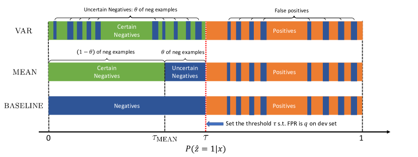
Figure 1. Illustration showing the concepts in an uncertainty-informed decision framework.

To identify high-uncertainty examples that are likely to be false negative decisions, we use an uncertainty metric $U$ to rank the negative examples. To ease later exposition, here we suppose that an ensemble model of size $T$ is used, and denote the predictions of individual ensemble members on $x_{i}$ as $y_{i}^{(1)},y_{i}^{(2)},\ldots,y_{i}^{(T)}$. The uncertainty metric $U:\mathbb{R}^{K}\rightarrow\mathbb{R}$ takes as input the ensemble predictions $\{\hat{y}_{i}^{(k)}\}$ on $x_{i}$, and outputs an real-valued uncertainty score $u(x_{i})\doteq U\left(y_{i}^{(1)},y_{i}^{(2)},\ldots,y_{i}^{(T)}\right)$. To resolve a dichotomy between “uncertain” and “certain”, we introduce a threshold $\tilde{u}$ on $u(x)$: if $u(x)>\tilde{u}$ then $x$ is deemed an uncertain input example and otherwise a certain one. We then need external resources such as human experts to inspect these uncertain negatives and determine their true states; however, due to budget constraints such resources are often limited. Therefore, we need to control the fraction of uncertain negatives. We define the uncertain negative ratio as the fraction of uncertain examples among negative examples, and bound the ratio to be below a level of $\theta$ on the development set. To evaluate how the identified uncertain negatives overlap with the actual false negatives, we use the following performance measure. The

Definition 2.1 (False Negative Precision (Jin et al., view)).

We define the false negative precision to be the fraction of false negatives among identified uncertain negative inputs by a given uncertainty metric $U$ and uncertain negative ratio $\theta$. Written in mathematical form,

(3) $$\text{FN-precision}(U,q)\doteq\frac{\left|\left\{x_{i}\,|\,i\in\mathcal{I}^{-}_{q},z_{i}=1\right\}\right|}{\left|\mathcal{I}^{-}_{q}\right|}\in[0,1],$$

where $\mathcal{I}^{-}_{q}$ is the index set of identified uncertain negative examples.

The FN-precision metric can be interpreted as the ratio of identified uncertain examples being actual false negatives. The higher the FN-precision value, the fewer false alarms are raised by $(U,q)$. We can similarly define a “false negative recall” metric that measures the fraction of false negatives identified by the algorithm; however, in this study we choose to directly report the total number of false negatives instead. In our empirical study to be described later, we will compare two commonly used uncertainty metrics, mean and var, to see which one is more suitable for the fault detection task under domain shift.

3. Methodology

Validation is a classic and almost a must-have procedure for model selection in a modern ML pipeline. The goal of validation is to obtain an accurate estimate of a trained model’s prediction performance on the test set, under the typical assumption that the training set and the test set are sampled from the same data distribution. By using validation during a model selection procedure, we can reject model instances that overfit to the training data or lead to unsatisfactory performance.

Holdout validation (hereinafter abbreviated as “holdout”) is one of the simplest validation strategies in ML. Part of the development set data is held out as the validation set, and the rest is used for training the models. The holdout validation involves only a single run, and hence part of the data is never used for training and may cause misleading results. Cross-validation alleviates the problem by involving multiple validation runs, and then combine the results of the runs together (to be discussed in details in Sec. 3.1.1). The $k$-fold cross-validation method (hereinafter abbreviated as “$k$-fold”) partitions the development set data into $k$ equal-sized folds. In a rotated fashion, each time a fold is held out as the validation set and the rest is used for training. Under both holdout and $k$-fold strategies, the development set is split randomly into a training set and a validation set. Since the split is random, we can expect that the $K^{\text{i.d.}}$ subgroups of the development set will all be represented in both the training and the validation set. If the cross-validation procedure is properly implemented, we can expect the resulting model will perform well on the i.d. data, i.e. these $K^{\text{i.d.}}$ subgroups in the development set. However, such cross-validation strategy does not take into account the resulting model’s generalization behavior on o.o.d. test data, and therefore the resulting classifier may not perform well on $\mathcal{D}_{\text{test}}^{\text{o.o.d.}}$.

3.1. Stratification-Aware Cross-Validation (SACV) Strategy for Model Selection

To address the issue mentioned above, we propose a Stratification-Aware Cross-Validation (SACV) strategy that explicitly emphasizes and prioritizes the model’s generalization performance on test data under domain shift. When an SACV strategy is employed, one by one, a subgroup (stratum) of the development set data is selected as the o.o.d. validation set; then part of the rest $K^{\text{i.d.}}-1$ subgroups will be used as the training set, and the remaining portion will be used as the i.d. validation set, as illustrated in Fig. 2.

A different technique with similar name is the stratified $k$-fold cross-validation, which also deals with stratified data but should not be confused with our proposed SACV strategy. In stratified $k$-fold cross-validation, the folds are made by preserving the portion of samples for each class (or stratum). As a result, instead of returning randomly sampled folds, stratified $k$-fold cross-validation returns stratified folds. Similar to stratified $k$-fold cross-validation, our proposed strategy also takes data stratification into consideration; however, we deliberately exclude one or more stratum from the training set and keep them solely in the validation set so that we can directly measure a trained model’s generalization performance at training time.

The primary objectives of cross-validation are 1) assessing model validity and 2) hyperparameter tuning. During cross-validation, we search through the hyperparameter space and evaluate the performance of each configuration. Suppose a total of $R$ hyperparameter configurations, respectively denoted by $\mathcal{H}_{1},\mathcal{H}_{2},\ldots,\mathcal{H}_{R}$, are evaluated and ranked during cross-validation. In our empirical study, we will retain the top-$r$ hyperparameter configurations, instead of the single best-performing one, and report their performance indices.

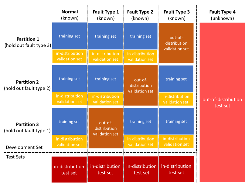
Figure 2. An illustration showing how SACV partitions a dataset during cross-validation. In this example, the dataset is made up of four fault types (subgroups), and three out of the four appear in the development set. Our goal is to train a classifier using the development set data to achieve good detection performance on both the unseen i.d. (dark red) and the o.o.d. (light red) test data.

3.1.1. Combining Results from Multiple Validation Runs

To finalize model selection, the conventional method (hereinafter referred to as refit-all) is to refit the model using the entire development set data and the selected hyperparameter configuration $\mathcal{H}^{\ast}$. Another method is to combine the $K^{\text{i.d.}}$ models, e.g., by using simple average, that are created during cross-validation in a ensemble. The idea is similar to sample Bagging (Breiman, 1996); as a result, we will name this approach combine. Later, we will compare refit-all and combine in our empirical study.

3.2. Ensemble Learning and Uncertainty Estimation

It has long been observed that ensemble learning, a meta-learning method that combines the predictions of multiple diversified learners, can help boost the prediction performance of ML models. In addition, recent literature shows that ensemble models can also be used for estimating prediction uncertainties, which is crucial for us to decide whether or not to trust the decisions made by ML models.

Diversity is recognized as one of the key factors that contribute to the success of ensemble approaches (Brown et al., 2005); the diversity allows individual classifiers to generate different decision boundaries. As illustrated in Fig. 3, the diversity among ensemble members is crucial for improving the detection performance on o.o.d. data instances. For the ensemble methods to work, the individual classifiers must exhibit diversity among themselves, such that the resulting ensemble can hopefully give a high prediction uncertainty on o.o.d. data points.

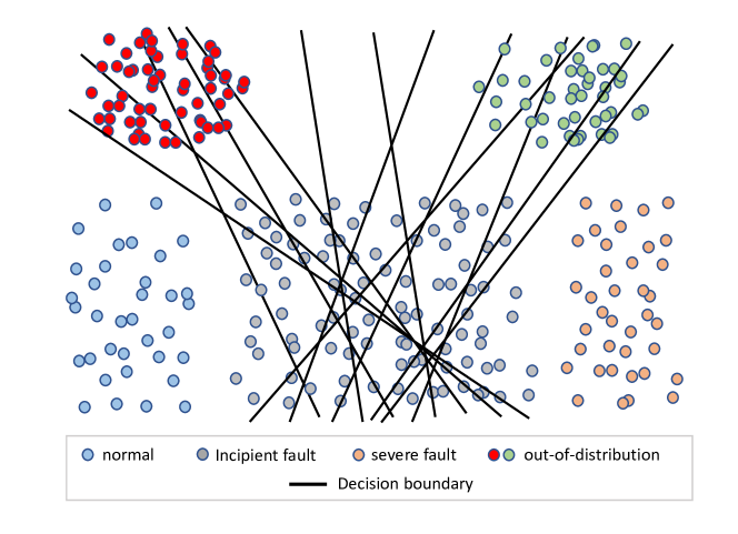
Figure 3. An illustration showing how ensemble classifiers help detect incipient fault data (Jin et al., view; Tan et al., 2020) and o.o.d. fault data.

In our empirical study to be described later, we employed the bagging (Breiman, 1996) (or bootstrap aggregation) approach for creating diversity among ensemble members. The core idea is to construct a family of models by randomly subsetting the development set (a.k.a. sample bagging (Breiman, 1996)). A later variant called feature bagging (Ho, 1998) selects a random subset of the features for training each member classifier in an ensemble. One famous application of Bagging in ML is the Random Forest (RF) model. In our empirical study, we only used sample bagging for inducing diversity among ensemble classifiers. In this study, only homogeneous base learners, i.e. models of the same type, are used to construct ensembles. The case of heterogeneous ensembles is an interesting setting and we leave it for future investigation.

Next, we will briefly introduce ensemble mean (hereinafter referred to as mean) and ensemble variance (hereinafter referred to as var), the two commonly used uncertainty metrics to be compared and evaluated in this paper.

Ensemble Mean (mean)

An intuitive metric that measures the confidence of a classifier on input $x$ is to see how close the prediction $\hat{y}$ is to the decision threshold $\tau$; same with an ensemble classifier that outputs a prediction $\hat{y}^{e}$ by combining the individual classifier’s predictions. Here we use the superscripts in $\hat{y}^{e}$ and $\tau^{e}$ to signify values associated with an ensemble classifier; in the special case where $K=1$, the ensemble classifier degenerates to a single learner model. The smaller the gap $\left|\hat{y}_{i}^{e}-\tau^{e}\right|$ is, the higher the uncertainty with $x_{i}$. Since we prefer the convention that larger function values of $u^{\textsc{mean}}(x_{i})$ corresponds to larger uncertainties, we define the uncertainty score under the margin metric can be formulated as

(4) $$u^{\textsc{mean}}(x_{i})\doteq 1-\left|\hat{y}_{i}^{e}-\tau^{e}\right|,$$

where a constant $1$ is added to the definition so that the uncertainty value $u^{\textsc{mean}}(x)$ is always positive. Since the ensemble prediction $\hat{y}_{i}^{e}$ is obtained by taking the average of the individual outputs of classifiers in the ensemble, we will hereinafter refer to this metric as mean.

Ensemble Variance (var)

The variance (or standard deviation) metric (Leibig et al., 2017; Jin et al., 2019) measures how spread out the individual learners’ predictions are from the ensemble prediction $\hat{y}_{i}^{e}$. The uncertainty score of input $x_{i}$ based on sample variance can be written as

(5) $$u^{\textsc{var}}(x_{i})\doteq\frac{1}{K-1}\sum_{k=1}^{K}\left[\hat{y}_{i}^{(k)}-\hat{y}_{i}^{e}\right]$$

A problem with var is that it focuses mainly on the disagreement among ensemble predictions but do not take in consideration the magnitude of $\hat{y}_{i}^{e}$. Consider a scenario where the all ensemble members predict a probability of $0.5$. Both var and kl will produce an uncertainty score of $0$ and thus will not be able to capture any decision uncertainties; in fact, this case where all learners give an output of $0.5$ is highly uncertain.

A theoretical analysis for comparing between the two uncertainty metrics mean and var is given in our previous works (Tan et al., 2020; Jin et al., view), but on uncertain examples known as incipient anomalies that exhibit mild symptoms of known anomaly (faults or diseases) types. The results showed that mean is a more robust uncertainty metric than var in the sense that the performance lower bound given by mean is higher than that of var. It is still unclear which uncertainty metric is likely to perform better on o.o.d. strata; we plan to give an answer to this question in our empirical study to be presented later.

We show in Fig. 4 the relationship among the various concepts introduced above. Note that techniques on different axes are orthogonal, and thus can be applied together.

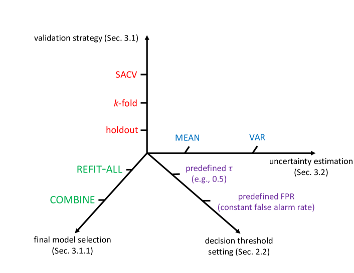
Figure 4. An illustration showing the concepts and techniques compared in this study. Orthogonal concepts are put onto different axes.

4. Datasets

In this section, we give a brief overview of the three datasets to be used in our empirical study; further details about the three datasets will be given in the appendix. We will also describe how we partitioned the datasets in our experiments into development sets and test sets.

ASHRAE RP-1043 Chiller Faults Dataset (“chiller dataset”)

We used the ASHRAE RP-1043 Dataset (Comstock and Braun, 1999) to examine the proposed approach. In the chiller dataset, sensor measurements of a 90-ton centrifugal water-cooled chiller were recorded under both fault-free and various fault conditions. In this study, we included the six faults (FT-FWE, FT-FWC, FT-RO, FT-RL, FT-CF, FT-NC) used in our previous study (Jin et al., 2019) as the fault (positive) class.

ASHRAE RP-1312 AHU Faults Dataset (“AHU dataset”)

Another important component of a building Heating, Ventilation and Air Conditioning (HVAC) system is the AHU whose functionality is to regulate and circulate air to the indoor zones in a building. Our study included 25 commonly encountered AHU faults (eleven in spring, eight occur in summer, and six in winter). By treating data from each season as an independent dataset, we will then have three sub-datasets, namely AHU-spring, AHU-summer and AHU-winter, for our experimental study. We adopted the features selected by Li et al.’s previous work (Li et al., 2017).

Power System Faults Dataset (“power dataset”)

To further validate the proposed approach, we also examined its performance on a fault dataset from another typical CPS—an electric power system. This dataset contains rich dynamic characteristics and it models the high-order complexity of the power system under High Impedance Faults. The benchmark system that generates the HIFs has a variety of system configurations under different distributed energy resource technologies such as synchronous machines and inverter-interfaced renewable generators. Based on this benchmark system, we have created three sub-datasets for 1) faults occurred in three locations 2) faults resulting from six impedance values, and 3) faults of four different types (single-line-to-ground faults, line-to-line faults, line-to-line-to-ground faults, and three-phase faults); details of the dataset can be found in (Cui et al., 2019). We will refer to the three sub-datasets respectively as power-loc, power-res, and power-ft.

4.1. Dataset Partitioning

To study the generalization performance of different cross-validation methods, we performed a series of experiments on each dataset. For each dataset consisting of $K$ subgroups, we repeated the experiment for $K$ times, each time leaving out a different subgroup as the o.o.d. test set. The i.d. test set is then partitioned out of the rest $K^{\text{i.d.}}=K-1$ subsets. The remaining data will constitute the development set.

5. Experimental Details

5.1. Experiment Setup

We conducted the experiments on all three datasets described above in Sec. 4. Decision Tree (DT) and Neural Network (NN) models were used as base learners in our experimental study, and then combined them together into Bagging ensembles (Breiman, 1996). We built Bagging ensembles of two different sizes $5$ and $10$, and used the single learner case as the baseline. For each experiment, we excluded one subgroup from the whole dataset and use it as the o.o.d. test data, as described earlier in Sec. 4.1. To induce diversity, we swept a wide range of hyperparameters settings, and selected the top 5 best-performing sets of hyperparameters with which the models obtained the highest test scores. More details of our experimental setup and implementation can be found in the released code.

5.2. Comparing Final Model Selection Methods: refit-all vs. combine

We first compare the two “final model selection” methods, refit-all and combine, described in Sec. 3.1.1, by examining their performance differences on the three datasets (including all of their sub-datasets). Both give similar performance on i.d. data, and we further assess their performance in terms of the FNR on the o.o.d. data under 1) different configurations of $q$ (i.e. the predefined FPR level on the development set): $1\%$, $2\%$, $3\%$, $5\%$, $10\%$ and also 2) under $\tau=0.5$. For the three AHU sub-datasets, we only noticed significant performance differences when SP-FT-8, SU-FT-4, WT-FT-4 were used as o.o.d. data, and combine performed much better than refit-all. When the rest were used as the o.o.d. data, both refit-all and combine gave very low FNR. We observed similar phenomena with the power dataset and the chiller dataset. For the power dataset, we also achieved very low FNR under both refit-all and combine for every data subgroup was used as o.o.d. data except for FT-4, LOC-2, RES-2. For the chiller dataset, performance difference was only significant when RL and CF were held out as o.o.d. test set. Again, combine outperformed refit-all. In Fig. 5, we only displayed results for the above-mentioned cases where there was significant performance gap between refit-all and combine, and omitted the rest. The low FNR in the omitted cases may be a result of the held-out subgroups not being enough “out-of-distribution”; in other words, the held-out subgroup may resemble one or more of the i.d. subgroups which leads to high detection performance. In our upcoming analysis, we will omit these cases as well, and focus on the challenging cases where the held-out test set presents real o.o.d. challenges to fault detection models.

To sum up, it is clear that the combine method has lower FNR compared with the refit-all, indicating that the combine has a better performance in improving the models’ generalization ability. Therefore, in our next experiments, we will only display results from combine.

5.3. Comparing Validation Strategies: SACV vs. $k$-fold vs. Holdout

Next, we evaluated the ensemble methods’ performance on the o.o.d. data when different validation strategies are used. As in the previous experiment, we examined the FNRs across different configurations of $\tau$ (by directly setting $\tau=0.5$ or varying $q$). For comparison, we used the holdout validation and the $k$-fold cross-validation as our baselines. The number of splits used in $k$-fold cross-validation is set to be equal to the number of classes of the development set, i.e. $k=K^{\text{i.d.}}$. We visualized the results from same subgroups as introduced in the previous analysis. The results can be found in Fig. 6.

Comparing the three validation strategies, we can clearly see in Fig. 6 that SACV achieved significant improvement in FNR over the other two validation strategies, indicating that SACV is indeed effective in improving the models’ generalization performance. In Fig. 6, we only showed the results for a selected number of cases where baseline methods performed poorly on the held out o.o.d. data, and omitted the rest since the baseline FNRs for these omitted cases are already close to zero. In addition, we can also see from the results that the FNRs decrease with the increment of fixed q.

5.4. Comparing Uncertainty Metrics: mean vs. var

Finally, we compared the different metrics used for uncertainty estimating including: 1) mean, 2) var, described in Sec. 3.2. We evaluated our models’ generalization performance by calculating the number of remaining false negatives after applying uncertainty estimation, assuming all of the identified false negatives can be corrected perfectly by human experts.

The results given by mean and by var, as well as the performance baseline where no uncertainty estimation is applied (baseline), are displayed in Fig. 7. As illustrated in the plots, it is clear that both mean and var metrics have decent improvement in identifying false negatives over baseline. Specifically, comparing mean and var, we also found that var outperformed mean, indicating that var excelled at estimating o.o.d. data.

Another finding is the RF has larger improvement as the ensemble size grows, compared to NN. One possible reason for this is that single NN classifiers have stronger classification abilities over single DTs classifiers.

The above results seem to contradict the conclusion from our previous work (Tan et al., 2020; Jin et al., view), where we showed that mean is more preferable to var for identifying incipient anomalies (faults or diseases). It is worth mentioning that our focus in this paper is o.o.d. fault data that are not included in the development set during training, rather than incipient faults. We illustrate the differences between the two scenarios in Fig. 3, and how ensemble methods can help with fault detection in both scenarios. It will be interesting future work to understand why var excels at identifying o.o.d. data.

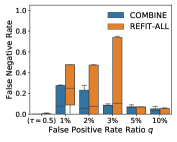
(a) RF: chiller (FT-RL)

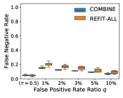
(b) NN: chiller (FT-RL)

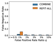
(c) RF: chiller (FT-CF)

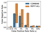
(d) NN: chiller (FT-CF)

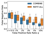
(e) RF: AHU (SP-FT-8)

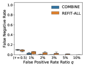
(f) NN: AHU (SP-FT-8)

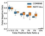
(g) RF: power (FT-4)

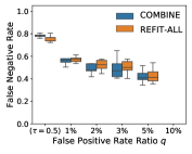
(h) NN: power (FT-4)

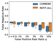
(i) RF: AHU (SU-FT-4)

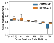
(j) NN: AHU (SU-FT-4)

(k) RF: power (LOC-2)

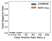
(l) NN: power (LOC-2)

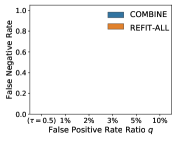
(m) RF: AHU (WT-FT-2)

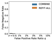
(n) NN: AHU (WT-FT-2)

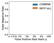
(o) RF: power (RES-2)

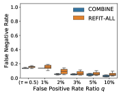
(p) NN: power (RES-2)

Figure 5. Performance comparison between the refit-all and the combine methods in terms of their FNR on different datasets are presented: 1) the chiller dataset, 2) the AHU dataset, and 3) the power dataset. The excluded subgroup that is used as the o.o.d. test set and SACV is used as the cross-validation method.

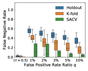
(a) RF: chiller (FT-RL)

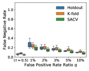
(b) NN: chiller (FT-RL)

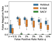
(c) RF: chiller (FT-CF)

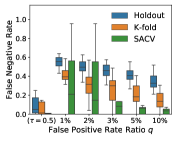
(d) NN: chiller (FT-CF)

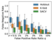
(e) RF: AHU (SP-FT-8)

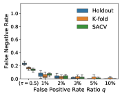
(f) NN: AHU (SP-FT-8)

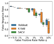
(g) RF: power (FT-4)

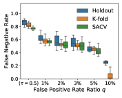
(h) NN: power (FT-4)

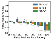
(i) RF: AHU (SU-FT-4)

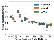
(j) NN: AHU (SU-FT-4)

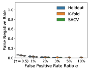
(k) RF: power (LOC-2)

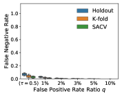
(l) NN: power (LOC-2)

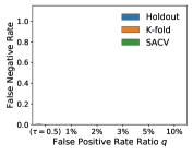
(m) RF: AHU (WT-FT-2)

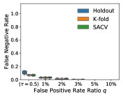
(n) NN: AHU (WT-FT-2)

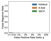
(o) RF: power (RES-2)

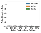
(p) NN: power (RES-2)

Figure 6. The FNR given by different (cross-)validation methods: 1) holdout, 2) $k$-fold, and 3) SACV. Results from RF and NN on different datasets are presented: 1) the chiller dataset, 2) the AHU dataset and 3) the power dataset.

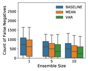
(a) RF: chiller (FT-RL)

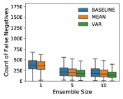
(b) NN: chiller (FT-RL)

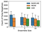
(c) RF: chiller (FT-CF)

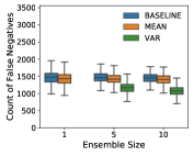
(d) NN: chiller (FT-CF)

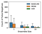
(e) RF: AHU (SP-FT-8)

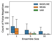
(f) NN: AHU (SP-FT-8)

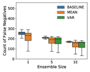
(g) RF: power (FT-4)

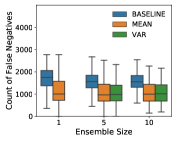
(h) NN: power (FT-4)

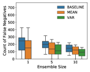
(i) RF: AHU (SU-FT-4)

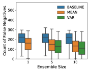
(j) NN: AHU (SU-FT-4)

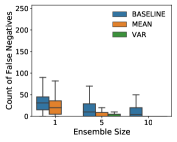
(k) RF: power (LOC-4)

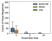
(l) NN: power (LOC-4)

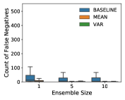
(m) RF: AHU (WT-FT-4)

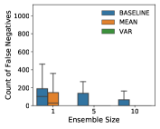
(n) NN: AHU (WT-FT-4)

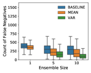
(o) RF: power (RES-2)

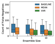
(p) NN: power (RES-2)

Figure 7. The count of remaining false negatives under different uncertainty metrics: 1) baseline ($\theta=0$, i.e. no uncertainty information is exploited), 2) mean and 3) var. The results from tree ensembles (RFs) and NN ensembles on the three datasets are presented.

6. Related Work

6.1. Adversarial Validation

A closely related technique that also deals with the domain shift phenomenon between training and test distributions is the adversarial validation approach (Pan et al., 2020) whose goal is to detect and address the difference between the training and test datasets. The idea of adversarial validation is to create an adversarial validation set as an proxy of the test set for selecting robust models during training such that the resulting model can achieve satisfactory performance on the adversarial validation set (and hopefully on the test set as well).

The creation of effective adversarial validation sets, however, will usually require prior information about the test data distribution. In some occasions, for example in Kaggle competitions, part of the test set data is made public at training time while the rest is used as a “private test set”. In adversarial validation approaches, a classifier is trained to distinguish the training and the (public) test set data, and then part of the training data (e.g., the difficult-to-classify ones) that resembles the test data can be held out as an adversarial validation set. Such approach is described as the “validation data selection” method in Pan et al.’s recent work (Pan et al., 2020), which also describes other types of adversarial validation methods; see details therein for further information.

In fact, the “public test set” data mentioned above can also be considered as part of the development set (because the public test set data are available at training time), and thus not actually a “real” test set. In situations where little information about the test data distribution is available, adversarial validation will not be applicable. Our SACV approach does not require prior information about the unseen test distribution. Instead, this approach rely only on the available development set data. By holding out one fault subgroup (stratum) at a time, we seek to build a model that is most robust against possible adversarial fault examples.

6.2. Out-of-Distribution Data Detection

In recent years, a number of research papers (Lakshminarayanan et al., 2017; Gal, 2016) related to the detection of o.o.d. data are seen in literature. Lakshminarayanan et al. (Lakshminarayanan et al., 2017) proposed using random initialization and random shuffling of training examples to diversify base learners of the same network architecture. Gal and Ghahramani proposed using MC-dropout (Gal, 2016) to estimate a network’s prediction uncertainty by using dropout not only at training time but also at test time. By repeatedly sampling a dropout model $\mathcal{M}$ using the same input for $T$ times, we can obtain an ensemble of prediction results with $T$ individual probability vectors. The dropout technique provides an inexpensive approximation to training and evaluating an ensemble of exponentially many similar yet different neural networks.

6.3. Incipient Anomaly Detection

Another application of decision uncertainty and ensemble methods is the detection of incipient anomalies (e.g., industrial machine faults and human diseases). Incipient anomalies (Jin et al., 2019) present milder symptoms compared to severe ones, and can be easily mistaken as the normal operating conditions due to their close resemblance to normal operating conditions. The lack of incipient anomaly examples in the training data can pose severe risks to anomaly detection methods that are built upon ML techniques. To address this challenge, the authors of (Jin et al., 2019; Jin et al., 2020; Tan et al., 2020) propose to utilize the uncertainty information from ensemble learners to identify potential misclassified incipient anomalies, and show that the uncertainty-informed detection scheme gives improved results on incipient anomalies without sacrificing performance on non-incipient anomaly examples.

7. Conclusion

In this paper, we showed that domain shift in stratified data can undermine fault detection performance, especially when some subgroups (strata) appear in the test data distribution but not in the training distribution. We proposed an easy-to-use cross-validation method to mitigate the issue and demonstrated its efficacy on three representative CPS datasets. Our proposed SACV approach achieved significant performance improvement over traditional holdout and $k$-fold validation methods on o.o.d. data, in the meantime without sacrificing its performance on i.d. data. For future work, we plan to extend the proposed methodology to datasets of different modalities, such as image data.

Appendix A RP-1043 Chiller Dataset

The RP-1043 chiller dataset (Comstock and Braun, 1999) is not public but is available for purchase from ASHRAE. The 90-ton chiller studied in the RP-1043 chiller dataset is representative of chillers used in larger installations (MC and JE, 2002), and consisted of the following parts: evaporator, compressor, condenser, economizer, motor, pumps, fans, and distribution pipes etc. with multiple sensor mounted in the system. Fig. 8 depicts the cooling system with sensors mounted in both evaporation and condensing circuits.

The same sixteen features and six fault types as used in our previous work (Tan et al., 2019) were used to train our models in our empirical study. We also attempted to use other sets of selected features than the sixteen features in our case study, e.g., the features identified in Li et al.’s previous work (Li et al., 2016), and similar results were obtained. Table 1 and Table 2 give detailed descriptions of the sixteen features and the six fault types used in this study, respectively. In the chiller dataset, each fault was introduced at four Severity Levels, and we included fault data of all four SLs in the dataset for our experiment. The condenser fouling (FT-CF) fault was emulated by plugging tubes into condenser. The reduced condenser water flow rate (FT-FWC) fault and reduced evaporator water flow rate (FT-FWE) fault were emulated directly by reducing water flow rate in the condenser and evaporator. The refrigerant overcharge (FT-RO) fault and refrigerant leakage (FT-RL) fault were emulated by reducing or increasing the refrigerant charge respectively. The excess oil (FT-EO) fault was emulated by charging more oil than nominal. And the non-condensable in refrigerant (FT-NC) fault was emulated by adding Nitrogen to the refrigerant.

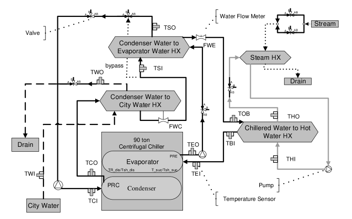
Figure 8. A schematic of the cooling system test facility and sensors mounted in the related water circuits (Li, 2017).

Table 1. Descriptions of variables used as features in the chiller dataset

Sensor	Description	Unit
TEI	Temperature of entering evaporator water	°F
TEO	Temperature of leaving evaporator water	°F
TCI	Temperature of entering condenser water	°F
TCO	Temperature of leaving condenser water	°F
Cond Tons	Calculated Condenser Heat Rejection Rate	Tons
Cooling Tons	Calculated City Water Cooling Rate	Tons
kW	Compressor motor power consumption	kW
FWC	Flow Rate of Condenser Water	gpm
FWE	Flow Rate of Evaporator Water	gpm
PRE	Pressure of refrigerant in evaporator	psig
PRC	Pressure of refrigerant in condenser	psig
TRC	Subcooling temperature	°F
T_suc	Refrigerant suction temperature	°F
Tsh_suc	Refrigerant suction superheat temperature	°F
TR_dis	Refrigerant discharge temperature	°F
Tsh_dis	Refrigerant discharge superheat temperature	°F

Table 2. The six chiller faults in our study

Fault Types	Identity	Normal Operation
Reduced Condenser Water Flow	FT-FWC	270 gpm
Reduced Evaporator Water Flow	FT-FWE	216 gpm
Refrigerant Leak	FT-RL	300 lb
Refrigerant Overchange	FT-RO	300 lb
Condenser Fouling	FT-CF	164 tubes
Non-condensables in System	FT-NC	No nitrogen

Appendix B RP-1312 AHU Dataset

The AHU dataset included 16 fault types in total that are distributed across three seasons: spring, summer and winter. A detailed list of the 16 fault types studied by the AHU dataset is given in Table 3, where each fault is assigned a unique identifier. We can also see that the faults appearing in different seasons do not fully overlap; there are faults that exist only in spring but not in summer or winter (e.g., SP-FT-1) and also faults that appear in all three seasons such as the “exhaust air damper stuck” fault. When building ML models for each season, we only considered faults that appear in that season. For example, the fault (positive) class for the AHU-spring dataset encompasses $11$ faults; these fault types constituted the $11$ subgroups (strata) in the fault class.

The schematic of a typical AHU system is shown in Fig. 9(a) that is configured for a Variable Air Volume (VAV) system. The VAV system maintains the supply air temperature to the terminals for air-conditioning. The testing site for creating the RP-1312 AHU Dataset involved two AHUs, i.e., AHU-A and AHU-B as shown in Fig. 9(b) that were operated under real weather and building load conditions. Faults were manually introduced into the air-mixing box, the coils, and the fan sections of AHU-A (treatment group), while AHU-B was operated at nominal states to serve as the control group.

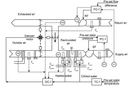
(a) AHU system schematic

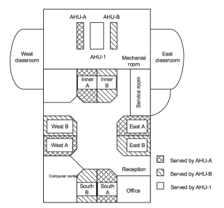
(b) RP-1312 testing site layout

Figure 9. We show in (a) a typical single-duct VAV AHU system (Li, 2017), and in (b) the schematic of the testing site used for creating the RP-1312 AHU Dataset (Wen and Li, 2012).

Table 3. Fault Types Studied in the RP-1312 AHU Dataset

Fault Types	Spring	Summer	Winter
Outside air damper leak		SU-FT-1	WT-FT-1
Outside air temperature sensor bias	SP-FT-1
Outside air damper stuck	SP-FT-2		WT-FT-2
Exhaust air damper stuck	SP-FT-3	SU-FT-2	WT-FT-3
Cooling coil valve control unstable	SP-FT-4	SU-FT-3
Cooling coil valve reverse action		SU-FT-4
Cooling coil valve stuck	SP-FT-5	SU-FT-5	WT-FT-4
Heating coil valve leaking		SU-FT-6
Return fan at fixed speed	SP-FT-6	SU-FT-7
Return fan complete failure	SP-FT-7	SU-FT-8
Air filter area block fault	SP-FT-8
Mixed air damper unstable	SP-FT-9
Sequence of heating and cooling unstable	SP-FT-10
Supply fan control unstable	SP-FT-11
Heating coil fouling			WT-FT-5
Heating coil reduced capacity			WT-FT-6

Appendix C Power System Faults Dataset

The benchmark system that generates this dataset can be found in Fig. 10. In this system, we simulate three system configuration under different distributed energy resource (DER) technologies, namely, synchronous-machine-based-system (synchronous machine at location A), inverter-based system (the inverter-interfaced wind farm at location A), and the hybrid system (synchronous machine at location A and the inverter-interfaced wind farm at location B). The wind farm is type 4 and rated at 575 V, 6.6 MVA. According to IEEE Standard 1547, the wind farm adopts constant power control with LVRT capability. The maximum fault current is limited to $1.5$ pu.

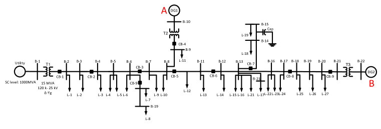
Figure 10. A single line diagram of the distribution feeder under study (Cui et al., 2019).

Table 4 lists the event category and event type under study. The event numbers are explained as follows. First, $8$ loading conditions and $3$ DER technologies are examined respectively on top of the base case scenario. Furthermore, the $10$ events from Type 1 is associated with the undowned conductor, where $3$ SLG (AG, BG, CG), $3$ LLG (ABG, ACG, BCG), $3$ LL (AB, BC, AC), and $1$ LLLG (ABCG) faults are included. The $3$ events of Type 2 fault are the downed conductor for each phase. The fault impedance values includes $50,150,250,350,450$, and $550\text{\,}\Omega$ in this paper. In load switching, the $6$ types of non-fault events include $4$ single load switching (L-4, L-9, L-19, L-23) and $2$ combinational load switching ((L-2,L-4,L-5) and (L-9, L-10)) events. Additionally, the $2$ capacitor switching events have both the on and off status of the capacitor bank near bus B-15. A loading condition ranging from $30\%$ to $100\%$, in a step of $10\%$, is simulated.

Table 4. Event Category of the System Under Study (Cui et al., 2019).

Event Category	Event Type	Event Nunber
System Operating Condition	Loading Condition (30%-100%)	8
	DER Tech. (SG, inverter, hybrid)	3
Fault Event	Type 1: SLG, LLG, LL, LLLG	10
	Type 2: Downed conductor	3
	Fault impedance	6
	Inception Angle ($0\text{\,}\mathrm{\SIUnitSymbolDegree}$, $30\text{\,}\mathrm{\SIUnitSymbolDegree}$, $60\text{\,}\mathrm{\SIUnitSymbolDegree}$, $90\text{\,}\mathrm{\SIUnitSymbolDegree}$)	4
	Fault location	3
Non-fault Event	Normal State	1
	Load Switching	6
	Capacitor Switching	2

References

- (1)
- Breiman (1996) Leo Breiman. 1996. Bagging predictors. Machine learning 24, 2 (1996), 123–140.
- Brown et al. (2005) Gavin Brown, Jeremy Wyatt, Rachel Harris, and Xin Yao. 2005. Diversity creation methods: a survey and categorisation. Information Fusion 6, 1 (2005), 5–20.
- Chong et al. (2011) Ui-Pil Chong et al. 2011. Signal model-based fault detection and diagnosis for induction motors using features of vibration signal in two-dimension domain. Strojniški vestnik 57, 9 (2011), 655–666.
- Comstock and Braun (1999) MC Comstock and JE Braun. 1999. Development of analysis tools for the evaluation of fault detection and diagnostics in chillers. ASHRAE Research Project RP-1043. American Society of Heating, Refrigerating and Air-Conditioning Engineers, Inc., Atlanta. Also, Report HL (1999), 99–20.
- Cui et al. (2019) Qiushi Cui, Khalil El-Arroudi, and Yang Weng. 2019. A feature selection method for high impedance fault detection. IEEE Transactions on Power Delivery 34, 3 (2019), 1203–1215.
- Gal (2016) Yarin Gal. 2016. Uncertainty in deep learning. University of Cambridge (2016).
- Harihara et al. (2003) Parasuram P Harihara, Kyusung Kim, and Alexander G Parlos. 2003. Signal-based versus model-based fault diagnosis-a trade-off in complexity and performance. In 4th IEEE International Symposium on Diagnostics for Electric Machines, Power Electronics and Drives, 2003. SDEMPED 2003. IEEE, 277–282.
- Ho (1998) Tin Kam Ho. 1998. The random subspace method for constructing decision forests. IEEE transactions on pattern analysis and machine intelligence 20, 8 (1998), 832–844.
- Isermann (2005) Rolf Isermann. 2005. Model-based fault-detection and diagnosis–status and applications. Annual Reviews in control 29, 1 (2005), 71–85.
- Jayaprakash and Choon (2008) Saththasivam Jayaprakash and Ng Kim Choon. 2008. Predictive and diagnostic methods for centrifugal chillers. ASHRAE Trans 114, 1 (2008), 282–287.
- Jia et al. (2018) R. Jia, B. Jin, M. Jin, Y. Zhou, I. C. Konstantakopoulos, H. Zou, J. Kim, D. Li, W. Gu, R. Arghandeh, P. Nuzzo, S. Schiavon, A. L. Sangiovanni-Vincentelli, and C. J. Spanos. 2018. Design Automation for Smart Building Systems. Proc. IEEE 106, 9 (Sept 2018), 1680–1699. https://doi.org/10.1109/JPROC.2018.2856932
- Jianying and Shengwei (2005) Qin Jianying and Wang Shengwei. 2005. A fault detection and diagnosis strategy of VAV air-conditioning systems for improved energy and control performances. Energy and Buildings 37, 10 (2005), 1035–1048.
- Jifeng and Rong (2008) Ru Jifeng and Li X Rong. 2008. Variable-structure multiple-model approach to fault detection, identification, and estimation. IEEE Transactions on Control Systems Technology 16, 5 (2008), 1029–1038.
- Jin et al. (2019) Baihong Jin, Dan Li, Seshadhri Srinivasan, See-Kiong Ng, Kameshwar Poolla, and Alberto Sangiovanni-Vincentelli. 2019. Detecting and diagnosing incipient building faults using uncertainty information from deep neural networks. In 2019 IEEE International Conference on Prognostics and Health Management (ICPHM). IEEE, 1–8.
- Jin et al. (2020) Baihong Jin, Yingshui Tan, Yuxin Chen, and Kameshwar Poolla. 2020. Are Ensemble Classifiers Powerful Enough for the Detection and Diagnosis of Intermediate-Severity Faults? arXiv preprint arXiv:2007.03167 (2020).
- Jin et al. (view) Baihong Jin, Yingshui Tan, Albert Liu, Xiangyu Yue, Yuxin Chen, and Alberto L. Sangiovanni-Vincentelli. under review. Using Ensemble Classifiers to Detect Incipient Anomalies. ACM Transactions on Cyber-Physical Systems (under review).
- Lakshminarayanan et al. (2017) Balaji Lakshminarayanan, Alexander Pritzel, and Charles Blundell. 2017. Simple and scalable predictive uncertainty estimation using deep ensembles. In Advances in Neural Information Processing Systems. 6402–6413.
- Leibig et al. (2017) Christian Leibig, Vaneeda Allken, Murat Seçkin Ayhan, Philipp Berens, and Siegfried Wahl. 2017. Leveraging uncertainty information from deep neural networks for disease detection. Scientific reports 7, 1 (2017), 17816.
- Li (2017) Dan Li. 2017. Fault detection and diagnosis for chillers and AHUs of building ACMV systems. Ph.D. Dissertation.
- Li et al. (2016) Dan Li, Yuxun Zhou, Guoqiang Hu, and Costas J Spanos. 2016. Fault detection and diagnosis for building cooling system with a tree-structured learning method. Energy and Buildings 127 (2016), 540–551.
- Li et al. (2017) D. Li, Y. Zhou, G. Hu, and C. J. Spanos. 2017. Optimal Sensor Configuration and Feature Selection for AHU Fault Detection and Diagnosis. IEEE Transactions on Industrial Informatics 13, 3 (2017), 1369–1380.
- Li and Wen (2014) Shun Li and Jin Wen. 2014. A model-based fault detection and diagnostic methodology based on PCA method and wavelet transform. Energy and Buildings 68 (2014), 63–71.
- Luo et al. (2019) Yawei Luo, Liang Zheng, Tao Guan, Junqing Yu, and Yi Yang. 2019. Taking a closer look at domain shift: Category-level adversaries for semantics consistent domain adaptation. In Proceedings of the IEEE Conference on Computer Vision and Pattern Recognition. 2507–2516.
- MC and JE (2002) Comstock MC and Braun JE. 2002. Fault detection and diagnostic (FDD) requirements and evaluation tools for chillers. ASHRAE (2002).
- Pan et al. (2020) Jing Pan, Vincent Pham, Mohan Dorairaj, Huigang Chen, and Jeong-Yoon Lee. 2020. Adversarial Validation Approach to Concept Drift Problem in Automated Machine Learning Systems. arXiv preprint arXiv:2004.03045 (2020).
- Richards (2005) Mark A Richards. 2005. Fundamentals of radar signal processing. Tata McGraw-Hill Education.
- Sun et al. (2020) Yu Sun, Xiaolong Wang, Zhuang Liu, John Miller, Alexei A Efros, and Moritz Hardt. 2020. Test-time training with self-supervision for generalization under distribution shifts. In International Conference on Machine Learning (ICML).
- Tan et al. (2019) Yingshui Tan, Baihong Jin, Alexander Nettekoven, Yuxin Chen, Yisong Yue, Ufuk Topcu, and Alberto Sangiovanni-Vincentelli. 2019. An Encoder-Decoder Based Approach for Anomaly Detection with Application in Additive Manufacturing. In 2019 18th IEEE International Conference On Machine Learning And Applications (ICMLA). IEEE, 1008–1015.
- Tan et al. (2020) Yingshui Tan, Baihong Jin, Xiangyu Yue, Yuxin Chen, and Alberto Sangiovanni Vincentelli. 2020. Exploiting Uncertainties from Ensemble Learners to Improve Decision-Making in Healthcare AI. ArXiv abs/2007.06063 (2020).
- Vorburger and Bernstein (2006) Peter Vorburger and Abraham Bernstein. 2006. Entropy-based concept shift detection. In Sixth International Conference on Data Mining (ICDM’06). IEEE, 1113–1118.
- Wen and Li (2012) J Wen and S Li. 2012. RP-1312–Tools for evaluating fault detection and diagnostic methods for air-handling units. Technical Report. ASHRAE, Tech. Rep.
- Wijayasekara et al. (2014) Dumidu Wijayasekara, Ondrej Linda, Milos Manic, and Craig Rieger. 2014. Mining building energy management system data using fuzzy anomaly detection and linguistic descriptions. Industrial Informatics, IEEE Transactions on 10, 3 (2014), 1829–1840.
- Xuewu and Zhiwei (2013) Dai Xuewu and Gao Zhiwei. 2013. From model, signal to knowledge: A data-driven perspective of fault detection and diagnosis. IEEE Transactions on Industrial Informatics 9, 4 (2013), 2226–2238.
- Zhiwei et al. (2015) Gao Zhiwei, Carlo Cecati, and Ding Steven X. 2015. A survey of fault diagnosis and fault-tolerant techniques-Part I: fault diagnosis With model-based and signal-based approaches. IEEE Transactions on Industrial Electronics 62, 6 (2015), 3757–3767.
- Zhou et al. (2017) Datong P Zhou, Qie Hu, and Claire J Tomlin. 2017. Quantitative comparison of data-driven and physics-based models for commercial building HVAC systems. In 2017 American Control Conference (ACC). IEEE, 2900–2906.