A new role for circuit expansion for learning in neural networks

Abstract

Many sensory pathways in the brain include sparsely active populations of neurons downstream from the input stimuli. The biological purpose of this expanded structure is unclear, but may be beneficial due to the increased expressive power the network. In this work, we show that certain ways of expanding a neural network can improve its generalization performance even when the expanded structure is pruned after the learning period. To study this setting, we use a teacher-student framework where a perceptron teacher network generates labels corrupted with small amounts of noise. We then train a student network structurally matched to the teacher. In this scenario, the student can achieve optimal accuracy if given the teacher’s synaptic weights. We find that sparse expansion of the input layer of a student perceptron network both increases its capacity and improves the generalization performance of the network when learning a noisy rule from a teacher perceptron when the expansion is pruned after learning. We find similar behavior when the expanded units are stochastic and uncorrelated with the input and analyze this network in the mean field limit. By solving the mean field equations, we show that the generalization error of the stochastic expanded student network continues to drop as the size of the network increases. This improvement in generalization performance occurs despite the increased complexity of the student network relative to the teacher it is trying to learn. We show that this effect is closely related to the addition of slack variables in artificial neural networks and suggest possible implications for artificial and biological neural networks.

I Introduction

Learning and memory is thought to occur mainly through long term modification of synaptic connections among neurons, a phenomenon well established experimentally. Additionally, neural circuits also undergo structural changes on a global level. It is observed that synaptic density in the human cortex increases rapidly after birth and then drops sharply towards adulthood, indicating an extensive pruning of the neuronal circuits Sakai (2020). Another form of structural plasticity, also occurring in the adult brain, is the continuous recycling of synapses which is seen in both cortex and hippocampus. In the past, several modeling studies have addressed the computational consequences of these phenomena (see Aimone (2016); Deng et al. (2010) for adult neurogenesis and Mongillo et al. (2017) for synaptic recycling).

In this work, we explore a novel computational benefit of structural dynamics in neural circuits that learn new associations or tasks. We show that under certain classes of learning paradigms, the expansion of a neural circuit architecture by recruiting additional neurons and synapses may facilitate the dynamics of learning. Expanding circuit sizes to enable sparse coding has been shown to have computational benefits in several contexts of neuroscience and machine learning for sensory processing, learning and memory Olshausen and Field (2004); Ganguli and Sompolinsky (2012); Litwin-Kumar et al. (2014); Treves and Rolls (1994); Tsodyks and Feigelman (1988). In these models, circuit expansion and the resultant sparse coding yield better representations of the stimuli, enhancing pattern separation, and improving the capacity for pattern retrieval and classification. Importantly, to realize these benefits, the expanded architecture needs to be stable after learning. By contrast, in our scenario, the benefit of expansion lies in its facilitating the dynamics of learning and not its information bearing potential. In fact, expansion in this scenario is most beneficial when it is transient, i.e. the added neurons and synapses are pruned after the learning period. Hence this hypothesis is consistent with the observed continuous recycling of synapses during learning.

Within this work, we consider neural networks that learn supervised classification problems implemented by a single layer perceptron. Despite the apparent simplicity of this task, learning the rule by training with labeled examples may be hampered by the complexity of the underlying data. We focus on two cases of unrealizable rules, which are characterized by a critical size of the training set above which no single layer student is able to correctly classify all of the training examples. This critical size is called the student’s capacity. We first consider unrealizable rules occurring when the teacher network produces training labels corrupted by stochastic noise and will later consider cases in which the teacher is more complex than the student network trying to learn the rule. We show that adding sparse expansions to student networks by random mappings of the original input increases the capacity of the student network and improves the generalization performance of the network as it is trained on larger training sets.

While the capacity of a network is clearly related to its dimensionality, it is not obvious and even counterintuitive that increasing the size of a network should improve its generalization performance. Using mean field theory and simulations of a wide range of network parameters, we show that expansion of the architecture during learning achieves improved generalization, particularly if the additional elements of the circuit are removed after learning. In addition, it is shown that the effect is more pronounced if the hidden representation during learning is sparse. We find that the performance is most improved when the expanded units are random and uncorrelated with the original input which suggests that having low overlap in expanded activity between different training input is crucial to improving performance.

Our analysis offers a new perspective on the important issue of the relation between model complexity and learning in neural networks. Artificial neural networks have achieved state of the art predictive performance on a variety of tasks, especially within the past decade LeCun et al. (2015); Schmidhuber (2015). The primary benefit to training these enormous models appears to lie in their ability to represent very complex functions and the link between width, depth, and expressivity of neural networks is discussed in detail in several studies including, Bengio and Delalleau (2011); Poole et al. (2016); Safran and Shamir (2017); Raghu et al. (2017). These networks are often over-parameterized in the sense that than the number of examples the network is trained on is far less than the number of free parameters in the network Simonyan and Zisserman (2014). Classical statistical learning theory suggests that such massively over-parameterized models should be expected to over-fit on the training data Zhang et al. (2017) and make poor predictions on new inputs not seen by the network before. To resolve this apparent paradox, it has been suggested that modern learning algorithms cost functions, and architectures incorporate strong explicit and implicit regularizations Bartlett and Mendelson (2002); Advani et al. (2020); Bansal et al. (2018); Mohri et al. (2012). Our findings suggest there may be advantages to making neural networks larger than is required for expressing the underlying task. These advantages are related to enhancing the ease of the learning convergence, and that in these cases, optimal performance after learning is achieved upon removal of the additional nodes and weights. Indeed, pruning of Deep Neural Networks after training is a current topic of research in machine learning Han et al. (2015); Yang et al. (2017); Blalock et al. (2020); Gale et al. (2019).

We start in section II by showing in simulations that implementing a sparse expansion of a perceptron network via random mapping of the input can improve its generalization ability when learning from a noisy teacher. In section III we analyze these results by studying a simpler model of a single layer perceptron in which the activity in the expanded units is random and uncorrelated with the stimulus. We use the replica method to derive a mean field theory exact in the thermodynamic limit, and find it matches well with simulations of large but finite size networks. In section III.2 we explain this phenomena more intuitively by showing a correspondence between adding random input neurons and including slack variables in the optimization problem. We also discuss how hidden units in our two layer network model can resemble the stochastic expansion of the input layer in the one layer model. In section IV.1 we demonstrate how the benefit of sparse expansion also applies in more general cases of learning unrealizable rules by comparing the performance of a student learning from a more complex teacher network to our theory results. In most of our work we have focused on convex learning algorithms. In section IV.2 we discuss to what extent these effects extend to other learning algorithms. Finally, we close by discussing some general implications of our results.

II Sparse Expansions and Learning

Figure 1: Teacher and student network schematics. (A) noisy teacher network (B) student network (C) Student with sparse hidden layer (D) Student with stochastic expanded units.

We begin our analysis by considering a teacher perceptron network with $N_{0}$ input nodes $x_{i}$, one output node $y_{0}$, and $N_{0}$ synaptic weights $w_{i}^{0}$ drawn iid from $w_{i}^{0}\sim\mathcal{N}\left(0,\sigma_{w}^{2}\right)$ and supervised learning tasks in which a student perceptron will attempt to learn the teacher’s input-output rule from a training set provided by it. For each input $x$ drawn iid from $x_{i}\sim\mathcal{N}\left(0,1\right)$, the teacher network assigns a label $y_{0}\in\{-1,1\}$ via the following rule: $y_{0}=\text{sign($h_{0}$)}$ where the teacher field $h_{0}$ is given by

$$h_{0} =\frac{1}{\sqrt{\sigma_{w}^{2}N_{0}}}\sum_{i=1}^{N_{0}}{w_{i}^{0}x_{i}}+\epsilon$$ (1)

and $\epsilon\sim\mathcal{N}(0,\sigma_{out}^{2})$ denotes an output or label noise (Fig. 1 A). We assume a training set consisting of $P$ such input-output pairs, and we define $\alpha_{0}=P/N_{0}$ as the measurement density of training examples relative to the teacher.

The goal of training is to yield network weights that perform well on new inputs, i.e., to have a small generalization error $E_{g}$, defined as the expected fraction of mislabeled examples averaged over the full distributions of inputs $x$ and the noise $\epsilon$ as follows

$$E_{g}(w) = \left\langle\Theta\left(-y_{0}(x)y(x)\right)\right\rangle_{x,\epsilon}$$ (2)

where $\Theta(x)$ is the Heaviside step function and the student labels $y(x)$ are given by

$$y=\text{sign}\left(\frac{1}{\sqrt{N_{0}}}\sum_{i}^{N_{0}}{w_{i}x_{i}}\right)$$ (3)

The generalization error is minimized when the student weights equals those of the teacher, i.e. $w=w_{0}$ . This will yield the same generalization error as the teacher itself if it were tested on examples with labels generated via Eqn. 1. We refer to this error as the minimal generalization error which can be expressed in terms of the noise as follows

$$E_{\text{min}} =E_{g}(w^{0})=\frac{1}{\pi}\left(\frac{\pi}{2}-\tan^{-1}\left(\frac{1}{\sigma_{out}}\right)\right)$$ (4)

which provides a lower bound on the generalization error of a student as no network architecture (even more complex than a perceptron) can yield a better performance.

Finding the optimal set of weights may be difficult even if the number of examples is large. Due to label noise from the teacher, training examples will no longer be linearly separable i.e., perfectly classified by a perceptron, beyond some critical value of $P$, rendering the training task as “unrealizable” by a perceptron. Furthermore, unlike the realizable regime, in the unrealizable regime, finding the minimum of the training error is a nonconvex problem and can be hampered by local minima. Here we assume that the training is restricted to minimizing the training error by applying convex algorithms. Such training algorithms are limited to sizes smaller than the capacity. The capacity depends on the level of output noise in the labels, and is shown as a function of $\sigma_{out}$ in Fig. 5.

For a teacher of fixed width $N_{0}$ and a fixed training set of size $P$, we can increase the capacity of the student network by making the student network larger than the teacher. There are several ways to expand the student network and each have a different effect on the generalization performance.We first increase the network size by implementing a random transformation of input stimuli to a hidden layer of size $N_{+}$ as depicted in C of Fig. 1. The input of the full network is now $N=N_{0}+N_{+}$. The labels in the student network are given by $y^{\mu}=\text{sign}(h^{\mu})$ where,

$$h^{\mu}=\frac{1}{\sqrt{N}}\left(\sum_{i=1}^{N_{0}}{w_{i}x_{i}^{\mu}}+\sum_{j=1}^{N_{+}}{\tilde{w}_{j}z_{j}^{\mu}}\right)$$ (5)

where $z^{\mu}$ represents the activity in a hidden layer of neurons generated by a random connectivity matrix $J$ ,

$$z_{j}^{\mu}=\frac{A}{\sqrt{f(1-f)}}\left(\Theta\left(\sum_{i=1}^{N_{0}}J_{ji}x_{i}^{\mu}-T\right)-f\right)$$ (6)

where $A$ is a positive scalar and $T$ is a firing threshold chosen to produce hidden layer neuronal activity with a given sparsity $f$. The synapses $J_{ji}$ are chosen iid according to $J_{ji}\sim\mathcal{\mathcal{N}}\left(0,1\right)$ and are uncorrelated with the teacher network,

In simulations, we measure the performance of this network by estimating the generalization error on new examples generated from the same distribution as the training set ($x^{\mu},y_{0}^{\mu}$). Because $J$ is fixed, the training problem is still that of linear classification with an expanded input layer of size $N=N_{0}+N_{+}=\beta N_{0}$ and correspondingly an expanded trained weight vector $(w,\tilde{w})$ . We train the output weights using max-margin classification (i.e., Linear SVM Cortes and Vapnik (1995); Boser et al. (1992)) which finds an error free solution that maximizes the minimal distance of the input examples from the separating plane, called margin, $\kappa$ , which in our case is defined through the linear inequality

$$y_{0}^{\mu}h^{\mu}\geq\kappa||w+\tilde{w}||,\forall\mu$$ (7)

provided that such a solution exists. Max-margin classification is equivalent to solving the following quadratic programming problem with linear constraints,

$$(w^{*},\tilde{w}^{*}) = \arg\min_{w,\tilde{w}}{\sum_{i=1}^{N_{0}}w_{i}^{2}+\sum_{j=1}^{N_{+}}\tilde{w}_{j}^{2}}$$ (8)

$$s.t. \quad y^{\mu}h^{\mu}\geq 1\quad\forall\mu$$ (9)

The optimization problem in Eqns. 8, 9 is convex and admits a unique solution $(w^{\ast},\tilde{w}^{\ast})$. We choose the max-margin solution as in general it is known to yield a robust solution to the classification problem with good generalization performance Bartlett and Shawe-Taylor (1999); Vapnik (1998).

As expected, the addition of this hidden layer increases the capacity of the student, namely the maximal value of $P$ for which the training data are linearly separable Cover (1965). For instance, for the parameters of Figs. 2 (a) and 2 (b), the capacity increases from a maximum value of $\alpha_{0}$, equaling $\sim 6$ for no expansion $(\beta=1)$ to $\alpha_{c}\sim 35$ and $\sim 75$ for $\beta=5$ and $10$, respectively. In limit $N_{0}\rightarrow\infty$, it appears that this increased capacity does not depend on the sparsity of the hidden layer, or depends on it very weakly. By enabling the network to train successfully on a large training set adding the random layer substantially improves the generalization performance of the network, particularly, if the hidden layer activity $z^{\mu}$ is very sparse, i.e., $f\ll 1$. As seen in Fig. 3, the generalization error decreases monotonically with increasing the number of examples, up to the capacity. Furthermore, the generalization performance of the network improves upon removal of the additional neurons $N_{+}$ after learning. By contrast, for a hidden layer with dense activity, the generalization error decreases initially with increasing $\alpha_{0}$ but then saturates at an intermediate value of $\alpha_{0}$ and increases for larger values. For dense activity the performance slightly deteriorates if the extra neurons are removed after learning, shown in Fig. 4.

The role of sparseness will be discussed more thoroughly in section III.3.

Figure 2: The generalization error $E_{g}$ from simulations of a two layer network after pruning the expanded units. (a) compares $E_{g}$ as a function of $\alpha_{0}$ for a student network the same size as the teacher and for student networks with expansion factors $\beta=5$ with dense ($f=0.5$) and sparse ($f=0.02$) activity. (b) does the same for $\beta=10$. The oracle line represents the lowest possible generalization error due to the presence of label noise. The parameters $A=0.2$, $\sigma_{out}=0.25$, and $N_{0}=100$ and $200$ trials are used in both figures.

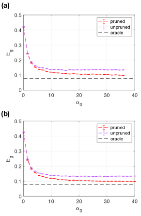
Figure 3: Comparison of the generalization error in simulations of a sparsely expanded two layer network before and after pruning the expanded units. (a) shows simulations for a student network with expansion factor $\beta=5$ and (b) shows simulations for a student network with $\beta=10$. We see for both values of $\beta$ the student network with the best overall performance is the network with sparse expansion with expanded weights are pruned after learning. The parameters $f=0.02$, $A=0.2$, $\sigma_{out}=0.25$, and $N_{0}=100$ and $200$ trials are used in both figures.

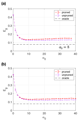
Figure 4: Comparison of the generalization error from simulations of a densely expanded two layer network before and after pruning the expanded units. (a) shows simulations for a student network with expansion factor $\beta=5$ and (b) shows simulations for a student network with $\beta=10$. We see that the densely expanded network performs best when the expanded weights are unpruned. However, the performance of the sparsely expanded network with pruned weights in 3 is superior to the densely expanded network regardless of whether the weights are pruned or kept. The parameters $f=0.5$, $A=0.2$, $\sigma_{out}=0.25$, and $N_{0}=100$ and $200$ trials were used for all figures.

The network represented in Eqns. 5 and 6 is difficult to study analytically because of correlations in the activities of the hidden layer induced by $J$ Babadi and Sompolinsky (2014). We therefore consider in the following section a simplified expansion scheme which we call, a stochastic architecture, and is shown in Fig. 1 D. In contrast to the deterministic scheme of Fig. 1 C, the activity patterns of the additional neurons in this architecture are not generated through connections from the input layer. Instead they are randomly generated for each training pattern, $\mu$, independent of $x_{\mu}$. The advantage of this scheme is that the random activities of the hidden neurons are statistically independent of each other and additionally for different training patterns, rendering the model amenable to study using the tools of statistical mechanics. Although this scheme is artificial from a biological perspective, we will show that when the deterministic layer is very sparse the system’s behavior is similar to the stochastic model.

III Theory of perceptron learning with expanded stochastic units

In this section, we develop intuition for the effect of sparse expansion on the generalization performance of a perceptron by considering a simpler single layer student network which can be solved analytically in the mean field limit. This network (shown in B of Fig. 1) is trained using data with $\mu=1,...,P$ binary labels $y^{\mu}$, generated by the noisy teacher network in Eqn. 1. For convenience, we keep the same normalization for the student and teacher weight vectors which corresponds to setting $\sigma_{w}^{2}=\beta$ in 1. The activity of the student network takes the form:

$$h=\frac{1}{\sqrt{N}}\left(\sum_{i=1}^{N_{0}}{w_{i}x_{i}}+\sum_{j=1}^{N_{+}}{\tilde{w}_{j}\tilde{x}_{j}}\right)$$ (10)

where $\tilde{x}_{j}^{\mu}$ are random units added to the input layer and are drawn iid from a gaussian distribution with zero mean and variance $\sigma_{in}^{2}$. The label $y$ given to input $x$ by the student is $y(x)=\text{sign}(h)$. The student weights are trained to yield the max margin solution in Eqn. 9.

III.1 Mean field theory

We now analyze the performance of the expanded student network in 10. We will denote the measurement density of the training set relative to the width of this student as $\alpha=\alpha_{0}/\beta$. The mean field theory below is exact in the thermodynamic limit, where $P,N\rightarrow\infty$ and $\alpha\sim O(1)$ .

To perform an ensemble average of the system’s properties over different realizations of training sets, we use the replica trick in a manner similar to Gardner (1987); Gardner and Derrida (1988); Gardner (1988); Seung et al. (1992); Watkin et al. (1993); Engel and Van den Broeck (2001). Full details of the replica calculation and the form of the saddle equations are given in Appendix A. We start by considering the version space for $n$ replicated students indexed by $a$:

$$\langle V^{n}\rangle = \int\prod_{a}{dw^{a}d\tilde{w}^{a}\delta\left(\sum_{i=1}^{N_{0}}(w_{i}^{a})^{2}+\sum_{j=1}^{N_{+}}(\tilde{w}_{j}^{a})^{2}-N\right)}$$ (11)

$$\times \prod_{\mu=1}^{P}\sum_{\sigma=\pm 1}\left\langle\Theta\left(\left[\sigma h^{\mu a}-\kappa\right]\right)\Theta(\sigma h_{0}^{\mu})\right\rangle$$

where we have normalized the weights so that $\|w^{a}\|^{2}+\|\widetilde{w}^{a}\|^{2}=N$ in all replicas, and $\Theta$ is the Heavyside step function. The quantities $h^{\mu a}$ are the student’s fields induced by the $\mu$ -th input and weight vector $(w^{a},\tilde{w}^{a})$ of the $a$-th replica; $h_{0}^{\mu}$ are the teacher fields induced by the $\mu$-th input including noise. The angular brackets denote averaging with respect to the gaussian input vectors, $x_{\mu}$(with variance $1)$, student input noise vector,$\tilde{x}_{\mu}$ (with variance $\sigma_{in}^{2}$) , teacher label noise, $\epsilon_{\mu}$ (with variance $\sigma_{out}^{2}$). Since the distribution of inputs is isotropic, one does not need to average over the teacher distribution. Evaluating Eqn. 11, we derive a mean field theory in terms of the order parameters $m_{a}$, $\tilde{r}_{a}$, $q_{ab}$ and $\tilde{q}_{ab}$ defined as

$$m_{a} =\frac{1}{N}\sum_{i=1}^{N_{0}}w_{i}^{0}w_{i}^{a}$$ (12)

$$\tilde{r}_{a} =\frac{1}{N}\sum_{i=1}^{N_{+}}(\tilde{w}_{i}^{a})^{2}$$ (13)

$$q_{ab} =\frac{1}{N}\sum_{i=1}^{N_{0}}w_{i}^{a}w_{i}^{b}$$ (14)

$$\tilde{q}_{ab} =\frac{\sigma_{in}^{2}}{N}\sum_{i=1}^{N_{0}}\tilde{w}_{i}^{a}\tilde{w}_{i}^{b}$$ (15)

The order parameters can be understood intuitively as follows: $m_{a}$ corresponds to the overlap between the student weights $w^{a}$ and the teacher perceptron weights. $\tilde{r}_{a}$ corresponds the norm of expanded weights $\tilde{w}^{a}$ ; $q_{ab}$ measures the overlap between student weight $w^{a}$ in replica and $w^{b}$ in replica $b$. Similary $\tilde{q}_{ab}$ measures the overlap of expansion weights $\tilde{w}^{a}$ and $\tilde{w}^{b}$ (scaled with the expansion-input variance $\sigma_{in}^{2}$).

We apply the replica symmetric (RS) ansatz for the order parameters $m_{a}$, $\tilde{r}_{a}$, $q_{ab}$, and $\tilde{q}_{ab}$, which is exact because the version space of weight vectors is connected. This allows us write the order parameter matrices in terms of the four scalar order parameters $m,\tilde{r},q,$ and $\tilde{q}$ as follows

$$m_{a} =m,$$ (16)

$$\tilde{r}_{a} =\tilde{r},$$ (17)

$$q_{ab} =(1-q-\tilde{r})\delta_{ab}+q,$$ (18)

$$\tilde{q}_{ab} =\left(\sigma_{in}^{2}\tilde{r}-\tilde{q}\right)\delta_{ab}+\tilde{q}$$ (19)

In the mean field limit, we can decompose $\left\langle V^{n}\right\rangle$ into the sum of an entropic term and energetic term which are both functions of $m,\tilde{r},q,$ and $\tilde{q}$

$$\left\langle V^{n}\right\rangle=\exp\left[nN(G_{0}(q,\tilde{q},\tilde{r},m)+\alpha G_{1}(q,\tilde{q},\tilde{r},m))\right]$$ (20)

Within the replica framework, the max-margin solution is the unique solution which maximizes the margin and corresponds to the equivalence of $w$ in all student replicas such that the overlaps $q\rightarrow 1-\tilde{r}$ and $\tilde{q}\rightarrow\sigma_{in}^{2}\tilde{r}$. Taking the limit $n\rightarrow 0$, the averaged free energy takes the following functional form

$$\langle\log V\rangle = N(G_{0}(\tilde{r},m)+\alpha G_{1}(\tilde{r},m))$$ (21)

We obtain three closed saddle point equations for $\kappa$, $m$, and $\tilde{r}$ by minimizing the free energy in Eqn. 21 with respect to $m$ and $\tilde{r}$ and requiring that $V\rightarrow 0$. The capacity of the network is determined by solving the mean field equations in the limit $\kappa\rightarrow 0$.

The performance of the system depends on the expansion parameter $\beta$, and the input and output noise variances $\sigma_{in}^{2}$ and $\sigma_{out}^{2}$. We will focus primarily on the case $\sigma_{in}=1$, where the mean field equations simplify considerably, and solve them for $\tilde{r}$ as a function of $m$ and $\beta$. We find that in this case the capacity of the network as defined in terms of $\alpha_{0}$ obeys the simple scaling relation

$$\alpha_{c}(\beta,\sigma_{out})=\beta\alpha_{c}(1,\sigma_{out})$$ (22)

where $\alpha_{c}(1,\sigma_{out})$ is the capacity of the unexpanded network shown in Fig. 5. We derive an expression for $E_{g}$ in terms of the mean field order parameters in Appendix D.

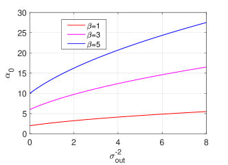
Figure 5: The network capacity for random inputs as a function inverse variance of the label noise obtained from the solution of the mean field equations for $\sigma_{in}=1$.

With the removal of the expanded weights $E_{g}$ takes the form:

$$E_{g} = \frac{1}{\pi}\left(\frac{\pi}{2}-\tan^{-1}\left(\frac{R}{\sqrt{1+\sigma_{out}^{2}-R^{2}}}\right)\right)$$ (23)

where $R$ is defined as the cosine of the angle between student and teacher weights which can be expressed in terms of the order parameter $m$ and $\tilde{r}$ as

$$R = \frac{m}{\sqrt{1-\tilde{r}}}$$ (24)

where the factor of $\sqrt{1-\tilde{r}}$ in Eqn. 24 is the fraction of the student weight norm in the subspace of the teacher. For student networks that are the same size as the teacher, $\tilde{r}=0$ and $R=m$. The generalization error for a student network that retains its expanded units after learning, with stochastic noise included in each test example, is given by replacing $R$ with $m$ in Eqn. 23. This is because the overlap $m$ is equivalent to cosine of the angle between teacher and student in the full network given the $\sqrt{N}$ normalization of both the teacher and expanded student. Thus, we see that for improved generalization performance, it is necessary to prune the augmented units after learning as was shown numerically for the deterministic network, Fig. 3. In the stochastic expansion, the intuition for removing these weights is straightforward as retaining them implies injecting stochastic activities in test example, uncorrelated with the task’s input, which will obviously reduce performance. The situation is different in the deterministic network in which correlations between the expanded and original components of the network the network are induced by the random map $J$, hence through learning $\tilde{w}$ acquire some information about the task. Indeed, as we have shown above, for dense expansion, retaining these weights slightly increases the performance. However, for sparse expansion, the correlation between the expanded activations and the task input is small (see below) hence pruning improves the performance similar to the stochastic case. Finally, we note that in the case of zero output noise, $E_{g}$ is just the angle between the student and teacher normalized by $\pi$ and the minimal error is given by Eqn. 23 with $R=1$, in agreement with Eqn. 4.

In Fig. 6, we plot the theoretical results for $E_{g}$ as a function of $\alpha_{0}$ for different values of $\beta$ for two values of $\sigma_{out}$ . For both high and low $\sigma_{out}$ , the generalization error decreases monotonically as a function of $\alpha_{0}$ for fixed $\beta$ and as a function of $\beta$ for fixed $\alpha_{0}$ . In LABEL:fig:thryaabeta and LABEL:fig:thryabbeta of Fig. 6 we show the minimal $E_{g}$ as a function of $\beta$ defined as the generalization error reached for each $\beta$ after minimizing over $\alpha_{0}$. An interesting question is whether for a given size of training set, there is a finite optimal expansion ratio. We find two qualitatively different behaviors dependent on the value of $\sigma_{out}$. For low values of $\sigma_{out}$, for a each fixed value of $\alpha_{0}$, the student network with the lowest generalization error is the smallest network which can fit all of the training examples. For higher values of $\sigma_{out}$, we find that making the network larger always improves the generalization performance for any value of $\alpha_{0}$, with the best performance occuring in the limit $\beta\rightarrow\infty$. The crossover between these two regimes occurs roughly around $\sigma_{out}\sim 0.5$. We conclude that adding noisy units during learning gives the network the capacity to fit the label noise and train on more examples in a way that does not interfere with the relevant weight information. This allows networks with larger expansion ratios to achieve better generalization as they are trained on more examples.

Figure 6: The replica theory results for the generalization error. $E_{g}$ is shown as a function of $\alpha_{0}$ for several values of the expansion factor $\beta$ for label noise with standard deviation $\sigma_{out}=0.25$ in (a) and standard deviation $\sigma_{out}=1$ in (b) . $E_{g}$ is shown as a function of $\beta$ for $\sigma_{out}=0.25$ in (a) and $\sigma_{out}=1$ in (b). $\sigma_{in}=1$ for all figures.

So far, we have considered the simple case of $\sigma_{in}=1$. We now discuss briefly the effect of varying $\sigma_{in}$. In Fig. 7, we demonstrate how varying the level of input noise can improve generalization error by comparing theory and simulations for different choices of $\sigma_{in}$. We find that calculations of $E_{g}$ from simulations match very well with the value obtained from solution of the mean field equations shown in Fig. 7. For low label noise, the generalization performance is most substantially improved when the variance of activity in the added units is much lower than the variance of patterns being learned, i.e. $\sigma_{in}<1$. In the deterministic network, this corresponds to choosing a small value for $A$. For fixed value of label noise $\sigma_{out}$, we find that there us an optimal variance $\sigma_{in}$ of the augmented units which minimizes $E_{g}$ for fixed measurement density $\alpha_{0}$ and expansion factor $\beta$. This value can be determined from the replica equations shown in Fig. 7 (b) and discussed in Appendix F. We will return to this issue in the Section C.

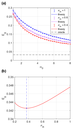
Figure 7: The replica theory results compared with simulations for the generalization error $E_{g}$. (a) shows $E_{g}$ for $\sigma_{out}=0.1$, $\beta=5$ and several values of $\sigma_{in}$. The error bars are computed from the mean and standard deviation of $400$ trials with $N_{0}=100.$ (b) shows $E_{g}$ v. $\sigma_{in}$ with $\alpha_{0}=3$, $\beta=5$, and $\sigma_{out}=1$, $\beta=5$ and the line represents the replica predictions for the value of $\sigma_{in}$ that minimize the generalization error.

III.2 Comparison between stochastic expansion and deterministic sparse expansion

Figure 8: Comparison of student networks with stochastic and sparse expansions. (a) compares simulations of the two layer student network with the theory results for the one layer network for $\beta=5$ for $\sigma_{out}=0.25$, $N_{0}=100$, and $200$ trials. In general, we see that student networks with stochastic added units attain superior performance when compared to a deterministic networks of the same size. (b) compares $E_{g}(\beta)$ for the case of stochastic augmented input units and deterministic hidden units with dense and sparse activity with $\sigma_{out}=0.5$, and $N_{0}=80$ . The parameters $\sigma_{in}=A=1$ and $200$ trials are used for both figures.

For networks expanded with sparse hidden layers, the parameter $A$ is closely related to $\sigma_{in}$. We directly compare the generalization performance of the student network with a sparse hidden layer (Eqn. 5) with the student network with stochastic units added to the input (Eqn. 10) by setting $\sigma_{in}=A$ so that the statistics of the expansion units match in the two networks. For simplicity we consider the case $\sigma_{in}=A=1$. Fig. 8 (a) shows the generalization error for each network with $\beta=5$ and Fig. 8 (b) shows the the generalization error as a function of the network expansion factor $\beta$. The stochastically expanded network achieves superior generalization performances for larger values of $\alpha_{0}$ and has a higher capacity. However, as can be seen, the performance of the deterministic networks approach that of the stochastic network upon increasing sparsity of the hidden layer activity. This is expected as the correlation in the sparse activities are weak and hence approach the uncorrelated stochastic limit.

III.3 Correspondence with slack regularization

While it is clear that expanding a network increases its capacity, it is not obvious that the expansion we have implemented should lead to improved generalization. While widening a network increases its capacity to fit more training data, it may also increase its Rademacher complexity improving its ability to learn random input output data Mohri et al. (2012). However, it turns out that the improved generalization performance in the networks we have studied can be related to an equivalence between our expanded network trained in the realizable regime and an unexpanded network trained in the unrealizable regime using slack regularization Hastie et al. (2004); Cristianini and Shawe-Taylor (2000), which we now explain.

We consider the relation between our expansion schemes for learning and that of slack SVM which is defined as,

$$\min_{w,\xi}\sum_{i=1}^{N_{0}}w_{i}^{2}+C\sum_{\mu=1}^{P}\xi^{\mu 2}\enspace s.t.\enspace\enspace y_{0}^{\mu}\left(\sum_{i=1}^{N_{0}}w_{i}x_{i}^{\mu}\right)\geq 1-\xi^{\mu}$$ (25)

While the SVM learning works only in the realizable regime, slack SVM is a convex optimization that allows non zero classification errors (when $\xi^{\mu}>1$) and regularizes them through the slack parameter $C$ that applies $L_{2}$ regularization of the slack variables $\xi^{\mu}$ . Although it does not minimize the training error, and its cost function does not have a well defined interpretation in terms of the classification tasks, it is a popular learning algorithm due to its simplicity and its empirically nice generalization properties .

To see the relation between slack parameters and the SVM with the stochastic expansion, we first note that the minimal $\tilde{w}$ of Eqn. 8 will necessarily be in the span of the $P$ input stochastic vectors, $\tilde{X}_{\mu}=\widetilde{x}^{\mu}y_{0}^{\mu}$ , since any projection on the null space will increase the norm of $\tilde{w}$ without contributing to the satisfaction of the inequalities. Defining new variable $\xi^{\mu}$ as

$$\xi^{\mu} = \tilde{X}^{\mu T}\tilde{w}$$ (26)

we can write the optimal $\tilde{w}$ as

$$\tilde{w}=(\tilde{X}^{T})^{+}\xi$$ (27)

where $\tilde{X}$is the matrix of input stochastic vectors and $+$ denotes the pseudo-inverse operation. Substituting Eqn. 27 into Eqn. 8 yields

$$\min_{w,\xi}\sum_{i=1}^{N_{0}}w_{i}^{2}+\sum_{\mu=1}^{P}\sum_{\nu=1}^{P}\xi^{\mu}C_{\mu\nu}\xi^{\nu}\enspace\enspace s.t.\enspace\enspace y_{0}^{\mu}\left(\sum_{i=1}^{N_{0}}w_{i}x_{i}^{\mu}\right)\geq 1-\xi^{\mu}$$ (28)

where $C=\tilde{(X}^{T}\tilde{X})^{+}$ or equivalently,

$$C_{\mu\nu}=\tilde{x}^{\mu}\tilde{x}^{\nu T}$$ (29)

which is just the sample covariance matrix of the expanded inputs in the training set. We recognize the second term in Eqn. 28 as the square of the Mahalanobis distance between the vector $\xi^{\mu}$ and a set of observations with zero mean and covariance matrix $C_{\mu\nu}$ . Thus, SVM with expanded networks is equivalent to slack SVM of the original network with a slack SVM that incorporates a Mahalanobis distance regularization of the slack variables with a covariance regularizer matrix $C$ injected by the expanded activities.

Furthermore, we can establish exact correspondence between the stochastic expansion and the slack SVM, Eqn. 28 in the limit large $\beta$ (and fixed $\alpha_{0}$) by noting that in this limit, $\widetilde{x}^{\mu}\widetilde{x}^{\nu T}\sim\delta^{\mu\nu}$, hence, the slack term becomes

$$\sum_{\mu=1}^{P}\sum_{\nu=1}^{P}\xi^{\mu}\langle C_{\mu\nu}^{-1}\rangle\xi^{\nu}\rightarrow\frac{1}{\sigma_{in}^{2}}\sum_{\mu=1}^{P}(\xi^{\mu})^{2}$$ (30)

which is a generic slack regularization term, with slack tradeoff parameter $\sigma_{in}^{-2}$. This implies that the addition of stochastic units becomes equivalent to the addition of slack terms in the limit $\beta\rightarrow\infty$. The equivalence breaks down for $N_{+}<P$ when the matrix $C_{\mu\nu}$ becomes uninvertible.

The above equivalence hold also for deterministic expansion, where now $C_{\mu\nu}=z^{\mu}z^{\nu T}$, see Eqn. 6. In the case of a sparse expansion, $C_{\mu\nu}$ has small off-diagonal elements and diagonal elements equaling $A$ which plays the role of the slack regularizer.

IV Extensions

So far, we have focused on a perceptron learning a noisy perceptron rule using convex learning algorithms. In the following section, we investigate whether random expansion of the network during learning is beneficial when the teacher is a given by nonlinear classification rule, and also in training with gradient based methods.

IV.1 Learning a nonlinear classification rule

Figure 9: Comparison of $E_{g}$ as a function of $\alpha_{0}$ for a student learning a quadratic teacher v. the same student learning a linear teacher with label noise. Error bars in (a) are obtained from simulations of a stochastic expanded student with $\sigma_{in}=1$ learning a quadratic teacher for $200$ trials and the solid lines correspond to the replica theory result for student learning from a noisy teacher. In (b) we compare simulations of a two layer student network with $f=0.02$ and $A=1$ learning from a quadratic teacher with simulations of the same student network learning from a noisy teacher for $400$ trials. The parameters $a=0.5$, $\sigma_{out}=1$, and $N_{0}=100$ are used in both figures.

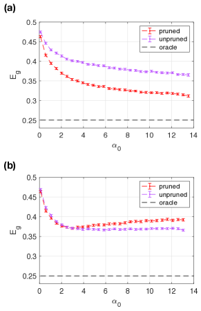
Figure 10: Simulation results for a two layer expanded student learning a quadratic teacher. (a) compares $E_{g}$ as a function of $\alpha_{0}$ before and after pruning for a sparse hidden layer with $f=0.02$ and (b) compares the performance before and after pruning for a dense hidden layer with $f=0.5$. The parameters $a=0.5$, $\sigma_{out}=1$, $\beta=10$, $N_{0}=100$ and $400$ trials are used in both figures

We model a perceptron learning a complex but deterministic rule by considering a student perceptron learning from a quadratic teacher. The target rule is then given by

$$y(x)=\text{sign}\left[a\frac{1}{\sqrt{N_{0}}}\sum_{i=1}^{N_{0}}{w_{i}^{0}x_{i}}+(1-a)\frac{1}{N_{0}}\sum_{i,j=1}{w_{ij}^{0}x_{i}x_{j}}\right]$$ (31)

with weights drawn iid as $w_{i}^{0},w_{ij}^{0}\sim\mathcal{N}(0,1)$. Here $a$ is a scalar coefficient between zero and one and denotes the relative weight of the linear component of the teacher. Clearly, a perceptron student cannot emulate perfectly such a rule. For a perceptron with $N_{0}$ weights, the optimal weights are $w=w^{0}$ with a non-zero minimal generalization error, $E_{\text{min}}$ which decreases with $a$ . In addition, there is a critical capacity, $\alpha_{c}$ above which the training examples are unrealizable, where $\alpha_{c}$ increases with $a$ .

We now discuss the effect of adding the stochastic random layer as in Fig. 1D of size $N^{+}$ with $N_{0}+N^{+}=\beta N_{0}$. Clearly the capacity for learning with zero training error increases with $\beta$. We now ask whether this expansion is also beneficial for generalization and whether prunning the network after learning improves performance. We have simulated training in this network using as before, the max-margin algorithm. Results shown in Fig. 9, confirm that the expanded stochastic network performs better than the unexpanded one. Furthermore, the results are in excellent agreement with the behavior in the case of the noisy perceptron target rule, with noise variance given by

$$\sigma_{out}=\frac{1-a}{a}.$$ (32)

We show simulation results for the two layer network with dense and sparse deterministic expansions in Fig. 10.  As in the case of a noisy teacher, the optimal generalization performance occurs after the extra neurons and synapses are removed from the network for a sparse expansion. This effect persists for values of $\beta$ as large as $\beta=40$ for $N_{0}=60$. In the case of the two layer network, it is not entirely obvious that removing the extra synapses would improve performance, as this structure may be used to learn something about the quadratic part of the teacher. It is possible that there may be parameter regimes in which it is beneficial to keep the extra weights unpruned that we have been unable to reach due to computational limitations on $\beta$ and $N_{0}$. Despite these potential shortcomings, our findings for both student architectures demonstrate that the benefits of expanding a network can also occur in the setting where the rule being learned is more complicated than the model.

Finally, we suggest that our results should hold in general for a nonlinear SVM teachers with field $h_{0}$ taking the following form

$$h_{0}=w^{0}\cdot\Phi(x)+\epsilon$$ (33)

where $\Phi(x)$ is a transformation from $\mathbb{R}^{N_{0}}\rightarrow\mathbb{R}^{M_{0}}$ defined by $\Phi(x)=(\Phi_{1}(x),\dots,\Phi_{M_{0}}(x))$. Given a training set $(x^{\mu},y^{\mu}_{0})$, we can consider a student with labels given by

$$y=\text{sign}(w\cdot\Psi(x))$$ (34)

where $\Psi(x)$ is a transformation from $\mathbb{R}^{N}\rightarrow\mathbb{R}^{M}$ defined by $\Psi(x)=(\Psi_{1}(x),\dots,\Psi_{M}(x))$. The max margin solution for the student weight vector is then

$$w=\sum_{\mu=1}^{P}\alpha_{\mu}y^{\mu}_{0}\Psi(x^{\mu}+\tilde{x}^{\mu})$$ (35)

where the coefficients $\alpha^{\mu}$ are given by solving the optimization problem 8 with constraints given by 9. The student labels are now given by

$$y =\text{sign}\left(\sum_{\mu=1}^{P}\alpha_{\mu}y_{0}^{\mu}K(x^{\mu}+x,x+\tilde{x})\right)$$ (36)

where the kernel $K$ is defined as

$$K(x,y)=\Psi(x)\cdot\Psi(y)$$ (37)

If the student perceptron uses the same transformation $\Phi(x)$ as the teacher, expanding the dimensionality of the input $x$ produces the same improvement in generalization performance as shown in section III. This is because the training data is linearly separable without noise. We demonstrate this with simulations with $\Phi(x)$ chosen as the eigenfunction of a quadratic kernel with a stochastic expansion of the input shown in Fig.11. When the transformation $\Psi(x)$ is less complex than the transformation $\Phi(x)$ of the teacher, we expect that expanding the input of the student results in improved generalization qualitatively similar to our results for a linear student learning a quadratic teacher discussed in the beginning of the section. We also expect these results to hold for networks with sparse expansions.

Figure 11: Simulation results for a quadratic kernel student with stochastic expanded input layer learning a quadratic kernel teacher with label noise. The parameters $\sigma_{out}=1$, $N_{0}=20$ and $200$ trials are used in both figures.

IV.2 Logistic regression

We now consider alternative optimization methods and loss functions which allow a neural network to be trained beyond capacity. One example is logistic regression, with a cost function given by

$$L(w) = \sum_{\mu=1}^{P}\log\left(1+\exp(-u^{\mu})\right)$$ (38)

$$u^{\mu} = \frac{1}{\sqrt{N}}\sum_{i=1}^{N}y^{\mu}w_{i}x_{i}^{\mu}$$ (39)

In the following, we consider full batch gradient descent so that the update to the weights at each training epoch is given by

$$\Delta w_{i}= -\eta\frac{\partial L(w)}{\partial w_{i}}$$

In Soudry et al. (2018) it was shown that the normalized weight vector obtained by a minimizing the logistic regression loss function via gradient descent should converge to the max margin solution after a sufficiently long training time if the training data is linearly separable. However, this correspondence depends on learning parameters such as $\eta$ and the number of iterations. Note that in general, for convergence to the max margin solution one needs to run the logistic regression gradient based training for longer times than required for finding a solution with zero training error. For unrealizeable rules, e.g., the noisy teacher in Eqn. 1 and the quadratic teacher Eqn. 31, logistic regression and max-margin classification are not equivalent for large $P$ because the training set provided by the teacher is not linearly separable.

In previous sections we have shown that stochastic and sparse expansions of perceptron networks increase the capacity of a network by making the training set linearly separable in a higher dimensional space. Thus, it is natural to ask under what conditions training an expanded network via logistic regression will result in a weight vector that converges to the new max margin solution in the higher dimensional space and if this solution can yield a superior generalization performance compared to a gradient based training of the unexpanded student network.

We have simulated the logistic regression learning for the problem of learning a noisy perceptron teacher, for some values of $\eta$ and number of training epochs. We first consider the case $\beta=1$, i.e. a student the same size as the teacher. For $\alpha_{0}$ below capacity, the margin increases monotonically with training epochs and converges asymptotically to the maximum margin, as shown in Fig. 13 (b) ($\alpha_{0}=3$), with convergence time depending on $\eta$. In Fig. 13 (a) we show for the same $\alpha_{0}$ the value of the overlap between student and teacher, as a function of $\eta t$. Interestingly, while $R$ does seem to converge asymptotically to the maximum margin value, it is not monotonic and in fact reaches a maximum value larger than the infinite time asymptote early in the training. Thus, the max margin solution is not necessarily the one with the best generalization performance. Above capacity, logistic regression permits solutions with nonzero training error, and we find that it results with good generalization performance. The value of $R$ as a function of $\alpha_{0}$ is shown in Fig. 12. As seen, for small $\alpha_{0}$ the overlap (achieved after a large number of epochs) is close to the max margin solution with precise values dependent on $\eta$ and the stopping criterion. When $\alpha_{0}$ increases above capacity, $R$ increases monotonically and seems to approach $R=1$ for large $\alpha_{0}$ (corresponding to the optimal solution $w=w^{0}$), although the amount of increase depends on $\eta$. Note that in this regime both $R$ and $\kappa$ converge fast to their asymptotic values as shown in Fig. 13.

Figure 12: Simulation results for logistic regression showing $R$ v. $\alpha_{0}$ for various learning rates for $N=100$, and $\sigma_{out}=0.5$.

Figure 13: Simulation results for logistic regression with $\beta=1$ and $\sigma_{out}=0.5$ where $t$ is defined as the number of training epochs. (a) shows $R$ as a function of $\eta t$ where for $\alpha_{0}=3$ (below capacity) and $\alpha_{0}=8$ (above capacity) for $N=100$.(b) shows the margin $\kappa$ as a function of $\eta t$ for $\alpha_{0}=3$ and $\alpha_{0}=8$.

For an expanded student network i.e. $\beta>1,$ we find that $R$ converges to the max margin value after long training time for $\alpha_{0}$ below capacity as shown in Fig. 14 and continues to increase with $\alpha_{0}$ as it increases above capacity. However, for fixed values of $\eta$ that are not too large, the largest value of $R$ for any $\alpha_{0}$ is obtained for the unexpanded network, i.e., $\beta=1$ as shown in Fig. 14. This implies that in this range of parameters, expanding the network does not improve generalization performance.

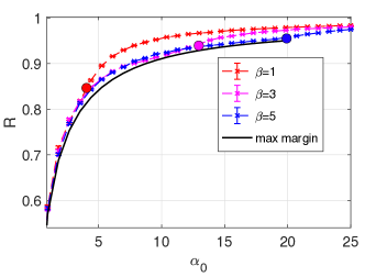
Figure 14: Simulation results for logistic regression for several values of $\beta$ with $N_{0}=100$ and $\sigma_{out}=0.5$ showing $R$ v. $\alpha_{0}$ for $\beta=1,3,5$ with fixed learning rate $\eta=0.01$. The max margin line in the plot corresponds to the max margin solution for $\beta=5$ and the circles mark the capacity for each value of $\beta$.

V Discussion

In this work, we have shown how expanding the architecture of neural networks can provide computational benefits beyond better expressivity and improve the generalization performance of the network after the expanded weights and neurons are pruned after training. We obtain equations for the order parameters characterizing generalization in randomly expanded perceptron networks (called stochastic expansion) in the mean limit and show explicitly that expansion allows for more accurate learning of noisy or complex teacher networks. This is achieved by increasing network capacity during training, allowing the learning to benefit from more examples. We show a qualitatively similar improved performance when expanding by adding fixed random weights (deterministic expansion) connecting the input to sparsely active hidden units. An additional insight into our results is provided by showing that the expansion is effectively similar to the addition of slack variables to the max-margin learning.

In our analysis, we considered training sets drawn iid from a Gaussian distribution with no spatial structure. It would be interesting to see how our results could be extended to learning structured data. In particular, Chung et al. (2018) developed a theory for the linear classification of manifolds with arbitrary geometry by using special anchor points on the manifolds to define novel geometrical measures of radius and dimension which can be directly linked to the classification capacity for manifolds of various geometries. It would be interesting to see if sparse expansions similar to those we have studied could be useful in classifying noisy manifolds and if there is any correspondence to SVMs containing anisotropic slack regularization encoded in the structure of the covariance matrix as in Eqn. 29.

It would also be interesting to determine how and if our observations apply to learning in deep networks with multiple layers. Neural network pruning techniques have been widely discussed in the deep learning community and it has been shown that neural network pruning techniques can reduce parameter counts of trained network by over 90% without compromising accuracy LeCun et al. (1990); Han et al. (2015). Training a pruned model from scratch is worse than retraining a pruned model, which suggests that the extra capacity of the network allows it to find more optimal solutions. In Frankle and Carbin (2019), the authors find that dense, randomly-initialized, feed-forward networks contain subnetworks that can reach test accuracy comparable to the original network in a similar number of training iterations when trained in isolation. It would be interesting to see if the extra weights in the larger networks can be translated into a regularization condition on the subnetwork.

Most of our work focused on max margin learning. We have explored the effect of expansion on gradient based learning with logistic regression cost function. We find that for appropriate choice of learning rate and learning time, generalization is similar to the max margin performance below the network capacity, consistent with Soudry et al. (2018). We also found that in the explored parameter range, optimal generalization performance is achieved by the unexpanded network, as gradient based learning can extract useful information even beyond the capacity learning. However, understanding the generalization performance in gradient based learning requires a more thorough understanding of the role of learning rate and training time is quite difficult given the lack of theory for the training dynamics for logistic regression. It would be interesting to see if there is a way to scale $\eta$ such that expanding the network can provide similar benefits for logistic regression beyond capacity as for max margin learning. We leave this to future work.

We also note that generalization can also improve when adding unquenched noise to the student labels during training with logistic loss as this prevents the classifier from overfitting (results not shown; Bishop (1995); Welling and Teh (2011)). This differs from our construction for two reasons. The first is that our student by construction learns the weights in the extended part of the network. The second is that our dimensionality expansion changes the properties of the training set in that a nonlinearly separable training set in the original space may become linearly separable in the higher dimensional expanded space.

VI Acknowledgments

We thank Haozhe Shan and Weishun Zhong for valuable discussions concerning our logistic regression results and Subir Sachdev for helpful comments on the draft. This work is partially supported by the Gatsby Charitable Foundation, the Swartz Foundation, and the National Institutes of Health (Grant No. 1U19NS104653). J.S. acknowledges support from the National Science Foundation Graduate Research Fellowship under Grant No. DGE1144152.

Appendix A Mean field equations

We outline the derivation of the mean field equations used to compute the order parameters defined in Eqns. 12,13, 14, and 15 which are used to compute the generalization error given in Eqn. 23. We define the student field for each replica of the student network as:

$$h^{\mu a}=\frac{1}{\sqrt{N}}\sum_{i=1}^{N}W_{i}X{}^{\mu}=\frac{1}{\sqrt{N}}\left(\sum_{i=1}^{N_{0}}w_{i}^{a}x_{i}^{\mu}+\sum_{j=1}^{N_{+}}\tilde{w}_{j}^{a}\tilde{x}_{j}^{\mu}\right),$$ (40)

and the teacher field as

$$h^{\mu 0}=\frac{1}{\sqrt{N}}\sum_{i=1}^{N}W_{i}^{0}\cdot X_{i}{}^{\mu}+\epsilon^{\mu}=\frac{1}{\sqrt{N}}\sum_{i=1}^{N_{0}}w_{i}^{0}x_{i}^{\mu}+\epsilon^{\mu}.$$ (41)

We can now write the average over the version space in Eqn. 20 in terms of these new variables

$$V^{n}=\left\langle\int\prod_{i=1}^{N_{0}}\prod_{j=1}^{N_{+}}\prod_{a}{dw_{i}^{a}d\tilde{w}_{j}^{a}\delta\left(\sum_{i=1}^{N_{0}}(w_{i}^{a})^{2}+\sum_{j=1}^{N_{+}}(\tilde{w}_{j}^{a})^{2}-N\right)}\prod_{\mu}^{P}\int dh^{\mu a}\int d\hat{h}^{\mu a}\int dh_{0}^{\mu}\int d\hat{h}_{0}^{\mu}\left[\sum_{\sigma}\Theta_{\mu,a}\left(yh^{\mu a}-\kappa\right)\Theta(yh_{0}^{\mu})\right]I\right\rangle$$ (42)

where $I$ is given by

$$I = \exp\left[-i\sum_{a\mu}h^{\mu a}\hat{h}^{\mu a}-i\sum_{\mu}h_{0}^{\mu}\hat{h}_{0}^{\mu}+i\sum_{a\mu}\hat{h}^{\mu a}\frac{1}{\sqrt{N}}\sum_{i=1}^{N}\left(W_{i}^{a}X_{i}^{\mu}\right)+i\sum_{\mu}\hat{h}_{0}^{\mu}\left(\frac{1}{\sqrt{N}}\sum_{i=1}^{N}W_{i}^{0}\cdot X_{i}^{\mu}+\epsilon^{\mu}\right)\right]$$ (43)

and the constraints in Eqns. 40 and 41 are implemented by the Lagrange multipliers $h^{\mu a}$ and $\hat{h}_{0}^{\mu}$. Averaging over the input $x^{\mu}$, $\tilde{x}$, and the noise $\epsilon^{\mu}$, $I$ becomes

$$I= \int\prod_{\mu=1}^{P}\prod_{i=1}^{N_{0}}\frac{dx_{i}^{\mu}}{\sqrt{2\pi}}e^{-\frac{(x^{\mu})^{2}}{2}}\prod_{j=1}^{N_{+}}\frac{d\tilde{x}_{j}^{\mu}}{\sqrt{2\pi\sigma_{in}^{2}}}e^{-\frac{(\tilde{x}^{\mu})^{2}}{2\sigma_{in}^{2}}}\frac{d\epsilon^{\mu}}{\sqrt{2\pi\sigma_{out}^{2}}}e^{-\frac{(\epsilon^{\mu})^{2}}{2\sigma_{out}^{2}}}$$

$$\times \exp\left[-i\sum_{\mu\alpha}h^{\mu a}\hat{h}^{\mu a}-i\sum_{\mu}h_{0}^{\mu}\hat{h}_{0}^{\mu}+i\sum_{\mu a}\sum_{i=1}^{N_{0}}\frac{1}{\sqrt{N}}(\hat{h}^{\mu a}w_{i}^{a}+\hat{h}_{0}^{\mu}w_{i}^{0})x_{i}^{\mu}+i\sum_{\mu a}\sum_{j=1}^{N_{+}}\frac{1}{\sqrt{N}}(\hat{h}^{\mu a}\tilde{w}_{j}^{a}\tilde{x_{j}}^{\mu})+i\sum_{\mu}\hat{h}_{0}^{\mu}\epsilon^{\mu}\right]$$

$$= \exp\left[-\sum_{\mu}\Big{(}i\sum_{a}h^{\mu a}\hat{h}^{\mu a}+ih_{0}^{\mu}\hat{h}_{0}^{\mu}+\sum_{a}\hat{h}^{\mu a}\hat{h}_{0}^{\mu}\sum_{i=1}^{N_{0}}\frac{w_{i}^{a}\cdot w_{i}^{0}}{N}+\frac{(1+\sigma_{out}^{2})}{2}\hat{h}_{0}^{\mu 2}+\frac{1}{2}\sum_{ab}\hat{h}^{\mu a}\hat{h}^{\mu b}\left(\sum_{i=1}^{N_{0}}\frac{w_{i}^{a}w_{i}^{b}}{N}+\sigma_{in}^{2}\sum_{j=1}^{N_{+}}\frac{\tilde{w}_{j}^{a}\tilde{w}_{j}^{b}}{N}\right)\Big{)}\right]$$ (44)

We define the order parameters $m_{a}$, $q_{ab}$ and $\tilde{q}_{ab}$ as

$$m_{a} =\frac{1}{N}\sum_{i=1}^{N_{0}}w_{i}^{0}w_{i}^{a}$$ (45)

$$q_{ab} =\frac{1}{N}\sum_{i=1}^{N_{0}}w_{i}^{a}w_{i}^{b}$$ (46)

$$\tilde{q}_{ab} =\frac{\sigma_{in}^{2}}{N}\sum_{j=1}^{N_{+}}\tilde{w}_{j}^{a}\tilde{w_{j}}^{b}$$ (47)

For further convenience, we write the sum of $q_{ab}$ and $\tilde{q}_{ab}$ as

$$Q_{ab}=q_{ab}+\tilde{q}_{ab}.$$ (48)

In terms of the order parameters, $I$ becomes

$$I = \exp\left[-\sum_{\mu}\Big{(}i\sum_{\alpha}h^{\mu a}\hat{h}^{\mu a}+ih^{\mu 0}\hat{h}^{\mu 0}+\sum_{a}\hat{h}^{\mu a}\hat{h}^{\mu 0}m_{a}+\frac{(1+\sigma_{out}^{2})}{2}(\hat{h}^{\mu 0})^{2}+\frac{1}{2}\sum_{ab}\hat{h}^{\mu a}\hat{h}^{\mu b}Q_{ab}\Big{)}\right]$$ (49)

We can now do the integrals over $\hat{h}$ and $\hat{h}_{0}$ which gives us

$$\prod_{\mu}^{P}\int dh^{\mu a}\int d\hat{h}^{\mu a}\int dh^{\mu 0}\int d\hat{h}^{\mu 0}I = \prod_{\mu}^{P}\int dh^{\mu a}\int D\bar{h}^{\mu 0}\det(Q_{ab}-\bar{m}^{2})^{-\frac{P}{2}}X$$ (50)

where we have defined $X$ as

$$X = \exp\left[-\frac{1}{2}\sum_{\mu}\sum_{ab}(\bar{h}^{\mu 0}\bar{m}-h^{\mu a})(Q_{ab}-\bar{m}^{2})^{-1}(\bar{h}^{\mu 0}\bar{m}-h^{\mu b})\right]$$ (51)

and $\bar{m}$ and $\bar{h}$ as

$$\bar{m} =\frac{m}{\sqrt{1+\sigma_{out}^{2}}}$$ (52)

$$\bar{h}^{0} =\frac{h^{0}}{\sqrt{1+\sigma_{out}^{2}}}$$ (53)

We now define the additional parameter $\tilde{r}_{a}$ as

$$\tilde{r}_{a} =\frac{1}{N}\sum_{i=1}^{N_{+}}(\tilde{w}_{i}^{a})^{2}$$ (54)

Since the solution space is connected, we can make the following replica symmetric ansatz for $m_{a}$, $q_{ab}$, $\tilde{q}_{ab}$, and $\tilde{r}_{a}$

$$m_{a} =m$$ (55)

$$\tilde{r}_{a} =\tilde{r}$$ (56)

$$q_{ab} =(1-\tilde{r}-q)\delta_{ab}+q$$ (57)

$$\tilde{q}_{ab} =\left(\sigma_{in}^{2}\tilde{r}-\tilde{q}\right)\delta_{ab}+\tilde{q}$$ (58)

$$Q_{ab} =(r_{Q}-Q)\delta_{ab}+Q$$ (59)

where $Q=q+\tilde{q}$ and $r_{Q}=1-(1-\sigma_{in}^{2})\tilde{r}$. The inverse of the matrix in Eqn. 51 is given by

$$(Q_{ab}-\bar{m}^{2})^{-1}=\frac{1}{r_{Q}-Q}\delta_{ab}-\frac{Q-\bar{m}^{2}}{(r_{Q}-Q)^{2}}$$ (60)

we now define $X^{\prime}$ as:

$$X^{\prime} = \prod_{\mu}^{P}\int dh^{\mu a}\int dh_{0}^{\mu}\exp\Big{[}-\frac{P}{2}\log\det(Q_{ab}-\bar{m}^{2})\Big{]}X^{P}$$ (61)

Plugging in the replica symmetric ansatz in Eqns. 55, 56, 57, 58, this becomes

$$X^{\prime} =\prod_{\mu}^{P}\int dh^{\mu a}\int dh^{\mu 0}\exp\Big{[}-\frac{1}{2(r_{Q}-Q)}\sum_{\mu a}(h^{\mu a})^{2}+\frac{1}{2}\frac{Q-\bar{m}^{2}}{(r_{Q}-Q)^{2}}\sum_{\mu}\left(\sum_{a}h^{\mu a}\right)^{2}$$

$$+\frac{1}{(r_{Q}-Q)}\sum_{\mu}\bar{h}^{\mu 0}\bar{m}\sum_{a}h^{\mu a}-\frac{n\sum_{\mu}(\bar{h}^{\mu 0}\bar{m})^{2}}{2(r_{Q}-Q)}-\frac{P}{2}\log\det(Q_{ab}-\bar{m}^{2})\Big{]}$$ (62)

We decouple terms with different replica indices in Eqn. 62 via a Hubbard-Stratonovich transformation by introducing the auxiliary variable $t$. Then $X^{\prime}$ becomes

$$X^{\prime} =2\int_{0}^{\infty}D\bar{h}_{0}\int Dt\left[\int_{\kappa}^{\infty}\frac{dh}{\sqrt{2\pi}}\exp\Big{(}-\frac{1}{2}\frac{h^{2}}{r_{Q}-Q}+\frac{\sqrt{Q-\bar{m}^{2}}}{r_{Q}-Q}ht+\frac{1}{r_{Q}-Q}h\bar{h}_{0}\bar{m}-\frac{\bar{m}^{2}\bar{h}_{0}^{2}}{2(r_{Q}-Q)}\Big{)}\right]^{n}$$ (63)

where $Dx=\frac{dx}{\sqrt{2\pi}}e^{-\frac{x^{2}}{2}}$.

Once we evaluate all of the integrals in the expression for $\langle V^{n}\rangle$ we can write it in the following form

$$\langle V^{n}\rangle=\exp(nN(G_{0}(q,\tilde{q},\tilde{r},m)+\alpha G_{1}(q,\tilde{q},\tilde{r},m)))$$ (64)

where $G_{0}(q,\tilde{q},m)$ is an entropic contribution coming from from the integral over the weights and $G_{1}(q,\tilde{q},\tilde{r},m)$ is an energetic contribution whose form is dictated by the learning rule.
We can start by computing the energetic contribution. We define $A(t,\bar{h}_{0})$ and $Z(t,\bar{h}_{0})$ as

$$A(t,\bar{h}_{0}) = \frac{1}{2(r_{Q}-Q)}\left(\sqrt{Q-\bar{m}^{2}}t+\bar{h}_{0}\bar{m}\right)^{2}-\frac{\bar{m}^{2}\bar{h}_{0}^{2}}{2(r_{Q}-Q)}$$ (65)

$$Z(t,\bar{h}_{0}) = \int_{\kappa}^{\infty}\frac{dh}{\sqrt{2\pi}}\exp\left(-\frac{1}{2(r_{Q}-Q)}\left[h-\left(\sqrt{Q-\bar{m}^{2}}t+\bar{h}_{0}\bar{m}\right)\right]^{2}\right)$$ (66)

and rewrite $X^{\prime}$ as

$$X^{\prime} = 2\int_{0}^{\infty}D\bar{h}_{0}\int Dt\Big{[}\exp(nA(t,\bar{h}_{0}))Z^{n}(t,\bar{h}_{0})\Big{]}$$ (67)

We define $A$ as the average over $t$, $\bar{h}^{0}$ of $A(t,\bar{h}_{0})$, i.e.

$$A = \int_{0}^{\infty}D\bar{h}^{0}\int DtA(t,\bar{h}_{0})=\frac{Q-\bar{m}^{2}}{2(r_{Q}-Q)}$$ (68)

In the limit $n\rightarrow 0$, $X^{\prime}$ becomes

$$X^{\prime}=\exp\left(An+2n\int_{0}^{\infty}D\bar{h}^{0}\int Dt\log Z(t,\bar{h}^{0})\right)$$ (69)

We can do the following shift of variables

$$x =\left(\sqrt{Q-\bar{m}^{2}}t+\bar{h}_{0}\bar{m}\right)/\sqrt{Q}$$ (70)

$$y =\left(-\bar{m}t+\sqrt{Q-\bar{m}^{2}}\bar{h}_{0}\right)/\sqrt{Q}$$ (71)

which allows us to write $t$ and $\bar{h}^{0}$ as

$$t =\left(\sqrt{Q-\bar{m}^{2}}x-y\bar{m}\right)/\sqrt{Q}$$ (72)

$$\bar{h}_{0} =\left(x\bar{m}+\sqrt{Q-\bar{m}^{2}}y\right)/\sqrt{Q}$$ (73)

and $Z(t,\bar{h}_{0})$ as

$$Z(x) = \int_{\kappa}^{\infty}\frac{dh}{\sqrt{2\pi}}\exp\left(-\frac{(h-\sqrt{Q}x)^{2}}{2(r_{Q}-Q)}\right)=\sqrt{r_{Q}-Q}H\left(\frac{\kappa-\sqrt{Q}x}{\sqrt{r_{Q}-Q}}\right)$$ (74)

Under this transformation, the Gaussian integrals become

$$\int_{0}^{\infty}D\bar{h}^{0}\int Dt=\int Dx\int_{-x\bar{m}/\sqrt{Q-\bar{m}^{2}}}^{\infty}Dy=\int DxH\left(-x\bar{m}/\sqrt{Q-\bar{m}^{2}}\right)$$ (75)

where we define

$$H(x) = \int_{x}^{\infty}Dy$$ (76)

This gives us

$$2\int_{0}^{\infty}Dh^{0}\int Dt\log Z(t,h^{0})= 2\int DxH\left(-x\bar{m}/\sqrt{Q-\bar{m}^{2}}\right)\log Z(x)$$ (77)

$$= 2\int DxH\left(-x\bar{m}/\sqrt{Q-\bar{m}^{2}}\right)\log H\left(\frac{\kappa-\sqrt{Q}x}{\sqrt{r_{Q}-Q}}\right)+\frac{1}{2}\log(r_{Q}-Q)$$

So $X^{\prime}$ becomes

$$X^{\prime} = \exp\left(2\int DxH\left(-x\bar{m}/\sqrt{Q-\bar{m}^{2}}\right)\log H\left(\frac{\kappa-\sqrt{Q}x}{\sqrt{r_{Q}-Q}}\right)+\frac{1}{2}\log(r_{Q}-Q)+A\right)^{n}$$ (78)

Using the relation

$$A-\frac{1}{2n}\text{log}\text{det}(Q_{ab}-\bar{m}^{2})+\frac{1}{2}\log(r_{Q}-Q) = 0$$ (79)

the replicated volume of the version space become

$$\langle V^{n}\rangle =\int\prod_{a=1}^{n}d^{N_{0}}w^{a}d^{N_{1}}\tilde{w^{a}}\delta\left(\sum_{i=1}^{N_{0}}(w_{i}^{a})^{2}+\sum_{j=1}^{N_{+}}(\tilde{w}_{j}^{a})^{2}-N\right)\int dm\int dq_{ab}\int d\tilde{q}_{ab}\delta(Nm-\sum_{i=1}^{N_{0}}w_{i}^{a}w_{i}^{0})$$

$$\prod_{ab}\delta\left(Nq_{ab}-\sum_{i=1}^{N_{0}}w_{i}^{a}w_{i}^{b}\right)\delta\left(N\tilde{q}_{ab}-\sigma_{in}^{2}\sum_{j=1}^{N_{+}}\tilde{w}_{j}^{a}\tilde{w}_{j}^{b}\right)\exp\Big{(}2n\int DxH\left(-\frac{x\bar{m}}{\sqrt{Q-\bar{m}^{2}}}\right)\log H\left(\frac{\kappa-\sqrt{Q}x}{\sqrt{r_{Q}-Q}}\right)\Big{)}^{P}$$

We can compute the entropic term $G_{0}(q,\tilde{q},m,\tilde{r})$ by considering the integrals over configurations of weights allowed by the delta functions. Then $\exp(nN(G_{0}(q,\tilde{q},\tilde{r},m))$ is given by

$$\exp(nN(G_{0}(q,\tilde{q},\tilde{r},m)) = \int\prod_{a=1}^{n}\int dw_{a}d\tilde{w}_{a}\delta\left(Nm-\sum_{i=1}^{N_{0}}w_{i}^{a}w_{i}^{0}\right)$$

$$\times \prod_{ab}\delta\left(Nq_{ab}-\sum_{i=1}^{N_{0}}w_{i}^{a}w_{i}^{b}\right)\delta\left(N\tilde{q}_{ab}-\sigma_{in}^{2}\sum_{j=1}^{N_{+}}\tilde{w}_{j}^{a}\tilde{w}_{j}^{b}\right)$$

Introducing the Lagrange multipliers $\hat{m}$, $\hat{q}_{ab}$, and $\hat{\tilde{q}}_{ab}$, Eqn. A can be written as

$$\exp(nN(G_{0}(q,\tilde{q},\tilde{r},m)) =\int\prod_{a=1}^{n}dw^{a}d\tilde{w}^{a}\int\frac{d\hat{m}}{\sqrt{2\pi}}\int\frac{d\hat{q}_{ab}}{\sqrt{4\pi}}\int\frac{d\hat{\tilde{q}}_{ab}}{\sqrt{4\pi}}\exp\Big{(}\frac{i}{2}\sum_{ab}\hat{q}_{ab}\left(Nq_{ab}-\sum_{i=1}^{N_{0}}w_{i}^{a}w_{i}^{b}\right)$$

$$+\frac{i}{2}\sum_{ab}\hat{\tilde{q}}_{ab}\left(N\tilde{q}_{ab}-\sigma_{in}^{2}\sum_{j=1}^{N_{+}}\tilde{w}_{j}^{a}\tilde{w}_{j}^{b}\right)+i\sum_{a}\hat{m}_{a}\left(Nm_{a}-\sum_{i=1}^{N_{0}}w_{i}^{a}w_{i}^{0}\right)\Big{)}$$

$$=\int\frac{d\hat{m}}{\sqrt{2\pi}}\int\frac{d\hat{q}_{ab}}{\sqrt{4\pi}}\int\frac{d\hat{\tilde{q}}_{ab}}{\sqrt{4\pi}}\exp\left(\frac{iN}{2}\sum_{ab}\hat{q}_{ab}q_{ab}+\frac{iN}{2}\sum_{ab}\hat{\tilde{q}}_{ab}\tilde{q}_{ab}+iN\sum_{a}\hat{m}_{a}m_{a}\right)$$

$$\times\int\prod_{a=1}^{n}dw^{a}d\tilde{w}^{a}\exp\left(-iH(w^{a},\tilde{w^{a}},w^{0})\right)$$ (82)

where we have defined a “Hamiltonian” $H(w_{a},\tilde{w}_{a},w_{0})$ as

$$H(w^{a},\tilde{w}^{a},w^{0}) = \frac{1}{2}\sum_{ab}(\hat{q}_{ab}\sum_{i=1}^{N_{0}}w_{i}^{a}w_{i}^{b}+\sigma_{in}^{2}\hat{\tilde{q}}_{ab}\sum_{j=1}^{N_{+}}\tilde{w}_{j}^{a}\tilde{w}_{j}^{b})+\sum_{a}\sum_{i=1}^{N_{0}}{w_{i}^{a}w_{i}^{0}\hat{m}_{a}}$$ (83)

Doing a Wick rotation $i\hat{m}_{a}\rightarrow\hat{m}_{a}$, $i\hat{q}_{ab}\rightarrow\hat{q}_{ab}$, $i\hat{\tilde{q}}_{ab}\rightarrow\hat{\tilde{q}}_{ab}$ and integrating over the weights $\bm{w}$ and $\tilde{\bm{w}}$, we have

$$\exp(nN(G_{0}(q,\tilde{q},\tilde{r},m) =\int\frac{d\hat{m}}{\sqrt{2\pi}}\int\frac{d\hat{q}_{ab}}{\sqrt{4\pi}}\int\frac{d\hat{\tilde{q}}_{ab}}{\sqrt{4\pi}}\exp\left(\frac{N}{2}\sum_{ab}\hat{q}_{ab}q_{ab}+\frac{N}{2}\sum_{ab}\hat{\tilde{q}}_{ab}\tilde{q}_{ab}+N\sum_{a}\hat{m}_{a}m\right)$$

$$\times\int\prod_{a=1}^{n}dw^{a}d\tilde{w}^{a}\exp\left(-\frac{1}{2}\sum_{ab}(\hat{q}_{ab}\sum_{i=1}^{N_{0}}w_{i}^{a}w_{i}^{b}+\sigma_{in}^{2}\hat{\tilde{q}}_{ab}\sum_{j=1}^{N_{+}}\tilde{w}_{j}^{a}\tilde{w}_{j}^{b})-\sum_{\alpha}{\sum_{i=1}^{N_{0}}w_{i}^{a}w_{i}^{0}\hat{m}_{a}})\right)$$

$$=\int\frac{d\hat{m}}{\sqrt{2\pi}}\int\frac{d\hat{q}_{ab}}{\sqrt{4\pi}}\int\frac{d\hat{\tilde{q}}_{ab}}{\sqrt{4\pi}}\exp\left(\frac{N}{2}\sum_{ab}\hat{q}_{ab}q_{ab}+\frac{N}{2}\sum_{ab}\hat{\tilde{q}}_{ab}\tilde{q}_{ab}+N\sum_{a}\hat{m}_{a}m\right)$$

$$\times\exp\left(\frac{N}{2}\sum_{ab}\hat{m}_{a}\hat{q}_{ab}^{-1}\hat{m}_{b}-\frac{N\beta^{-1}}{2}\log\det\hat{q}-\frac{N(1-\beta^{-1})}{2}\log\det\hat{\tilde{q}}\sigma_{in}^{2}\right)$$ (84)

We can evaluate the integral on the saddle point by solving for $\hat{m}_{a}$, $\hat{q}_{ab}$ ,and $\hat{\tilde{q}}_{ab}$ using the three saddle point equations

$$0 =\frac{N}{2}m_{\gamma}+\frac{N}{2}\sum_{b}(\hat{q}_{cb}^{-1})\hat{m}_{b}$$ (85)

$$0 =-\frac{N}{2}\sum_{ab}\hat{m}_{a}(\hat{q}_{ac})^{-1}(\hat{q}_{bd})^{-1}\hat{m}_{b}-\frac{N\beta^{-1}}{2}(\hat{q}_{cd})^{-1}+\frac{N}{2}q_{cd}$$ (86)

$$0 =-\frac{N(1-\beta^{-1})}{2}(\hat{\tilde{q}}_{cd})^{-1}+\frac{N}{2}\tilde{q}_{cd}$$ (87)

We make the following replica symmetric ansatz for $\hat{q}_{\alpha\beta}$ and $\hat{\tilde{q}}_{\alpha\beta}$

$$\hat{q}_{ab}=(\hat{q}_{0}-\hat{q}_{1})\delta_{ab}+\hat{q}_{1}$$ (88)

$$\hat{\tilde{q}}_{ab}=(\hat{\tilde{q}}_{0}-\hat{\tilde{q}}_{1})\delta_{ab}+\hat{\tilde{q}}_{1}$$ (89)

Inserting these expressions into Eqns. 85, 86, and 87 gives us the following scalar equations

$$\frac{1}{\hat{q}_{0}-\hat{q}_{1}} =\beta(1-\tilde{r}-q)$$ (90)

$$\hat{m} =-\frac{m}{\beta(1-\tilde{r}-q)}$$ (91)

$$\hat{q}_{1} =-\frac{q-m^{2}}{\beta(1-\tilde{r}-q)^{2}}$$ (92)

$$\frac{1}{\hat{\tilde{q}}_{0}-\hat{\tilde{q}}_{1}} =\frac{\beta}{\beta-1}(\sigma_{in}^{2}\tilde{r}-\tilde{q})$$ (93)

$$\hat{\tilde{q}}_{1} =-\frac{\beta-1}{\beta}\frac{\tilde{q}}{(\sigma_{in}^{2}\tilde{r}-\tilde{q})^{2}}$$ (94)

Solving for $\hat{m}$, $\hat{q}_{0}$, $\hat{q}_{1}$, $\hat{\tilde{q}}_{0}$, and $\hat{\tilde{q}}_{1}$ we find

$$G(q,\tilde{q},\tilde{r},m) = \frac{1}{2}\Bigg{(}1+\frac{q-m^{2}}{\beta(1-\tilde{r}-q)}+\frac{\beta-1}{\beta}\frac{\tilde{q}}{\sigma_{in}^{2}\tilde{r}-\tilde{q}}+\frac{1}{\beta}\log\left(\beta(1-\tilde{r}-q)\right)+\frac{\beta-1}{\beta}\log\left(\frac{\beta}{\beta-1}(\sigma_{in}^{2}\tilde{r}-\tilde{q})\right)\Bigg{)}$$ (95)

In summary, we have

$$\langle V^{n}\rangle=\exp nN(G_{0}(q,\tilde{q},\tilde{r},m)+\alpha G_{1}(q,\tilde{q},\tilde{r},m))$$ (96)

where $m$ is given by the saddle point value

$$G_{0}(q,\tilde{q},\tilde{r},m) = \frac{1}{2}\left(1+\frac{1}{\beta}\left(\frac{q-m^{2}}{(1-\tilde{r}-q)}+\log\beta\left(1-\tilde{r}-q\right)\right)+\frac{\beta-1}{\beta}\left(\frac{\tilde{q}}{\sigma_{in}^{2}\tilde{r}-\tilde{q}}+\log\frac{\beta\left(\sigma_{in}^{2}\tilde{r}-\tilde{q}\right)}{\beta-1}\right)\right)$$ (97)

$$G_{1}(q,\tilde{q},\tilde{r},m) = 2\int DxH\left(-\frac{x\bar{m}}{\sqrt{Q-\bar{m}^{2}}}\right)\log H\left(\frac{\kappa-\sqrt{Q}x}{\sqrt{r_{Q}-Q}}\right)$$ (98)

Appendix B Max-margin limit in mean field theory

In the max margin limit the uniqueness of the solutions for $w$ and $\tilde{w}$ imply

$$q\rightarrow 1-\tilde{r},\,\,\tilde{q}\rightarrow\sigma_{in}^{2}\tilde{r},\,\,Q\rightarrow r_{Q}$$ (99)

In general, $q$ and $\tilde{q}$ approach their max margin values at different rates. To account for this we define the scaling factors $\lambda$ and $\tilde{\lambda}$ as

$$\lambda =\frac{r_{Q}-Q}{1-\tilde{r}-q}$$ (100)

$$\tilde{\lambda} =\frac{r_{Q}-Q}{\sigma_{in}^{2}\tilde{r}-\tilde{q}}$$ (101)

where $\lambda^{-1}+\tilde{\lambda}^{-1}=1$. This allows us to rewrite $G_{0}(q,\tilde{q},\tilde{r},m)$ so that all of the singular terms scale as $(r_{Q}-Q)^{-1}$ as follows

$$G_{0}(q,\tilde{q},\tilde{r},m) = \frac{1}{2}\left(1+\frac{\lambda}{\beta}\frac{q-m^{2}}{r_{Q}-Q}+\frac{\tilde{\lambda}(\beta-1)}{\beta}\frac{\tilde{q}}{r_{Q}-Q}+\frac{1}{\beta}\log\left(\beta\lambda^{-1}\left(r_{Q}-Q\right)\right)+\frac{\beta-1}{\beta}\log\left(\frac{\beta\tilde{\lambda}^{-1}}{\beta-1}\left(r_{Q}-Q\right)\right)\right)$$ (102)

Taking the max margin limit followed by the limit $n\rightarrow 0$, we find that the free energy is given by

$$\langle\log V\rangle = \frac{N}{2(r_{Q}-Q)}\left(\frac{\lambda(1-\tilde{r}-m^{2})+\lambda(\lambda-1)^{-1}(\beta-1)\sigma_{in}^{2}\tilde{r}}{\beta}-2\alpha\int DxH\left(-\frac{x\bar{m}}{\sqrt{r_{Q}-\bar{m}^{2}}}\right)[\kappa-\sqrt{r_{Q}}x]_{+}^{2}\right)$$ (103)

The saddle point equation for $m$ is

$$\frac{\lambda\bar{m}}{\sqrt{r_{Q}-\bar{m}^{2}}} = \frac{\alpha\beta}{\sqrt{2\pi}}\Bigg{(}\int_{-\frac{\kappa}{\sqrt{r_{Q}-\bar{m}^{2}}}}^{\infty}Dx\frac{x}{1+\sigma_{out}^{2}}\left(\frac{\kappa}{\sqrt{r_{Q}-\bar{m}^{2}}}+x\right)^{2}\Bigg{)}$$ (104)

The saddle point equation for $\tilde{r}$ is

$$\frac{\lambda((\lambda-1)^{-1}(\beta-1)\sigma_{in}^{2}-1)}{\beta} = 2\alpha\int DxH\left(-\frac{x\bar{m}}{\sqrt{r_{Q}-\bar{m}^{2}}}\right)x(\kappa-\sqrt{r_{Q}}x)_{+}\frac{(\sigma_{in}^{2}-1)}{\sqrt{r_{Q}}}$$ (105)

$$+ \frac{\alpha\bar{m}(\sigma_{in}^{2}-1)}{\sqrt{2\pi}r_{Q}}\int_{-\frac{\kappa}{\sqrt{r_{Q}-\bar{m}^{2}}}}^{\infty}Dx\sqrt{r_{Q}-\bar{m}^{2}}x\left(\frac{\kappa}{\sqrt{r_{Q}-\bar{m}^{2}}}+x\right)^{2}$$ (106)

We can use Eqn. (104) to further simplify this as

$$\frac{\lambda((\lambda-1)^{-1}(\beta-1)\sigma_{in}^{2}-1)}{\beta} = 2\alpha\int DxH\left(-\frac{x\bar{m}}{\sqrt{r_{Q}-\bar{m}^{2}}}\right)x(\kappa-\sqrt{r_{Q}}x)_{+}\frac{(\sigma_{in}^{2}-1)}{\sqrt{r_{Q}}}+\frac{(\sigma_{in}^{2}-1)(\sigma_{out}^{2}+1)\lambda\bar{m}^{2}}{\beta r_{Q}}$$ (107)

For $\lambda$, we have the saddlepoint equation

$$1-m^{2} = \tilde{r}\left(1-\frac{(\beta-1)\sigma_{in}^{2}}{(\lambda-1)^{2}}\right)$$ (108)

which has the relevant solution

$$\lambda = 1+\sqrt{\frac{(\beta-1)\sigma_{in}^{2}\tilde{r}}{1-\tilde{r}-m^{2}}}$$ (109)

$R$, the cosine of the angle between student and teacher, can be written in terms of $m$ and $\tilde{r}$ as

$$R=\frac{m}{\sqrt{1-\tilde{r}}}$$ (110)

For $\sigma_{in}=1$, i.e. the variance of the augmented units matches the variance of the original input, Eqns. 103, 104, 105, and 102 simplify considerably and are given

$$\frac{1}{N}\langle\ln V\rangle = \frac{1}{2(1-q)}\left(1-m^{2}-2\alpha\int DxH\left(-\frac{x\bar{m}}{\sqrt{1-\bar{m}^{2}}}\right)[\kappa-x]_{+}^{2}\right)$$ (111)

$$\bar{m} = \frac{\alpha\sqrt{1-\bar{m}^{2}}}{\sqrt{2\pi}}\Bigg{(}\int_{-\frac{\kappa}{\sqrt{1-\bar{m}^{2}}}}^{\infty}Dx\frac{x}{1+\sigma_{out}^{2}}\left(\frac{\kappa}{\sqrt{1-\bar{m}^{2}}}+x\right)^{2}\Bigg{)}$$ (112)

$$\tilde{r} = \frac{\beta-1}{\beta}(1-m^{2})$$ (113)

$$\lambda = \beta$$ (114)

$$r_{Q} = 1$$ (115)

We can now write $R$ directly in terms of $m$ and $\beta$ as

$$R =\frac{m}{\sqrt{1-\frac{\beta-1}{\beta}(1-m^{2})}}$$ (116)

Appendix C Network at capacity

We determine the capacity of the network for fixed $\beta$ by setting the margin $\kappa=0$ in the mean field equations. After performing all of the integrals, we have the following three equations

$$\frac{\lambda(1-\tilde{r}-m^{2})+\lambda(\lambda-1)^{-1}(\beta-1)(\sigma_{in}^{2}\tilde{r})}{\beta} = \frac{\alpha}{\pi}\left(\text{arccot}\left(\frac{\bar{m}}{\sqrt{r_{Q}-\bar{m}^{2}}}\right)-\frac{\bar{m}\sqrt{r_{Q}-\bar{m}^{2}}}{r_{Q}}\right)$$ (117)

$$\frac{\lambda\bar{m}}{\sqrt{r_{Q}-\bar{m}^{2}}} = \frac{\alpha\beta}{\pi}\frac{1}{1+\sigma_{out}^{2}}$$ (118)

$$\frac{\lambda((\lambda-1)^{-1}(\beta-1)\sigma_{in}^{2}-1)}{\beta} = \frac{\alpha(\sigma_{in}^{2}-1)}{\sqrt{2\pi}\sqrt{r_{Q}}}\left(1-\frac{\bar{m}}{\sqrt{r_{Q}}}\right)+\frac{(\sigma_{in}^{2}-1)(\sigma_{out}^{2}+1)\lambda\bar{m}^{2}}{\beta r_{Q}}$$ (119)

We can express $\alpha$ as $\alpha=\alpha_{0}/\beta$ and solve these equations numerically for $\alpha_{0}$ to determine $\alpha_{c}$

For $\sigma_{in}=1$, the equations for network capacity become

$$1-m^{2} = \frac{\alpha}{\pi}\left(\text{arccot}\left(\frac{\bar{m}}{\sqrt{1-\bar{m}^{2}}}\right)-\bar{m}\sqrt{1-\bar{m}^{2}}\right)$$ (120)

$$\frac{\bar{m}}{\sqrt{1-\bar{m}^{2}}} = \frac{\alpha}{\pi}\frac{1}{1+\sigma_{out}^{2}}$$ (121)

Note that these equations depend on $\alpha$ but not on $\beta$. This implies that for $\sigma_{in}=1$, $\alpha_{c}$ is only a function of $\sigma_{out}$ . The capacity of a network of size $\beta$ then obeys the simple scaling relation.

$$\alpha_{c}(\beta,\sigma_{out})=\beta\alpha_{c}(1,\sigma_{out})$$ (122)

Appendix D Calculation of the generalization error

To evaluate the generalization error in terms of the mean field order parameters, we start from the following expression for the error

$$E(w,x,\epsilon) = \Theta\left(-\left(\frac{1}{\sqrt{N}}\sum_{i=1}^{N_{0}}w_{i}x_{i}\right)\left(\frac{1}{\sqrt{N}}\sum_{i=1}^{N_{0}}w_{i}^{0}\cdot x_{i}+\epsilon\right)\right)$$ (123)

Averaging over the input $\bm{x}$, and noise $\epsilon$, we get

$$E_{g}(w) = \int\prod_{i=1}^{N_{0}}\frac{dx_{i}}{\sqrt{2\pi}}e^{-\frac{x_{i}^{2}}{2}}\int\frac{d\epsilon}{\sqrt{2\pi\sigma_{out}^{2}}}e^{\frac{-\epsilon^{2}}{2\sigma_{out}^{2}}}\Theta\left(-\left(\frac{1}{\sqrt{N}}\sum_{i=1}^{N_{0}}w_{i}x_{i}\right)\left(\frac{1}{\sqrt{N}}\sum_{i=1}^{N_{0}}w_{i}^{0}\cdot x_{i}+\epsilon\right)\right)$$ (124)

$$= \int\prod_{i=1}^{N_{0}}\frac{dx_{i}}{\sqrt{2\pi}}e^{-\frac{x_{i}^{2}}{2}}\int\frac{d\epsilon}{\sqrt{2\pi\sigma_{out}^{2}}}e^{\frac{-\epsilon^{2}}{2\sigma_{out}^{2}}}\int\frac{dh}{\sqrt{2\pi}}\int\frac{dh^{0}}{\sqrt{2\pi}}\int\frac{d\hat{h}}{\sqrt{2\pi}}\int\frac{d\hat{h}^{0}}{\sqrt{2\pi}}\Theta\left(-hh^{0}\right)$$ (125)

$$\times \exp\left(-i\hat{h}h-i\hat{h}^{0}h^{0}+\frac{i}{\sqrt{N}}\sum_{i=1}^{N_{0}}(\hat{h}w_{i}x_{i}+\hat{h}^{0}w_{i}^{0}x_{i})+i\hat{h}^{0}\epsilon\right)$$ (126)

$$= \int\frac{dh}{\sqrt{2\pi}}\int\frac{dh^{0}}{\sqrt{2\pi}}\int\frac{d\hat{h}}{\sqrt{2\pi}}\int\frac{d\hat{h}^{0}}{\sqrt{2\pi}}\Theta\left(-hh^{0}\right)$$ (127)

$$\times \exp\left(-i\hat{h}h-i\hat{h}^{0}h^{0}-\frac{1}{2N}(\hat{h}^{2}\sum_{i=0}^{N_{0}}w_{i}^{2}+2\hat{h}\hat{h}^{0}\sum_{i=1}^{N_{0}}w_{i}^{0}w_{i}+(\hat{h}^{0})^{2}\sum_{i=0}^{N_{0}}w_{i}^{2})-\frac{\sigma_{out}^{2}}{2}(\hat{h}^{0})^{2}\right)$$ (128)

We set the normalization of the student and teacher to be

$$||w|| =||w^{0}||=\sqrt{N}$$ (129)

and define the order parameter $R$ as the cosine of the angle between teacher and student as

$$R =\frac{1}{N}\sum_{i=1}^{N_{0}} w_{i}w_{i}^{0}$$ (130)

After performing the integral over $\hat{h}^{0}$, we can define a rescaled $R$ and $h^{0}$ as

$$\bar{R} =\frac{R}{\sqrt{1+\sigma_{out}^{2}}}$$ (131)

$$\bar{h}^{0} =\frac{h^{0}}{\sqrt{1+\sigma_{out}^{2}}}$$ (132)

We can then perform the integral over $\hat{h}$ to get the following integral over $h$ and $\bar{h}^{0}$

$$E_{g}(R) = \int\frac{\mathrm{d}h}{\sqrt{2\pi}}\frac{\mathrm{d}h^{0}}{\sqrt{2\pi}}\frac{\mathrm{d}\hat{h}}{\sqrt{2\pi}}\Theta\left(-h\bar{h}^{0}\right)e^{-\frac{1}{2}(1-\bar{R}^{2})\hat{h}^{2}-i\hat{h}(h+\bar{h}^{0}\bar{R})-\frac{1}{2}(\bar{h}^{0})^{2}}$$ (133)

$$= \int\mathrm{d}h\mathrm{d}\bar{h}^{0}\frac{1}{2\pi\sqrt{1-\bar{R}^{2}}}\Theta\left(-h\bar{h}^{0}\right)e^{-\frac{1}{2(1-\bar{R}^{2})}(h^{2}-2h\bar{h}^{0}\bar{R}+(\bar{h}^{0})^{2})}$$ (134)

This evaluates to

$$E_{g}(R) = \frac{1}{\pi}\left(\frac{\pi}{2}-\tan^{-1}\left(\frac{R}{\sqrt{1+\sigma_{out}^{2}-R^{2}}}\right)\right)$$ (135)

In our expanded network, $m$ and $R$ are related as

$$m = \frac{1}{N}R\|w^{0}\|\|w\|$$ (136)

This gives us

$$R = \frac{m}{\sqrt{1-\tilde{r}}}$$ (137)

In terms of $m$ and $\tilde{r}$ this can be written as

$$E_{g}(m,\tilde{r})=\frac{1}{\pi}\left(\frac{\pi}{2}-\tan^{-1}\left(\frac{m}{\sqrt{(1-\tilde{r})(1+\sigma_{out}^{2})-m^{2}}}\right)\right)$$ (138)

Appendix E Large $\beta$ limit

We can find a closed expression for the generalization error in the limit $\beta\rightarrow\infty$ with $\sigma_{in}\leq 1$. In this limit we have $m\ll 1$, $\alpha_{0}\ll\beta$ and $1\ll\kappa$. Analysis of the saddle point equations gives us the following relations

$$\sigma_{in}^{2} =\frac{\alpha_{0}}{\beta}\kappa^{2}$$ (139)

$$\sigma_{in}^{2}-\beta^{-1}\lambda =0$$ (140)

$$\lambda\bar{m} =\frac{2\alpha_{0}}{\sqrt{2\pi}}\kappa$$ (141)

$$\beta\sigma_{in}^{2}\bar{m} =\frac{2\alpha_{0}}{\sqrt{2\pi}}\sigma_{in}\sqrt{\frac{\beta}{\alpha_{0}}}$$ (142)

$$\lambda =\sigma_{in}\sqrt{\frac{\beta}{1-\tilde{r}-m^{2}}}$$ (143)

which lead to the following expressions for $m$ and $\tilde{r}$

$$m =\sqrt{\frac{2\alpha_{0}\left(1+\sigma_{out}^{2}\right)}{\beta\pi\sigma_{in}^{2}}}$$ (144)

$$1-\tilde{r} =\frac{1}{\beta\sigma_{in}^{2}}\left(1+2\pi^{-1}\alpha_{0}\left(1+\sigma_{out}^{2}\right)\right)$$ (145)

Plugging these into Eqn. 137 gives us

$$R^{2} \thickapprox\frac{\frac{2\alpha_{0}}{\pi}\frac{1}{(1+\sigma_{out}^{2})}}{1+\frac{2\alpha_{0}}{\pi}\frac{1}{(1+\sigma_{out}^{2})}}$$

$$\approx 1-\frac{\pi(1+\sigma_{out}^{2})}{2\alpha_{0}}$$ (146)

The expression for $R^{2}$ in Eqn. (146) can be plugged into Eqn. (135) to find an expression for the generalization error for $\beta\rightarrow\infty$ which is shown in Fig. (LABEL:fig:thryaa). Note that this expression does not depend on $\sigma_{in}$ as long as $\sigma_{in}\leq 1$

Appendix F Optimal input noise

We find the optimal $\sigma_{in}$ to minimize the generalization error by maximizing $R$. Differentiating $R$ with respect to $\sigma_{in}$ gives us

$$\frac{dR}{d\sigma_{in}} = \frac{dm}{d\sigma_{in}}\frac{1}{\sqrt{1-\tilde{r}}}+\frac{1}{2}\frac{d\tilde{r}}{d\sigma_{in}}\frac{m}{(1-\tilde{r})^{\frac{3}{2}}}$$ (147)

which gives us the condition

$$\frac{dm}{d\sigma_{in}} = -\frac{1}{2}\frac{m}{(1-\tilde{r})}\frac{d\tilde{r}}{d\sigma_{in}}$$ (148)

References

• Sakai (2020) J. Sakai, Proc. Natl. Acad. Sci. U.S.A. 117, 16096 (2020).
• Aimone (2016) J. B. Aimone, Cold Spring Harbor Perspectives in Biology 8, a018960 (2016).
• Deng et al. (2010) W. Deng, J. B. Aimone,  and F. H. Gage, Nature Reviews Neuroscience 11, 339–350 (2010).
• Mongillo et al. (2017) G. Mongillo, S. Rumpel,  and Y. Loewenstein, Current Opinion in Neurobiology 46, 7 (2017).
• Olshausen and Field (2004) B. A. Olshausen and D. J. Field, Current Opinion in Neurobiology 14, 481 (2004).
• Ganguli and Sompolinsky (2012) S. Ganguli and H. Sompolinsky, Annual Review of Neuroscience 35, 485 (2012).
• Litwin-Kumar et al. (2014) A. Litwin-Kumar, K. D. Harris, R. Axel, H. Sompolinsky,  and L. F. Abbott, Neuron 93, 1153 (2014).
• Treves and Rolls (1994) A. Treves and E. T. Rolls, Hippocampus 4, 374 (1994).
• Tsodyks and Feigelman (1988) M. V. Tsodyks and M. V. Feigelman, Europhys. Lett. 6, 101 (1988).
• LeCun et al. (2015) Y. LeCun, Y. Bengio,  and G. Hinton, Nature 521, 436 (2015).
• Schmidhuber (2015) J. Schmidhuber, Neural Networks 61, 85 (2015).
• Bengio and Delalleau (2011) Y. Bengio and O. Delalleau, in International Conference on Algorithmic Learning Theory (Springer, 2011) pp. 18–36.
• Poole et al. (2016) B. Poole, S. Lahiri, M. Raghu, J. Sohl-Dickstein,  and S. Ganguli, in Advances in Neural Information Processing Systems (2016) pp. 3360–3368.
• Safran and Shamir (2017) I. Safran and O. Shamir, in Proceedings of the 34th International Conference on Machine Learning - Volume 70, ICML-17 (2017) pp. 2979–2987.
• Raghu et al. (2017) M. Raghu, B. Poole, J. Kleinberg, S. Ganguli,  and J. S. Dickstein, in Proceedings of the 34th International Conference on Machine Learning-Volume 70, ICML-17 (2017) pp. 2847–2854.
• Simonyan and Zisserman (2014) K. Simonyan and A. Zisserman, “Very deep convolutional networks for large-scale image recognition,”  (2014), arXiv:1409.1556 [cs.CV] .
• Zhang et al. (2017) C. Zhang, S. Bengio, M. Hardt, B. Recht,  and O. Vinyals, “Understanding deep learning requires rethinking generalization,”  (2017), arXiv:1611.03530 [cs.LG] .
• Bartlett and Mendelson (2002) P. L. Bartlett and S. Mendelson, J. Mach. Learn. Res. 3, 463 (2002).
• Advani et al. (2020) M. S. Advani, A. M. Saxe,  and H. Sompolinsky, Neural Networks 132, 428 (2020).
• Bansal et al. (2018) Y. Bansal, M. Advani, D. Cox,  and A. Saxe, “Minnorm training: an algorithm for training over-parameterized deep neural networks,”  (2018), arXiv:1806.00730 [stat.ML] .
• Mohri et al. (2012) M. Mohri, A. Rostamizadeh,  and A. Talwalkar, Foundations of Machine Learning (MIT Press, Cambridge, MA, USA, 2012).
• Han et al. (2015) S. Han, J. Pool, J. Tran,  and W. Dally, in Advances in Neural Information Processing Systems (2015) pp. 1135–1143.
• Yang et al. (2017) T. Yang, Y. Chen,  and V. Sze, in 2017 IEEE Conference on Computer Vision and Pattern Recognition (CVPR) (2017) pp. 6071–6079.
• Blalock et al. (2020) D. Blalock, J. J. Gonzalez Ortiz, J. Frankle,  and J. Guttag,   (2020), arXiv:2003.03033 [cs.LG] .
• Gale et al. (2019) T. Gale, E. Elsen,  and S. Hooker,   (2019), arXiv:1902.09574 [cs.LG] .
• Cortes and Vapnik (1995) C. Cortes and V. Vapnik, Machine Learning 20, 273 (1995).
• Boser et al. (1992) B. E. Boser, I. M. Guyon,  and V. N. Vapnik, in Proceedings of the Fifth Annual Workshop on Computational Learning Theory, COLT ’92 (Association for Computing Machinery, New York, NY, USA, 1992) p. 144–152.
• Bartlett and Shawe-Taylor (1999) P. Bartlett and J. Shawe-Taylor, “Generalization performance of support vector machines and other pattern classifiers,” in Advances in Kernel Methods: Support Vector Learning (MIT Press, Cambridge, MA, USA, 1999) p. 43–54.
• Vapnik (1998) V. Vapnik, Statistical Learning Theory (Wiley, New York, NY, USA, 1998).
• Cover (1965) T. M. Cover, IEEE Trans. Electron. Comput. EC-14, 326 (1965).
• Babadi and Sompolinsky (2014) B. Babadi and H. Sompolinsky, Neuron 83, 1213 (2014).
• Gardner (1987) E. Gardner, Europhys. Lett. 4, 481 (1987).
• Gardner and Derrida (1988) E. Gardner and B. Derrida, J. Phys. A: Math. Gen. 21, 271 (1988).
• Gardner (1988) E. Gardner, J. Phys. A: Math. Gen. 21, 257 (1988).
• Seung et al. (1992) H. Seung, H. Sompolinsky,  and N. Tishby, Phys. Rev. A 45, 6056 (1992).
• Watkin et al. (1993) T. L. H. Watkin, A. Rau,  and M. Biehl, Rev. Mod. Phys. 65, 499 (1993).
• Engel and Van den Broeck (2001) A. Engel and C. Van den Broeck, Statistical Mechanics of Learning (Cambridge University Press, Cambridge, UK, 2001).
• Hastie et al. (2004) T. Hastie, S. Rosset, R. Tibshirani,  and J. Zhu, J. Mach. Learn. Res. 5, 1391–1415 (2004).
• Cristianini and Shawe-Taylor (2000) N. Cristianini and J. Shawe-Taylor, An Introduction to Support Vector Machines and Other Kernel-based Learning Methods (Cambridge University Press, Cambridge, UK, 2000).
• Soudry et al. (2018) D. Soudry, E. Hoffer, M. Shpigel Nacson, S. Gunasekar,  and N. Srebro, J. Mach. Learn. Res. 19, 1 (2018).
• Chung et al. (2018) S. Chung, D. D. Lee,  and H. Sompolinsky, Phys. Rev. X 8, 031003 (2018).
• LeCun et al. (1990) Y. LeCun, J. S. Denker,  and S. A. Solla, in Advances in Neural Information Processing Systems (Morgan-Kaufmann, 1990) pp. 598–605.
• Frankle and Carbin (2019) J. Frankle and M. Carbin, “The lottery ticket hypothesis: Finding sparse, trainable neural networks,”  (2019), arXiv:1803.03635 [cs.LG] .
• Bishop (1995) C. M. Bishop, Neural Comput. 7, 108 (1995).
• Welling and Teh (2011) M. Welling and Y. W. Teh, in Proceedings of the 28th International Conference on International Conference on Machine Learning, ICML-11 (Omnipress, USA, 2011) pp. 681–688.