Cluster-Adaptive Network A/B Testing: From Randomization to Estimation

Abstract

A/B testing is an important decision-making tool in product development for evaluating user engagement or satisfaction from a new service, feature or product. The goal of A/B testing is to estimate the average treatment effects (ATE) of a new change, which becomes complicated when users are interacting. When the important assumption of A/B testing, the Stable Unit Treatment Value Assumption (SUTVA), which states that each individual’s response is affected by their own treatment only, is not valid, the classical estimate of the ATE usually leads to a wrong conclusion. In this paper, we propose a cluster-adaptive network A/B testing procedure, which involves a sequential cluster-adaptive randomization and a cluster-adjusted estimator. The cluster-adaptive randomization is employed to minimize the cluster-level Mahalanobis distance within the two treatment groups, so that the variance of the estimate of the ATE can be reduced. In addition, the cluster-adjusted estimator is used to eliminate the bias caused by network interference, resulting in a consistent estimation for the ATE. Numerical studies suggest our cluster-adaptive network A/B testing achieves consistent estimation with higher efficiency. An empirical study is conducted based on a real world network to illustrate how our method can benefit decision-making in application.

1 Introduction

A/B testing has become the gold standard to compare a new service, a new strategy, or a new feature to its old counterpart Kohavi et al., (2013, 2014). It has been widely used by web technology companies such as Amazon, eBay, Facebook, Google, LinkedIn, etc., to seek data driven decisions and the development of new products based on customers’ interests.

In the context of A/B testing, the primary quantity of interest is usually defined as the average treatment effect (ATE), which can be expressed as

$$\tau=\frac{1}{N}\sum_{i=1}^{N}\mathbb{E}\left[Y_{i}(Z_{i}=1)-Y_{i}(Z_{i}=0)\right],$$ (1)

where $Z_{i}$ is the treatment assignment of the $i$ th user, i.e., $Z_{i}=1$ if the $i$ th user is assigned to treatment A and $Z_{i}=0$ if the user is assigned to treatment B, and $Y_{i}(Z_{i}=z)$ is the response of the $i$ th user if $Z_{i}=z$ for $z=0,1$. The classical estimator (CE) uses the difference of the two sample means, i.e.,

$$\hat{\tau}_{CE}=\frac{1}{N_{A}}\sum_{\{i:Z_{i}=1\}}Y_{i}(Z_{i}=1)-\frac{1}{N_{B}}\sum_{\{i:Z_{i}=0\}}Y_{i}(Z_{i}=0),$$ (2)

where $N_{A}$, $N_{B}$ are the number of users in treatment A and B respectively. In practice, the experimenter will first assign users with complete randomization, i.e., assign users to treatments A or B with equal probabilities of 1/2, and then use $\hat{\tau}_{CE}$ to estimate the ATE. This method relies on the Stable Unit Treatment Value Assumption (SUTVA) Imbens and Rubin, (2015), which requires that the response of each user in the experiment depends only on their own treatment and not on the treatments of others. Under the SUTVA, $\hat{\tau}_{CE}$ is unbiased and can provide reliable estimation of the ATE. However, users in an A/B testing are commonly involved in a social network, so that a user’s behavior/response can be influenced by his/her social neighbors/friends. For example, if a user frequently uses an emoji when sending messages, then his/her friends may be affected to use the same emoji. This phenomenon is typically called network effects, also known as peer influence or social interference Eckles et al., (2016). In this case, $\hat{\tau}_{CE}$ is biased and can not provide valid estimation of the ATE Eckles et al., (2016); Gui et al., (2015).

Furthermore, it is often that the users in a social network can be grouped into different clusters with different features. The users in the different clusters usually have different behaviors with their responses, whereas the users within the same clusters share similar behaviors. For example, users within the same age group may have the same taste for music or like the same kind of movies, while the users within different age groups would have different preferences on music, movies, etc. We refer to this phenomenon as cluster effect.

To demonstrate the effects caused by a social network for A/B testing, consider a network graph $\mathcal{G}=(V,E)$ with $N=|V|$ vertices (users). Suppose the vertices of $V$ can be partitioned into $m$ disjoint clusters $\mathcal{C}_{1},...,\mathcal{C}_{m}$, and $n_{j}$ is the cluster size of $\mathcal{C}_{j}$. Let $\bm{X}_{j}$ be the $p$-vector of covariates of the $j$ th cluster, of which the covariates represent some important common features of the cluster, i.e., cluster size, number of inside-edges, education levels of the users, age groups of the users, etc. If the $i$ th user is in $\mathcal{C}_{j}$, the assumed model for the $i$ th user’s response is

$$Y_{i}=\mu_{0}(1-Z_{i})+\mu_{1}Z_{i}+\alpha_{0}\bm{A}_{i*}\bm{Z}(Z_{i}-1)+\alpha_{1}\bm{A}_{i*}(\bm{Z}-\bm{1})Z_{i}+\bm{\beta}^{\text{t}}\bm{X}_{j}+\epsilon_{i},$$ (3)

where $\mu_{1},\mu_{0}$ are the effects of treatments A and B, respectively, $\bm{\beta}$ is the cluster effect, and $\epsilon_{i}\sim N(0,\sigma^{2}_{\epsilon})$ is i.i.d. random error. Here, $\bm{A}_{i*}$ is the $i$-th row of the adjacency matrix $\bm{A}$. In addition, $\bm{Z}=(Z_{1},...,Z_{N})^{\text{t}}$ is the vector of assignments for all $N$ users and $\bm{1}=(1,...,1)^{\text{t}}$ is a vector of ones. Therefore, $\alpha_{0},\alpha_{1}$ represent the network spill-over effect, i.e., if the effect on the $i$ th user if he/she is in treatment A/B but has neighbors in treatment B/A, respectively. In literature, different authors assume different response models to demonstrate the effect caused from a social network Gui et al., (2015); Jiang et al., (2016); Middleton and Aronow, (2011); Raudenbush, (1997); Saint-Jacques et al., (2019); Ugander et al., (2013). In this paper, we consider the response model (3), because it can help us to study both the cluster effect and the network spill-over effect. Moreover, this model can be used to study a variety of real world networks. Thus, (3) is generous enough for the illustrating purpose.

From (3), it can be seen that if the network spill-over effect does not exist, i.e., $\alpha_{0}=\alpha_{1}=0$, $\hat{\tau}_{CE}$ is an unbiased estimator of $\tau=\mu_{0}-\mu_{1}$, but $\hat{\tau}_{CE}\not\to\tau$ when $\alpha_{0},\alpha_{1}\neq 0$. Therefore, the network effect should be taken into account for the randomization step as well as the estimation step in the A/B testing problem. To eliminate the network effect, recent works suggest that using clusters as a unit for randomization following with an adjusted estimator can improve the estimation of the ATE Gui et al., (2015); Middleton and Aronow, (2011); Raudenbush, (1997); Ugander et al., (2013). These proposed procedures usually consist of three steps: 1. community detection, 2. randomization over clusters, and 3. estimation of the ATE based on an assumed response model. These methods are not "comparable", because different procedures consist of different community detection methods, different randomization methods, and are based on different response models. Especially, different community detection methods result in very different results for the estimation of the ATE, even if the last two steps use the same kind of approaches. For the randomization step, the most commonly used procedure is the complete randomization of clusters, which does not take the features of the clusters into account. Very few studies have considered using the cluster’s feature in randomization to produce better estimation results.

Unlike the design for network A/B testing, in the design of clinical trials and causal inference, various procedures are proposed to assign the users’ treatments by using the information of the users’ features based on different criterion Hu and Hu, (2012); Morgan et al., (2012); Pocock and Simon, (1975); Qin et al., (2016); Taves, (1974). Recent research Bugni et al., (2018); Ma et al., (2015); Ma et al., pear ; Shao et al., (2010) has shown that the randomization procedure which utilizes the covariates of the users to produce balanced treatment arms can improve the efficiency of the estimation of the ATE. However, how to develop a randomization procedure using this idea in the context of network A/B testing is still an open problem.

In this paper, we solve this problem by showing that using an appropriate randomization procedure which utilizes the information of the clusters and by following with an appropriate estimator could not only obtain valid (consistent) but also an efficient (reduced variance) estimation of the ATE. We propose a cluster-adaptive network testing procedure consisting of two steps: first, a cluster-adaptive randomization (CAR) procedure which sequentially assigns the clusters to minimize the Mahalanobis distance of the cluster’s covariates between treatment arms, then follow with a cluster-adjusted estimator (CAE) which is consistent for the estimation of the ATE under randomization of clusters. To make the results caused from our randomization procedure comparable with others, we assume that the underlying network is known and fixed throughout this paper. In practice, one should obtain the graph of the network first. This can be achieved by different community detection algorithms Bader et al., (2013); Newman, (2006); Ugander et al., (2013). Theoretical results as well as numerical studies provide the justification for the superiority of our procedure.

The outline of the paper is as follows. In Section 2, we propose the cluster-adaptive network A/B testing procedure and provide the theoretical guarantee for our procedure. Numerical studies of a hypothetical network and the MIT phone call network Rossi and Ahmed, (2015) are presented in Sections 3 and 4. Finally, a conclusion is drawn in Section 5. Detailed proofs of the theoretical results, as well as comprehensive numerical studies are presented in the supplementary material.

2 Cluster-Adaptive Network A/B Testing

Suppose we have already achieved the partition of the network graph, so that the network is known. To improve the efficiency for the estimation of the ATE, we consider balancing the cluster features via a CAR procedure proposed in Section 2.1. Then we introduce a CAE in Section 2.2 to obtain a consistent estimation of the ATE. Theoretical guarantees are provided in Section 2.3 to justify our cluster-adaptive network A/B testing procedure.

2.1 Cluster-Adaptive Randomization (CAR)

Procedure 1 Cluster-Adaptive Randomization (CAR)

1:Input: $\bm{X}_{1},...,\bm{X}_{m}$; $1/2<q<1;$

2:Calculate $\operatorname{cov}(\bm{X})^{-1}$ based on $\bm{X}_{1},\cdots,\bm{X}_{m}$

3:for $k=1$ to $\lceil m/2\rceil$ do

4:     if $2k\leq m$ then

5:         Let $M_{2k}^{(1)}$ and $M_{2k}^{(2)}$ be the pseudo Mahalanobis distance the first $k^{th}$ pairs and

6:         calculated $M_{2k}^{(1)}$ from (4) given $(T_{2k-1},T_{2k})=(1,0)$

7:         calculated $M_{2k}^{(2)}$ from (4) given $(T_{2k-1},T_{2k})=(0,1)$

8:         $(T_{2k-1},T_{2k})\leftarrow(0,1)$

9:         if $M_{2k}^{(1)}<M_{2k}^{(2)}$ then

10:              Replace $(T_{2k-1},T_{2k})$ with $(1,0)$ with probability $q$

11:         else

12:              if $M_{2k}^{(1)}>M_{2k}^{(2)}$ then

13:                  Replace $(T_{2k-1},T_{2k})$ with $(1,0)$ with probability $1-q$

14:              else

15:                  Replace $(T_{2k-1},T_{2k})$ with $(1,0)$ with probability $1/2$

16:              end if

17:         end if

18:     else

19:         $T_{2k-1}\leftarrow 1$ with probability 0.5, and 0 otherwise

20:     end if

21:end for

We adopt the idea similar to the ones used in Morgan et al., (2012); Qin et al., (2016), which consider the Mahalanobis distance as the imbalance measure. Let the Mahalanobis distance of the first $2k$ assigned clusters be

$$M_{2k} =\left(\bar{\bm{X}}_{A}-\bar{\bm{X}}_{B}\right)^{\text{t}}\operatorname{cov}\left(\bar{\bm{X}}_{A}-\bar{\bm{X}}_{B}\right)^{-1}\left(\bar{\bm{X}}_{A}-\bar{\bm{X}}_{B}\right)$$

$$\propto\frac{k}{2}\cdot\left(\bar{\bm{X}}_{A}-\bar{\bm{X}}_{B}\right)^{\text{t}}\operatorname{cov}(\bm{X})^{-1}\left(\bar{\bm{X}}_{A}-\bar{\bm{X}}_{B}\right),$$ (4)

where $\bar{\bm{X}}_{A}$, $\bar{\bm{X}}_{B}$ are the $p$-vector sample means of the covariates of clusters for treatments A and B calculated with the first $2k$ clusters, and $\bm{X}$ is the $m\times p$ matrix of the clusters’ covariates for all $m$ clusters. To introduce our CAR procedure, let $T_{j}$ be the treatment assignment for the $j$ th cluster, so that if $T_{j}=1$ then $Z_{i}=1$ for all $i\in\mathcal{C}_{j}$, and if $T_{j}=0$ then $Z_{i}=0$ for all $i\in\mathcal{C}_{j}$. Suppose $\bm{X}_{1},...,\bm{X}_{m}$ are observed before the randomization. We present CAR in Procedure 1.

The idea of CAR is as follows. CAR sequentially assigns a pair of clusters, so that only one of the two clusters is assigned to treatment A. Resulting from the pairwise sequential treatment assignments, there are only two possible outcomes for the assignment and two possible values for the Mahalanobis distance, i.e., $M_{2k}^{(1)}$, and $M_{2k}^{(2)}$. The procedure assigns a higher probability $q$ to the assignment which leads to the smaller value of the Mahalanobis distance. For example, $q=0.85$ is used through out this paper. The covariates’ imbalance of the clusters is then minimized for a large value of $m$. As balanced treatment arms of clusters are generated by CAR, this randomization procedure can improve the efficiency of estimation, as will be shown in Section 2.3.

2.2 Cluster-Adjusted Estimator (CAE)

Once the CAR has been done, each of the users in the same cluster will have the same treatment assignment. Therefore, the network effect obtained from the users in the same cluster is removed. To eliminate the network effect obtained from linked clusters, define $\mathcal{U}$ as the uncontaminated set of vertices, that is

$$\mathcal{U}=\{i:\bm{A}_{i*}(\bm{1}-\bm{Z})=0\text{ and }Z_{i}=1\}\cup\{i:\bm{A}_{i*}\bm{Z}=0\text{ and }Z_{i}=0\},\quad i=1,...,n.$$

Then the adjusted estimator taking the sample averages by using the users in $\mathcal{U}$ should be consistent. However, this estimator does not take the cluster effect into account. If the cluster effect is not adjusted appropriately, the estimation of the ATE can still be affected. For example, consider a network with several clusters, where one cluster has the largest cluster size and all other clusters are about the same size. In this case, the assignment of the largest cluster can affect the estimation of the ATE, due to the inflation of the cluster effect of this cluster. The intuition behind this is that the largest cluster will have more weight than the other clusters, if the sample average is used.

To introduce our adjusted estimator, let $n_{j}(\mathcal{U})\neq 0$ and $\bar{Y}_{j}(\mathcal{U})$ be the number of uncontaminated users and the sample average of the uncontaminated users in the $j$ th cluster, respectively. The cluster-adjusted estimator (CAE) is proposed as follows,

$$\hat{\tau}_{CAE} =\frac{1}{m_{A}}\cdot\sum_{j=1}^{m}T_{j}\bar{Y}_{j}(\mathcal{U})-\frac{1}{m_{B}}\cdot\sum_{j=1}^{m}(1-T_{j})\bar{Y}_{j}(\mathcal{U}),$$ (5)

where $m_{A}$, $m_{B}$ are the number of clusters assigned to treatment A and B, respectively. It can be seen from (5) that the cluster effect will not affect the estimation of the ATE, because the averages taken within each of the clusters remove the inflation of the cluster effect caused by unequaled cluster sizes.

2.3 Theoretical Properties

To show the good properties of our cluster-adaptive network A/B testing procedure, we first present the balance properties of CAR in Theorem 2.1.

Theorem 2.1 (Balance property of Cluster-Adaptive Randomization).

Let $M_{m}$ be the Mahalanobis distance after the assignment of $m$ clusters under CAR, then

$$\begin{array}[]{cccc}M_{m}=O_{p}\left(\frac{1}{m}\right),&and&M_{m}\xrightarrow{\mathscr{P}}0,&\text{ as }m\rightarrow\infty.\end{array}$$ (6)

The proof of Theorem 2.1 utilizes the drift condition, i.e., see Chapter 11 of Meyn and Tweedie, (2012), to verify that $\{kM_{k}\}_{k=1}^{\infty}$ is a Harris recurrent markov chain. This goal can be achieved by showing that the increment of $M_{m}$ in each step of the pairwise treatment assignments in CAR is bounded by some positive constant. We next study the consistency of CAE in the next theorem.

Theorem 2.2 (Consistency of Cluster-Adjusted Estimator).

Under any randomization performed on clusters, the cluster-adjusted estimator eliminates the network effect, i.e.,

$$\hat{\tau}_{CAE} =\mu_{1}-\mu_{0}+\frac{1}{m_{A}}\sum_{j=1}^{m}T_{j}\bar{W}_{j}(\mathcal{U})-\frac{1}{m_{B}}\sum_{j=1}^{m}(1-T_{j})\bar{W}_{j}(\mathcal{U}),$$ (7)

$$where\ \ \bar{W}_{j}(\mathcal{U}) =\frac{1}{n_{j}(\mathcal{U})}\sum_{i\in\mathcal{C}_{j}\cap\mathcal{U}}(\bm{X}^{\text{t}}\bm{\beta}+\epsilon_{i}).$$

Furthermore, if the employed randomization procedure satisfies the following balance condition,

$$\begin{array}[]{cccc}\frac{1}{m}\sum_{j=1}^{m}T_{j}\stackrel{{\scriptstyle\mathscr{P}}}{{\longrightarrow}}\frac{1}{2},&and&\frac{1}{m}\sum_{j=1}^{m}(2T_{j}-1)\bm{X}_{j}\stackrel{{\scriptstyle\mathscr{P}}}{{\longrightarrow}}0,&as\ m\to\infty,\end{array}$$ (8)

then the cluster-adjusted estimator is consistent, that is

$$\begin{array}[]{cc}\hat{\tau}_{CAE}\stackrel{{\scriptstyle\mathscr{P}}}{{\longrightarrow}}\tau,&as\ m\to\infty.\end{array}$$

Theorem 2.2 shows that the cluster-adjusted estimator can not only eliminate the network effect, but is consistent if the balance condition (8) is satisfied.

Corollary 2.3.

1. Under the graph cluster randomization Ugander et al., (2013), i.e., performing the complete randomization on clusters (CRC), equation (8) is satisfied, then CAE is consistent.

2. Under CAR, equation (8) is satisfied, then CAE is consistent.

Corollary 2.3 shows that CAE is consistent for CRC and CAR. Under CRC, each cluster is assigned to treatment A with probability 1/2. As no information of $\bm{X}_{j}$ is used for randomization, $T_{j}$ is independent with $\bm{X}_{j}$. Therefore, it is easy to verify that (8) for CRC. For CAR, (8) follows from Theorem 2.1 that $\bar{\bm{X}}_{A}-\bar{\bm{X}}_{B}$ converges to zero in probability, as $m\to\infty$ and Slutsky’s theorem. It is obvious that CAE is still not consistent for complete randomization with users (CRU). The reason is that this user-level randomization procedure cannot remove the network spill-over effect obtained from the users within the same cluster.

To compare the two consistent network A/B testing procedures, i.e., using CRC following with CAE, and using CAR following with CAE, we introduce the percent reduction in variance (PRIV) of an estimator $\hat{\tau}$ to compare CAR with CRC,

$$PRIV(\hat{\tau}|CAR)=\frac{\operatorname{var}[\hat{\tau}|CRC]-\operatorname{var}[\hat{\tau}|CAR]}{\operatorname{var}[\hat{\tau}|CRC]}.$$ (9)

It is obvious that if $PRIV(\hat{\tau}|CAR)>0$ then the new procedure is better than CRC. The PRIV of the CAE, comparing the randomization procedures CAR and CRC, is studied in the next theorem.

Theorem 2.4.

If the cluster effect exists ($\bm{\beta}\neq 0$), then

$$PRIV(\hat{\tau}_{CAE}|CAR) \geq\left(1-\frac{\mathbb{E}[M_{m}|CAR]}{p}\right)R^{2}_{C}\to R^{2}_{C}\leavevmode\nobreak\ \text{ as }m\rightarrow\infty,$$ (10)

where $R_{C}^{2}$ is the squared multiple correlation between $Y^{*}_{j}$ and $\bm{X}_{j}$ within the treatment group. Here, $Y^{*}_{j}$ is a pseudo response generated by the model without network effect, i.e.,

$$\begin{array}[]{ccc}Y^{C}_{j}=\mu_{0}(1-T_{j})+\mu_{1}T_{j}+\bm{\beta}^{\prime}\bm{X}_{j}+\epsilon_{j},&for&j=1,...,m.\end{array}$$ (11)

The positive lower bound in (10) is attained when each of the cluster has only one uncontaminated user. In addition, this lower bound converges to $R_{C}^{2}$ as the number of clusters goes to infinity. Therefore, the $PRIV(\hat{\tau}_{CAE}|CAR)$ can achieve the maximum value of this lower bound and greatly improve the estimation efficiency. Furthermore, $R^{2}_{C}$ increases as more covariates are included in the pseudo response model Rao, (1973). As a result, the efficiency of using CAR can be improved by using more covariates of clusters for randomization.

3 The Hypothetical Network

In this section we use a hypothetical network to show the advantages of our cluster-adaptive network A/B testing procedure.The simulated network is generated as follows. We first use the Watts-Strogatz small-world model to generate 500 independent clusters with no interactions. For $j=1,\cdots,500$, we generate the cluster size $n_{j}$ from a symmetric discrete distribution, $\mathbb{P}(n_{j}=\lambda)=\left[\left(|\lambda-20|+0.5\right)\sum_{\lambda=10}^{30}(1/\left(|\lambda-20|+0.5\right)\right]^{-1}$, where $\lambda=10,...,30$. Therefore, $N=\sum_{j=1}^{500}n_{j}$ users are involved in this network. In addition, $r\times N$ edges are randomly added, so that several clusters are connected, where $r\in\{0.1,0.5\}$ is chosen as the re-connection probability.

Consider the response $Y_{i}$ follows the assumed response model (3) with $p=4$ and $\epsilon_{i}\sim N(0,2^{2})$. The covariates of the cluster, i.e., $\bm{X}_{j}=(X_{j1},\cdots,X_{j4})^{\text{t}}$, involved in the response model are the number of vertices in $\mathcal{C}_{j}$ ($X_{j1}$), the number of edges in $\mathcal{C}_{j}$ ($X_{j2}$), the number of edges in $\mathcal{C}_{j}$ with other clusters ($X_{j3}$), and the density of $\mathcal{C}_{j}$ ($X_{j4}$). In addition, consider $\alpha_{1}=-\alpha_{0}=\alpha\in\{0,0.25,0.5,0.75,1\}$ for the network spill-over effect, $\beta_{1}=\cdots=\beta_{4}=1$ for the effect of cluster covariates, and $\tau=\mu_{1}-\mu_{0}=1$ for the treatment effect.

To compare with other network A/B testing procedures, we consider the classic A/B testing procedure, i.e., complete randomization with users (CRU), following with the classical estimator (CE), and the graph clustering procedure using the complete randomization on clusters (CRC), following with CE and CAE. For our CAR method, we consider two cases, 1) CAR (2), the CAR using the first two covariates $X_{j1}$ and $X_{j2}$, and 2) CAR (4), the CAR using all of the four covariates $X_{j1},\cdots,X_{j4}$. Following the two scenarios of CAR, we consider both CE and CAE for estimation. For the simplicity of the presentation, we present some summary statistics comparing the balance properties of the two cluster - level randomizations in Figure 1. We summarize the bias and standard deviation of the estimated ATE under the settings of $\alpha\in\{0,1\}$, and $r\in\{0.1,0.5\}$ in Table 1. The $PRIV(\hat{\tau}_{CAE}|CAR)$ is calculated in Table 2. Other results exploring different parameter settings are presented in Figures 2. More detailed simulation results can be found in the supplementary material.

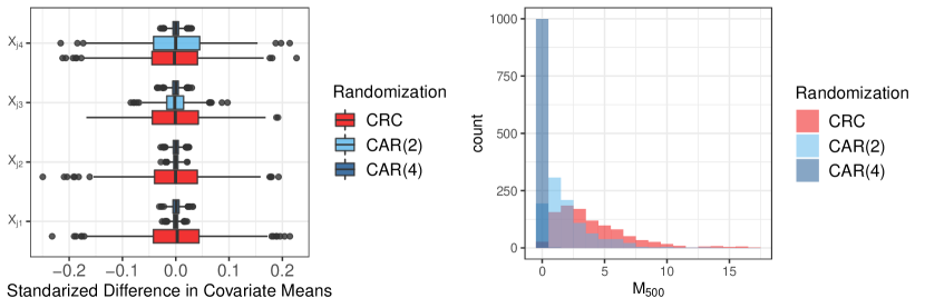
Figure 1: The standardized difference in means for $\bm{X}_{j}$ and the Mahalanobis distance when $\alpha=0.5$, $r=0.1$, given the hypothetical network, based on 1000 runs. The Mahalanobis distance is calculated for all four covariates of the clusters.

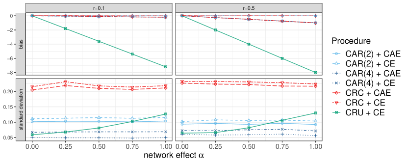
Figure 2: The bias and standard deviation of the estimated ATE versus network effect $\alpha$ given the hypothetical network, based on 1000 runs.

Table 1: The bias and standard deviation of the estimated of ATE under different A/B testing procedures given the hypothetical network, based on 1000 runs.

$r$	Randomization	Estimator		$\alpha=0$			$\alpha=1$
	procedure			Bias	s.d.		Bias	s.d.
$0.1$	CAR ($2$)	CAE		0.0057	0.10		-0.0003	0.10
		CE		0.0047	0.11		-0.2005	0.12
	CAR ($4$)	CAE		-0.0022	0.05		0.0025	0.05
		CE		-0.0012	0.07		-0.1976	0.07
	CRC	CAE		0.0002	0.21		0.0027	0.21
		CE		0.0012	0.22		-0.1959	0.22
	CRU	CE		0.0015	0.06		-7.2003	0.12
$0.5$	CAR ($2$)	CAE		-0.0022	0.09		-0.0047	0.09
		CE		-0.0046	0.10		-1.0054	0.10
	CAR ($4$)	CAE		0.0027	0.06		0.0002	0.06
		CE		-0.0003	0.07		-1.0019	0.07
	CRC	CAE		0.0019	0.22		-0.0011	0.22
		CE		-0.0002	0.23		-1.0033	0.23
	CRU	CE		-0.0003	0.06		-7.9999	0.12

Results: Figure 1 shows that the CAR produce more balanced clusters than CRC. The Mahalanobis distance calculated with all four covariates of the clusters is more concentrated at zero, when more covariates are used in CAR. In addition, it can be seen from the boxplot that use of the covariates in CAR will result in a small variance of a standardized difference of the covariates mean. These results show the superior balance properties of the CAR procedure.

Table 2: The $PRIV(\hat{\tau}_{CAE}|CAR)$ given the hypothetical network, based on 1000 runs.

$r$	CAR		$\alpha=0$	$\alpha=1$
0.1	(2)		75.67	74.93
	(4)		93.86	94.46
0.5	(2)		82.67	82.95
	(4)		92.86	93.27

It can be seen from Table 1 and Figure 2 that all of the A/B testing procedures are consistent, i.e., bias is about zero, when there is no network effect. In this case, the classical A/B testing procedure works well. As the network effect increases, the bias using the classical A/B testing procedure increases dramatically, i.e., the bias under CRU following with CE is above 7, when $\alpha=1$.

The network A/B testing procedures using CE, i.e., CAR following with CE and CRC following with CE, are less biased than the classical method. Comparing the bias obtained from these procedures for $r=0.1$ and $r=0.5$, it can be seen that these methods work well when the clusters are less connected, i.e., $r=0.1$. When the connections between the clusters increase, the biases of these procedures are not negligible. For example, when $r=0.5$, the bias of CAR following with CE is -0.1976. This is because the effects obtained from linked clusters, which can bias the estimation, are not removed if CE is used for estimation. On the other hand, the network A/B testing procedure using CAE, i.e., CAR following with CAE and CRC using CAE, is consistent for all of the parameter settings. These results justify Theorem 2.2 and suggest that if the network effect is not eliminated appropriately, the bias will still increase as the network effect increases.

From Table 1 and Figure 2, it can be seen that using CAR procedure can significantly reduce the standard deviation of the estimators of the ATE. Comparing the performance of CAR (2) and CAR (4), the standard deviation decreases as more covariates of the clusters are used in CAR. This suggests that the efficiency of the estimation will increase if more important features of the clusters can be used in CAR. Furthermore, Table 2 shows that the improvement of using CAR is above $70\%$. In particular, using all four covariates in CAR can improve at least $93\%$ of the variance for the estimation of ATE. These results suggest that using our cluster-adaptive network A/B testing procedure is able to not only reduce the bias but also improve the estimation efficiency.

4 The MIT Phone Call Network

The MIT Phone Call Network listed in the Network Data Repository Rossi and Ahmed, (2015) is used to illustrate how our cluster-adaptive network A/B testing procedure works for real world social networks. The network consists of phone calls/voicemails between a group of users at MIT, where vertices and edges represent users and calls/voicemails, respectively Eagle and Pentland, (2006). In addition, the network is labeled with 82 clusters via label propagation algorithm Raghavan et al., (2007) (see Figure 3). The response of users is generated with the same parameter settings as in Section 3. The A/B testing procedures used in Section 3 are also compared for the MIT phone call network.

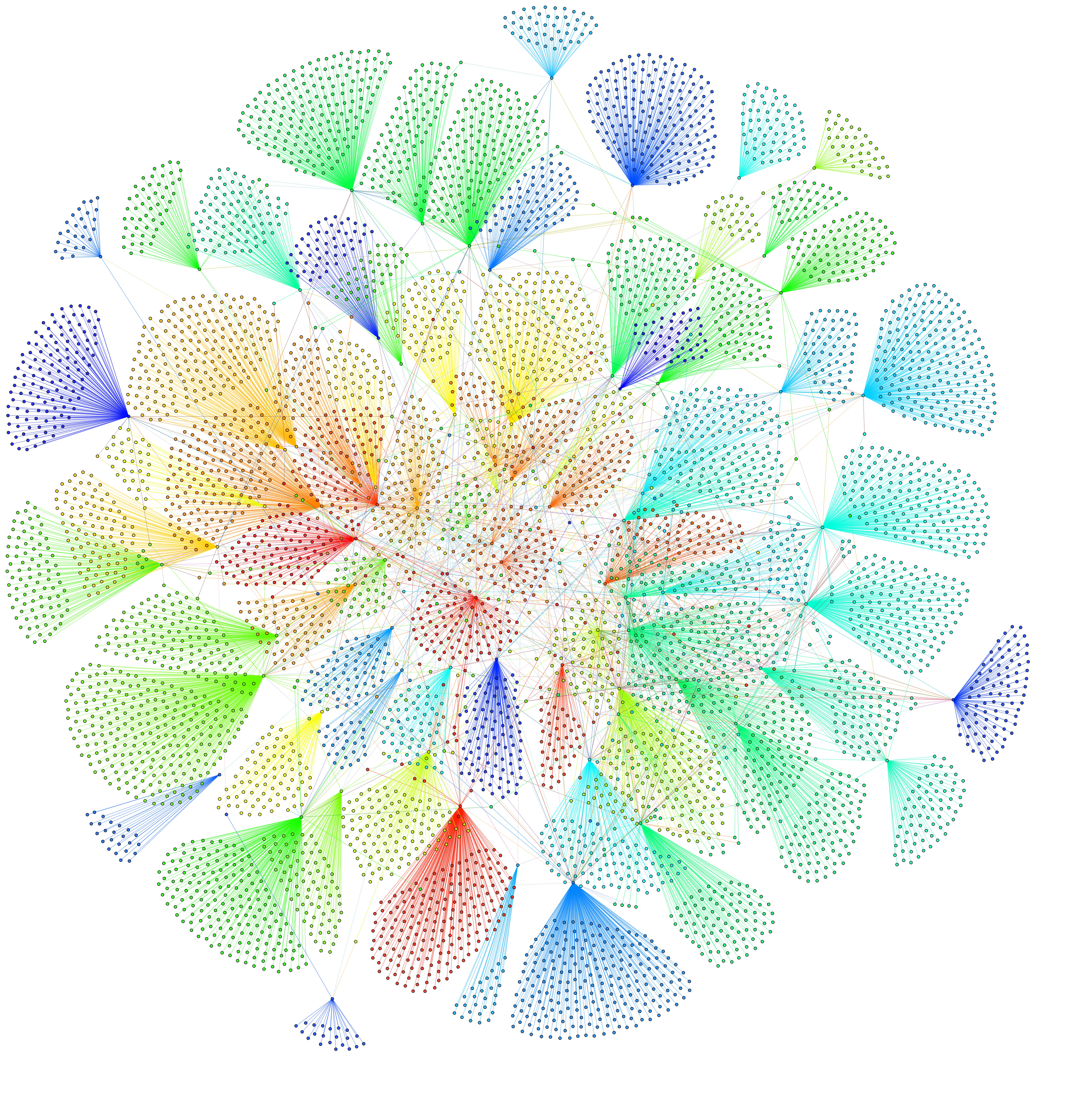
Figure 3: MIT phone call network: There are 6819 vertices and 7768 edges, which are colored by labels of the clusters.

For the numerical comparison, we consider that all four covariates of the cluster are used for CAR. The bias and standard deviation of the estimated ATE under the setting of $\alpha\in\{0,1\}$ are presented in Table 3. The simulation results exploring other parameter settings are presented in Figures 4.

Results: Similar to the results presented in the previous section, the classical A/B testing procedure works well when there is no network effect. However, bias caused by using this method increases dramatically as the network effect increases. Comparing with the values under CRU, CE under CAR and CRC are moderately biased. CAE under CAR and CRC are consistent for the estimation of the ATE, so that the biases are about zero. It can be seen from Figure 4 and Table 3 that our cluster-adaptive network A/B testing procedure has much smaller standard deviation compared to CRC following with CAE. According to our simulations, $PRIV(\hat{\tau}_{CAE}|CAR)$ under $\alpha=0$ and $\alpha=1$ are $84.52\%$ and $84.55\%$, respectively. These results suggest that using our cluster-adaptive network A/B testing procedure is able to not only reduce the bias caused by the MIT phone call network but also improve efficiency for estimation of the ATE.

Figure 4: The bias and standard deviation of the estimated ATE versus network effect $\alpha$ given the MIT phone call network, based on 1000 runs.

Table 3: The bias and standard deviation of the estimated ATE given the MIT phone call network, based on 1000 runs.

Randomization	Estimator		$\alpha=0$			$\alpha=1$
Procedure			Bias	s.d.		Bias	s.d.
CAR	CAE		0.005	0.21		0.011	0.21
	CE		0.002	0.43		-0.292	0.44
CRC	CAE		-0.032	0.54		-0.024	0.53
	CE		-0.037	0.78		-0.313	0.75
CRU	CE		-0.003	0.08		-2.281	0.09

5 Conclusion

In this paper, we propose a cluster-adaptive network A/B testing procedure which consists of a cluster-adaptive randomization and a cluster-adjusted estimator. Utilizing the cluster features to produce balanced treatment arms of clusters, the proposed cluster-adaptive randomization is able to improve the estimation efficiency by reducing the variance of the ATE estimator. The cluster-adjusted estimator, which eliminates the network effect gotten from linked clusters and adjusts the inflated cluster effect, achieves a consistent estimation for the ATE, when the employed randomization satisfies the balance condition (8). Numerical studies suggest that our cluster-adaptive network A/B testing procedure outperforms other methods, as it can produce consistent estimation and reduce the variance of the estimator. These results offer a new angle to study the network A/B testing problem. The randomization steps should take the balance of the cluster features into account, so that the treatment arms are more comparable. Moreover, the balanced treatment arms may improve the estimation of the ATE. These ideas are valuable in both theoretical and applied aspects, and can help in the design and analysis of novel network A/B testing procedures.

6 Broader Impact

Any social network based on data driven methods are in potential risk of privacy leakage and ethical problems. Though the usage of network information can improve the decision-making process, researchers have to be aware of some other consequences caused by their algorithm. In this paper, features of clusters in a social network are utilized to improve the results of network A/B testing. In practice, ethical and privacy concerns should be taken into account for the choice of the features put into the algorithm. It can be seen from the simulation results that even if not all of the features are put into the algorithm, the bias and efficiency can still be improved a lot. Therefore, if the sensitive features, which may introduce potential risks, are not used, the cluster adaptive network A/B testing procedure still works well. Therefore, some of the potential risks can be avoided by the appropriate choice of the features used in the algorithm. The proposed procedure can be implemented in many fields comprising drug development, economics, E-commerce, finance, network data analysis and online testing.

Appendix A Proof of the Main Results

A.1 Proof of Theorem 2.1.

Theorem 2.1 characterizes the balance property of CAR. It shows that as the number of clusters increases the Mahalanobis distance converges to zero in probability, so that the standardized difference of the mean for the clusters’ covariates is minimized as well. As a result, the treatment arms are more feasibly compared.

Proof of Theorem 2.1.

Similar to the approach in [18], this proof consists of the following two main steps.

1. First, let $\Sigma=\text{Cov}[\bm{X}_{j}]>0$, and $\xi_{j}=\Sigma^{-1/2}\left(\bm{X}_{j}-\mathbb{E}[\bm{X}_{j}]\right)$, where $\Sigma^{-1/2}$ is the Cholesky square root of $\Sigma^{-1}$. Therefore, $\mathbb{E}[\bm{\xi}_{j}]=0$ and $\operatorname{cov}[\bm{\xi}_{j}]=\mathbf{I}$. Consider

   $$\tilde{M}_{m} =\frac{m}{4}\left(\bar{\bm{X}}_{A}-\bar{\bm{X}}_{B}\right)^{\text{t}}\Sigma^{-1}\left(\bar{\bm{X}}_{A}-\bar{\bm{X}}_{B}\right)$$

   $$=\frac{m}{4}\left(\bar{\bm{\xi}}_{A}-\bar{\bm{\xi}}_{B}\right)^{\text{t}}\left(\bar{\bm{\xi}}_{A}-\bar{\bm{\xi}}_{B}\right),$$ (12)

   where $\bar{\bm{\xi}}_{A}$ and $\bar{\bm{\xi}}_{B}$ are the sample averages of $\bm{\xi}_{j}$ for treatments $A$ and $B$, respectively. Using the drift condition [13], we prove that $\tilde{M}_{m}=O_{P}(m^{-1})$ in Lemma A.1.

2. As $m\to\infty$, $\operatorname{cov}(\bm{X})\stackrel{{\scriptstyle\mathscr{P}}}{{\longrightarrow}}\Sigma$, then it follows from Lemma A.1, the continuous mapping theorem, and the Slutsky’s theorem, that (6) in Theorem 2.1 follows.

∎

The key ingredient for the proof of Theorem 2.1 is presented in the following lemma.

Lemma A.1.

Under the condition of Theorem 2.1, $\{m\tilde{M}_{m}\}_{m=1}^{\infty}$ is a sequence of Harris recurrent Markov chains, and $\tilde{M}_{m}=O_{p}(m^{-1})$.

Proof of Lemma A.1..

By (12), it can be seen that

$$\tilde{M}_{m}=\frac{1}{m}\bm{\eta}_{m}^{\text{t}}\bm{\eta}_{m},$$

where $\bm{\eta}_{m}=\frac{m}{2}\left(\bar{\bm{\xi}}_{A}-\bar{\bm{\xi}}_{B}\right)=\sum_{T_{j}=1}\bm{\xi}_{j}-\sum_{T_{j}=0}\bm{\xi}_{j}$. Then if we can show $\bm{\eta}_{m}$ follows a stationary distribution, then it follows that $\bm{\eta}_{m}^{\text{t}}\bm{\eta}_{m}=O_{p}(1)$. Therefore, Lemma A.1 follows from Slutsky’s theorem.

In order to verify that $\bm{\eta}_{m}$ follows a stationary distribution, consider verifying the drift condition, i.e., (iii) of Theorem 11.0.1. in [13]. Define $\bm{V}(\bm{\eta}_{m})=\bm{\eta}_{m}^{\text{t}}\bm{\eta}_{m}$ as the test function and

$$\bm{\Delta}_{m+2} =\bm{\eta}_{m+2}-\bm{\eta}_{m}$$

$$=(-1)^{T_{m+2}}(\xi_{m+1}-\xi_{m+2}),$$

where $\{\bm{\eta}_{2k}\}_{k=1}^{\infty}$ is a Markov process. To calculate the test function, let $\mathbb{E}[\cdot|\bm{\eta}_{m}]=\mathbb{E}_{m}[\cdot]$. It follows that

$$\mathbb{E}_{m}[\bm{V}(\bm{\eta}_{m+2})]-\bm{V}(\bm{\eta}_{m}) =2\bm{\bm{\eta}}_{m}^{\text{t}}\mathbb{E}_{m}\left[\bm{\Delta}_{m+2}\right]+\mathbb{E}_{m}\left[\bm{\Delta}_{m+2}^{\text{t}}\bm{\Delta}_{m+2}\right],$$ (13)

where $\mathbb{E}_{m}[\bm{\Delta}_{m+2}^{\text{t}}\bm{\Delta}_{m+2}]=\mathbb{E}_{n}\left[(-1)^{2T_{m+2}}(\bm{\xi}_{n+1}-\bm{\xi}_{n+2})^{\text{t}}(\bm{\xi}_{n+1}-\bm{\xi}_{n+2})\right]\geq 0$. For the first term in (13), it follows that

$$\bm{\eta}_{m}^{\text{t}}\mathbb{E}_{m}[\bm{\Delta}_{m+2}] =\mathbb{E}_{m}\left[\mathbb{E}\left[(-1)^{T_{m+2}}\bm{\eta}_{m}^{\text{t}}(\bm{\xi}_{m+1}-\bm{\xi}_{m+2})|\bm{\eta}_{m},\bm{\xi}_{m+1},\bm{\xi}_{m+2}\right]\right]$$

$$=\mathbb{E}_{m}\left[(1-2q)\left|\bm{\eta}_{m}^{\text{t}}(\bm{\xi}_{m+1}-\bm{\xi}_{m+2})\right|\right]$$

$$=(1-2q)\left|\bm{\eta}_{m}\right|\cdot\mathbb{E}_{m}\left[\left|\bm{\xi}_{m+1}-\bm{\xi}_{m+2}\right|\right]\cdot\mathbb{E}\left[|cos\theta|\right],$$

where $\theta$ is the angle between $\bm{\eta}_{m}$ and $\bm{\xi}_{m+1}-\bm{m+2}$. Here, $\mathbb{E}_{m}\left[\left|\bm{\xi}_{m+1}-\bm{\xi}_{m+2}\right|\right]$ and $\mathbb{E}\left[|cos\theta|\right]$ are two positive constants. It follows from $q>1/2$ that there exist constants $b>0,c>0$ such that

$$\begin{array}[]{lll}\mathbb{E}_{m}\left[\bm{V}(\bm{\eta}_{m+2})\right]-\bm{V}(\bm{\eta}_{m})<-c&\textit{for}\ \ |\bm{\eta}_{m}|>b&and\\ \mathbb{E}_{m}\left[\bm{V}(\bm{\eta}_{m+2})\right]-\bm{V}(\bm{\eta}_{m})<\mathbb{E}_{m}\left[\bm{\Delta}_{m+2}^{\text{t}}\bm{\Delta}_{m+2}\right]&\textit{ for}\ \ |\bm{\eta}_{m}|\leq b.\end{array}$$

Therefore, the drift condition is checked and the proof of the lemma is completed.

∎

A.2 Proof of Theorem 2.2.

The representation of CAE, i.e., (7), not only shows that CAE can eliminate the network effect, but also provides a way to study the asymptotic behavior of CAE. Theorem 2.2 only studies the consistency with the balance condition (8). If more assumptions of network and the randomization procedure are provided, the asymptotic normality could be derived via (7). The proof of Theorem 2.2 is shown as follows.

Proof of Theorem 2.2..

Under the assumption of Theorem 2.2, we rewrite the response model as follows. For $i\in\mathcal{C}_{j},$

$$Y_{i} =\mu_{0}(1-Z_{i})+\mu_{1}Z_{i}+\bm{\beta}\bm{X}_{j}+\sum_{k\in\mathcal{C}_{j}}\gamma_{ki}+\sum_{k\notin\mathcal{C}_{j}}\gamma_{ki}+\epsilon_{i},$$

where $\gamma_{ki}=\alpha_{0}A_{ik}Z_{k}(Z_{i}-1)+\alpha_{1}A_{ki}(Z_{k}-1)Z_{i}$ and $A_{ik}$ is the component of row $i$ column $k$ for the adjacent matrix $A$. If the employed randomization is performed on clusters, then $\sum_{k\in\mathcal{C}_{j}}\gamma_{ki}=0$ as $Z_{k}=Z_{i}$, for $i,k\in\mathcal{C}_{j}$. If the users used for estimation are all from the uncontaminated set, i.e., $\mathcal{U}=\{i:\bm{A}_{i*}(\bm{1}-\bm{Z})=0\text{ and }Z_{i}=1\}\cup\{i:\bm{A}_{i*}\bm{Z}=0\text{ and }Z_{i}=0\},$ then $\sum_{k\notin\mathcal{C}_{j}}\gamma_{ki}=0$ for $i\in\mathcal{U}$. Therefore, it follows that

$$Y_{i}=\mu_{0}(1-Z_{i})+\mu_{1}Z_{i}+\bm{\beta}^{\text{t}}\bm{X}_{j}+\epsilon_{i}.$$ (14)

It can be seen from (14) that the network effect is eliminated and (7) in Theorem 2.2 follows.

Now we show that $\hat{\tau}_{CAE}$ is consistent. Note that the users’ cluster features will have the same value if the users are in the same cluster, so

$$\bar{W}_{j}(\mathcal{U}) =\frac{1}{n_{j}(\mathcal{U})}\sum_{i\in\mathcal{C}_{j}\cap\mathcal{U}}(\bm{X}_{j}^{\text{t}}\bm{\beta}+\epsilon_{i})$$

$$=\bm{X}_{j}^{\text{t}}\bm{\beta}_{j}+\frac{1}{n_{j}(\mathcal{U})}\sum_{i\in\mathcal{C}_{j}\cap\mathcal{U}}\epsilon_{i}.$$

According to assumption (8) in Theorem 2.2, it is easy to see that

$$\begin{array}[]{cccc}\frac{m_{A}}{m}\stackrel{{\scriptstyle\mathscr{P}}}{{\longrightarrow}}1/2&\frac{m_{b}}{m}\stackrel{{\scriptstyle\mathscr{P}}}{{\longrightarrow}}1/2&and&\frac{1}{m}\sum_{j=1}^{m}(2T_{j}-1)\bm{X}_{j}^{\text{t}}\bm{\beta}\stackrel{{\scriptstyle\mathscr{P}}}{{\longrightarrow}}0.\end{array}$$

Then the consistency of $\hat{\tau}_{CAE}$ follows from Slutsky’s theorem and

$$\frac{1}{m}\sum_{j=1}^{m}\frac{2T_{j}-1}{n_{j}(\mathcal{U})}\sum_{i\in\mathcal{C}_{j}\cap\mathcal{U}}\epsilon_{i}\stackrel{{\scriptstyle\mathscr{P}}}{{\longrightarrow}}0,$$ (15)

which can be shown by Chebyshev’s inequality, provided that $\epsilon_{i}$ are i.i.d. with mean zero and variance $\sigma_{\epsilon}^{2}<\infty$.

∎

A.3 Proof of Corollary 2.1.

Proof of Corollary 2.1..

1. Under CRC, $T_{j}\stackrel{{\scriptstyle i.i.d.}}{{\sim}}Bernoulli(1/2)$ and $\bm{X}_{j}\perp T_{j}$, then

   $$\begin{array}[]{ccc}\mathbb{E}[2T_{j}-1]=0&and&\mathbb{E}[(2T_{j}-1)\bm{X}_{j}]=0.\end{array}$$

   Therefore, (8) in Theorem 2.2 follows from WLLN.

2. Under CAR, assume $m$ is even, then $m_{A}=m_{B}=m/2$ a.s. and $2\sum_{j=1}^{m}T_{j}-1=m_{A}-m_{B}=0$. According to the proof of Lemma 3.1., $\bm{\eta}_{m}$ follows a stationary distribution. It follows that

   $$\bar{\bm{X}}_{A}-\bar{\bm{X}}_{B} =\frac{2}{m}(\bar{\bm{\xi}}_{A}-\bar{\bm{\xi}}_{B})=\frac{2}{m}\cdot\bm{\eta}_{m}$$

   $$=O_{p}\left(\frac{1}{m}\right),$$

   Therefore, the balance condition in Theorem 2.2. follows.

The balance condition is checked for CRC and CAR, hence the proof of Corollary 2.1 is completed. ∎

A.4 Proof of Theorem 2.3.

Theorem 2.4 shows the benefit of using CAR to produce balanced treatment arms in the estimation of the ATE. As the lower bound in (10) is positive, using CAR following with CAE will be more efficient than using CRC following with CAE. This result can further imply that the valid statistical inference for the ATE, i.e., the test that obtains the correct type I error, using our cluster-adaptive network A/B testing, can achieve higher power and tighter confidence intervals. These results are left for future studies. The proof of Theorem 2.4 is as follows.

Proof of Theorem 2.4..

Suppose the pseudo response variables $Y_{j}^{P}$ on the cluster level are generated by the same additive linear model

$$Y^{P}_{j}=\mu_{0}(1-T_{j})+\mu_{1}T_{j}+\bm{\beta}^{\text{t}}\bm{X}_{j}+\epsilon_{j},$$

where $\epsilon_{j}$ has the same distribution as $\epsilon_{i}$ in the response model for each user. Then the ATE based on pseudo response variables is

$$\hat{\tau}^{C} =\frac{1}{m_{A}}\sum_{j=1}^{m}T_{j}Y_{j}^{P}-\frac{1}{m_{B}}\sum_{j=1}^{m}(1-T_{j})Y_{j}^{P}$$

$$\simeq\tau+\bm{\beta}^{\text{t}}(\overline{\bm{X}}_{A}-\overline{\bm{X}}_{B})+\frac{2}{m}\sum_{j=1}^{m}(2T_{j}-1)\epsilon_{j},$$

where $\bar{\bm{X}}_{A}$, $\bar{\bm{X}}_{B}$ are the sample means of cluster covariates in treatments A and B, respectively. Here $\hat{\tau}^{C}$ is a pseudo treatment effect estimator, which assumes that each cluster has only one response.

The adjusted cluster-level estimator $\hat{\tau}_{CAE}$ only uses the sample average of the $n_{j}(\mathcal{U})$ users in cluster $\mathcal{C}_{j}$, i.e.,

$$\overline{Y}_{j}(\mathcal{U})=\mu_{0}(1-T_{j})+\mu_{1}T_{j}+\bm{\beta}^{\text{t}}\bm{X}_{j}+\frac{1}{n_{j}(\mathcal{U})}\sum_{i\in\mathcal{C}_{j}\cap\mathcal{U}}\epsilon_{i}.$$

Then CAE can be written as

$$\hat{\tau}_{CAE} =\frac{1}{m_{A}}\sum_{j=1}^{m}T_{j}\bar{Y}_{j}(\mathcal{U})-\frac{1}{m_{B}}\sum_{j=1}^{m}(1-T_{j})\bar{Y}_{j}(\mathcal{U})$$

$$\simeq\tau+\bm{\beta}^{\text{t}}(\overline{\bm{X}}_{A}-\overline{\bm{X}}_{B})+\frac{2}{m}\sum_{j=1}^{m}\frac{2T_{j}-1}{n_{j}(\mathcal{U})}\sum_{i\in\mathcal{C}_{j}\cap\mathcal{U}}\epsilon_{i},$$

$$where\leavevmode\nobreak\ \operatorname{var}\left[\frac{2}{m}\sum_{j=1}^{m}\frac{2T_{j}-1}{n_{j}(\mathcal{U})}\sum_{i\in\mathcal{C}_{j}\cap\mathcal{U}}\epsilon_{i}\right]=\frac{4}{m^{2}}\sum_{j=1}^{m}\frac{\sigma_{\epsilon}^{2}}{n_{j}(\mathcal{U})}.$$

Denote $*$ as one of CAR or CRC. Then, the variances for two types of estimators under a given randomization * are

$$\operatorname{var}[\hat{\tau}^{C}|*] \simeq\bm{\beta}^{\text{t}}\operatorname{cov}[\overline{\bm{X}}_{A}-\overline{\bm{X}}_{B}|*]\bm{\beta}+\operatorname{var}\left[\frac{2}{m}\sum_{j=1}^{m}(2T_{j}-1)\epsilon_{j}\right]$$

$$=\bm{\beta}^{\text{t}}\operatorname{cov}[\overline{\bm{X}}_{A}-\overline{\bm{X}}_{B}|*]\bm{\beta}+\frac{4}{m}\sigma_{\epsilon}^{2},\ \ \ \ and$$

$$\operatorname{var}[\hat{\tau}_{CAE}|*] \simeq\bm{\beta}^{\text{t}}\operatorname{cov}[\overline{\bm{X}}_{A}-\overline{\bm{X}}_{B}|*]\bm{\beta}+\frac{4}{m^{2}}\sum_{j=1}^{m}\frac{\sigma_{\epsilon}^{2}}{n_{j}(\mathcal{U})}$$

$$\leq\bm{\beta}^{\text{t}}\operatorname{cov}[\overline{\bm{X}}_{A}-\overline{\bm{X}}_{B}|*]\bm{\beta}+\frac{4}{m}\frac{1}{\min_{j}n_{j}(\mathcal{U})}\sigma_{\epsilon}^{2}$$

$$\leq\operatorname{var}[\hat{\tau}^{C}|*].$$

Then, under any randomization procedure $*$ we have

$$\operatorname{var}[\hat{\tau}_{CAE}|*]-\operatorname{var}[\hat{\tau}^{C}|*] =\frac{4}{m}\left[\frac{1}{m}\cdot\sum_{j=1}^{m}\frac{1}{n_{j}(\mathcal{U})}-1\right]\sigma_{\epsilon}^{2}:=C_{1}\sigma_{\epsilon}^{2},$$

where $C_{1}$ is some constant depending on $\mathcal{G}$. As $n_{j}(\mathcal{U})\geq 1$, it can be seen that $C_{1}\leq 0$ ($C_{1}=0$ when $n_{j}(\mathcal{U})=1$ for $j=1,\cdots,m$). By Theorem 3.2. in [18], it follows that

$$PRIV(\tau^{C}|CAR)=\frac{\operatorname{var}[\hat{\tau}^{C}|CR]-\operatorname{var}[\hat{\tau}^{C}|CAR]}{\operatorname{var}[\hat{\tau}^{C}|CR]}=(1-\frac{\mathbb{E}[M_{m}|CAR]}{p})R_{C}^{2},$$

and hence

$$PRIV(\hat{\tau}_{CAE}|CAR) =\frac{\operatorname{var}[\hat{\tau}_{CAE}|CRC]-\operatorname{var}[\hat{\tau}_{CAE}|CAR]}{\operatorname{var}[\hat{\tau}_{CAE}|CRC]}$$

$$=\frac{(\operatorname{var}[\hat{\tau}^{C}|CRC]+C_{1}\sigma_{e}^{2})-(\operatorname{var}[\hat{\tau}^{C}|CAR]+C_{1}\sigma_{e}^{2})}{\operatorname{var}[\hat{\tau}_{CAE}|CRC]}$$

$$=(1-\frac{\mathbb{E}[M_{m}|CAR]}{p})\cdot R_{C}^{2}\cdot\frac{\operatorname{var}[\hat{\tau}^{C}|CR]}{\operatorname{var}[\hat{\tau}_{CAE}|CRC]}$$

$$\geq(1-\frac{\mathbb{E}[M_{m}|CAR]}{p})R_{C}^{2}.$$

This completes the proof of the theorem. ∎

Appendix B The Hypothetical Network

In this section, we study the properties of our cluster-adaptive network A/B testing procedure under different structures of the hypothetical network. Specially, we are interested in the performance of our procedure when the number of edges connecting different clusters increases.

We use the same hypothetical network as in Section 3. First, 500 independent clusters are generated by the Watts-Strogatz small-world model. For $j=1,\cdots,500$, we generate the cluster size $n_{j}$ from a symmetric discrete distribution, $\mathbb{P}(n_{j}=\lambda)=\left[\left(|\lambda-20|+0.5\right)\sum_{\lambda=10}^{30}(1/\left(|\lambda-20|+0.5\right)\right]^{-1}$, where $\lambda=10,...,30$. Therefore, $N=\sum_{j=1}^{500}n_{j}$ users are involved in this network. In addition, $r\times N$ edges are randomly added, so that several clusters are connected, where $r$ is chosen as the re-connection probability.

Consider the response $Y_{i}$ follows the assumed response model (16) with $p=4$ and $\epsilon_{i}\sim N(0,2^{2})$. The covariates of the clusters, i.e., $\bm{X}_{j}=(X_{j1},\cdots,X_{j4})^{\text{t}}$, involved in the response model are the number of vertices in $\mathcal{C}_{j}$ ($X_{j1}$), the number of edges in $\mathcal{C}_{j}$ ($X_{j2}$), the number of edges in $\mathcal{C}_{j}$ with other clusters ($X_{j3}$), and the density of $\mathcal{C}_{j}$ ($X_{j4}$). In addition, consider $\alpha_{1}=-\alpha_{0}=\alpha=0.5$ for the network spill-over effect, $\beta_{1}=\cdots=\beta_{4}=1$ for the effect of clusters’ covariates, and $\tau=\mu_{1}-\mu_{0}=1$ for the treatment effect.

$$Y_{i}=\mu_{0}(1-Z_{i})+\mu_{1}Z_{i}+\alpha_{0}\bm{A}_{i*}\bm{Z}(Z_{i}-1)+\alpha_{1}\bm{A}_{i*}(\bm{Z}-\bm{1})Z_{i}+\bm{\beta}^{\text{t}}\bm{X}_{j}+\epsilon_{i},$$ (16)

To compare with other network A/B testing procedures, we consider the classic A/B testing procedure, i.e., complete randomization with users (CRU), following with the classical estimator (CE), and graph clustering procedure using the complete randomization on clusters (CRC), following with CE and CAE. For our CAR method, we consider two cases, 1) CAR (2), CAR using the first two covariates $X_{j1}$ and $X_{j2}$, and 2) CAR (4), CAR using all of the four covariates $X_{j1},\cdots,X_{j4}$. The Mahalanobis distance and the standardized difference in covariate means for $\bm{X}_{j}$ are presented in Figure 5 and Figure 6 to compare the balance properties of the randomization procedures. We compare the performance of these A/B testing procedures for the hypothetical network with $r=0.1,0.2,\cdots,2.$

Table 4 summarizes the bias and standard deviation (s.d.) of the estimated ATE for $r=0.5,1,1.5$ and 2. Furthermore, we study the $PRIV(\hat{\tau}_{CAE}|CAR)$ and its’ corresponding lower bound (L-B) in Table 5 for $r=0.5,1,1.5,$ and $2$. Figure 7 summarizes the bias and the standard deviation of the estimated ATE, and the $PRIV(\hat{\tau}_{CAE}|CAR)$ and its corresponding lower bound for all different settings of $r$. Note that the lower bound of $PRIV(\hat{\tau}_{CAE}|CAR)$ for CAR (4), i.e., L-B (4), is calculated from (10) in Theorem 2.3 with the Mahalanobis distance using all four covariates and $R^{2}_{C}$ calculated according to the pseudo response model (11) with all four cluster covariates, whereas the lower bound of $PRIV(\hat{\tau}_{CAE}|CAR)$ for CAR (2), i.e., L-B (2), is calculated with the Mahalanobis distance using the first two covariates used in randomization and $R^{2}_{C}$ calculated according to the pseudo response model (11) with only the first two covariates.

Results: Figure 5 and Figure 6 show that CAR produces better balance for the clusters’ covariates than CRC under different network settings. In particular, CAR (4) outperforms other procedures for all values of $r$. It can be seen from Figure 6 that the standard deviation for each component of $\bm{X}_{j}$ are the smallest under CAR (4). The two covariates used in CAR (2) have small standard deviations as well, but the two covariates not used in CAR (2) have slightly larger standard deviations. In addition, Figure 5 shows that the Mahalanobis distances calculated with all four covariates are centered at zero for CAR(4) for all settings of $r$. The values under CAR (2) are less centered than the corresponding values under CAR(4), but are more centered than the values under CRC. These results show that the standardized difference in means for the clusters’ covariates and the Mahalanobis distance are much more centered around zero under CAR. As a result, the differences of distributions of the clusters’ covariates between treatment A and treatment B are much smaller under CAR, and the two treatment groups are more feasibly compared.

Figure 5: The Mahalanobis distance given the hypothetical network, based on 1000 runs. The Mahalanobis distance is calculated for all four covariates of the clusters.

Table 4 and Figure 7 show that the network A/B testing procedures using CAE, i.e., CAR following with CAE and CRC following with CAE, are unbiased for all values of $r$. On the other hand, the bias of CE increases as $r$ increases under CAR, CRC, and CRU. It can be seen that CE is less biased under CRC and CAR than the value under CRU. This is because CRC and CAR are performed on clusters, so that the network spill-over effect obtained from the users within the same cluster is removed. However, the network spill-over effect obtained from the users from the linked clusters still exists. Therefore, the bias under CAR and CRC still increases as $r$ increases.

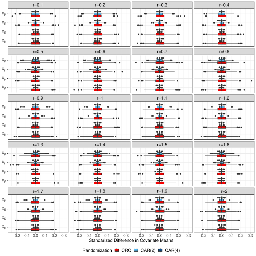
Figure 6: The standardized difference in means for $\bm{X}_{j}$, given the hypothetical network, based on 1000 runs.

To further compare the unbiased network A/B testing procedures, it can be seen from Table 4 and Figure 7 that using CAE under CAR (4) results in the smallest standard deviation among all of the unbiased procedures. The performance of using CAE under CAR (2) is also better than the performance of using CAE under CRC. In addition, as the value of $r$ increases, the standard deviation of the CAE increases. This is because that, as $r$ increases, the number of edges connecting different clusters increases, and thus the number of users in the uncontaminated set decreases. When fewer users can be used for estimation, the efficiency of CAE will decrease. When $r=2$, which means that there are $2\times N$ edges among the clusters, the results still show that using CAR together with CAE is more efficient than CRC, as the PRIVs are about 70% and 64%, respectively.

Table 4: The bias and the standard deviation (s.d.) of the estimated ATE under different A/B testing procedures given the hypothetical network, based on 1000 runs.

Randomization	Estimation		$r=0.5$			$r=1$			$r=1.5$			$r=2$
			bias	s.d.		bias	s.d.		bias	s.d.		bias	s.d.
CAR(2)	CAE		0.00	0.09		-0.00	0.10		-0.01	0.12		-0.01	0.16
	CE		-0.50	0.11		-1.00	0.10		-1.50	0.10		-2.00	0.09
CAR(4)	CAE		-0.00	0.06		0.00	0.08		0.00	0.11		0.00	0.14
	CE		-0.50	0.07		-1.00	0.08		-1.50	0.08		-2.00	0.08
CRC	CAE		0.00	0.22		0.01	0.24		0.01	0.24		-0.00	0.26
	CE		-0.50	0.23		-1.00	0.25		-1.50	0.24		-2.00	0.24
CRU	CE		-4.00	0.08		-4.50	0.08		-5.00	0.09		-5.50	0.09

Figure 7: The bias and standard deviation of the estimated ATE, and the $PRIV(\hat{\tau}_{CAE}|CAR)$ and the corresponding lower bound (L-B) versus the reconnecting probability $r$ given the hypothetical network, based on 1,000 runs.

Table 5: The $PRIV(\hat{\tau}_{CAE}|CAR)$ $(\%)$ and the corresponding lower bound (L-B) for the CAE under CAR , based on 1,000 runs.

CAR		$r=0.5$			$r=1$			$r=1.5$			$r=2$
		PRIV	(L-B)		PRIV	(L-B)		PRIV	(L-B)		PRIV	(L-B)
(2)		82.93	(42.91)		80.75	(43.09)		75.63	(43.16)		64.75	(43.26)
(4)		92.75	(58.76)		89.41	(59.67)		79.85	(60.04)		70.76	(60.53)

Table 5 and Figure 7 show that the $PRIV(\hat{\tau}_{CAE}|CAR)$ for CAR(4) is getting closer to its corresponding lower bound, i.e., L-B CAR (4), as $r$ increases, whereas the lower bound of the $PRIV(\hat{\tau}_{CAE}|CAR)$ for CAR(2) is quite conservative. The reason is that the $R_{c}^{2}$ will be small when it is calculated with only the first two covariates and the true model (11) includes more covariates. The $PRIV(\hat{\tau}_{CAE}|CAR)$ under CAR (2) is above 64%, and its corresponding lower bound is about 43%. The results suggest that when fewer covariates are used in CAR than the number of covariates that we should use, the efficiency of the estimation for the ATE still can be obtained.

Appendix C The MIT Phone Call Network

The MIT phone call Network listed in the Network Data Repository [22] is studied again for two purposes. First, the performance of CAR for the MIT phone call network is presented to demonstrate the advantages of using CAR for real world networks. Second, we compare the bias and standard deviation of the estimated ATE for CAR using the first two clusters’ covariates, i.e., CAR (2), and CAR using all four covariates, i.e., CAR (4), to show that if more balanced treatment arms can be obtained from randomization, then we can obtain a more efficient estimation of the ATE.

The response of the users is generated with the same parameter settings as in Section 3. We consider $\alpha\in\{0,0.25,0.5,0.75,1\}$ for the settings of network spill-over effects. The A/B testing procedures used in Section 3 are also compared for the MIT phone call network.The balance properties of CAR (2), CAR (4), and CRC are also compared. For the simplicity of presentation, we only present the standardized difference in the covariate means for $\bm{X}_{j}$ and the Mahalanobis distance for $\alpha=0$ in Figure 8. As the MIT network is fixed, the balance properties of CAR and CRC for other values of $\alpha$ are similar as presented in Figure 8. Therefore, these results are omitted. Figure 9 summarizes the bias and standard deviation of the estimated ATE for different network A/B testing procedures.

Figure 8: The standardized difference in the covariate means for $\bm{X}_{j}$ and the Mahalanobis distance given the MIT network ($\alpha=0$), based on 1,000 runs.The Mahalanobis distance is calculated with all four covariates of the clusters.

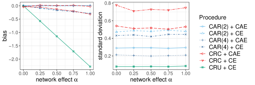
Figure 9: The bias and standard deviation of the estimated ATE versus the network effect $\alpha$ given the MIT network, based on 1,000 runs.

Results: Figure 8 shows that the covariates of the clusters for the MIT Phone call network are more balanced between treatments A and B under CAR. It can be seen from the boxplots that the IQR of the covariates used in CAR are much smaller than the values under CRC. The Mahalanobis distance is much more centered under CAR than the value under CRC. These results illustrate the usage of CAR in improving the balance of clusters’ covariates for the MIT phone call network.

It can be seen from Figure 8 and Figure 9 that using more covariates in CAR can result in more balanced treatment arms and hence more efficient estimation of the ATE. Comparing CAR(2) and CAR(4) in Figure 8, as more covariates are used in CAR, the Mahalanobis distance and the standardized difference in the covariates’ means for $X_{j3}$ and $X_{j4}$ are more centered around zero. Therefore, the increase of the number of covariates used in CAR improves the balance of the clusters’ covariates for treatment A and treatment B. It can be seen from Figure 9 that as treatment A and treatment B are more comparable under CAR (4), the standard deviation of CAE is much smaller than the values under CAR (2).

Appendix D Code

See https://github.com/yzhou12/CAR-network-AB-test for the code and the data used to run the experiments.

References

- Bader et al., [2013] Bader, D. A., Meyerhenke, H., Sanders, P., and Wagner, D. (2013). Graph partitioning and graph clustering, volume 588. American Mathematical Society Providence, RI.
- Bugni et al., [2018] Bugni, F. A., Canay, I. A., and Shaikh, A. M. (2018). Inference under covariate-adaptive randomization. Journal of the American Statistical Association, 113(524):1784–1796.
- Eagle and Pentland, [2006] Eagle, N. and Pentland, A. (2006). Reality mining: sensing complex social systems. Personal and Ubiquitous Computing, 10(4):255–268.
- Eckles et al., [2016] Eckles, D., Karrer, B., and Ugander, J. (2016). Design and analysis of experiments in networks: Reducing bias from interference. Journal of Causal Inference, 5(1).
- Gui et al., [2015] Gui, H., Xu, Y., Bhasin, A., and Han, J. (2015). Network a/b testing: From sampling to estimation. In Proceedings of the 24th International Conference on World Wide Web, WWW ’15, page 399–409, Republic and Canton of Geneva, CHE. International World Wide Web Conferences Steering Committee.
- Hu and Hu, [2012] Hu, Y. and Hu, F. (2012). Asymptotic properties of covariate-adaptive randomization. The Annals of Statistics, 40(3):1794–1815.
- Imbens and Rubin, [2015] Imbens, G. W. and Rubin, D. B. (2015). Causal inference in statistics, social, and biomedical sciences. Cambridge University Press.
- Jiang et al., [2016] Jiang, B., Shi, X., Shang, H., Geng, Z., and Glass, A. (2016). A framework for network ab testing.
- Kohavi et al., [2013] Kohavi, R., Deng, A., Frasca, B., Walker, T., Xu, Y., and Pohlmann, N. (2013). Online controlled experiments at large scale. In Proceedings of the 19th ACM SIGKDD international conference on Knowledge discovery and data mining, pages 1168–1176.
- Kohavi et al., [2014] Kohavi, R., Deng, A., Longbotham, R., and Xu, Y. (2014). Seven rules of thumb for web site experimenters. In Proceedings of the 20th ACM SIGKDD international conference on Knowledge discovery and data mining, pages 1857–1866.
- Ma et al., [2015] Ma, W., Hu, F., and Zhang, L. (2015). Testing hypotheses of covariate-adaptive randomized clinical trials. Journal of the American Statistical Association, 110(510):669–680.
- [12] Ma, W., Qin, Y., Li, Y., and Hu, F. (2020 (to appear)). Statistical inference for covariate-adaptive randomization procedures. Journal of the American Statistical Association.
- Meyn and Tweedie, [2012] Meyn, S. P. and Tweedie, R. L. (2012). Markov chains and stochastic stability. Springer Science & Business Media.
- Middleton and Aronow, [2011] Middleton, J. A. and Aronow, P. M. (2011). Unbiased estimation of the average treatment effect in cluster-randomized experiments. Available at SSRN 1803849.
- Morgan et al., [2012] Morgan, K. L., Rubin, D. B., et al. (2012). Rerandomization to improve covariate balance in experiments. The Annals of Statistics, 40(2):1263–1282.
- Newman, [2006] Newman, M. E. (2006). Modularity and community structure in networks. Proceedings of the national academy of sciences, 103(23):8577–8582.
- Pocock and Simon, [1975] Pocock, S. J. and Simon, R. (1975). Sequential treatment assignment with balancing for prognostic factors in the controlled clinical trial. Biometrics, 31(1):103–115.
- Qin et al., [2016] Qin, Y., Li, Y., Ma, W., and Hu, F. (2016). Pairwise sequential randomization and its properties. arXiv preprint arXiv:1611.02802.
- Raghavan et al., [2007] Raghavan, U. N., Albert, R., and Kumara, S. (2007). Near linear time algorithm to detect community structures in large-scale networks. Phys. Rev. E, 76:036106.
- Rao, [1973] Rao, C. R. (1973). Linear statistical inference and its applications, volume 2. Wiley New York.
- Raudenbush, [1997] Raudenbush, S. W. (1997). Statistical analysis and optimal design for cluster randomized trials. Psychological methods, 2(2):173.
- Rossi and Ahmed, [2015] Rossi, R. A. and Ahmed, N. K. (2015). The network data repository with interactive graph analytics and visualization. In AAAI.
- Saint-Jacques et al., [2019] Saint-Jacques, G., Varshney, M., Simpson, J., and Xu, Y. (2019). Using ego-clusters to measure network effects at linkedin. arXiv preprint arXiv:1903.08755.
- Shao et al., [2010] Shao, J., Yu, X., and Zhong, B. (2010). A theory for testing hypotheses under covariate-adaptive randomization. Biometrika, 97(2):347–360.
- Taves, [1974] Taves, D. R. (1974). Minimization: a new method of assigning patients to treatment and control groups. Clinical Pharmacology & Therapeutics, 15(5):443–453.
- Ugander et al., [2013] Ugander, J., Karrer, B., Backstrom, L., and Kleinberg, J. (2013). Graph cluster randomization: Network exposure to multiple universes. In Proceedings of the 19th ACM SIGKDD International Conference on Knowledge Discovery and Data Mining, KDD ’13, page 329–337, New York, NY, USA. Association for Computing Machinery.