Loss of coherence and coherence protection from a graviton bath
Abstract
We consider a quantum harmonic oscillator coupled with a graviton bath and discuss the loss of coherence in the matter sector due to the matter-graviton vertex interaction. Working in the quantum-field-theory framework, we obtain a master equation by tracing away the gravitational field at the leading order and . We find that the decoherence rate is proportional to the cube of the harmonic trapping frequency and vanishes for a free particle, as expected for a system without a mass quadrupole. Furthermore, our quantum model of graviton emission recovers the known classical formula for gravitational radiation from a classical harmonic oscillator for coherent states with a large occupation number. In addition, we find that the quantum harmonic oscillator eventually settles in a steady state with a remnant coherence of the ground and first excited states. While classical emission of gravitational waves would make the harmonic system loose all of its energy, our quantum field theory model does not allow the number states and to decay via graviton emission. In particular, the superposition of number states is a steady state and never decoheres.
I Introduction
One of the most striking consequences of General relativity is undoubtedly given by gravitational waves misner1973gravitation . Such waves propagate through spacetime itself – are part of it – and interact with all matter making it a universal feature of all experiments. The gravitational waves produced by small objects are however hindered by the smallness of gravitational coupling, whilst the gravitational waves produced by large astronomical bodies become attenuated by the large distances to the Earth. Nevertheless, a hundred years from the prediction of gravitational waves (einstein1916, ; einstein1918gravitationswellen, ) the detection of gravitational waves was announced (abbott2016observation, ).
The feeble strain induced by the passing of gravitational waves has been detected in an optomechanical setup employing suspended mirrors (abbott2016observation, ). Whilst most quantum effects remain suppressed at such scales it has been shown that tiny quantum correlations between the phase of light and the position of the mirrors in the Advanced LIGO detectors imprint a non-negligible signal (yu2020quantum, ). Furthermore, there is substantial progress towards reaching the motional ground state of large mirrors where quantum effects become prominent (abbott2009observation, ; whittle2021approaching, ).
Although a purely classical treatment of the gravitational field still suffices to explain all of the current experimental data it is nonetheless interesting to ask what would be the quantum signature of gravitational waves and several different theoretical approaches have been considered (calzetta1994noise, ; anastopoulos1996quantum, ; anastopoulos2013master, ; riedel2013evidence, ; blencowe2013effective, ; suzuki2015environmental, ; de2015decoherence, ; oniga2016quantum, ; oniga2017quantum, ; quinones2017quantum, ; vedral2020decoherence, ; xu2020toy, ). Recent theoretical works have also investigated the possibility of detecting stochastic graviton noise in the context of gravitational wave observatories (parikh2020noise, ; parikh2020quantum, ; parikh2020signatures, ).
However, discerning between classical models of gravity from the quantum version will necessarily require testing coherent features of gravity which cannot be mimicked by any classical noise source. Such a proposal has been devised by considering the two nearby masses – close enough that they interact gravitationally but far enough apart that all other channels of interaction are strongly suppressed – which can entangle only if the gravitational field exhibits bonafide quantum features (bose2017spin, ) 111The results of bose2017spin were first reported in a conference talk in Bangalore ICTS ., see also marletto2017gravitationally . The underlying mechanism for the quantum entanglement of masses (QGEM) has been analyzed within perturbative quantum gravity (Marshman:2019sne, ; bose2022mechanism, ; Vinckers:2023grv, ; Carney_2019, ; Carney:2021vvt, ) and the framework of the Arnowitt–Desse–Meissner (ADM) approach (danielson2022gravitationally, ), as well as in the path integral approach (christodoulou2023locally, ), and for the massive graviton Elahi:2023ozf . Recent developments include an optomechanical proposal for testing the quantum light-bending interaction Biswas:2022qto , a quantum test of the weak equivalence principle Bose:2022czr , and test whether gravity acts as a quantum entity when measured hanif2023testing .
It is thus interesting to ask whether quantized gravitational waves could also induce coherent effects in quantum systems, which would be difficult to explain using a classical theory of gravity.
In this work, we consider a quantum harmonic oscillator coupled to quantized gravitational waves in the context of perturbative quantum gravity. We first review the results of classical quadrupole radiation emitted by a classical harmonic oscillator (Sec. II). We then obtain the matter-graviton coupling in the laboratory frame of the quantum harmonic oscillator using Fermi normal coordinates (Sec. III). By tracing away the graviton, assumed to be in the vacuum state, we obtain a simple master equation of the Lindblad form (gorini1976completely, ; lindblad1976generators, ) for the quantum harmonic oscillator (Sec. IV). The obtained dynamics have some important features.
-
•
The total energy of the quantum harmonic oscillator and of the emitted gravitons is conserved (Sec. V.1).
-
•
The decay rate for number states with is proportional to the square of its associated energy which can be seen as a consequence of Einstein’s equivalence principle and of the quadrupole nature of gravitational waves (Sec. V.2).
-
•
For small occupation numbers, the classical and quantum predictions begin to differ, with the quantum harmonic oscillator retaining a steady-state coherence. In particular, the quantum harmonic oscillator settles in a remnant coherent combination of the ground and first excited states, which is a distinct quantum signature of graviton emission (Sec. V.3).
-
•
For coherent states with large occupation numbers, we recover exactly the predictions for a classical linear quandrupole. The obtained model can thus be seen as the quantum counterpart of the classical radiation theory (Sec. V.4).
-
•
The decoherence rate scales with the cube of the trapping harmonic frequency, which vanishes for a free particle as expected for a system without a mass quadrupole. In particular, our model predicts that the center-of-mass of an isolated system never decoheres due to quantized gravitational waves (Sec. V.5).
We conclude by discussing briefly the suitability of high frequency mechanical oscillator for distinguishing between classical and quantum gravitational waves (Sec. VI). In Appendix A we provide the exact solution of the dynamics by formally mapping our problem to two-photon processes simaan1978off ; gilles1993two , and in Appendix B we estimate the size of the effect for matter-wave interferometry focusing on the QGEM proposal.
II Classical quadrupole radiation
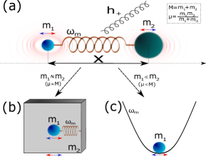
We begin by briefly summarizing the main features of classical gravitational radiation. We recall that gravitational radiation is sourced by a time-dependent mass quadrupole. In this work, we are primarily interested in the motion along one spatial axis where the simplest mass quadrupole is given by a coupled two-particle system (de1986introduction, ) (see Fig. 1). For concreteness we consider two masses, and , coupled by a quadratic potential:
| (1) |
where is the spring constant, and () and () denote the position (momenta) of particle 1 and 2, respectively. It is useful to introduce the center-of-mass coordinates:
| (2) | ||||||
| (3) |
as well as the reduced and total mass
| (4) | ||||
| (5) |
respectively. Using the center-of-mass quantities we find that the potential in Eq. (1) reduces to
| (6) |
where we have defined the harmonic frequency .
We make two well-known observations. On one hand, we note that the center-of-mass remains uncoupled and is thus following a completely free motion (i.e., in the general relativistic language the center-of-mass position follows a geodesic). On the other hand, the relative motion is subject to a quadratic potential which can give rise to a time-dependent linear quadrupole moment (and hence can act as a source of gravitational radiation). In particular, we consider the following relative motion (in the first instance neglecting energy dissipation mechanisms):
| (7) |
where is the amplitude of oscillation of the relative motion. The corresponding quadrupole moment tensor is given by
| (8) |
where is the mass density, , denote the spatial components, and . Inserting in Eq. (8) the mass density
| (9) |
where is given in Eq. (7), we readily find the following non-vanishing elements:
| (10) |
In particular, the linear quadrupole moment gives rise to gravitational radiation of type “+”. The average energy carried away by gravitational waves is given by (de1986introduction, ; maggiore2008gravitational, ):
| (11) |
where we have introduced the moment of inertia . Thus as the two-particle system is oscillating it will slowly lose energy – the amplitude of the relative motion, , will decay, while the center-of-mass motion will remain completely unaffected. Any quantum model of quantized gravitational waves should recover the behaviour of classical quadrupole radiation when the state of the harmonic oscillator can be modeled as approximately classical (i.e., with a coherent state with a large occupation number).
III Linearised quantum gravity
In this section, our working hypothesis is linearised quantum gravity, for a review see (Burgess:2003jk, ). We further assume matter to be non-relativistic, i.e. slowly moving. We find the dominant interaction between matter and graviton in the Fermi normal coordinates (FNC) which does not have any remnant gauge freedom (poisson2011motion, ; misner1973gravitation, ) and is commonly used to describe laboratory experiments (will2006confrontation, ).
III.1 Fermi normal coordinates
For simplicity, we will assume that the relevant motion of the particle is along the -axis and consider the FNC coordinates, , of an ideal observer following a geodesic trajectory (the situation of an observer following a generic time-like curve can be analyzed in a similar fashion). We start from the general relativistic point-particle Lagrangian:
| (12) |
where is the mass of the system222Here denotes a generic mass. In the next Sec. III.2 we will have two such masses, and (see also Fig. 1 for an illustration)., is the speed of light, and is the metric expressed in FNC coordinates. In particular, we write the metric as is the Minkowski metric, and the spacetime curvature perturbation near the geodesic up to order (visser2018post, ). Assuming that matter is moving slowly, the dominant contribution to the dynamics will be given by (rakhmanov2014fermi, ):
| (13) |
where is the “+” component of the gravitational waves usually discussed in the transverse-traceless (TT) coordinates, and is the Riemann tensor component (here denotes the value evaluated on the reference FNC curve).
For completeness, let us sketch how to derive Eq. (14). One can decompose the graviational field into plane waves and Taylor expand then up to order :
| (14) |
where and is the angular frequency of the gravitational field mode. The first term on the RHS of Eq. (14) is a constant and can be omitted, the second term vanishes in FNC coordinates (i.e., linear potentials vanish by choosing an inertial reference frame), while the last term can be rewritten as
| (15) |
where we have used . For a rigorous derivation we refer the reader to (rakhmanov2014fermi, ).
Using Eqs. (12) and (13) we then readily find the interaction Lagrangian between graviton and matter degrees of freedom. Finally, using we find the interaction Hamiltonian
| (16) |
The quadratic coupling in Eq. (16) has been derived by assuming , where is the charachteristic size of the system (implicitly assumed in the expansion in Eq. (14)). The latter condition can be rewritten also as , where we have used (i.e., we assume non-relativistic matter, with the trapped system moving much more slowly than the speed of light).
III.2 Harmonic oscillator coupled to gravitational waves
From Eq. (16) we find that for the two-particle system we have the following interaction Hamiltonian
| (17) |
where () is the position of particle 1 (particle 2). We transform Eq. (17) using the center-of-mass coordinates introduced in Eqs. (2) and (3) to find:
| (18) |
where () is the total (reduced) mass.
From Eq. (18) it would thus appear that the center-of-mass will be more strongly affected by the coupling to the gravitational field than the relative motion (as we always have ) – we will show that this is not the case. In particular, we will find that only the relative degree of freedom can give rise to graviton emission, whilst leaving undisturbed the center-of-mass motion – in complete analogy to classical quadrupole radiation. Indeed, the quadrupole is linked to the harmonic trap term in Eq. (6), while the center-of-mass motion is unconstrained and can thus only follow a geodesic (i.e., it is in free-fall) and as such cannot radiate.
III.3 Matter-graviton Hamiltonian
We now obtain the leading order coupling between gravitons and harmonically trapped quantum matter. We consider the gravitational field expanded in plane waves (Weinberg:1972kfs, ; oniga2016quantum, ):
| (19) |
where is the Newton’s constant, , , , and is the annihilation operator. In Eq. (19) we also implicitly assume the summation over the polarizations, , where denote the basis tensors for the two polarizations, . The basis tensors satisfy the completeness relation:
| (20) |
where . From Eq. (16) and (19) we however see that only is relevant for the matter-wave system. For later convenience we write the integral:
| (21) |
As we will see this latter expression quantifies the average effect (on the -axis motional state of the harmonic oscillator) of the gravitons emitted in arbitrary directions.
We can readily write also the corresponding kinetic term for the massless graviton field:
| (22) |
In addition, we assume that the matter degree of freedom is harmonically trapped and described by the following Hamiltonian333We will first focus on the coupling of the relative motion, , to the gravitational field. The results for the center-of-mass, , can then be obtained by taking the limit . In this limit the equations for the center-of-mass and relative motion become of the same form as can be concluded from the Hamiltonians in Eqs. (6) and (18).
| (23) |
where is the harmonic frequency. As we will see it is convenient to introduce the (adimensional) amplitude quadrature,
| (24) |
which is related to the position observable as , and the matter-zero-point-fluctuations are given by
| (25) |
Furthermore, we introduce the (adimensional) phase quadrature
| (26) |
which is related to the physical momentum observable as . In particular, we can rewrite Eq. (23) in the standard notation:
| (27) |
The interaction Hamiltonian is given in Eq. (16), and using Eq. (19) we find:
| (28) |
where the coupling is given by
| (29) |
Importantly, we note that the coupling in Eq. (29) does not depend on the mass of the matter system, but only on graviton and matter-wave frequencies, and , respectively – as such, the effect on the matter system in the mesoscopic is precisely the same as, say, on atomic systems. Of course, for a given value of the position amplitude , since , the lighter system will have a larger physical position in comparison to the heavier one. Similarly, if we would express the harmonic frequency, in terms of the spring contant, , we would again find a dependency of the coupling on the mass of the system .
IV Decoherence due to graviton bath – QFT model
In this section, we will obtain the dynamics of the matter system when coupled to the quantum field model of the gravitational field (see the previous Sec. III). We will refer to the developed model as the QFT model (the gravitational field will be considered from the QFT point of view, while the matter system will be modeled in the first quantization). We will assume that the graviton field is in the ground state, i.e. without any excitations (i.e., an initially empty bath):
| (31) | ||||
| (32) |
and .
We construct the quantum master equation for the matter system – by tracing out the gravitational field – closely following the generic derivation from (breuer2002theory, ) (see Chapter 3.3). We denote the total statistical operator of the problem as (the matter-wave system and the gravitational field), and by () the reduced statistical operator for the matter-wave system (the gravitational field), obtained by tracing away the gravitational field (the matter-wave system). The von-Neumann equation can be expressed in the interaction picture as:
| (33) |
where
| (34) |
is the interaction Hamiltonian from Eq. (28) transformed into the interaction picture. The amplitude quadrature (the adimensional position observable) in the interaction picture is given by:
| (35) |
The dynamics in Eq. (33) can be formally solved:
| (36) |
By then inserting Eq. (36) into Eq. (33), and tracing over the bath (the gravitational field), we obtain:
| (37) |
where the first-order term, , vanished as . On the other hand, the second-order term on the right-hand side of Eq. (37) is non-zero – as it depends on the value of the vacuum fluctuations, , defined in Eq. (32). Eq. (37) is, however, still a formal (exact) relation, containing the net effect of all Feynman diagrams with any number of vertices. We will now discuss the approximations that will lead to the more familiar Lindblad form of the quantum master equation – describing the effect of the dominant tree-level Feynman diagram contributions – exploiting the weakness of the coupling .
We first impose the Born approximation, , on the right hand-side of Eq. (37). Importantly, the Born approximation precludes from the analysis any entanglement between the matter-wave system, and the gravitational field as we are explicitly assuming a factorizable state. Furthermore, the state of the graviton bath, , is always the same as far as the system is concerned – here we are assuming that the interaction between the system and the gravitational field is weak, with negligible effect on the latter.
We next want to make Eq. (37) local in time (i.e., such that the dynamics will depend only on the state at time , but not on the state at earlier times) and independent of the choice of the initial time. To this end, we first formally solve the von Neumann equation to connect the state at time with the state at time to find:
| (39) |
where we have explicitly separated the dominant terms in the first line from the higher order terms in the second line (each Hamiltonian operator introduces a vertex ). In the following we will truncate the dynamics at the dominant order which is justified by the weakness of the graviton-matter coupling (see Eqs. (29) and (34)). In this way, we find an equation that is local in time (i.e., it depends only on the state at time , but not on the state at earlier times). In addition, we change the integration variable and extend the integration limit to infinity, i.e., , to find:
| (40) |
Extending the integration limit to infinity is allowed if the integrand decays sufficiently fast for values of different from – such an assumption is valid when the decay time of the graviton bath correlation function is much faster than the time scale over which the state of the system changes appreciably. This makes the dynamics in Eq. (40) independent of the choice for the initial time (compare with Eq. (37)), which is a sensible requirement for non-relativistic matter coupled to the gravitational field. The steps in Eqs. (39) and (40) is equivalent to taking the Markov approximation commonly performed in analogous electromagnetic calculations (see Refs. (louisell1970quantum, ; breuer2002theory, ; gardiner2004quantum, ; schlosshauer2007decoherence, ) for more details).
In summary, applying the approximations from the previous two paragraphs to Eq. (37), we find the following Markovian master equation:
| (41) |
We then proceed by inserting the interaction Hamiltonian from Eq. (34) into Eq. (41) to eventually find
| (42) |
where we have already used the fact that there are no excitations of the gravitational field, (see Eq. (31)).
We now insert the non-zero value for the vacuum fluctuations, (see Eq. (32)):
| (43) |
and inserting the expression for the coupling from Eq. (29), to obtain:
| (44) |
The summation can be evaluated using the completeness relation from Eq. (20) and the relation in Eq. (21) – we then integrate over the solid angle by first expressing the integration measure as , where and . From Eq. (44) we thus find:
| (45) |
We now finally insert the position amplitude observable from Eq. (35), and apply the rotating wave approximation, i.e. we keep terms with equal number of and , and neglect the other fast rotating terms which typically give only a small correction, see (agarwal2012quantum, ):
| (46) |
where we have kept only the non-zero contribution, , while we have omitted the other contributions. Specifically, the terms are zero as the graviton cannot have negative frequency, while the terms vanish. We then finally integrate over all possible out-going graviton frequencies, , using the fact that
| (47) |
i.e., the QFT and open quantum system formalism leads us the energy conservation (see Sec. V.1 for a discussion). Eventually, we find a simple Lindblad equation (in Schrödinger picture):
| (48) |
where denotes the anti-commutator, and the emission rate is given by
| (49) |
is parameter-free and depends on fundamental constants of nature only through the Planck time, , and is independent of the mass or any other intrinsic or extrinsic property of the system apart from the frequency . Of course, if one would express in terms of the mechanical spring constant, , then would depend on the mass of the system as .
The quantum master equation in Eq. (48) is valid for a wide range of particle masses, from the microscopic, e.g., optically trapped atoms, to the mesoscopic scale and beyond, e.g., the kg LIGO mirror. In particular, it can be used to estimate the gravitational decoherence for any harmonically trapped system444We recall that in deriving Eq. (48) we have implicitly performed the calculation for long-wavelength gravitons (with wavelength large compared to the spatial delocalization ) as for typical experimental frequencies and delocalizations we always have . We leave the calculation for short-wavelength gravitons for future research (we would need to consider higher-order FNC terms in Eqs. (13)-(16))..
V Consequences of the QFT model
In the previous Sec. IV we have derived the dynamics for a harmonically trapped system coupled to an initially empty graviton bath. At the leading order and we have found the master equation in Eq. (48) which describes the dynamics of the matter system as it emits gravitons. In Secs. V.1 - V.5 we now make a series of key observations about the derived QFT model.
V.1 Conservation of total energy
We first highlight that the total energy of the system, formed by the matter and the gravitational field, is conserved in the derived QFT model. The starting point of the analysis was the interaction Hamiltonian in Eq. (28), which is energy conserving (i.e., we have an associated energy conserving Feynman vertex diagram ).
To illustrate in more detail the energy balance let us consider energy eigenstates of the harmonic oscillator with the energy levels separated by multiples of . The matter system of initial energy emits an on-shell graviton of energy resulting in the final matter energy . The graviton frequency is a consequence of the quadratic position coupling of the matter system, , to the gravitational field, . However, we did not impose energy conservation at any stage, but rather the energy balance arises directly from the matter-graviton coupling and the quantum field theory analysis. In particular, see how the energy conserving condition emerges in Eq. (47).
The energy balance can thus be summarized as:
| (50) |
Importantly, as the matter system loses energy, i.e. . The energy of the matter subsystem is monotonously decreasing with the energy carried away by the emitted gravitons, but the total energy of the matter-graviton system remains conserved.
We can also understand why graviton emission is the only possible process at order based on physical considerations. As the gravitational field is initially in the lowest energy state it can only absorb energy from the matter-system (i.e., graviton emission from the matter system) while all other processes are forbidden by energy conservation.
V.2 Decay of number states
In the following we will be interested in the number states . For such states we can estimate the order of magnitude of the decoherence by computing the decay of the phonon number:
| (51) |
where , and . Specifically, inserting the QFT model from Eq. (48), and using the cyclic property of the trace, we readily find:
| (52) |
From Eq. (52), recalling the commutation relation , we then eventually find:
| (53) |
Finally, using the identity (and again the commutation relation) we then obtain from Eq. (53):
| (54) |
We first note that for the number state with the right-hand side of Eq. (54) is negative (i.e., the number state decays). In particular, for we can neglect the term and we can rewrite Eq. (54) as
| (55) |
where we have used the definition of from Eq. (49), the relation between Planck time and energy, , and the standard definition of the harmonic oscillator energy, . The quadratic dependence on the energy in Eq. (54) can be seen as a consequence of Einstein’s equivalence principle and of the quadrupole nature of gravitational waves which was the starting point of our analysis (see discussion of Eqs. (12)-(16)).
V.3 Coherence protection for the relative-motion
Let us now discuss the consequences of the QFT model when we have low occupation numbers. The master equation in Eq. (48) is formally equivalent to the master equation appearing in the context of two-photon absorption problems simaan1978off . Exploiting this formal mapping we find that Eq. (48) can be solved analytically with the steady-state given by:
| (56) |
where , and depend on the initial matter state and denotes a number state. The coefficients () are given for completeness in Appendix A following gilles1993two .
When discussing a coupling to an empty gravitational bath the naive expectation would have been that the system will eventually decay to the ground state emitting all of its energy – in line with the energy decay predicted by the classical gravitational radiation formula given in Eq. (11). However, as we start approaching the ground state the nature of the two-phonon process in Eq. (48) begins to modify the continuous classical picture. Indeed, applying twice the annihilation operator to the number state induces the transition:
| (57) |
and thus the number states , are unable to decay further (as negative occupation numbers are prohibited by energy conservation). Hence, the matter system decays to the state in Eq. (56) where it retains a remnant coherence .
Let us now consider two basic examples. We first consider a superposition state of the form:
| (58) |
where denote coherent states. For we can interpret as the superposition size. By writing the state in number basis one finds that which is expected for a state with even parity. The two-phonon process in Eq. (57) will then eventually lead to a decay of the state to the ground state .
We next consider the superposition of number states
| (59) |
By constructing we notice we are in the steady state defined in Eq. (56) with and the two-phonon process in Eq. (57) is energetically forbidden. The state in Eq. (59) or any other superposition of and does not decay, but rather retains its coherence indefinitely.
V.4 Recovering classical gravitational radiation
To recover the classical results for the gravitational radiation of a harmonic oscillator we will consider coherent states . For coherent states with low occupation number we have , which was the case discussed in the previous Sec. V.3. We now consider the opposite regime corresponding to coherent states with large occupation numbers.
For coherent states with large occupation numbers we can replace the operators and with the corresponding classical observables and . From Eq. (53) we thus immediately find:
| (60) |
We then multiply Eq. (60) with to obtain:
| (61) |
where denotes the energy of the system.
A high occupation coherent state, neglecting for the moment the energy decay, simply oscillates in a harmonic trap with the position given by (where we have again replaced the quantum observables with the corresponding classical ones). The position amplitude is given by , where the zero-point fluctuation is defined in Eq. (25). Inverting this relation we thus immediately find:
| (62) |
We now insert in Eq. (61) the amplitude from Eq. (62), the expression for the emission rate from Eq. (49), and use the definition of the Planck time , to eventually obtain
| (63) |
where we have introduced the moment of inertia . Importantly, Eq. (63) matches exactly the classical linear quadrupole radiation formula in Eq. (11). The obtained QFT model can be thus seen as the quantum counterpart to the classical theory of gravitational emission.
V.5 Coherence protection for the center-of-mass of an isolated system
We recall that in Eq. (48) is the state associated with the relative motion between two masses with reduced mass and coupling rate (see Fig. (1)). The consequences of the QFT model for the relative motion has been discussed in detail in Secs. V.1 - V.4. Here we now analyze the consequences of the QFT model for the center-of-mass motion.
We first note that when we decouple the two masses, i.e., , then , and the decoherence rate in Eqs. (49) vanishes. This is not surprising, as the relative motion of two decoupled particles (a system without a mass quadrupole) is no longer coupled to on-shell gravitation (each mass will source a gravitational potential, but this happens via exchange of off-shell gravitons). Importantly, as can be seen from Eqs. (6) and (18) the Hamiltonian for the center-of-mass motion can be formally mapped to the Hamiltonian of the relative motion in the limiting case (where the reduced mass is in place of the total mass ). Thus we find that the coherence of the center-of-mass motion of an isolated system is decoupled from on-shell gravitons and its coherence will be completely protected from quantized gravitational waves.
VI Summary and discussion
In this paper, we have developed a quantum field theory (QFT) model to describe the emission of gravitons from a harmonically trapped system. The master equation is given in Eq. (48) and the associated decoherence rate is given in Eq. (49). The key results of the developed QFT model are the following:
-
•
conservation of the total energy of the matter systen and gravitational field (Sec. V.1),
-
•
decay of number states for proportional to the square of its corresponding energy which can be seen as a consequence of Einstein’s equivalence principle and of the quadrupole nature of gravitational waves (Sec. V.2),
-
•
the quantum harmonic oscillator settles in a steady state with a remnant coherence of the ground and first excited states as both and cannot decay via graviton emission (Sec. V.3),
-
•
the formula for classical gravitational radiation is recovered exactly for coherent states with large occupation number (Sec. V.4),
-
•
complete coherence protection for the center-of-mass of an isolated system which does not have a mass quadrupole and thus cannot emit quantized gravitational waves (Sec. V.5).
Our analysis captures the fact that a harmonic oscillator has a linear mass quadrupole which gives rise to graviton emission. If however, the mass quadrupole is abstent, then the system will not emit gravitons. As a result, a free isolated system or the center-of-mass degree of freedom does not decohere via graviton emission but rather retains its coherence indefinitely. Only systems with a mass quadrupole are coupled to on-shell gravitons. Importantly our analysis recovers the classical gravitational radiation formulae when we consider coherent states with large occupation numbers (i.e., classical-like states).
The developed QFT model predicts a deviation from classical predictions only when we are close to the ground state and the quantized nature of the fields becomes important. In particular, we have found that the state , or for that matter any superposition of the ground and first excited states will remain coherent indefinitely. The reason is that the graviton emission process only allows transitions for the harmonic oscillator, which can be seen as a consequence of Einstein’s equivalence principle and of the quadrupole nature of gravitational waves. While linear potentials vanish by choosing an inertial reference frame, the quadratic coupling cannot be canceled by a change of coordinates and indeed it models the interaction with “+” graviational waves. In the quantum domain, the quadratic coupling gives rise to the two-phonon transitions , which is the only process allowed by energy-momentum conservation.
The decoherence rate given in Eq. (49) suggested that high-frequency mechanical oscillators could be used for testing the coupling to quantized gravitational waves. The analysis showed that the effects can be amplified by using states with large occupation numbers. However, the QFT model reduces to the classical predictions for coherent states with large occupation numbers (and hence the quantum and classical prediction cannot be distinguished experimentally), while other non-trivial quantum states such as superposition states are difficult to achieve experimentally (see Appendix B where we discuss the effects in the next generation of matter-wave interferometry such as the QGEM protocol (bose2017spin, )). Alternatively, we would like a scheme with a harmonic oscillator near the ground state where quantum effects become more pronounced, but unfortunately there the graviton emission process is very slow. We nonetheless hope that the obtained theoretical results will inspire the development of schemes to test quantum effects related to quantized gravitational waves such as the discovered coherence protection mechanism.
Acknowledgements
MT acknowledges funding by the Leverhulme Trust (RPG-2020-197). S.B. would like to acknowledge EPSRC grants (EP/N031105/1, EP/S000267/1, and EP/X009467/1) and grant ST/W006227/1.
Appendix A Exact solution
In this appendix, we provide for completeness the solution of the graviton emission dynamics in Eq. (48). We note that the emission of two phonons into the gravitational field which can be re-interpreted as the absorption of two phonons by the gravitational field – the dynamics can be thus formally mapped to the process of two-photon absorption by the optical field. We summarize the exact solution following the presentation of the optical case simaan1978off .
We introduce a normalized time (such that when we expect to see the first prominent effects) and the transformed density matrix
| (64) |
The solution for the elements with is given by
| (65) |
where
| (66) |
and .
The solution for elements with (with ) is given by
| (67) |
where
| (68) |
and () if ().
We find that the two-phonon process in Eq. (48) induces a non-trivial steady-state:
| (69) |
where , and depend on the initial matter state and denotes here a number state. In particular, we have that , are the sum of the initial even/odd phonon numbers:
| (70) |
while the steady-state coherence is given by the sum of the initial coherences between neighboring number states:
| (71) |
Appendix B QGEM setup
It is interesting to estimate the order of magnitude of gravitational decoherence for the QGEM (quantum gravity induced entanglement of masses) protocol (bose2017spin, ).
In the original proposal, there are two quantum masses whose center of mass is separated by a distance , while their spatial superposition size is assumed to be . In order to obtain an entanglement phase of order one – due to exchange of virtual gravitons – the masses (assumed to be the same in the simplest case) were taken to be kg. The masses are kept in a well-preserved vacuum at low temperature to eliminate strong sources of decoherence mediated via electromagnetic interactions, and the entire setup is assumed to be in a free fall to minimize the effect of classical noise sources.
Here we are interested only in a rough upper bound on the gravitational decoherence rate in the QGEM setup. To proceed we make three simplifying approximations. (i) We consider an experiment with only one particle of mass prepared in a spatial superposition (this is reasonable as the two masses are coupled only weakly through gravity and thus the main contribution to decoherence will arise from each particle individually). (ii) Assuming that the interferometric loop is completed in a time we can estimate an effective harmonic trap frequency as (the particle together with the experimental equipment forms a linear quadrupole during the preparation/recombination of the superposition when the two are coupled by magnetic field gradients). (iii) The particle delocalization is given by , where we recall that the zero-point motion of the matter system is . In a more rigorous analysis we would need to decompose the interferometric paths in frequency space (Toros:2020dbf, ; wu2023quantum, ) instead of using an effective harmonic frequency and solve the appropriate master equation numerically as well as include the second particle in the modelling, but the order of magnitude of the effects should not increase.
We now consider the even superposition state given by
| (72) |
where we assume . We know from the analysis below Eq. (58) that the state will eventually decay to the ground state . From Eq. (60) we know that the decay rate of the phonon number for a coherent state is given by . This suggests that a rough upper bound of the decoherence rate could be given by , where .
Plugging in the numbers we find that the order of magnitude of the decoherence rate from graviton emission should not exceed . Decoherence from environmental gravitational waves originating from distant sources would be enhanced by the effective number of gravitons , where is the power passing through the interferometer of effective area , is the interferometric time, and is the frequency of the gravitons. Assuming (with denoting the physical size of the particle), we can estimate the effective area to be . However, even if we use with (estimated from abbott2016observation ) we find only . In short, the QGEM setup does not seem to be prone to be affected by decoherence from quantized gravitational waves.
References
- [1] Charles W Misner, Kip S Thorne, John Archibald Wheeler, et al. Gravitation. Macmillan, 1973.
- [2] Albert Einstein. Näherungsweise integration der feldgleichungen der gravitation. Sitzungsberichte der Königlich Preußischen Akademie der Wissenschaften (Berlin, page 688, 1916.
- [3] Albert Einstein. Über gravitationswellen. Sitzungsberichte der Königlich Preußischen Akademie der Wissenschaften (Berlin, page 154, 1918.
- [4] Benjamin P Abbott, Richard Abbott, TD Abbott, MR Abernathy, Fausto Acernese, Kendall Ackley, Carl Adams, Thomas Adams, Paolo Addesso, RX Adhikari, et al. Observation of gravitational waves from a binary black hole merger. Physical review letters, 116(6):061102, 2016.
- [5] Haocun Yu, L McCuller, M Tse, N Kijbunchoo, L Barsotti, and N Mavalvala. Quantum correlations between light and the kilogram-mass mirrors of ligo. Nature, 583(7814):43–47, 2020.
- [6] B Abbott, R Abbott, R Adhikari, P Ajith, Bruce Allen, G Allen, R Amin, SB Anderson, WG Anderson, MA Arain, et al. Observation of a kilogram-scale oscillator near its quantum ground state. New Journal of Physics, 11(7):073032, 2009.
- [7] Chris Whittle, Evan D Hall, Sheila Dwyer, Nergis Mavalvala, Vivishek Sudhir, R Abbott, A Ananyeva, C Austin, L Barsotti, J Betzwieser, et al. Approaching the motional ground state of a 10-kg object. Science, 372(6548):1333–1336, 2021.
- [8] Esteban Calzetta and BL Hu. Noise and fluctuations in semiclassical gravity. Physical Review D, 49(12):6636, 1994.
- [9] C Anastopoulos. Quantum theory of nonrelativistic particles interacting with gravity. Physical Review D, 54(2):1600, 1996.
- [10] C Anastopoulos and BL Hu. A master equation for gravitational decoherence: probing the textures of spacetime. Classical and Quantum Gravity, 30(16):165007, 2013.
- [11] C Jess Riedel. Evidence for gravitons from decoherence by bremsstrahlung. arXiv preprint arXiv:1310.6347, 2013.
- [12] MP Blencowe. Effective field theory approach to gravitationally induced decoherence. Physical review letters, 111(2):021302, 2013.
- [13] Fumika Suzuki and Friedemann Queisser. Environmental gravitational decoherence and a tensor noise model. In Journal of Physics: Conference Series, volume 626, page 012039. IOP Publishing, 2015.
- [14] VA De Lorenci and LH Ford. Decoherence induced by long wavelength gravitons. Physical Review D, 91(4):044038, 2015.
- [15] Teodora Oniga and Charles H-T Wang. Quantum gravitational decoherence of light and matter. Physical Review D, 93(4):044027, 2016.
- [16] Teodora Oniga and Charles H-T Wang. Quantum coherence, radiance, and resistance of gravitational systems. Physical Review D, 96(8):084014, 2017.
- [17] Diego A Quiñones, Teodora Oniga, Benjamin TH Varcoe, and Charles H-T Wang. Quantum principle of sensing gravitational waves: From the zero-point fluctuations to the cosmological stochastic background of spacetime. Physical Review D, 96(4):044018, 2017.
- [18] Vlatko Vedral. Decoherence of massive superpositions induced by coupling to a quantized gravitational field. arXiv preprint arXiv:2005.14596, 2020.
- [19] Qidong Xu and MP Blencowe. Toy models for gravitational and scalar qed decoherence. arXiv preprint arXiv:2005.02554, 2020.
- [20] Maulik Parikh, Frank Wilczek, and George Zahariade. The noise of gravitons. International Journal of Modern Physics D, page 2042001, 2020.
- [21] Maulik Parikh, Frank Wilczek, and George Zahariade. Quantum mechanics of gravitational waves. arXiv preprint arXiv:2010.08205, 2020.
- [22] Maulik Parikh, Frank Wilczek, and George Zahariade. Signatures of the quantization of gravity at gravitational wave detectors. arXiv preprint arXiv:2010.08208, 2020.
- [23] Sougato Bose, Anupam Mazumdar, Gavin W Morley, Hendrik Ulbricht, Marko Toroš, Mauro Paternostro, Andrew A Geraci, Peter F Barker, MS Kim, and Gerard Milburn. Spin entanglement witness for quantum gravity. Physical review letters, 119(24):240401, 2017.
- [24] https://www.youtube.com/watch?v=0Fv-0k13s_k, 2016. Accessed 1/11/22.
- [25] Chiara Marletto and Vlatko Vedral. Gravitationally induced entanglement between two massive particles is sufficient evidence of quantum effects in gravity. Physical review letters, 119(24):240402, 2017.
- [26] Ryan J. Marshman, Anupam Mazumdar, and Sougato Bose. Locality & Entanglement in Table-Top Testing of the Quantum Nature of Linearized Gravity. Phys. Rev. A, 101(5):052110, 2020.
- [27] Sougato Bose, Anupam Mazumdar, Martine Schut, and Marko Toroš. Mechanism for the quantum natured gravitons to entangle masses. Physical Review D, 105(10):106028, 2022.
- [28] Ulrich K. Beckering Vinckers, Álvaro de la Cruz-Dombriz, and Anupam Mazumdar. Quantum entanglement of masses with nonlocal gravitational interaction. Phys. Rev. D, 107(12):124036, 2023.
- [29] Daniel Carney, Philip CE Stamp, and Jacob M Taylor. Tabletop experiments for quantum gravity: a user’s manual. Classical and Quantum Gravity, 36(3):034001, 2019.
- [30] Daniel Carney. Newton, entanglement, and the graviton. Phys. Rev. D, 105(2):024029, 2022.
- [31] Daine L Danielson, Gautam Satishchandran, and Robert M Wald. Gravitationally mediated entanglement: Newtonian field versus gravitons. Physical Review D, 105(8):086001, 2022.
- [32] Marios Christodoulou, Andrea Di Biagio, Markus Aspelmeyer, Časlav Brukner, Carlo Rovelli, and Richard Howl. Locally mediated entanglement in linearized quantum gravity. Physical Review Letters, 130(10):100202, 2023.
- [33] Shafaq Gulzar Elahi and Anupam Mazumdar. Probing massless and massive gravitons via entanglement in a warped extra dimension. Physical Review D, 108(3), August 2023.
- [34] Dripto Biswas, Sougato Bose, Anupam Mazumdar, and Marko Toroš. Gravitational Optomechanics: Photon-Matter Entanglement via Graviton Exchange, 9 2022.
- [35] Sougato Bose, Anupam Mazumdar, Martine Schut, and Marko Toroš. Entanglement Witness for the Weak Equivalence Principle. Entropy, 25(3):448, 2023.
- [36] Farhan Hanif, Debarshi Das, Jonathan Halliwell, Dipankar Home, Anupam Mazumdar, Hendrik Ulbricht, and Sougato Bose. Testing whether gravity acts as a quantum entity when measured. arXiv preprint arXiv:2307.08133, 2023.
- [37] Vittorio Gorini, Andrzej Kossakowski, and Ennackal Chandy George Sudarshan. Completely positive dynamical semigroups of n-level systems. Journal of Mathematical Physics, 17(5):821–825, 1976.
- [38] Goran Lindblad. On the generators of quantum dynamical semigroups. Communications in Mathematical Physics, 48(2):119–130, 1976.
- [39] HD Simaan and R Loudon. Off-diagonal density matrix for single-beam two-photon absorbed light. Journal of Physics A: Mathematical and General, 11(2):435, 1978.
- [40] L Gilles and PL Knight. Two-photon absorption and nonclassical states of light. Physical Review A, 48(2):1582, 1993.
- [41] Venzo De Sabbata and Maurizio Gasperini. Introduction to gravitation. World Scientific Publishing Company, 1986.
- [42] Michele Maggiore. Gravitational waves: Volume 1: Theory and experiments, volume 1. Oxford university press, 2008.
- [43] C.P. Burgess. Quantum gravity in everyday life: General relativity as an effective field theory. Living Rev. Rel., 7:5–56, 2004.
- [44] Eric Poisson, Adam Pound, and Ian Vega. The motion of point particles in curved spacetime. Living Reviews in Relativity, 14(1):7, 2011.
- [45] Clifford M Will. The confrontation between general relativity and experiment. Living reviews in relativity, 9(1):3, 2006.
- [46] Matt Visser. Post-newtonian particle physics in curved spacetime. arXiv preprint arXiv:1802.00651, 2018.
- [47] Malik Rakhmanov. Fermi-normal, optical, and wave-synchronous coordinates for spacetime with a plane gravitational wave. Classical and Quantum Gravity, 31(8):085006, 2014.
- [48] Steven Weinberg. Gravitation and Cosmology: Principles and Applications of the General Theory of Relativity. John Wiley and Sons, New York, 1972.
- [49] Heinz-Peter Breuer, Francesco Petruccione, et al. The theory of open quantum systems. Oxford University Press on Demand, 2002.
- [50] WH Louisell. Quantum optics. Academic, New York, 1969) pp, 680:742, 1970.
- [51] Crispin Gardiner and Peter Zoller. Quantum noise: a handbook of Markovian and non-Markovian quantum stochastic methods with applications to quantum optics. Springer Science & Business Media, 2004.
- [52] Maximilian A Schlosshauer. Decoherence: and the quantum-to-classical transition. Springer Science & Business Media, 2007.
- [53] Girish S Agarwal. Quantum optics. Cambridge University Press, 2012.
- [54] Marko Toroš, Thomas W Van De Kamp, Ryan J Marshman, MS Kim, Anupam Mazumdar, and Sougato Bose. Relative acceleration noise mitigation for nanocrystal matter-wave interferometry: Applications to entangling masses via quantum gravity. Physical Review Research, 3(2):023178, 2021.
- [55] Meng-Zhi Wu, Marko Toroš, Sougato Bose, and Anupam Mazumdar. Quantum gravitational sensor for space debris. Physical Review D, 107(10):104053, 2023.