DO-TH 20/08
Model Building from Asymptotic Safety with Higgs and Flavor Portals
Abstract
We perform a comprehensive search for Standard Model extensions inspired by asymptotic safety. Our models feature a singlet matrix scalar field, three generations of vector-like leptons, and direct links to the Higgs and flavor sectors via new Yukawa and portal couplings. A novel feature is that the enlarged scalar sector may spontaneously break lepton flavor universality. We provide a complete two-loop renormalization group analysis of the running gauge, Yukawa, and quartic couplings to find ultraviolet fixed points and the BSM critical surface of parameters, the set of boundary conditions at the TeV scale for which models remain well-behaved and predictive up to the Planck scale without encountering Landau poles or instabilities. This includes templates for asymptotically safe Standard Model extensions which match the measured values of gauge couplings and the Higgs, top, and bottom masses. We further detail the phenomenology of our models covering production, decay, fermion mixing, anomalous magnetic moments, effects from scalar mixing and chiral enhancement, and constraints on model parameters from data. Signatures at proton-proton and lepton colliders such as lepton flavor violation and displaced vertices, and the prospect for electric dipole moments or charged lepton-flavor-violating type processes, are also indicated.
I Introduction and Basic Setup
A Motivation and Background
Ultraviolet (UV) fixed points play a central role for fundamental quantum field theories. They ensure that running couplings remain finite and well-defined even at highest energies such that cross sections or scattering amplitudes stay well-behaved. Important examples are given by asymptotic freedom of non-abelian gauge interactions and the strong nuclear force, where the fixed point is non-interacting Gross:1973id ; Politzer:1973fx . UV fixed points may also be interacting, a scenario known as asymptotic safety, and conjectured a while ago both in particle physics Bailin:1974bq and quantum gravity Weinberg:1980gg . It implies that quantum scale invariance is achieved with some of the running couplings taking finite, instead of vanishing, values in the UV.
The field has taken up some speed recently due to the discovery that asymptotic safety is realized rigorously in models of particle physics Litim:2014uca ; Bond:2018oco ; Bond:2016dvk ; Bond:2017sem ; Bond:2019npq ; Bond:2017lnq . Gauge fields are key for this to happen at weak coupling Bond:2018oco alongside Yukawa and scalar interactions subject to certain constraints Bond:2016dvk ; Bond:2017sem . A typical asymptotically safe theory contains gauge fields with charged fermions and meson-like scalars, with gauge groups being either unitary Litim:2014uca , orthogonal or symplectic Bond:2019npq , or of the product type Bond:2017lnq such as in the Standard Model (SM) Bond:2017wut . Results also cover aspects of the quantum vacuum Litim:2015iea , higher order self-interactions Buyukbese:2017ehm , abelian factors Kowalska:2017fzw , proofs with supersymmetry Bond:2017suy , conformal windows of parameters Bond:2017tbw , and radiative symmetry breaking Abel:2017ujy . In a related vein, the proposal that gauge-fermion theories with many flavors may also realize UV fixed points PalanquesMestre:1983zy ; Gracey:1996he has received renewed interest as of late Litim:2014uca ; Pelaggi:2017abg ; Mann:2017wzh ; Kowalska:2017pkt ; Antipin:2018zdg ; Abel:2018fls ; Alanne:2019vuk ; Leino:2019qwk . For further studies of ultraviolet stable fixed points in particle physics, see Martin:2000cr ; Gies:2003dp ; Shaposhnikov:2008xi ; Gies:2013pma ; Tavares:2013dga ; Abel:2013mya ; Intriligator:2015xxa ; Barducci:2018ysr ; McDowall:2018ulq ; Schuh:2018hig ; Heinemeyer:2019vbc ; Gies:2020xuh .
Asymptotically safe models of particle physics share many features of the SM such as non-abelian gauge interactions, a flavorful fermion sector with Yukawa interactions, and a scalar sector. It is therefore natural to ask whether the SM can be extended into an asymptotically safe version of itself, and if so, what type of phenomenological signatures this would entail. First proposals Bond:2017wut ; Kowalska:2017fzw have featured vector-like fermions in general representations of the SM gauge groups and hypercharge, and a meson-like complex scalar singlet . The new matter fields couple to the SM through the gauge interactions and a Higgs portal, while the BSM Yukawa term
| (1) |
inspired from exact models Litim:2014uca ; Bond:2017lnq ; Bond:2017tbw , helps generate interacting UV fixed points for moderate or large Bond:2017wut ; Kowalska:2017fzw ; Barducci:2018ysr . Phenomenological signatures at colliders include long-lived particles, R-hadrons, and Drell-Yan production, with a scale of new physics potentially as low as a few TeV and “just around the corner” Bond:2017wut .
| Model | Yukawa interactions in | ||
| A | |||
| B | |||
| C | |||
| D | |||
| E | |||
| F |
In this paper, we put forward a new set of models which, in addition to (1), are characterized by direct Yukawa interactions between SM and BSM matter fields Hiller:2019tvg ; Hiller:2019mou . We are particularly interested in the relevance of flavor portals for the high energy behavior of SM extensions, in the new phenomena which arise from them, and in their interplay with the Higgs portal. We focus on those settings where the new fermions are vector-like and colorless. Moreover, to connect to SM flavor, we use , that is, three generations of SM and BSM matter. These choices restrict the mixed Yukawa interactions to the leptons and leave us with a small number of viable gauge representations and hypercharges for the new fermions (see Tab. 1), whose features and phenomenology are studied in depth.
B Setup for Models with Flavor Portals
In the remainder of the introduction, we detail the basic setup and rationale for our choice of models and flavor symmetries. The renormalizable Lagrangeans of the six basic models are given by
| (2) | ||||
where denotes the SM Lagrangean, and traces are over flavor indices. Throughout, we often suppress the flavor index of leptons and ’s, and of the scalar matrix . The term contains the BSM scalar self-interactions and the Higgs portal coupling, and
| (3) |
contains the Yukawa interactions amongst the new matter fields (1), and those between BSM and SM matter . The latter are specified in Tab. 1 for the six basic models to which we refer to as model A – F. The SM fermionic content is denoted as for the lepton -doublet and singlet, respectively, while denotes the SM Higgs doublet.
We can immediately state some of the new phenomenological features due to the flavor portal, with specifics depending on mass hierarchies and the flavor structure of Yukawa couplings mixing SM and BSM fields:
-
(i)
The BSM sector decays to SM particles.
-
(ii)
The BSM sector can be tree-level produced at colliders in pairs or singly.
-
(iii)
An opportunity to address flavor data shifted a few standard deviations away from SM predictions. For example, the anomalous magnetic moments of the muon and the electron can be explained simultaneously with the mixed Yukawas in models A and C, without the necessity to manifestly break lepton flavor universality Hiller:2019mou .
-
(iv)
Flavor off-diagonal scalars , couple to different generations of fermions. Leptons and new fermions mix after electroweak symmetry breaking, and lead to charged lepton flavor violation (LFV)-like signals from off-diagonal scalar decays ().
Below, we give a general discussion of all models regarding SM tests with leptons, including prospects for magnetic and electric dipole moments.
Another important part of our study is to ensure that models remain finite and well-defined up to the Planck scale or beyond, for which we perform a complete two-loop renormalization group (RG) study of all models. To keep the technical complexity at bay, we make a few pragmatic and symmetry-based assumptions for the flavor structure of the new Yukawa interactions.
To that end, we consider the kinetic part of the Lagrangean (2). Its large flavor symmetry can be decomposed as
| (4) |
with
| (5) | ||||
corresponding to the quarks, leptons, BSM fermions, and BSM scalars, respectively. The Yukawas, in general, do not respect the global symmetry (4). For instance, the SM part is broken down to baryon number, lepton number, and hypercharge by the SM Yukawas of quarks and leptons. Assuming that some subgroup of is left intact then dictates the flavor structure of the Yukawas. For example, without any assumptions on flavor the BSM Yukawa interactions would read
| (6) |
with independent Yukawa couplings . However, identifying with , the symmetry-preserving Yukawa interaction is given by (1) with a universal coupling instead Litim:2014uca ; Bond:2017wut .
Similarly, the mixed fermion couplings with the singlet scalars in Tab. 1 also carry four flavor indices in general. To simplify the flavor structure along the lines of (6) versus (1) we identify with (model A) or with (model C). As a result, the interactions are driven by a single Yukawa coupling instead of a tensor, and read
| (7) |
Finally, all models in Tab. 1 contain the mixed Higgs-Yukawa-matrix ().111Notice that we keep the SM Higgs unflavored. In model A, B, E and F we identify with and in model C and D we identify with , which results in a diagonal and universal Yukawa coupling
| (8) |
Incidentally, the flavor symmetry for model A and C entails that is proportional to the SM lepton Yukawa coupling in implying that the latter is flavor-diagonal . However, the SM lepton Yukawa couplings are irrelevant and will be neglected, unless stated otherwise. Alternatively, we could have fixed the flavor symmetry by identifying (model B, E, and F), or (model D), to find hierarchical Yukawas
| (9) |
instead of (8). Again, we do not pursue this path any further as the lepton Yukawas are neglected in the RG study, and adopt (8) for all models. In all scenarios, BSM fermion mass terms break the respective remaining symmetries unless , which gives universal and diagonal in all models.
The symmetry language provides guidance for minimal benchmarks with reduced number of parameters (entries in Yukawa tensors). This makes the study manageable and structures the RG equations. If the origin of flavor would in fact be symmetries, there is a fundamental reduction in complexity, and new physics patterns observed can provide feedback on flavor Nir:2007xn . In the following we use the Yukawa interactions (3) together with (7) and (8). Unless stated otherwise, we also assume that all BSM couplings are real-valued.
C Outline
The remaining parts of the paper are organized as follows. In Sec. II we recall the tools for asymptotic safety of weakly coupled gauge theories with matter covering interacting fixed points, scaling exponents, vacuum stability, the critical surface of parameters, and the matching to the Standard Model. In Sec. III, a detailed “top-down” search of fixed points, RG flows, and matching conditions is provided for all models to the leading non-trivial orders in perturbation theory.
In Sec. IV, the impact of the scalar sector and the interplay between the Higgs and flavor portals are investigated. RG trajectories from the TeV to the Planck scale are studied in a “bottom-up” search at the complete two-loop accuracy for the top, bottom, and new Yukawas, and all gauge and quartic couplings. The BSM critical surface of parameters, the parameter regions of BSM couplings at the TeV scale which lead to well-defined (stable vacua, no Landau poles) models up to the Planck scale or beyond, is identified.
In Sec. V, we concentrate on the phenomenology of our models covering production, decay, fermion mixing, and constraints on model parameters from data. Effects from scalar mixing and chiral enhancement, the prospects for anomalous magnetic moments, electric dipole moments (EDMs) or LFV-type processes, and signatures at and lepton colliders such as lepton flavor violation and displaced vertices, are also worked out. We summarize in Sec. VI. Some auxiliary information and formulæ are relegated into appendices (App. A – E).
II Tools for Asymptotic Safety
In this section, we recall the principles and basic tools for asymptotic safety, and adopt them to the models at hand. Asymptotic safety requires that the couplings of a theory approach renormalization group fixed points in the high energy limit. In the language of the renormalization group, fixed points correspond to zeros of -functions
| (10) |
for all couplings , with denoting the fixed point coordinates. Fixed points can be fully interacting with all couplings non-zero, or partially interacting whereby some couplings become free in the UV.
Thus, the first step is to compute the -functions and determine whether fixed points exist. This will be achieved using Machacek:1983tz ; Machacek:1983fi ; Machacek:1984zw ; Luo:2002ti ; Schienbein:2018fsw ; Pickering:2001aq ; Mihaila:2012pz . Then, one must study if the fixed points can be reached from the IR and finally, if the trajectories can be matched to the SM.
A Renormalization Group
We are interested in free or interacting ultraviolet (UV) fixed points in extensions of the SM. The three gauge couplings corresponding to the , and gauge sectors are introduced as
| (11) |
respectively. In our setup, the BSM fermions do not introduce new gauge charges meaning that the strong coupling continues to have an asymptotically free UV fixed point. One may therefore neglect for the fixed point search: we actually do so in the lowest order analysis in Sec. III, but treat at the same order as the electroweak couplings in the SM-RG and in the higher order analysis in Sec. IV. On the other hand, the BSM fermions carry hypercharge and/or weak charges, see Tab. 1. Hence, the weak (hypercharge) coupling is infrared free in some (in all) models, and requires an interacting UV fixed point to help cure potential Landau poles and the triviality problem.
At weak coupling, interacting UV fixed points arise in exactly two manners Bond:2016dvk ; Bond:2018oco . An infrared free gauge theory can either directly develop an UV fixed point with the help of Yukawa interactions, or it may become asymptotically free owing to a gauge-Yukawa (GY) fixed point involving other gauge couplings Bond:2016dvk ; Bond:2017suy . Either way, Yukawa interactions are key for a well-behaved UV limit. The Yukawa couplings which may take this role in our models are those given in (3) and Tab. 1. We write them as
| (12) |
Let us now turn to the renormalization group equations for weakly coupled semi-simple gauge theory with gauge couplings and Yukawa couplings amongst matter fields Bond:2016dvk . Our models have three gauge couplings and up to three BSM Yukawa couplings ), plus SM Yukawas and quartics.
Two remarks on notation: unless indicated otherwise we use the letters as indices for gauge couplings, the letters as indices for Yukawa couplings, and the letters as indices for any of the gauge, Yukawa, or scalar couplings. Following Litim:2014uca ; Bond:2017tbw , we also introduce the notation klm to denote a perturbative approximation of beta functions which retains k loop orders in the gauge beta function, l loops in the Yukawa, and m loops in the scalar beta functions.
With these conventions in mind, the gauge beta functions are given by
| (13) |
at the leading non-trivial order in perturbation theory which is the 210 approximation. The one-loop coefficients and the diagonal two-loop gauge coefficients (no sum) may take either sign depending on the matter content, though for the latter are always positive. The two-loop Yukawa coefficients and the off-diagonal elements ( are always positive for any quantum field theory. In these conventions, the gauge coupling is asymptotic free if . similarly, the Yukawa beta functions take the form
| (14) |
Any of the loop coefficients and are positive in any quantum field theory. The loop coefficients in (13) and (14) corresponding to our models can be found in App. A.
B Ultraviolet Fixed Points
Next, we turn to renormalization group fixed points. Yukawa couplings at a fixed point are either free or interacting, and ultraviolet fixed points require that some (or all) Yukawa couplings are non-zero. The vanishing of (14) implies that the non-zero Yukawa couplings are related to the gauge couplings as
| (15) |
We refer to these relations as the Yukawa nullclines. Notice that the matrix is inverted over the set of non-vanishing Yukawa couplings, and the matrix multiplication in (15) excludes the vanishing Yukawa couplings (if any). In theories with Yukawa couplings this procedure can lead to as many as different nullclines. Fixed points for the gauge coupling are found by inserting the nullcline (15) into (13), leading to
| (16) |
Hence, every Yukawa nullcline generates shifted two-loop coefficients given by
| (17) |
in terms of the perturbative loop coefficients. In particular, the non-zero fixed points for the gauge couplings follow from (16) and (17) as
| (18) |
where the sum over only includes the non-vanishing gauge couplings. The Yukawa fixed point follows from inserting (18) into the corresponding nullcline (15). Overall, we may find up to different gauge-Yukawa fixed points. Also notice that the physicality condition is not guaranteed automatically and must still be imposed. Viable gauge-Yukawa fixed points genuinely exist for asymptotically free gauge sectors. Most importantly, thanks to the Yukawa-induced shift in (17), physical solutions (18) may even exist for infrared free gauge sectors where . This is the primary mechanism to stabilize infrared free gauge sectors in the UV.
Gauge-Yukawa fixed points may also indirectly stabilize an otherwise infrared free gauge sector Bond:2016dvk ; Bond:2017wut ; Bond:2017suy ; Kowalska:2017fzw , because the one loop coefficient of a gauge theory can be modified in the presence of an interacting fixed point. Conditions for this to happen for an infrared free gauge coupling can now be read off from (13),
| (19) |
The sums run over the non-zero gauge and Yukawa couplings and we recall that . Provided that the effective one-loop coefficient becomes positive, , the infrared free gauge coupling becomes free in the ultraviolet. This is the secondary mechanism to stabilize infrared free gauge sectors in the UV. We stress that Yukawa couplings are mandatory for this as they are the only couplings contributing positively to (19). Below, we will see that both mechanisms are operative in our models.
If all Yukawa couplings vanish, the gauge sector (13) may still achieve free or interacting fixed points. The interacting ones are given by
| (20) |
where the sum runs over the non-zero gauge couplings. These are the well-known Banks-Zaks (BZ) fixed points Caswell:1974gg ; Banks:1981nn , which are always infrared and can only be physical () for asymptotically free gauge couplings. In theories with asymptotically free gauge couplings, we may find up to of them. Although Banks-Zaks fixed points play no role for the UV completion of theories, they may still be present and influence the RG evolution of couplings on UV-IR connecting trajectories.
C Scalar Potential and Higgs Portal
Here we briefly discuss the scalar sector and its ground states. As the BSM scalar carries flavor and couples to the SM fermions its vacuum expectation values (VEVs) have implications for the flavor structure of the model.
The minimal potential involving the SM and BSM scalars and included in (2) and compatible with the symmetries (4) has the form
| (21) | ||||
for all models. It consists of the Higgs self-coupling and mass parameter , the BSM scalar quartics , , as well as the BSM mass parameters and the trilinear coupling , and a portal coupling which mixes SM and BSM scalars. Viable UV fixed points for our models require that the Higgs self-coupling, the portal coupling and the self-couplings of the BSM scalar fields take fixed points by themselves, compatible with vacuum stability. Interestingly though, the quartics do not couple back into the gauge-Yukawa system at the leading order. Rather, fixed points in the SM and BSM scalar sectors are fueled by the gauge-Yukawa fixed points, and backcoupling occurs starting at two-loop level in the Yukawa sector, and at three-loop level for the Higgs (four-loop for the BSM scalars) in the gauge sectors.
The classical moduli space for (21) and conditions for the asymptotic stability of the vacuum are found following Litim:2015iea ; Paterson:1980fc . Depending on the sign of , we find two settings with stability conditions
| (22) | ||||
Both settings allow for the Higgs to break electroweak symmetry. For , the BSM scalar vacuum expectation value (VEV) is flavor-diagonal and upholds some notion of flavor universality in interactions with the SM. On the other hand, has a VEV only in one diagonal component of . In the context of our models, this corresponds to a VEV pointing in the direction of one lepton flavor. We learn that the Lagrangean (2) offers the possibility to violate lepton flavor universality spontaneously, an interesting feature also in the context of today’s flavor anomalies, e.g. Bifani:2018zmi . Note, if both scalars and acquire a VEV, the portal coupling induces mixing between the scalars and . Details can be seen in App. D. In the following we investigate the availability of fixed points, vacuum stability, and phenomenological signatures at various orders in perturbation theory up to the 222 approximation using the methodology of Machacek:1983tz ; Machacek:1983fi ; Machacek:1984zw ; Luo:2002ti ; Schienbein:2018fsw ; Pickering:2001aq ; Mihaila:2012pz .
D Scaling Exponents and UV Critical Surface
The renormalization group flow in the vicinity of fixed point provides information on whether the fixed point can be approached in the UV or IR. Denoting by any of the gauge, Yukawa, or scalar couplings, and expanding the -functions around a fixed point up to second order in , we find
| (23) |
where is the stability matrix and . After diagonalizing the running of couplings at first order may be written as
| (24) |
where is the RG scale and a UV reference scale, while the UV scaling exponents arise as the eigenvalues of the stability matrix with the corresponding eigenvectors, and free parameters. An eigenvector is relevant, marginal, or irrelevant if the corresponding eigenvalue is negative, zero, or positive. For all relevant and marginally relevant couplings, the parameters are fundamentally free and constitute the “UV critical surface” of the theory. Its dimension should be finite to ensure predictivity. For all irrelevant couplings, we must set or else the UV fixed point cannot be reached in the limit . UV fixed points require at least one relevant or marginally relevant eigendirection.
If a fixed point is partially interacting, that is, some but not all couplings are non-zero, the relevancy of the vanishing couplings can be established as follows. If a gauge coupling vanishes at a fixed point, it follows from (13) being at least quadratic in that the coupling is marginal. Going to second order in perturbations (23) reveals that . As expected, the sign of (19) determines whether the coupling is marginally relevant () or marginally irrelevant. If a Yukawa coupling vanishes at a GY fixed point with coordinates , it follows from (14) that the corresponding scaling exponent is given by
| (25) |
As this is a difference between two positive numbers, its overall sign is not determined by the existence of the fixed point and the coupling could come out as relevant, marginal, or irrelevant. For BZ fixed points (all ), however, the eigenvalue is always negative and the Yukawas are relevant.
E Matching and BSM Critical Surface
Here we consider how an asymptotically safe UV fixed point must be connected to the SM. At low energies, any extension of the SM must connect to the measured values of SM couplings. For simplicity, and without loss of generality, we assume that all BSM matter fields have identical masses . Moreover, the decoupling of heavy modes is approximated by considering the BSM fields either as massless (for ) and as infinitely massive (for ). Both of these technical assumptions can be lifted to account for a range of BSM matter field masses, and for a smooth decoupling of heavy modes, without altering the main pattern. In this setting, the fluctuations of BSM fields are absent as soon as , meaning that the running of all SM couplings must be identical to the known SM running for all . Therefore, we refer to
| (26) |
as the matching scale. On the other hand, the values of the BSM couplings at the matching scale (26) are not predicted by the SM and must be viewed as free parameters. Schematically, we denote this set of free parameters as
| (27) |
Any BSM renormalization group trajectory is uniquely characterized by the matching scale (26), the (known) values of SM couplings at the matching scale, and the initial values of BSM couplings (27). The latter are, in our models, the values of the three BSM scalar couplings plus the two (or three) BSM Yukawa couplings at the scale ,
| (28) |
and the parameter space (27) is hence five (or six) dimensional, depending on the model.
Depending on the BSM initial values (27), renormalization group trajectories may display a variety of different patterns. These include power-law approach towards an interacting fixed point or cross-over through a succession of fixed points such as in asymptotic safety proper, or logarithmically slow decay towards the free fixed point such as in asymptotic freedom. Either of these behaviours, or, in fact, any combination thereof, corresponds to a viable high-energy limit in the sense of Wilson’s path integral definition of quantum field theory. In turn, couplings may also run into unphysical regimes where the quantum vacuum becomes meta- or unstable, or where couplings become non-perturbatively large and RG trajectories terminate due to Landau pole singularities.
From a bottom-up model building perspective, the set of parameter values for which the BSM trajectories remain finite and well-behaved – at least up to the Planck scale – is of particular interest. First and foremost, this set includes initial values for all trajectories which terminate at interacting UV fixed points, should they exist. In general, however, it can often be larger, simply because it may also include trajectories which remain finite and well-defined up to the Planck scale, but would otherwise not reach an interacting UV fixed point proper in the transplanckian regime. This feature can be referred to as Planck-safety Hiller:2019mou , as opposed to and extending the notion of Asymptotic safety. The set of viable BSM parameters is a subset of (27), and often of a lower dimensionality. The reason for this is that interacting UV fixed points have relevant and irrelevant eigenoperators. All interactions which are irrelevant in the UV impose constraints on the viable values of BSM couplings at the matching scale (27). Therefore, we refer to the set of viable initial values as the “BSM critical surface”. We obtain BSM critical surfaces for models A – F in Sec. E.
III Benchmark Models and Fixed Points
In this section we further specify our benchmark models and investigate their RG flows to the leading non-trivial order in perturbation theory. We focus on the gauge and the Yukawa couplings whose beta functions are given by (13) and (14) with loop coefficients for all models stated in Sec. A. Our goal is to gain a first understanding of models and fixed points, and the availability of matchings to the SM. We postpone the study of quartic scalar couplings and higher order loop corrections to Sec. IV.
The leading order approximation – known as the 210 approximation – retains two loop orders in the gauge and one loop in the Yukawa couplings. Scalar couplings are neglected. Besides the free Gaussian fixed point, we may find interacting Banks-Zaks or gauge-Yukawa fixed points, though only the latter will qualify as UV fixed points. Already at this order in the approximation, there can be up to a maximum of different Banks-Zaks and a maximum of different GY fixed points Bond:2016dvk ; Bond:2017lnq . Here denotes the number of SM gauge groups under which the BSM fermions are charged ( or for our models), and the number of BSM Yukawa couplings ( or 3 for all models). For this reason, for Banks-Zaks fixed points in semi-simple gauge theories we specify the non-zero gauge couplings as an index ( BZ2). Similarly, for gauge-Yukawa fixed points, we also indicate the non-vanishing Yukawa couplings ( GY1κ).
Findings of this section are summarized in Sec. G.
| Model A | rel. | irrel. | Info | Fig. 1 | Matching | |||||
| FP1 | 0(+) | 0(-) | 0(+) | 0(+) | 0(+) | 1 | 4 | saddle | ||
| FP2 | 0(+) | 0.543 | 0- | 0(+) | 0(+) | 1 | 4 | BZ2 | ||
| FP3 | 0(+) | 0.623 | 0.311 | 0(+) | 0+ | 0 | 5 | GY2κ | ||
| FP4 | 2.746 | 0(+) | 0- | 2 | 2 | line | ||||
| FP5 | 1.063 | 0(-) | 0.886 | 1.594 | 0+ | 2 | 3 | GY | ✓ (Fig. 3) | |
| FP6 | 1.105 | 0.569 | 1.205 | 1.657 | 0+ | 1 | 4 | GY | ✗ (Fig. 2) | |
| FP7 | 2.151 | 0(-) | 0.782 | 0- | 3.032 | 3 | 2 | GY1yκ | ✓ | |
| FP8 | 2.267 | 0.200 | 0.933 | 0- | 3.165 | 2 | 3 | GY12yκ | ✗ |
A Model A (singlets, )
Model A consists of the SM, amended by complex singlet BSM scalars and vector-like BSM fermions in the representation , which is identical to the one of the singlet leptons present in the SM, with Lagrangean (2). The Yukawa sector (3) contains three BSM couplings,
| (29) |
Fixed points for model A are summarized in Tab. 2 and denoted as FP1 – FP8. Tab. 2 also shows the number of relevant and irrelevant eigendirections. Free couplings are marked with a superscript if they are irrelevant or with a if they are relevant, with power-law running. An additional parenthesis, that is, or for irrelevant or relevant, respectively, indicates that the flow along its eigendirection is logarithmically slow instead. It is also shown whether a fixed point is of the BZ or GY type, in which case an index is added to specify the non-trivial couplings.
The Gaussian fixed point (FP1) is a saddle owing to and takes the role of a cross-over fixed point. FP2 is an infrared Banks-Zaks fixed point (BZ2) where the Yukawa coupling is the sole relevant coupling because the fermions , do not carry weak isospin. FP3 is an infrared gauge-Yukawa fixed point (GY2κ) which acts as an infrared sink because it is fully attractive in all canonically dimensionless couplings. FP4 corresponds to a line of fixed points, see Tab. 2, which arises from a degeneracy among the GY12y, GY, and GY fixed points. The degeneracy is not protected and lifted by higher loop effects. The gauge-Yukawa fixed points FP5 – FP8 are candidates for UV fixed points. They invariably involve a non-vanishing fixed point for the hypercharge coupling , with or without a non-vanishing , and fixed points for the Yukawas. We also note that some of the fixed point couplings are of order unity, in particular the hypercharge coupling. Ultimately, this is a consequence of a low number of BSM fermions and the present approximation. We come back to this aspect in Sec. IV where the quartic scalar couplings are retained as well.
Fixed point candidates other than those given in Tab. 2 either vanish or come out unphysical. For example, the relation , which holds in model A, see (14) and Sec. A for the RG-coefficients, implies that at least one of the couplings or has to vanish provided that . It follows that fixed points such as GY and GY cannot arise. For , we find a line of fixed points in the coupling . Note also that with a free parameter, is decoupled from the rest of the system. The fixed points GY2y, GY, and GY which are covered by this line of fixed points, are unphysical. As the Yukawa beta functions do not receive vertex corrections, they can be rewritten as and in terms of a single anomalous dimension , which, moreover, is independent of . Therefore, becomes exactly marginal for , and the parameter remains unspecified. Lines of fixed points related to the vanishing of anomalous dimensions are well-known in supersymmetric gauge theories. Here, they are an artifact of the low orders in the loop expansion. Finally, we note that the fixed points GY1κ and GY12κ arise with negative which is unphysical.
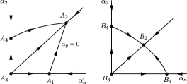
In Fig. 1, we show the schematic phase diagram of model A and the interplay between the UV fixed point FP3 – FP7 (denoted as – ) in more detail (see also Tab. 2). Trajectories are projected onto the plane and arrows indicate the flow from the UV to the IR. is the most relevant UV fixed point. The separatrices responsible for the cross-over from to , from to , or from to relate to the lines , , or , respectively. is the least ultraviolet point only exhibiting as a relevant coupling.
Next, we confirm that some of the UV fixed points in Tab. 2 can be matched onto the SM. Here, it is worth noting that many renormalization group trajectories are attracted by the fully attractive IR fixed point GY2κ, corresponding to FP3 in Tab. 2. If so, the gauge coupling remains too large to be matched against the SM. In other words, UV initial conditions within the basin of attraction of FP3 cannot be matched onto the SM. In concrete terms, this is the case for any trajectory running out of the fixed point or (see Fig. 2 for an example). On the other hand, provided that the gauge coupling takes sufficiently small values in the vicinity of the UV fixed point, trajectories can avoid the FP3. This is the case for both UV fixed points and . Starting from these, remains sufficiently small throughout the entire RG evolution, and matching against the SM possible at a wide range of matching scales between the TeV and the Planck scale. An example for this is shown in Fig. 3.
| Model B | rel. | irrel. | Info | Fig. 1 | Matching | ||||
| FP1 | 0(+) | 0(+) | 0(+) | 0(+) | 0 | 4 | G | ||
| FP2 | 1.953 | 0(-) | 1.562 | 1.888 | 2 | 2 | GY1κy | ✓ | |
| FP3 | 1.224 | 0.186 | 1.326 | 1.541 | 1 | 3 | GY12κy | ✓ | |
| FP4 | 2.712 | 0(-) | 0- | 2.712 | 3 | 1 | GY1y | ✓ | |
| FP5 | 1.732 | 0.216 | 0- | 2.164 | 2 | 2 | GY12y | ✓ |
Finally, it is noteworthy that, unlike in Bond:2017wut ; Kowalska:2017fzw , the Yukawa coupling can be switched off as it is not required to generate the fixed points and . Instead, the Yukawa couplings and are required to enable a fixed point for . Their predicted low energy values are and asuming a matching to ; see Fig. 3.
B Model B (triplets, )
For vector-like fermions the BSM Yukawa Lagrangean takes the form
| (30) |
The components of can be expressed as matrix via:
| (31) |
in accord with the normalization of the kinetic term in equation (2). The upper indices indicate the charge of each component.
We have listed all fixed points of model B in Tab. 3. In this model, the one-loop coefficients of both gauge coupling obey , turning the Gaussian into a total IR fixed point, and prohibiting any kind of Banks-Zaks solutions. Moreover, all gauge-Yukawa fixed points only involving (GY2κ, GY2y, GY2κy) are unphysical, and for the remaining ones, is required, additionally excluding GY1κ, GY12κ.
This singles out the fixed points as listed in Tab. 3. Similarly to the fixed points of model A, is the least ultraviolet with being the only relevant coupling, are connected to it via a second relevant trajectory, while has three relevant directions. This is shown schematically on the right hand side of Fig. 1. A crucial difference, however, is that no infrared GY fixed points with and are realized in model B. Hence, unlike in model A, UV fixed points solutions with finite are not a priori excluded phenomenologically, though constrained, and the corresponding matching conditions can have solutions. Integrating the RG trajectories which leave the UV fixed point into the direction towards lower energies, we find TeV, as depicted in Fig. 4. Similarly, for the fixed point we find . We learn that asymptotic safety can predict the mass scale of new physics. The scale is disfavored phenomenologically, though only narrowly. The impact of higher loop corrections is studied in the following Sec. IV.
Fixed point solutions with require more detailed analysis, as asymptotic freedom is absent. Although is relevant at the fixed points due to the Yukawa interactions, it may turn irrelevant along a trajectory toward the IR, as become smaller causing to become negative.
C Model C (doublets, )
For model C, the BSM fermions have the representation , which is the same as the one of the SM leptons , leading to the Yukawa interactions
| (32) |
All physical fixed points in the 210 approximation are listed in Tab. 4, and have as an irrelevant coupling. Besides the Gaussian (FP1), one Banks-Zaks (FP2) and four Gauge-Yukawa fixed points in (FP3..6) are realized. Similarly to the arguments used in the discussion of model A, the relation , which holds in model C, see (14) and Sec. A for the RG-coefficients, excludes a solution GY. In addition, there is a line of fixed points with (FP6), that covers three solutions GY, GY2y and GY, and give rise to a marginal coupling. However, no physical gauge-Yukawa fixed point involving exists, and hence there is no candidate UV fixed point provided by model C at lowest loop order.
| Model C | rel. | ir. | Info | |||||
| FP1 | 0(+) | 0(-) | 0(+) | 0(+) | 0(+) | 1 | 4 | G |
| FP2 | 0(+) | 0.038 | 0- | 0- | 0- | 3 | 2 | BZ2 |
| FP3 | 0(+) | 0.039 | 0.020 | 0- | 0- | 2 | 3 | GY2κ |
| FP4 | 0(+) | 0.054 | 0.027 | 0.049 | 0+ | 0 | 5 | GY |
| FP5 | 0(+) | 0.053 | 0.011 | 0- | 0.046 | 1 | 4 | GY2κy |
| FP6 | 0(+) | 0.052 | 0- | 1 | 3 | GY |
D Model D (doublets, )
In model D the BSM Yukawa Lagrangean reads
| (33) |
with . Physical fixed points are listed in Tab. 5, with remarkable small coupling values . All solutions suffer from the triviality problem. Besides the Gaussian, and BZ2, all three possible Gauge-Yukawa fixed points involving only are realized (FP3..5 in Tab. 5), but fall in this category. Viable candidates for UV fixed points are of the Gauge-Yukawa type involving at least the gauge coupling as well as the BSM Yukawa interaction , as only GY1κ and GY12κ are unphysical.
Projecting onto the --plane, the hierarchy is similar to model A, see Fig. 1, with being the most, and the least ultraviolet fixed points. Moreover, the same argument holds regarding the total IR fixed point GY2κy, which attracts trajectories going towards SM coupling values like those following the critical direction from , as depicted on the left hand side in Fig. 5. Small values of along the trajectory are required, implying solutions as possible UV fixed points. Matching onto the SM is then possible at a range of scales, for we obtain , which is shown in Fig. 5. Fixed point has also been studied in Barducci:2018ysr , but discarded after including higher order contributions. We retain this fixed point solution, deferring the discussion of higher loop-order effects to Sec. IV.
| Model D | rel. | irrel. | Info | Name | Matching | ||||
| FP1 | 0(+) | 0(-) | 0(+) | 0(+) | 1 | 3 | G | ||
| FP2 | 0(+) | 0.038 | 0- | 0- | 2 | 2 | BZ2 | ||
| FP3 | 0(+) | 0.039 | 0.020 | 0- | 1 | 3 | GY2κ | ||
| FP4 | 0(+) | 0.052 | 0- | 0.047 | 1 | 3 | GY2y | ||
| FP5 | 0(+) | 0.053 | 0.011 | 0.046 | 0 | 4 | GY2κy | ||
| FP6 | 0.246 | 0(-) | 0.322 | 0.631 | 2 | 2 | GY1κy | ✓ | |
| FP7 | 0.202 | 0.145 | 0.295 | 0.647 | 1 | 3 | GY12κy | ✗ | |
| FP8 | 0.288 | 0(-) | 0- | 0.778 | 3 | 1 | GY1y | ✓ | |
| FP9 | 0.239 | 0.152 | 0- | 0.782 | 2 | 2 | GY12y | ✗ |
E Model E (singlets, )
The Yukawa interactions in model E read
| (34) |
Since is a singlet under all gauge groups, is always positive in the 210 approximation, requiring at all scales, as this coupling is irrelevant. This decouples the left-chiral BSM fermion and the BSM scalar from the SM plus at this loop order. Only the Gaussian fixed point, the Banks-Zaks in and a gauge-Yukawa GY2κ are present, and is irrelevant for all of them. This leaves the model without viable candidates of UV fixed points at 210 approximation.
F Model F (triplets, )
In model F, the BSM fermions are in the adjoint of with vanishing hypercharge. The BSM Yukawa sector can be written as
| (35) |
In this setup, asymptotic freedom is absent for both gauge couplings, making the Gaussian completely IR attractive and excluding any kind of Banks-Zaks fixed points. In the 210 approximation, is independent of , and is independent of , as does not carry hypercharge. Hence the two-loop contributions of are the only negative terms in , requiring . Moreover, only contributions are negative in , which suggests that implies and irrelevant. However, none of the remaining gauge-Yukawa solutions GY1κ, GY2κ, GY2κy, GY12κ and GY12κy are realized, as contributions in are too small compared to one and other two loop terms. This leaves the Gaussian as the only physical fixed point; we conclude that there is no AS fixed point at 210 in model F.
G Summary Top-Down
In Secs. A-F we have gained first insights into the fixed point structure of models A – F in a top-down approach of solving the RGEs at leading orders directly, and running towards infrared scales. The results for model A,B and D collected in Tables 2, 3 and 5 show several signatures of UV fixed points that can be matched onto the SM, but also indicate that those are borderline perturbative. This suggests that the fixed points are sensitive to contributions from higher loop orders. We also found that the models C, E and F do not provide any viable solutions at 210 and the question arises whether this is just a feature of the approximation. In order to address both points, we go in Sec. IV beyond the 210 approximation. To handle the increased algebraic complexity of higher loop corrections and the quartic sector, a bottom-up approach will be employed, studying the RG running from the IR to the UV instead, mapping out the BSM critical surface.
IV Running Couplings
In this section, we discuss the renormalization group flow of couplings beyond the leading order approximation which has been employed in the previous Sec. III. We explore in detail how the running of couplings depends on the values of BSM couplings at the matching scale. The main new technical additions in this section are the quartic scalar and the portal couplings, and the inclusion of loop effects up to the complete 2-loop order (222 approximation), or, if available, the complete 3-loop order (333 approximation). We are particularly interested in the running of couplings from a bottom-up perspective, and study the flow for a given set of BSM initial values at the matching scale. We then ask whether these values together with the SM input reach Planckian energies without developing poles, exhibit asymptotic safety, and the stability of the quantum vacuum.
We give our setup and initial conditions in Sec. A, and briefly review the RG-flow within the SM in Sec. B. After identifying relevant correlations between feeble and weakly-sized BSM couplings in Secs C and D, respectively, we present in Sec. E the BSM critical surface for each model.
A Setup and Boundary Conditions
We retain the renormalization group running for the three gauge couplings of the SM (11), and up to three BSM Yukawa couplings (12). Going beyond the leading order 210 approximation, we also retain the Higgs quartic self-interaction , the BSM quartics , and the quartic portal coupling
| (36) |
Moreover, it is well-known that the SM top and bottom Yukawa couplings critically influence the running of the Higgs quartic and, therefore, must be retained as well. We introduce them as
| (37) |
Overall, (11), (12), (36), and (37) results in 12 (or 11) independent running couplings for models A and C (or models B, D, E, and F).
We also remark that the scalar quartic interactions couple back into the Yukawa sectors starting at two loop, and into the gauge sectors starting at three (or four) loop, depending on whether the participating matter fields are charged (uncharged) under the gauge symmetry. Conversely, the Yukawa couplings couple back into the quartic starting at one loop, as do the weak and hypercharge gauge couplings into the Higgs. We expect therefore a crucial interplay between BSM Yukawas and the portal coupling with Higgs stability. In addition, the leading order study in Sec. III showed that some of the fixed point coordinates might come out within the range , indicating that strict perturbativity cannot be guaranteed. For these reasons, we develop the fixed point search and the study of RG equations up to the highest level of approximation where all couplings are treated on an equal footing, the complete two loop order (222 approximation). The running of SM couplings, which serves as a reference scenario, is studied up to the complete three loop order (333 approximation).
All our models require boundary conditions with six SM couplings at the matching scale , which for all practical purposes corresponds to the mass of the BSM fermions . To be specific, we take the matching scale in this section to be
| (38) |
The initial conditions for the SM couplings then read, using GeV and Tanabashi:2018oca ; Buttazzo:2013uya ,
| (39) | ||||||
Hence, in our conventions, initial couplings are within the range . We are now in a position to discuss the running of couplings and the “BSM critical surface”, the set of values for BSM couplings at the matching scale which lead to viable RG trajectories all the way up to the Planck scale.
B Standard Model
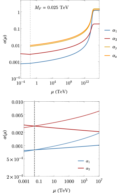
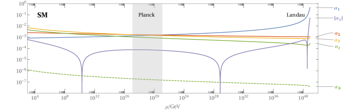
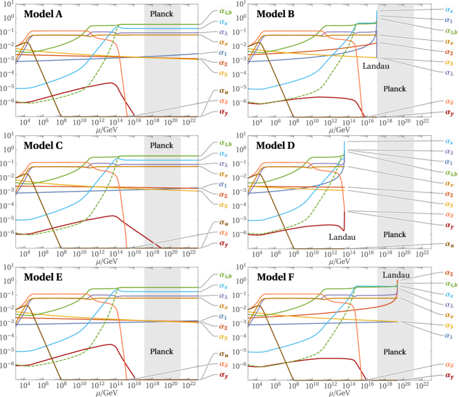
We briefly discuss running couplings within the SM at the complete 3-loop order in perturbation theory Degrassi:2012ry ; Buttazzo:2013uya ; Mihaila:2012fm ; Bednyakov:2012rb ; Bednyakov:2012en ; Bednyakov:2013eba ; Chetyrkin:2012rz ; Chetyrkin:2013wya , displayed in Fig. 6. Overall, the SM running is rather slow with gauge, quartic and Yukawa couplings mostly below or smaller. We also observe that the Higgs potential becomes metastable starting around GeV Degrassi:2012ry ; Buttazzo:2013uya , an effect which is mostly driven by the quantum corrections from the top Yukawa coupling . Further, an imperfect gauge coupling unification is observed around GeV. Quantum gravity is expected to kick in around the Planck scale, GeV, indicated by the gray-shaded area. As an aside, we notice that the Higgs beta function essentially vanishes at Planckian energies
| (40) |
If quantum gravity can be neglected, hypothetically, we may extend the running of couplings into the transplanckian regime. The hypercharge coupling would then reach a Landau pole around GeV. Also, its slow but steady growth would eventually dominate over the slowly decreasing top Yukawa coupling, and thereby stabilize the quantum vacuum starting around GeV. Ultimately, however, the Higgs coupling reaches a Landau pole alongside the coupling and the SM stops being predictive.
C Feeble BSM Couplings
Next, we include new matter fields on top of the SM ones and switch on the BSM couplings at the matching scale (39). A minimally invasive choice are very small, feeble, BSM couplings such that they do not significantly influence the renormalization group flow up to the Planck scale. Their own running would then be well encoded already by the leading order in the perturbative expansion, and models resemble the SM, extended by vector-like fermions. Specifically, we consider here initial values of the order of or smaller.
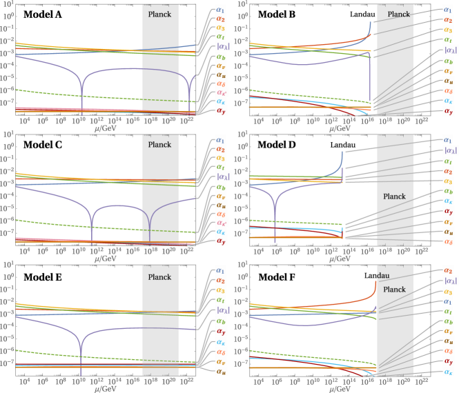
Models A, C, and E
Sample trajectories with feeble BSM couplings are shown in Fig. 7 (plots to the left) for models A, C and E. In all cases, we observe a SM-like running of couplings. The new matter fields modify the running of gauge couplings very mildly. For model A and E, we find a vanishing beta function for the Higgs quartic coupling, much similar to the SM (41). For model C, we observe that the regime of Higgs metastability terminates exactly around the Planck scale,
| (41) |
We conclude that in model A,C and E feeble initial values for the BSM couplings lead to SM-like trajectories including vacuum meta-stability up to the Planck scale. Hence, the BSM critical surface covers the region in which all couplings are feeble.
Models B, D, and F
The models B, D and F with feeble BSM couplings at reach a Landau pole prior to the Planck scale, with sample trajectories shown in Fig. 7 (plots to the right). Specifically, in model B asymptotic freedom for the weak and hypercharge couplings is lost leading to a Landau pole around GeV reached first for the hypercharge, going hand-in-hand with the loss of vacuum stability. Similarly, a strong coupling regime with a Landau pole is reached around GeV (GeV) for model D (model F). Hence, none of these models can make it to the Planck scale for feeble BSM couplings, excluding this region from the BSM critical surface. Notice though that the growth of the gauge couplings in model B and F stabilizes the Higgs sector all the way up to close to the pole.
D Weak BSM Couplings
In the following we explore several matching scenarios for each of the models A – F with BSM couplings of at least the same order of magnitude as the SM couplings at the matching scale (39). In this regime, Yukawa interactions play a crucial role in avoiding Landau poles and stabilizing RG flows, inviting a classification by the couplings involved. Due to the importance for Higgs stability, we also distinguish scenarios with or without portal coupling effects. After identifying relevant correlations between BSM couplings, we obtain in Sec. E the BSM critical surface for each model.
Models A – F with
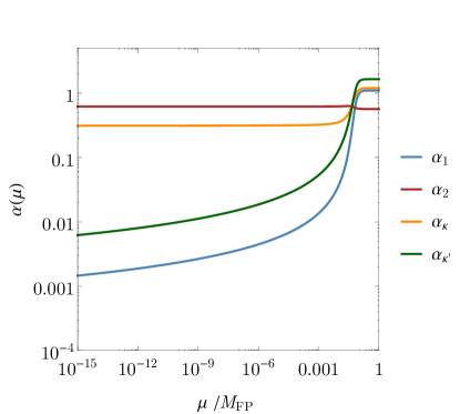
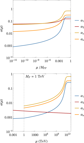
For , the BSM Yukawa slows down the running of gauge couplings and removes all Landau poles before . Moreover, it stabilizes the running of the quartics , due to a walking regime , which may extend until after the Planck scale. This is displayed in Fig. 8. Due to sizable BSM couplings, the portal is being switched on, influencing the running of the Higgs quartic . For larger values , the Higgs potential can be stabilized, i.e., between and (model A and E), while smaller values of cause the Higgs potential to flip sign twice before the Planck scale (model B and F), or remains negative at (model C and D).
In models A, C, D and E, feeble initial values of grow in coupling strength, eventually destabilizing the trajectories in the far UV. For the triplet models B and F, remains small for feeble or weakly coupled , providing greater windows of stability. In summary, the BSM critical surface covers the parameter space where is weak and are feeble at the matching scale.
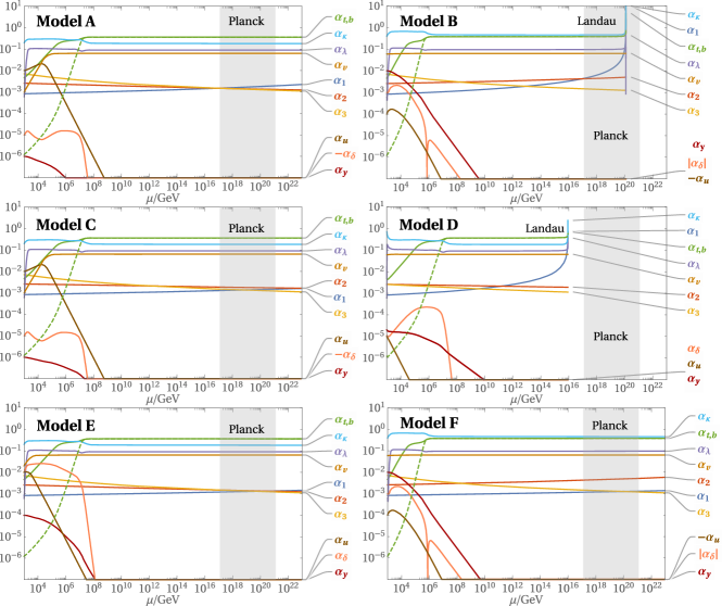
Models A – F with
A weakly coupled Yukawa interaction may stabilize the SM scalar sector. The choice
| (42) |
is depicted in Fig. 9. A common feature of all models A – F is the stabilization of in a walking region together with and the SM Yukawas, as all of which couple to the SM Higgs directly. The BSM potential on the other hand lacks a sizable Yukawa interaction, and self-stabilizes around . This phenomenon is not disrupted by feeble initial values of , which are driven to zero in the UV limit. However, the scenario is not viable for model D as the Landau pole still appears before the Planckian regime. In model B, the pole appears soon after .
The initial value of can be reduced for large enough to stabilize the running of the Higgs quartic:
| (43) |
For models A, C and E, this allows for feeble at the matching scale, while in models B, D and F poles arise below or at the Planck regime, as displayed in Fig. 10.
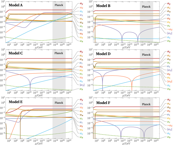
Models A and C with
Models A and C feature the additional Yukawa interaction , giving rise to another walking regime
| (44) |
shown in Fig. 11. Starting from the matching scale , these regions are reached before the Planck scale, and at various speeds by different couplings, creating a rich landscape of intermediate pseudo fixed points and scales. Throughout the walking regime, SM and BSM Yukawas and quartics slow down in model A at
| (45) | ||||||
and in model C at
| (46) | ||||||
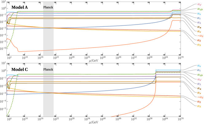
On the other hand, the portal and gauge couplings continue to run, although the latter is slowed down by the magnitude of the Yukawas. Consequently, Landau poles are avoided even far beyond the Planck scale. Moreover, the SM [BSM] quartics are stabilized by the Yukawa couplings. All of these phenomena are consequences of the vicinity of a pseudo-fixed point with , separating the SM and BSM scalar sectors, as well as Yukawa couplings from each other. This decoupling is expected to be realized to all loop-orders, because, in its vicinity, the action decomposes as
| (47) |
for model A [C], up to corrections of the order of the SM lepton Yukawas , (9). However, this separation can only be realized approximately for small gauge and portal couplings. Hence, the RG flow eventually leaves the walking regime in the far UV due to the slow residual running of or . Ultimately, this triggers a cross-over away from the walking regime and into an interacting UV fixed point regime where all couplings bar the non-abelian gauge and the BSM Yukawa couplings take non-trivial values.
Specifically, for model A, the interacting UV fixed point is approximately given by
| (48) | ||||||
Note that the fixed point is rather close to the values of couplings in the walking regime (45). Similarly, in model C we find an approximate UV fixed point with coordinates
| (49) | ||||||
Again, we note that (48) is numerically close to the walking regime (46).
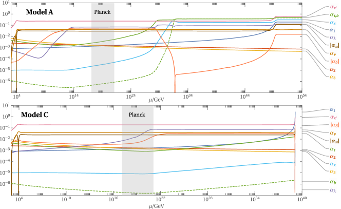
Reducing destabilizes the running of the Higgs self-coupling , which can however be remedied by a non-vanishing portal coupling :
| (50) |
In model A, this enables trajectories with feeble to connect to the phenomena (45) and (48), while for model C, trans-planckian poles arise. This is displayed in Fig. 12. In both models the coupling (brown), whose overall sign separates the vacuum solutions from , (22), changes sign below .
In summary, the BSM critical surfaces of model A and C include regions for both and being perturbartively small. For even smaller values of , larger values of are required, and Higgs stability is not automatically guaranteed. The interplay of BSM input values on Planck-scale features is further detailed below (Sec. E).
We emphasize that our models are the first templates of asymptotically safe SM extensions with physical Higgs, top, and bottom masses, and which connect the relevant SM and BSM couplings at TeV energies with an interacting fixed point at highest energies. Another feature of our models is the low number of new fermion flavors required for this. In contrast, earlier attempts towards asymptotically safe SM extensions Bond:2017wut ; Kowalska:2017fzw ; Mann:2017wzh ; Pelaggi:2017abg required moderate or large , and either neglected the running of quartic and portal couplings Bond:2017wut ; Kowalska:2017fzw , or used an unphysically large mass for the Higgs Mann:2017wzh in large- resummations which require further scrutiny Pelaggi:2017abg ; Alanne:2019vuk . It will therefore be interesting to test the fixed point at higher loop orders, once available, and non-perturbatively using lattice simulations Leino:2019qwk , or functional renormalization.
E BSM Critical Surface
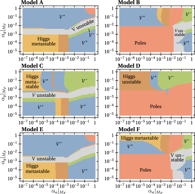
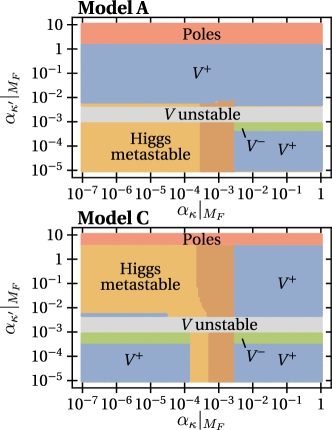
We analyze the state of the vacuum at the Planck scale in dependence on the initial conditions of the BSM couplings at to determine the BSM critical surface in each model. In accord with the reasoning in Sec. D, the BSM Yukawas , are varied at the matching scale, with the SM couplings fixed by (39). The remaining BSM couplings are, exemplarily, set to
| (51) |
For each model, we then sample different initial values and integrate the RG flow at two loop accuracy for all couplings from the matching scale to the Planck scale. The result for all models is shown in Fig. 13. Different parameter regions are color-coded to indicate the type of ground state at the Planck scale, or whether poles or instabilities arise prior to . Specifically, we distinguish regions in that yield stable vacua (blue) or (green), according to (22), evaluated at the Planck scale. Regions with negative Higgs quartic are called metastable (yellow), if , and Higgs-unstable if . In the remaining regions with unstable vacuum (gray) either BSM quartics do not comply with (22) (regardless of and ) or and do comply with (22), but does not. Regions with Landau poles below or at the Planck scale are indicated in red.
Next, we discuss the pattern of results in Fig. 13. Connecting to the region of feeble couplings Fig. 7, Landau poles are present before the Planck scale within at least in models B, D and F. For models A, C and E on the other hand, within no poles arise and the Higgs potential is metastable or even becomes stable at the Planck scale (model C), just as depicted in Fig. 7.
Towards larger values of , models A, C and E exhibit a metastable and then unstable Higgs potential until is large enough to stabilize the potential as in Fig. 9. The vacuum configuration at is then the same as at the matching scale, either or . For models B and F, is required to move the Landau pole past the Planck scale, while this is not possible in model D.
If we are increasing instead, this leads eventually to the ground state in the BSM potential, but Higgs stability is not guaranteed automatically, see Fig. 8. If not obstructed by poles, each model exhibits a narrow ”belt” of parameters around and any , within which the BSM potential is unstable due to in the ground state. Here, Coleman-Weinberg resummations Litim:2015iea or higher order scalar selfinteractions Buyukbese:2017ehm should be included before definite conclusions about stability are taken.
Another feature of models A and E is that for simultaneously, Landau poles occur before the Planck scale. For the other models, RG trajectories are stabilized around in the ground state by quartic interactions. However, this region is especially sensitive to corrections from higher loop orders.
For models A and C, the additional Yukawa interaction adds an extra dimension to the BSM critical surface. Its impact is further investigated in Fig. 14 (color-coding as in Fig. 13) where we exemplarily explore the vacuum state at the Planck scale within the parameter plane, and
| (52) |
We find that the region with is very similar to the region in Fig. 13, featuring a stable ground state for weakly coupled . For both the phenomena illustrated in Fig. 11 occur, implying a stable region. The fate of the quadrant with and hinges on the value of . As can be seen from Fig. 14, its flow can be stable, as in Fig. 12, while poles or Higgs metastability are possible as well.
The BSM critical surface at the matching scale of each model consists of the combined plus regions, with slices in the multi-dimensional parameter space shown in Fig. 13 and Fig. 14 in green and blue. All models A – F can be stable at least up to the Planck scale. The yellow (metastability) regions may be included as well, as this corresponds to the situation of the SM. In general, experimental constraints on the BSM critical surface apply for matching scales around the TeV-scale, a topic further discussed in the next Sec. V.
V Phenomenology
In this section, we investigate the phenomenological implications of our models. Specifically, in Sec. A we discuss BSM sector production at hadron and lepton colliders, and in Sec. B the decays of the BSM fermions and scalar. An important ingredient for phenomenology is mixing between SM and BSM fermions, the technical details for which are relegated to App. D. Resulting phenomenological consequences are worked out in Sec. C and include dileptonic decays of the scalars. Constraints from Drell-Yan data on the matching scale are worked out in Sec. D. Implications for the leptons’ anomalous magnetic moments are studied in Sec. E. In Sec. F we show that the portal coupling in (21) together with and can provide a chirally enhanced contribution to the magnetic moments. This mechanism also induces EDMs for CP-violating couplings, discussed in Sec. G. In Sec. H we discuss constraints from charged lepton flavor violating (LFV) decays.
A BSM Sector Production
Tree-level production channels of the BSM sector at or colliders are shown in Fig. 15. Since the fermions are colorless, pair production in collisions is limited to quark-antiquark fusion to electroweak gauge bosons (diagrams (a) and (b)). Single production through Yukawa interactions with -channel Higgs (diagram (c)) is also possible. In colliders, the can also be produced with -channel Higgs or in pairs (d) and singly (e). The contribution to production from -channel neutral bosons is especially relevant, since it is present in all models in study (except for model E), in both and collisions, and all flavors of are produced. In the limit , where is a quark or a lepton and denotes its mass (charge), the contribution to pair production via photon exchange at center of mass energy-squared reads
| (53) |
where we summed over the ’s flavors and -components; denotes the fine structure constant. Corresponding cross sections are of the order Patrignani:2016xqp . Note the enhancement in model B and D which contain fermions with , and result in effective charge-squares of .

The BSM scalars, which are SM singlets, can be pair-produced at lepton colliders in model A and C through the Yukawa interactions with -exchange (diagram (f)). The cross-section, for , then reads
| (54) |
Denote by and the real, CP-even and CP-odd physical degrees of freedom of , respectively. Together the Yukawas and induce single -production, or , in association with a Higgs (diagram (f)).
Another mechanism to probe the scalars is through -Higgs mixing (diagram (g)), which arises if the portal coupling is switched on. In this diagram, the and couplings arise after electroweak symmetry breaking. In addition, the vertex is possible when the scalar acquires a VEV. A detailed study of production at colliders is, however, beyond the scope of this work.
B BSM Sector Decay
We discuss, in this order, the decays of the vector-like leptons and the BSM scalar . Both subsections contain a brief summary at the beginning.
Fermions
Depending on the representation, coupling and mass hierarchies, the BSM fermions can decay through the Yukawa interactions to Higgs plus lepton or to plus lepton (only model A and C), while some members of the -multiplets need to cascade down within the multiplet first through -exchange. These are the states with electric charge (model B and D) and (model F). As detailed below, they allow for macroscopic lifetimes. Mixing with the SM leptons induces additional -decays to plus lepton which are discussed in Sec. C.
The vector-like fermions with and can decay through the Yukawa interactions to and , respectively, except in model C, in which the Higgs couples to -singlet leptons and only the decay takes place through . Neglecting the lepton mass, the decay rate into Higgs plus lepton is
| (55) |
where for the states in models B,F and otherwise. For and at least a TeV, one obtains a lifetime s, which leads to a prompt decay. In models A (C), the decays () are also allowed if the BSM scalars are lighter than the vector-like fermions, with rate
| (56) |
Models B and D contain fermions. After electroweak symmetry breaking, these cascade down through the weak interaction as , and subsequent decays. The lifetime is then driven by the mass splitting within the multiplet. In the limit one obtains for from SM gauge boson loops Cirelli:2005uq and , , which is around a GeV in both models. Corresponding decay rates indicate around picosecond lifetimes of the , with a small, however macroscopic mm resulting in displaced vertex signatures that can be searched for at the LHC Evans:2016zau . In model F, the fermions decay similarly through , with . Numerically, this is an order of magnitude smaller than the splitting in model B and D and suppresses the decay rate significantly further, allowing for striking long-lived charged particle signatures. Note that the presence of fermion mixing, discussed in the following, can induce more frequent decays unless couplings are very suppressed.
Note the upper limit on general mass splittings within the fermion -multiplets by the -parameter Patrignani:2016xqp
| (57) |
where is the Dynkin index of the representation of (see Bond:2017wut for details). Specifically, for models A and E, models C and D, and models B and F, respectively. The allowed splitting is hence about a few percent for TeV-ish fermion masses.
Scalars
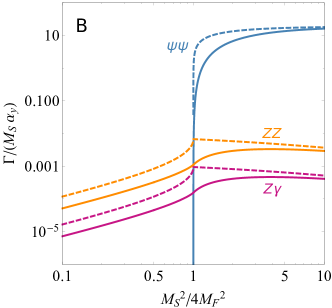
If kinematically allowed, the scalars decay in all models through Yukawa couplings to , and in model A and C to plus lepton. Only the flavor diagonal components can, except in the SM-singlet model E, in addition decay to electroweak gauge bosons through the -Yukawa and a triangle loop with ’s, , with . Mixing of the vector-like fermions with the SM leptons induces BSM scalar decays to dileptons, further discussed in Sec. C.
For decays to vector-like fermions and leptons through the mixed Yukawas , i.e., in model A and C, are kinematically open. In all models, the decay to is possible for through the Yukawa coupling . Only the flavor diagonal components of can decay in this manner. The tree-level decay rates for a given flavor-specific component can be written as
| (58) | ||||
where model-dependent multiplicities in the final states are not spelled out explicitly. For instance, in model B, decays to plus CP conjugate ones. The loop-induced decays to gauge bosons read
| (59) |
where the coefficients depend on the representation of and in the limit can be expressed as
| (60) | ||||
In (58), (59), and correspond to the scalar and pseudoscalar parts of , respectively, and with
| (61) |
and Gunion:1989we . In the case of one of the mixing with angle with the Higgs, the real part of can decay through mixing with rate , where is the decay rate of the Higgs in the SM.
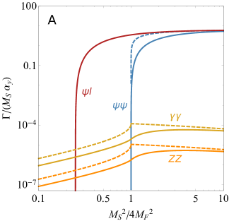
In model A the main decay channels are and , followed by the decay to photons. Other gauge boson modes are further suppressed, as for holds . The reduced rates as a function of for model A are shown in Fig. 16 for .
In model B,C, D and F the vector-like fermions are charged under , and allow for decays to . When kinematically allowed, the tree-level decays into are dominant. For model B this is shown in Fig. 17. The hierarchy between the gauge boson decay rates in model B reads , and in model C . In model D, the hierarchies are , whereas in model F .
For and negligible one may wonder whether can decay at all. However, fermion mixing induces decays to SM leptons or neutrinos, discussed next.
| Vacuum | ||||||
| 0 |
C Fermion Mixing
Mixing between SM leptons and BSM fermions provides relevant phenomenology. Mixing angles – in the small angle approximation to make the parametric dependence explicit – for the left-handed and right-handed fermions, with the model M indicated as superscript, are given in Table 6. Details are given in App. D. We discuss, in this order, the impact of mixing on scalar decays, modified electroweak and Higgs couplings and decays of vector-like leptons to SM lepton. The results are important for experimental searches because they imply that all and eventually decay to SM leptons, charged ones and neutrinos, with the only exceptions being the diagonal decays.
LFV-like Scalar Decay
In models A and C, mixing induces tree-level decays at the order , using the angles of Tab. 11. These can be competitive with decays to electroweak bosons: for instance, taking and for of order or larger they dominate over in model A. Unless the mixing is strongly suppressed, for at the TeV scale, the lifetime is below picoseconds, and too short for a macroscopic decay length.
In models B, D and F, for , fermion mixing induces the decays (models B and F) and (model D) at the order . For , the decays at the order are the leading ones. Using (58) again, one obtains a lifetime of picoseconds or above for a suppression factor . Due to its flavor dependence, the suppression of the mixing is stronger for tau-less final states. This could allow for displaced decays into dielectrons, dimuons and , while at the same time, those into ditaus, and could remain prompt.
Lastly, for models with fermion decays are also allowed for , occurring at order for models B, E and F and at order for model C. In the case of model E, this is the only available decay mode of the off-diagonal (apart from if allowed), leading to below-picosecond lifetimes for . Study of the different decay modes into various gauge bosons or fermions can be used for experimental discrimination of models. The patterns of final state leptons in LFV-like 222Despite the different lepton flavors in the final state processes such as are, strictly speaking, LFV-like only because flavor is conserved in the decay. decays, , or can help to understand hierarchies.
Impact on and Higgs Couplings
Fermion mixing gives rise to tree-level effects in the couplings of leptons and vector-like fermions to the massive electroweak bosons. In the case of the couplings to two leptons, the Lagrangean in the fermion mass basis acquires couplings
| (62) |
with respect to their SM values and , and where is the isospin of the component of the vector-like fermions in each model. The rotation angles are to be taken from Tab. (6) according to the chosen vacuum structure and the lepton flavor . In the case of model A (C), one finds (), yielding modifications purely proportional to (). In models B, E and F one finds , while model D presents , so that in all models the present modifications proportional to . In models with fermions (B, C, E and F), the couplings to two neutrinos become
| (63) |
with . In model C, for which , remains unaffected. Therefore, in all models data mainly constrains the mixing angles proportional to . Measurements of the couplings to charged leptons and the electron-flavored neutrinos demand or smaller Tanabashi:2018oca , which implies
| (64) |
Modifications of the couplings remain also in agreement with decay measurement if (64) is fulfilled (see appendix E for details). Additionally, Higgs couplings are modified by mixing as well. Since charged leptons acquire mass from several Yukawa interactions, the couplings of in the mass basis fulfil
| (65) |
for model A, while replacing gives the expression for model C. In all other models, the term is absent. For angles fulfilling vertex constraints according to Eq. (64), Higgs signal strength bounds are avoidable for all leptons Tanabashi:2018oca ; Altmannshofer:2015qra .
Electroweak Decays of Vector-like Leptons
Finally, mixing induces decays of the vector-like fermions to weak bosons and leptons at tree-level, with rates
| (66) | ||||
where , , , and the coefficients and are collected in Tab. 10 and Tab. 11 respectively for all models. Let us discuss the decays of the chargeless in model C, which occur exclusively through its mixing unless via is allowed. For the universal vacuum and for the flavor in which the flavor-specific vacuum points, it is important to note that the is lighter than the by GeV. This difference causes isospin-breaking in the mixing angles given in Table 6, which induces a CKM-like misalignment between up and down sectors , such that the decay can take place. Assuming , we estimate . Unless , the decays faster than picoseconds.
For the flavors in the lepton-specific vacuum which do not get a corresponding VEV in , the left- and right-handed angles have the opposite hierarchy, fulfilling . Since , the decay promptly through with .
D Drell-Yan
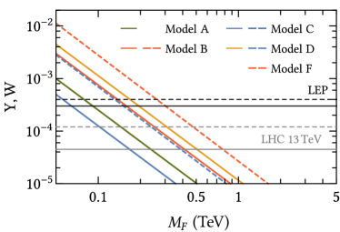
Modifications of the running of the electroweak couplings can be constrained directly from charged and neutral current Drell-Yan processes. Of particular interest are the electroweak precision parameters and , which are linearly dependent on the BSM contribution to the running of and respectively as Alves:2014cda
| (67) |
where and . A lower limit on the mass of the vector-like fermions can be directly extracted from experimental bounds on Farina:2016rws . As shown in Fig. 18, these require TeV for model A and TeV for models B, C respectively. In models D, F one obtains respectively, while in model E one cannot extract bounds due to the BSM sector being uncharged under the SM gauge symmetries. The bound for model B excludes fixed points and , which can only be matched at TeV. Remarkably, the fixed points that remain viable in terms of matching are only those which present a free . The effect of two-loop corrections in may be estimated by taking the effective coefficients instead of in (67). In our matching scenarios, this typically induces relative changes of order or less in with respect to the one-loop values, and remain positive. The smallness of these corrections is due to the fact that all couplings at low scales present values of order , which are suppressing the two-loop effects, while are typically of order 1 or larger.
E Anomalous Magnetic Moments
The measurements of the electron and muon anomalous magnetic moments are in tension with SM predictions, offering hints for new physics. In the case of the muon, the long-standing discrepancy amounts to Tanabashi:2018oca
| (68) |
Adding uncertainties in quadrature, this represents a deviation from the SM, while recent theory predictions find up to Jegerlehner:2017lbd ; Davier:2016iru .333The possibility of rendering insignificant has recently been suggested by a lattice determination of the hadronic vacuum polarization Borsanyi:2020mff . Further scrutiny is required Aoyama:2020ynm due to tensions with electroweak data Crivellin:2020zul ; Keshavarzi:2020bfy and earlier lattice studies. For the magnetic moment of the electron, recent measurements lead to
| (69) |
corresponding to a pull of from the SM prediction Hanneke:2008tm ; Parker:2018vye .
From a model building perspective it is important to understand which new physics ingredients are required to explain the anomalies (68), (69) simultaneously. Given that the electron and muon deviations point into opposite directions, it is commonly assumed that an explanation requires the manifest breaking of lepton flavor universality. BSM models which explain both anomalies by giving up on lepton flavor universality have used either new light scalar fields Davoudiasl:2018fbb ; Liu:2018xkx ; Gardner:2019mcl ; Cornella:2019uxs ; Bauer:2019gfk ; Dutta:2020scq , supersymmetry Dutta:2018fge ; Endo:2019bcj ; Badziak:2019gaf ; Yang:2020bmh , bottom-up models Crivellin:2018qmi ; Crivellin:2019mvj , leptoquarks Bigaran:2020jil ; Dorsner:2020aaz , two-Higgs doublet models Botella:2020xzf ; Jana:2020pxx , or other BSM mechanisms which treat electrons and muons manifestly differently Han:2018znu ; Abdullah:2019ofw ; CarcamoHernandez:2020pxw ; Haba:2020gkr ; Calibbi:2020emz ; Arbelaez:2020rbq ; Chen:2020jvl ; Hati:2020fzp ; Jana:2020joi . In the spirit of Occam’s razor, however, we have shown recently that the data can very well be explained without any manifest breaking of lepton universality Hiller:2019mou , which is in marked contrast to any of the alternative explanations offered by Davoudiasl:2018fbb ; Liu:2018xkx ; Gardner:2019mcl ; Cornella:2019uxs ; Bauer:2019gfk ; Dutta:2020scq ; Dutta:2018fge ; Endo:2019bcj ; Badziak:2019gaf ; Yang:2020bmh ; Crivellin:2018qmi ; Crivellin:2019mvj ; Bigaran:2020jil ; Dorsner:2020aaz ; Botella:2020xzf ; Jana:2020pxx ; Han:2018znu ; Abdullah:2019ofw ; CarcamoHernandez:2020pxw ; Haba:2020gkr ; Calibbi:2020emz ; Arbelaez:2020rbq ; Chen:2020jvl ; Hati:2020fzp .
In this and the following subsection, we detail how the models A, B, C, D, and F induce anomalous magnetic moments at one-loop, and why, ultimately, only models A and C can explain the present data. Note that model E does not appear in the list, the reason being that the charged SM leptons do no longer couple to BSM fermions after electroweak symmetry breaking. The setting previously put forward by us in Hiller:2019mou corresponds to model A and model C of the present paper.
Specifically, new physics contributions to arise through the 1-loop diagrams shown in Fig. 19. In the limit where is much larger than the mass of the lepton and the scalar propagating in the loop, the NP contribution typically scales as
| (70) |
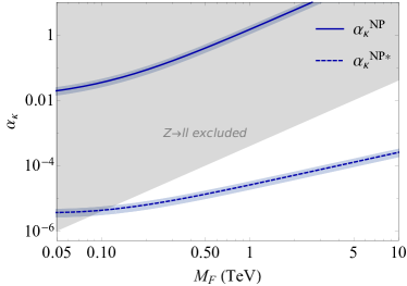
where denotes the lepton mass and is one of the mixed Yukawa couplings; see appendix B for details. For couplings of comparable order, the largest contribution comes from the latter, which couples the vector-like fermions to the lighter scalar (the Higgs). The parameter space compatible with (68) is shown in Fig. 20. As obvious from (B.2), (70) is manifestly positive, and cannot account for . For the muon anomaly (68), the coupling in model A, C and D as well as for model B and F is required. This is however ruled out by the constraint (64). We learn that the models B, D, E and F cannot accommodate either of the present data (68), (69). Models A and C on the other hand have an additional diagram from exchange, Fig. 19b). In fact, since the field is a matrix in flavor space the unobserved flavor index of the BSM fermion in the loop makes this in total contributions. The external chirality flip again induces a contribution quadratic in lepton mass (70) which can account for , since the coupling to the scalar singlet is much less constrained than the one to the Higgs Hiller:2019mou .


Certain NP scenarios, notably supersymmetric ones, can evade one power of lepton mass suppression in (70) by having instead the requisite chiral flip on the heavy fermion line in the loop, as in Fig 21, such that
| (71) |
opening up the possibility for larger contributions to , and dipole operators in general. For we explore this further for models A and C in Sec. F. Another application are electric dipole moments, discussed in Sec. G.
F Scalar Mixing and Chiral Enhancement
The scalar potential involving the SM and BSM scalars and and the various quartic couplings and scalar mass terms has been given in (21). To investigate the prospect of chiral enhancement for dipole operators, such as those responsible for , EDMs, or , we need to investigate the ground states. Using the methods of Litim:2015iea ; Paterson:1980fc two ground states have been identified in (22), including the conditions for couplings. The ground state respects flavor universality in interactions with the SM because it breaks due to the diagonal VEV . Conversely, spontaneously violates flavor universality because it breaks to by only allowing a single diagonal component to pick up a non-vanishing VEV .
If both scalars and acquire a VEV, the portal coupling induces a non-diagonal mass term in the potential which allows the scalars to mix. Together with both BSM Yukawas , chiral enhancement can occur in models A and C. A corresponding contribution to is shown in Fig. 21. Firstly, we study the case , where a single diagonal component of generates a VEV. The component is chosen in order to target the generation of leptons in the term . We define
| (72) |
The mass matrix of the entire scalar sector is diagonal except for the mixing of and . Concentrating on this sub-system, the mass eigenstates can be expressed in terms of the mixing angle as
| (73) |
where
| (74) |
see App. D for details. Neglecting for the sake of this discussion the mixing induced by the scalar VEVs in the fermion system, the BSM Yukawa Lagrangean in the scalar mass basis reads
| (75) | ||||
where we have again assumed real and . Provided that the mass eigenstate is much heavier than and , and in the limit the leading contribution to reads, for with ,
| (76) |
see App. B for details. This contribution is switched on only when both left and right chiral couplings of the lepton to the same scalar are present, a condition which is met by scalar mixing, and which comes with an enhancement factor with respect to NP contributions such as (70). can have either sign.
If the vacuum is aligned in the muon direction, benefits from chiral enhancement (76). Fig. 22 shows for which values of the contribution to equals (68) for some benchmark values of . Also shown is an upper limit on the mixing angle from Higgs signal strength measurements Patrignani:2016xqp .
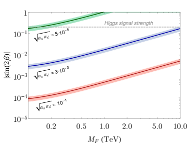
Next we consider the case , where the BSM VEV is universal in all flavors. Here mixing occurs between the and the three states acquiring the VEV. However, two of the mass eigenstates contain no component in the direction, and thus only mix the states within themselves. The two normalized mass eigenstates which have non-vanishing components in the direction are
| (77) | ||||
Hence, the mixing pattern with is identical for all . The enhanced contribution to the anomalous magnetic moments affects all lepton generations, and reads
| (78) |
As , it can a priori have either sign, and can accommodate future data by adjusting together with the quartics. The parameter space that fits is, up to a factor , the same as for , shown in Fig. 22, and we note that this factor cancels with the one for the angle , which obeys
| (79) |
for and , see App. D for details.
Owing to (78), we emphasize that fixing the parameter in to explain in (68) also induces a contribution to the anomalous magnetic moments of the electron and the tau,
| (80) | |||||
| (81) |
The former, however, is in conflict with the data for in (69), both in magnitude and in sign, while the latter is four orders of magnitude away from present limits on Tanabashi:2018oca .
On the other hand, larger couplings allow for a simultaneous explanation of both data points (68) and (69). This mechanism uses the diagrams in Fig. 19b) to generate , and the chirally enhanced diagram of Fig. 21 to generate , without introducing flavor structure explicitly, and irrespective of the vacuum being flavor blind or electron-aligned with ). Moreover, the underlying mechanism is not fine-tuned and could, in principle, accommodate a wide range of deviations and different from present data.
Since the underlying Lagrangean does not break lepton flavor, this mechanism leads additionally to a prediction for the deviations of the tau anomalous magnetic moment . Using the data (68) and (69), our models predict
| (82) |
if the vacuum is flavor-blind, or
| (83) |
if the ground state is electron-aligned, respectively. Further details of this scenario can be found in Hiller:2019mou .
G EDMs
Unlike in the remainder of this work, here we allow the BSM Yukawas to be complex-valued. If the portal interaction is present, in models A and C a relative phase between and induces an Electric Dipole Moment (EDM) of the SM leptons through the chirally enhanced 1-loop diagram Fig. 21. The EDM-Lagrangean can be written as
| (84) |
where denotes the electromagnetic field strength tensor and the lepton electric dipole moment with mass dimension .
For model A, and in the large- limit, we find
| (85) |
where the flavor-specific vacuum is assumed with denoting the flavor distinguished by the ground state . Here, an EDM arises solely for the lepton flavor selected spontaneously by the vacuum. In turn, assuming the vacuum and provided that the CP-phases are lepton-universal, we find instead
| (86) |
for any flavor, and all EDMs are predicted to be equal. The same expressions (85), (86) and results hold true for model C except for the replacement .
The current experimental bounds on and
| (87) | ||||
by the ACME and Muon g-2 collaborations @90 % CL Andreev:2018ayy ; Bennett:2008dy respectively, imply the bound
| (88) |
from the electron data, while the bound from muons is ten orders of magnitude weaker. Comparing this to (68) induced by the same mechanism, see Fig. 22, the CP-phases must be suppressed at the order (-bound) and are unsuppressed by the muon EDM data. If the lepton EDMs are induced by a lepton flavor nonuniversal mechanism, flavor-dependent CP-phases or in a vacuum pointing in the muon direction, the electron EDM bound could be bypassed and the muon EDM could be as large as given (68) with order one phases. Interestingly, this is in reach of future experiments Crivellin:2018qmi .
H Charged LFV Processes
In the setup with Yukawa interactions (3), (7) and (8) flavor is conserved. While there is intergenerational mixing in Yukawas with , no charged LFV proper occurs, see footnote 2. Here we envision a situation beyond (8) and allow for additional flavor off-diagonal couplings. Our aim is to see whether and how well such variants can be probed in LFV processes.
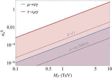
The decay rate induced by a Higgs-fermion loop in all models except the singlet model E for and can be written as Lavoura:2003xp
| (89) |
with
| (90) |
where corresponds to the flavors of the BSM fermion in the loop, see appendix C for details. In (90), a flavor pattern proportional to plus small off-diagonal entries of the order is assumed that is responsible for charged LFV. Hence, , and arises at order . Fig. 23 shows how present bounds Tanabashi:2018oca
| (91) |
at 90% CL and projected bounds from the MEG-II experiment Cavoto:2017kub constrain depending on . Also shown for comparison is the constraint on diagonal couplings from -data (64). While present constraints on the off-diagonal entry (blue) are comparable to the diagonal ones from , the ones on and (red) are significantly weaker.
LFV decays into three lepton final states are also possible, receiving contributions from both penguin and box diagrams with . We estimate Chowdhury:2018nhd
| (92) |
which is -suppressed as (89). Present bounds from the SINDRUM collaboration Bellgardt:1987du give . This is indeed comparable with bounds in Fig. 23, yet not more excluding. The parameter space will be further probed by the Mu3e experiment, which aims at a reach of Perrevoort:2018cqi . For decays to three charged leptons, present bounds pose loose constraints on off-diagonal couplings, .
On the other hand, to conversion processes have a limit in gold nuclei on the conversion rate (CR) of CR at 90% CL by the SINDRUM II collaboration Bertl:2006up . In our models the conversion process is possible through and penguin contributions which receive suppression. We estimate CR Kitano:2002mt , in close competition with bounds. The future Mu2e experiment DonghiaonbehalfoftheMu2eCalorimeterGroup:2017aei , with expected sensitivity CR, can improve the bound from SINDRUM II on by about two orders of magnitude.
Along the lines of the anomalous magnetic moments, scalar mixing induces chirally enhanced contributions to LFV dipole operators if contains non-vanishing off-diagonal elements. For instance, the rate for becomes
| (93) |
in the same approximations as in (76) and pointing in the muon direction. (There is a similar contribution induced by which requires a scalar VEV in the electron direction.) Constraints on from the chirally enhanced amplitude are stronger than on by a factor .
VI Conclusions
We have studied SM extensions with three generations of vector-like leptons and a new singlet matrix scalar field, inspired by asymptotic safety. The main focus has been on new physics implications for settings where the running couplings remain finite and well-defined at least up to the Planck scale, and possibly beyond. A key novelty over earlier models are Higgs and flavor portals (Tab. 1) which are explored in depth. Within this setup we show that the number of new fermion generations required for asymptotically safe or Planck safe extensions can be much lower than thought previously.
Using the renormalization group, we have provided a comprehensive study of six basic models. All of them are found to be well-behaved up to the Planck scale in certain parameter regimes, owing to Yukawa couplings linking SM and BSM fermions with the Higgs (Figs. 7 – 10). The TeV scale initial conditions for BSM couplings (Fig. 13) illustrate parameter regions which do not run into Landau poles and vacuum instabilities or metastabilities. Similar results are found for models which admit a secondary Yukawa coupling between SM and BSM fermions and the new scalars (Figs. 11, 12) with a corresponding critical surface of parameters (Fig. 14). Very explicitly we learn that the requirement for safety up to the Planck scale provides a testable selection criterion in the BSM parameter space.
A conceptual novelty is the use of both ”top-down” and ”bottom-up” searches to find fixed points and Planck safe parameter regions. On the technical side, we have retained the RGEs for the gauge, Yukawa, and quartic couplings up to the complete two loop order, extending upon previous studies. New features are walking regimes, and new patterns for fixed points due to a competition between Yukawa, portal, and gauge couplings. Theories where the running of couplings can be extended to infinite energy are of interest in their own right. Our asymptotically safe extensions are the first ones which achieve this for the key SM and BSM couplings, and in accord with the measured values of the gauge couplings and the Higgs, top, and bottom masses.
Our models also offer a rich phenomenology due to their close ties with the SM through Yukawa and Higgs portals. Genuine features are LFV-like signatures in scalar decays
also with displaced vertices for sufficiently small coupling. The vector-like leptons can have exotic charges which can lead to displaced vertex signatures. The models can be experimentally probed at colliders (Fig. 15), specifically through and Drell-Yan production, and additionally, at or machines, through single production Benedikt:2018qee ; Zimmermann:2018wfu . The BSM scalars can be pair-produced at lepton colliders, or in , if portal effects are present. It would be interesting to check whether existing new physics searches at the LHC in lepton-rich final states lead to constraints on model parameters. As no dedicated analysis for the models here has been performed, however, this requires a re-interpretation of existing searches which is beyond the scope of this work.
Finally, we comment on outstanding features related to lepton universality and low energy probes for new physics, i.e. measurements of the lepton’s magnetic or electric dipole moments. Except for the breaking by SM Yukawas, lepton universality is manifest in all our models and may or may not be broken spontaneously by the vacuum. Irrespective of the ground state, however, we find that two of the six basic models can explain the electron anomaly alone, the muon anomaly alone, or both anomalies together. The latter is rather remarkable in that it also entails a prediction for the tau anomalous magnetic moment Hiller:2019mou , whereas any other BSM explanation of the muon and electron anomalies requires a manifest breaking of lepton universality Davoudiasl:2018fbb ; Liu:2018xkx ; Gardner:2019mcl ; Cornella:2019uxs ; Bauer:2019gfk ; Dutta:2020scq ; Dutta:2018fge ; Endo:2019bcj ; Badziak:2019gaf ; Yang:2020bmh ; Crivellin:2018qmi ; Crivellin:2019mvj ; Bigaran:2020jil ; Dorsner:2020aaz ; Botella:2020xzf ; Jana:2020pxx ; Han:2018znu ; Abdullah:2019ofw ; CarcamoHernandez:2020pxw ; Haba:2020gkr ; Calibbi:2020emz ; Arbelaez:2020rbq ; Chen:2020jvl ; Hati:2020fzp . In addition, provided the vacuum is flavorful and points into the muon direction, we find that the electron EDM bound can be bypassed with a sizeable muon EDM at the level of .
We look forward to further exploration of asymptotically safe model building and searches.
Acknowledgements
GH and DL thank the Aspen Center for Physics, which is supported by National Science Foundation grant PHY-1607611, for hospitality while part of this work was performed. Some results have been presented at the Moriond Electroweak conference 2019 and at the workshop ”Asymptotic Safety meets Particle Physics” (Dortmund 2019). This work has been supported by the DFG Research Unit FOR 1873 “Quark Flavor Physics and Effective Field Theories”.
Appendices
The following appendices collect technical details and useful formulæ used within the main manuscript.
A Two Loop -functions
In this appendix, we detail -functions for the models A – F up to two-loop order. The results are based on Machacek:1983tz ; Machacek:1983fi ; Machacek:1984zw ; Luo:2002ti ; Schienbein:2018fsw ; Pickering:2001aq ; Mihaila:2012pz .
| Model | ||||||||||||||||
| A | 15 | 36 | 3 | 0 | 6 | 6 | 2 | 8 | 9 | 15/2 | 9/2 | 8 | 8 | 0 | 12 | 0 |
| B | 45/4 | 0 | 33/4 | 0 | 6 | 6 | 1/2 | 0 | 23/4 | 15/2 | 33/2 | |||||
| C | 15 | 18 | 3 | 18 | 9/2 | 9/2 | 1 | 10 | 9 | 15/2 | 9/2 | 10 | 10 | 0 | 3 | 9 |
| D | 39 | 0 | 3 | 0 | 6 | 6 | 1 | 0 | 9 | 39/2 | 9/2 | |||||
| E | 3 | 0 | 3 | 0 | 6 | 6 | 2 | 0 | 9 | 3/2 | 9/2 | |||||
| F | 9/4 | 0 | 33/4 | 0 | 6 | 6 | 1/2 | 0 | 23/4 | 3/2 | 33/2 |
The two-loop gauge and one-loop Yukawa RGEs at can be expressed as
| (A.1) | ||||
corresponding to (13) and (14) in the main text. Some of the loop coefficients are model-specific and listed in Tab. 7, while others are universal or can be expressed in a general way in terms of the representation of the vector-like fermions under and their hypercharge . In what follows, denotes the quadratic Casimir invariant and the Dynkin index (see Bond:2017wut for details).
For the hypercharge coupling, these generic coefficients read
| (A.2) | ||||
For the weak coupling, one obtains
| (A.3) | ||||
Finally, for the strong coupling the coefficients are independent of the BSM sector
| (A.4) | ||||||||
For the Yukawa coefficients, we note that only couples into the one-loop running of the top and bottom Yukawas , see Tab. 7. Further loop coefficients for Yukawa couplings at one loop are given by
| (A.5) | ||||||
In a similar vein, there are no one-loop contributions from to and . For one finds
| (A.6) | ||||
Loop coefficients for which are universal in all models are given by
| (A.7) | ||||
while those which are model specific are summarized in Tab. 7.
For the scalar couplings at one loop, it is convenient to use the definition
| (A.8) |
In this convention, the one loop RGEs for the scalar quartic couplings read
| (A.9) | ||||
Here, denotes the one-loop -function of the Higgs quartic in the SM. The one loop coefficients and are tabulated in Tab. 8.
| Model | |||||||||||
| A | 12 | 6 | 75/4 | 33/2 | 9/4 | 10 | 14 | 12 | 0 | 12 | 0 |
| B | 9 | 15/8 | 225/16 | 51/8 | 21/16 | 47/32 | 39/8 | 15/4 | 15/2 | 9 | 18 |
| C | 12 | 6 | 75/4 | 33/2 | 9/4 | 10 | 16 | 12 | 0 | 6 | 6 |
| D | 12 | 6 | 219/4 | 39/2 | 9/4 | 10 | 16 | 36 | 0 | 30 | 6 |
| E | 12 | 6 | 3/4 | 3/2 | 9/4 | 10 | 14 | 0 | 0 | 0 | 0 |
| F | 9 | 15/8 | 9/16 | 57/8 | -21/16 | 47/32 | 39/8 | 0 | 15/2 | 0 | 18 |
At two-loop order, running of the couplings is modified via
| (A.10) | ||||
using coefficients in Tab. 7,8, and denote the two loop beta functions of the SM.
Finally, the two-loop contributions for the BSM scalar quartics are
| (A.12) | ||||
with model-specific loop coefficients tabulated in Tab. 8.
| Model | |||||||
| A | 19/2 | 24 | 37/4 | 51/4 | 6 | 225/8 | 721/12 |
| B | 57/32 | 59/8 | 37/16 | 101/16 | 6 | 1343/32 | 1249/12 |
| C | 5 | 24 | 55/8 | 33/8 | 15 | 225/8 | 589/12 |
| D | 5 | 24 | 95/8 | 33/8 | 27 | 225/8 | 4541/12 |
| E | 19/2 | 24 | 17/4 | 51/4 | 0 | 225/8 | 35/12 |
| F | 57/32 | 59/8 | 17/4 | -101/16 | 0 | 1343/32 | 35/12 |
B BSM Contributions to
Results for weak corrections to in general gauge models can be found in Leveille:1977rc . In this work the relevant BSM contribution comes from a neutral scalar- loop. Using the general Yukawa Lagrangean with chiral projectors
| (B.1) |
where is a fermion with charge , is a neutral scalar and is a charged lepton of flavuor
| (B.2) | ||||
where we assumed real couplings . For in the integrals with one obtains
| (B.3) | ||||
The limits (heavier fermion) and (heavier scalar) yield
| (B.4) | ||||
respectively. For , the integrals are well defined, , . The presence of both Yukawas switches on the rightmost terms in (B.4) with enhancement factors .
C LFV Branching Ratios
Here we provide the decay rate mediated by Yukawa interactions with a neutral scalar for a general Lagrangean (B.1). We consider only the cases where either the fermion or the boson propagating in the loop are much heavier than the leptons. If the interaction is purely left- or right-handed (either or for all ), the decay rate is Lavoura:2003xp
| (C.1) |
where , and in the limit reads
| (C.2) |
Taking and one recovers equation (89). For a scalar more massive than the fermion , taking and we obtain
| (C.3) |
If both left- and right-handed interactions are present, the leading contribution reads
| (C.4) |
with
| (C.5) |
For , and yields, respectively,
| (C.6) | ||||
Here we neglected terms proportional to ; assuming , the results (C.4)-(C.6) are valid up to corrections of order . The results apply for the BSM Yukawa couplings with the physical Higgs in models A,C,D and in model B for .
D Mass Matrices and Scalar Potential
The VEVs in terms of the parameters of the potential (21) are obtained as
| (D.1) | ||||
with for the vacuum solutions and , respectively. If the trilinear term is switched on, for one should replace and solve accordingly for . A detailed analysis of the vacuum structure can be found in Bai:2017zhj for a similar case. Before the scalars acquire these VEVs the potential is symmetric under the transformation , where are unitary matrices, each with degrees of freedom. In the case of a muon-aligned , the VEV in breaks this symmetry into . The number of massless modes in is then . In , the universal VEVs break , yielding 9 Goldstone modes as well. We assume that additional mass terms prohibit the presence of massless Goldstones. The symmetries involving the Higgs are the same as in the SM, rendering 3 massless states, which are eaten by .
| 0 | |||||
| , | 0 | ||||
| , | |||||
| 0 |
The mixing in the mass Lagrangean in vacuum is obtained from
| (D.2) | ||||
Thus, and mix according to
| (D.3) |
with eigenvalues
| (D.4) |
The masses of the fields which do not get a finite VEV are obtained as
| (D.5) | ||||
Note, is positive since for (22).
The mass eigenstates can be expressed as in (73) in terms of the angle , where
| (D.6) |
Expanding for yields (74).
The VEVs of the and scalars induce mixing between the BSM fermions and the leptons. Defining , , the corresponding mass mixing term for model A can be written as
| (D.7) | ||||
where . Diagonalizing and to get rotations for and , respectively, with , reveals mixing angles at the order
| (D.8) |
for , and , respectively. The mixing angles (up to order of magnitude) for the different models are given in table 6. In models B, C, E and F, where the multiplets contain states, left-handed rotations are introduced between the .
| , | ||
| , | ||
| , | ||
| , |
In , where all diagonal components of acquire a VEV, one obtains (: no sum)
| (D.9) | ||||
The normalized mass eigenstates in the basis read
| (D.10) | ||||
with corresponding eigenvalues
| (D.11) | ||||
Thus, the mixing of the Higgs with the BSM scalars occurs only for the states , and is universal. Due to the degeneracy of , any linear combination of the states is an eigenvector, too. In the limit , the angle can be easily expressed as
| (D.12) |
For one obtains (79). For fermion mixing, we find, similar to (D.8),
| (D.13) |
for - , and - , respectively.
E Weak Interactions after EWSB
Chiral mixing between vector-like fermions and leptons modifies their couplings with the weak bosons. Explicit rotations to the mass basis yield
| (E.1) | ||||
where and the angles are positive and can be found for all models in Tab. 6. After rotating to the mass basis, weak interactions are described by the Lagrangean
| (E.2) | ||||
and for all possible combinations of fermions in our models. The coefficients can be found in Tab. 10. Expressions for the couplings are collected in Tab. 11.
References
- (1) D. J. Gross and F. Wilczek, Ultraviolet Behavior of Nonabelian Gauge Theories, Phys.Rev.Lett. 30 (1973) 1343.
- (2) H. D. Politzer, Reliable Perturbative Results for Strong Interactions?, Phys.Rev.Lett. 30 (1973) 1346.
- (3) D. Bailin and A. Love, Asymptotic Near Freedom, Nucl. Phys. B75 (1974) 159.
- (4) S. Weinberg, Ultraviolet divergences in quantum theories of gravitation, in: General Relativity: An Einstein centenary survey, Eds. Hawking, S.W., Israel, W; Cambridge University Press (1980) 790.
- (5) D. F. Litim and F. Sannino, Asymptotic safety guaranteed, JHEP 12 (2014) 178 [1406.2337].
- (6) A. D. Bond and D. F. Litim, Price of Asymptotic Safety, Phys. Rev. Lett. 122 (2019) 211601 [1801.08527].
- (7) A. D. Bond and D. F. Litim, Theorems for Asymptotic Safety of Gauge Theories, Eur. Phys. J. C77 (2017) 429 [1608.00519].
- (8) A. Bond and D. F. Litim, Interacting Ultraviolet Completions of Four-Dimensional Gauge Theories, PoS LATTICE2016 (2017) 208.
- (9) A. D. Bond, D. F. Litim and T. Steudtner, Asymptotic safety with Majorana fermions and new large equivalences, Phys. Rev. D 101 (2020) 045006 [1911.11168].
- (10) A. D. Bond and D. F. Litim, More asymptotic safety guaranteed, Phys. Rev. D97 (2018) 085008 [1707.04217].
- (11) A. D. Bond, G. Hiller, K. Kowalska and D. F. Litim, Directions for model building from asymptotic safety, JHEP 08 (2017) 004 [1702.01727].
- (12) D. F. Litim, M. Mojaza and F. Sannino, Vacuum stability of asymptotically safe gauge-Yukawa theories, JHEP 01 (2016) 081 [1501.03061].
- (13) T. Buyukbese and D. F. Litim, Asymptotic Safety of Gauge Theories Beyond Marginal Interactions, PoS LATTICE2016 (2017) 233.
- (14) K. Kowalska, A. Bond, G. Hiller and D. Litim, Towards an asymptotically safe completion of the Standard Model, PoS EPS-HEP2017 (2017) 542.
- (15) A. D. Bond and D. F. Litim, Asymptotic safety guaranteed in supersymmetry, Phys. Rev. Lett. 119 (2017) 211601 [1709.06953].
- (16) A. D. Bond, D. F. Litim, G. Medina Vazquez and T. Steudtner, UV conformal window for asymptotic safety, Phys. Rev. D97 (2018) 036019 [1710.07615].
- (17) S. Abel and F. Sannino, Radiative Symmetry Breaking from Interacting UV Fixed Points, Phys. Rev. D 96 (2017) 056028 [1704.00700].
- (18) A. Palanques-Mestre and P. Pascual, The 1/ Expansion of the and Beta Functions in QED, Commun. Math. Phys. 95 (1984) 277.
- (19) J. Gracey, The QCD Beta Function at O(1/), Phys. Lett. B 373 (1996) 178 [hep-ph/9602214].
- (20) G. M. Pelaggi, A. D. Plascencia, A. Salvio, F. Sannino, J. Smirnov and A. Strumia, Asymptotically Safe Standard Model Extensions?, Phys. Rev. D97 (2018) 095013 [1708.00437].
- (21) R. Mann, J. Meffe, F. Sannino, T. Steele, Z.-W. Wang and C. Zhang, Asymptotically Safe Standard Model via Vectorlike Fermions, Phys. Rev. Lett. 119 (2017) 261802 [1707.02942].
- (22) K. Kowalska and E. M. Sessolo, Gauge contribution to the 1/NF expansion of the Yukawa coupling beta function, JHEP 04 (2018) 027 [1712.06859].
- (23) O. Antipin, N. A. Dondi, F. Sannino, A. E. Thomsen and Z.-W. Wang, Gauge-Yukawa theories: Beta functions at large , Phys. Rev. D 98 (2018) 016003 [1803.09770].
- (24) S. Abel, E. Mølgaard and F. Sannino, Complete Asymptotically Safe Embedding of the Standard Model, Phys. Rev. D 99 (2019) 035030 [1812.04856].
- (25) T. Alanne, S. Blasi and N. A. Dondi, Critical Look at -Function Singularities at Large , Phys. Rev. Lett. 123 (2019) 131602 [1905.08709].
- (26) V. Leino, T. Rindlisbacher, K. Rummukainen, F. Sannino and K. Tuominen, Safety Versus Triviality on the Lattice, Phys. Rev. D 101 (2020) 074508 [1908.04605].
- (27) S. P. Martin and J. D. Wells, Constraints on Ultraviolet Stable Fixed Points in Supersymmetric Gauge Theories, Phys. Rev. D64 (2001) 036010 [hep-ph/0011382].
- (28) H. Gies, J. Jaeckel and C. Wetterich, Towards a Renormalizable Standard Model without Fundamental Higgs Scalar, Phys. Rev. D 69 (2004) 105008 [hep-ph/0312034].
- (29) M. Shaposhnikov and D. Zenhausern, Quantum Scale Invariance, Cosmological Constant and Hierarchy Problem, Phys. Lett. B 671 (2009) 162 [0809.3406].
- (30) H. Gies, S. Rechenberger, M. M. Scherer and L. Zambelli, An Asymptotic Safety Scenario for Gauged Chiral Higgs-Yukawa Models, Eur. Phys. J. C 73 (2013) 2652 [1306.6508].
- (31) G. Marques Tavares, M. Schmaltz and W. Skiba, Higgs Mass Naturalness and Scale Invariance in the UV, Phys. Rev. D 89 (2014) 015009 [1308.0025].
- (32) S. Abel and A. Mariotti, Novel Higgs Potentials from Gauge Mediation of Exact Scale Breaking, Phys. Rev. D 89 (2014) 125018 [1312.5335].
- (33) K. Intriligator and F. Sannino, Supersymmetric Asymptotic Safety is Not Guaranteed, JHEP 11 (2015) 023 [1508.07411].
- (34) D. Barducci, M. Fabbrichesi, C. M. Nieto, R. Percacci and V. Skrinjar, In search of a UV completion of the standard model — 378,000 models that don’t work, JHEP 11 (2018) 057 [1807.05584].
- (35) J. McDowall and D. J. Miller, High Scale Boundary Conditions in Models with Two Higgs Doublets, Phys. Rev. D 100 (2019) 015018 [1810.04518].
- (36) P. Schuh, Vacuum Stability of Asymptotically Safe Two Higgs Doublet Models, Eur. Phys. J. C 79 (2019) 909 [1810.07664].
- (37) S. Heinemeyer, M. Mondragón, N. Tracas and G. Zoupanos, Reduction of Couplings and Its Application in Particle Physics, Phys. Rept. 814 (2019) 1 [1904.00410].
- (38) H. Gies and J. Ziebell, Asymptotically Safe Qed, Eur. Phys. J. C 80 (2020) 607 [2005.07586].
- (39) G. Hiller, C. Hormigos-Feliu, D. F. Litim and T. Steudtner, Asymptotically Safe Extensions of the Standard Model with Flavour Phenomenology, in 54Th Rencontres De Moriond on Electroweak Interactions and Unified Theories, pp. 415–418, 2019, 1905.11020.
- (40) G. Hiller, C. Hormigos-Feliu, D. F. Litim and T. Steudtner, Anomalous Magnetic Moments from Asymptotic Safety, 1910.14062.
- (41) Y. Nir, Probing new physics with flavor physics (and probing flavor physics with new physics), in Prospects in Theoretical Physics (PiTP) summer program on The Standard Model and Beyond IAS, Princeton, NJ, June 16-27, 2007, 2007, 0708.1872.
- (42) M. E. Machacek and M. T. Vaughn, Two Loop Renormalization Group Equations in a General Quantum Field Theory. 1. Wave Function Renormalization, Nucl. Phys. B222 (1983) 83.
- (43) M. E. Machacek and M. T. Vaughn, Two Loop Renormalization Group Equations in a General Quantum Field Theory. 2. Yukawa Couplings, Nucl. Phys. B236 (1984) 221.
- (44) M. E. Machacek and M. T. Vaughn, Two Loop Renormalization Group Equations in a General Quantum Field Theory. 3. Scalar Quartic Couplings, Nucl. Phys. B249 (1985) 70.
- (45) M.-x. Luo, H.-w. Wang and Y. Xiao, Two loop renormalization group equations in general gauge field theories, Phys. Rev. D67 (2003) 065019 [hep-ph/0211440].
- (46) I. Schienbein, F. Staub, T. Steudtner and K. Svirina, Revisiting RGEs for general gauge theories, Nucl. Phys. B939 (2019) 1 [1809.06797].
- (47) A. G. M. Pickering, J. A. Gracey and D. R. T. Jones, Three loop gauge beta function for the most general single gauge coupling theory, Phys. Lett. B510 (2001) 347 [hep-ph/0104247].
- (48) L. N. Mihaila, J. Salomon and M. Steinhauser, Renormalization constants and beta functions for the gauge couplings of the Standard Model to three-loop order, Phys. Rev. D86 (2012) 096008 [1208.3357].
- (49) W. E. Caswell, Asymptotic Behavior of Nonabelian Gauge Theories to Two Loop Order, Phys. Rev. Lett. 33 (1974) 244.
- (50) T. Banks and A. Zaks, On the Phase Structure of Vector-Like Gauge Theories with Massless Fermions, Nucl. Phys. B196 (1982) 189.
- (51) A. J. Paterson, Coleman-Weinberg Symmetry Breaking in the Chiral SU() X SU() Linear Sigma Model, Nucl. Phys. B190 (1981) 188.
- (52) S. Bifani, S. Descotes-Genon, A. Romero Vidal and M.-H. Schune, Review of Lepton Universality tests in decays, J. Phys. G 46 (2019) 023001 [1809.06229].
- (53) Particle Data Group collaboration, Review of Particle Physics, Phys. Rev. D98 (2018, and 2019 update) 030001.
- (54) D. Buttazzo, G. Degrassi, P. P. Giardino, G. F. Giudice, F. Sala, A. Salvio et al., Investigating the near-criticality of the Higgs boson, JHEP 12 (2013) 089 [1307.3536].
- (55) G. Degrassi, S. Di Vita, J. Elias-Miro, J. R. Espinosa, G. F. Giudice, G. Isidori et al., Higgs mass and vacuum stability in the Standard Model at NNLO, JHEP 08 (2012) 098 [1205.6497].
- (56) L. N. Mihaila, J. Salomon and M. Steinhauser, Gauge Coupling Beta Functions in the Standard Model to Three Loops, Phys. Rev. Lett. 108 (2012) 151602 [1201.5868].
- (57) A. V. Bednyakov, A. F. Pikelner and V. N. Velizhanin, Anomalous dimensions of gauge fields and gauge coupling beta-functions in the Standard Model at three loops, JHEP 01 (2013) 017 [1210.6873].
- (58) A. V. Bednyakov, A. F. Pikelner and V. N. Velizhanin, Yukawa coupling beta-functions in the Standard Model at three loops, Phys. Lett. B722 (2013) 336 [1212.6829].
- (59) A. V. Bednyakov, A. F. Pikelner and V. N. Velizhanin, Higgs self-coupling beta-function in the Standard Model at three loops, Nucl. Phys. B875 (2013) 552 [1303.4364].
- (60) K. G. Chetyrkin and M. F. Zoller, Three-loop -functions for top-Yukawa and the Higgs self-interaction in the Standard Model, JHEP 06 (2012) 033 [1205.2892].
- (61) K. G. Chetyrkin and M. F. Zoller, -function for the Higgs self-interaction in the Standard Model at three-loop level, JHEP 04 (2013) 091 [1303.2890].
- (62) Particle Data Group collaboration, Review of Particle Physics, Chin. Phys. C40 (2016) 100001.
- (63) M. Cirelli, N. Fornengo and A. Strumia, Minimal dark matter, Nucl. Phys. B753 (2006) 178 [hep-ph/0512090].
- (64) J. A. Evans and J. Shelton, Long-Lived Staus and Displaced Leptons at the LHC, JHEP 04 (2016) 056 [1601.01326].
- (65) J. F. Gunion, H. E. Haber, G. L. Kane and S. Dawson, The Higgs Hunter’s Guide, vol. 80. 2000.
- (66) W. Altmannshofer, J. Brod and M. Schmaltz, Experimental constraints on the coupling of the Higgs boson to electrons, JHEP 05 (2015) 125 [1503.04830].
- (67) D. S. M. Alves, J. Galloway, J. T. Ruderman and J. R. Walsh, Running Electroweak Couplings as a Probe of New Physics, JHEP 02 (2015) 007 [1410.6810].
- (68) M. Farina, G. Panico, D. Pappadopulo, J. T. Ruderman, R. Torre and A. Wulzer, Energy helps accuracy: electroweak precision tests at hadron colliders, Phys. Lett. B772 (2017) 210 [1609.08157].
- (69) F. Jegerlehner, Muon g – 2 theory: The hadronic part, EPJ Web Conf. 166 (2018) 00022 [1705.00263].
- (70) M. Davier, Update of the Hadronic Vacuum Polarisation Contribution to the muon g-2, Nucl. Part. Phys. Proc. 287-288 (2017) 70 [1612.02743].
- (71) S. Borsanyi et al., Leading-Order Hadronic Vacuum Polarization Contribution to the Muon Magnetic Momentfrom Lattice QCD, 2002.12347.
- (72) T. Aoyama et al., The Anomalous Magnetic Moment of the Muon in the Standard Model, 2006.04822.
- (73) A. Crivellin, M. Hoferichter, C. A. Manzari and M. Montull, Hadronic vacuum polarization: versus global electroweak fits, 2003.04886.
- (74) A. Keshavarzi, W. J. Marciano, M. Passera and A. Sirlin, The muon -2 and connection, 2006.12666.
- (75) D. Hanneke, S. Fogwell and G. Gabrielse, New Measurement of the Electron Magnetic Moment and the Fine Structure Constant, Phys. Rev. Lett. 100 (2008) 120801 [0801.1134].
- (76) R. H. Parker, C. Yu, W. Zhong, B. Estey and H. Müller, Measurement of the fine-structure constant as a test of the Standard Model, Science 360 (2018) 191 [1812.04130].
- (77) H. Davoudiasl and W. J. Marciano, Tale of Two Anomalies, Phys. Rev. D 98 (2018) 075011 [1806.10252].
- (78) J. Liu, C. E. Wagner and X.-P. Wang, A Light Complex Scalar for the Electron and Muon Anomalous Magnetic Moments, JHEP 03 (2019) 008 [1810.11028].
- (79) S. Gardner and X. Yan, LIght scalars with lepton number to solve the anomaly, 1907.12571.
- (80) C. Cornella, P. Paradisi and O. Sumensari, Hunting for Alps with Lepton Flavor Violation, JHEP 01 (2020) 158 [1911.06279].
- (81) M. Bauer, M. Neubert, S. Renner, M. Schnubel and A. Thamm, Axion-like particles, lepton-flavor violation and a new explanation of and , Phys. Rev. Lett. 124 (2020) 211803 [1908.00008].
- (82) B. Dutta, S. Ghosh and T. Li, Explaining , KOTO anomaly and MiniBooNE excess in an extended Higgs model with sterile neutrinos, 2006.01319.
- (83) B. Dutta and Y. Mimura, Electron with flavor violation in MSSM, Phys. Lett. B 790 (2019) 563 [1811.10209].
- (84) M. Endo and W. Yin, Explaining electron and muon anomaly in SUSY without lepton-flavor mixings, JHEP 08 (2019) 122 [1906.08768].
- (85) M. Badziak and K. Sakurai, Explanation of electron and muon g 2 anomalies in the MSSM, JHEP 10 (2019) 024 [1908.03607].
- (86) J.-L. Yang, T.-F. Feng and H.-B. Zhang, Electron and muon in the B-LSSM, J. Phys. G 47 (2020) 055004 [2003.09781].
- (87) A. Crivellin, M. Hoferichter and P. Schmidt-Wellenburg, Combined explanations of (g-2)(mu,e) and implications for a large muon EDM, Phys. Rev. D 98 (2018) 113002 [1807.11484].
- (88) A. Crivellin and M. Hoferichter, Combined explanations of , and implications for a large muon EDM, in 54th Rencontres de Moriond on Electroweak Interactions and Unified Theories, pp. 29–34, 2019, 1905.03789.
- (89) I. Bigaran and R. R. Volkas, Getting chirality right: single scalar leptoquark solution/s to the puzzle, 2002.12544.
- (90) I. Dorˇsner, S. Fajfer and S. Saad, selecting scalar leptoquark solutions for the puzzles, 2006.11624.
- (91) F. J. Botella, F. Cornet-Gomez and M. Nebot, Electron and muon anomalies in general flavour conserving two Higgs doublets models, 2006.01934.
- (92) S. Jana, V. P. K. and S. Saad, Resolving electron and muon within the 2HDM, Phys. Rev. D 101 (2020) 115037 [2003.03386].
- (93) X.-F. Han, T. Li, L. Wang and Y. Zhang, Simple Interpretations of Lepton Anomalies in the Lepton-Specific Inert Two-Higgs-Doublet Model, Phys. Rev. D 99 (2019) 095034 [1812.02449].
- (94) M. Abdullah, B. Dutta, S. Ghosh and T. Li, and the ANITA anomalous events in a three-loop neutrino mass model, Phys. Rev. D 100 (2019) 115006 [1907.08109].
- (95) A. Cárcamo Hernández, Y. Hidalgo Velásquez, S. Kovalenko, H. Long, N. A. Pérez-Julve and V. Vien, Fermion spectrum and anomalies in a low scale 3-3-1 model, 2002.07347.
- (96) N. Haba, Y. Shimizu and T. Yamada, Muon and Electron and the Origin of Fermion Mass Hierarchy, 2002.10230.
- (97) L. Calibbi, M. López-Ibáñez, A. Melis and O. Vives, Muon and electron and lepton masses in flavor models, JHEP 06 (2020) 087 [2003.06633].
- (98) C. Arbeláez, R. Cepedello, R. M. Fonseca and M. Hirsch, anomalies and neutrino mass, 2007.11007.
- (99) C.-H. Chen and T. Nomura, Electron and muon , radiative neutrino mass, and in a model, 2003.07638.
- (100) C. Hati, J. Kriewald, J. Orloff and A. Teixeira, Anomalies in 8Be nuclear transitions and : towards a minimal combined explanation, JHEP 07 (2020) 235 [2005.00028].
- (101) S. Jana, V. P. K., W. Rodejohann and S. Saad, Dark matter assisted lepton anomalous magnetic moments and neutrino masses, 2008.02377.
- (102) ACME collaboration, Improved limit on the electric dipole moment of the electron, Nature 562 (2018) 355.
- (103) Muon (g-2) collaboration, An Improved Limit on the Muon Electric Dipole Moment, Phys. Rev. D80 (2009) 052008 [0811.1207].
- (104) G. Cavoto, A. Papa, F. Renga, E. Ripiccini and C. Voena, The quest for and its experimental limiting factors at future high intensity muon beams, Eur. Phys. J. C78 (2018) 37 [1707.01805].
- (105) L. Lavoura, General formulae for , Eur. Phys. J. C29 (2003) 191 [hep-ph/0302221].
- (106) T. A. Chowdhury and S. Nasri, Charged Lepton Flavor Violation in a class of Radiative Neutrino Mass Generation Models, Phys. Rev. D97 (2018) 075042 [1801.07199].
- (107) SINDRUM collaboration, Search for the Decay , Nucl. Phys. B299 (1988) 1.
- (108) Mu3e collaboration, Searching for Lepton Flavour Violation with the Mu3e Experiment, PoS NuFact2017 (2017) 105 [1802.09851].
- (109) SINDRUM II collaboration, A Search for muon to electron conversion in muonic gold, Eur. Phys. J. C47 (2006) 337.
- (110) R. Kitano, M. Koike and Y. Okada, Detailed calculation of lepton flavor violating muon electron conversion rate for various nuclei, Phys. Rev. D66 (2002) 096002 [hep-ph/0203110].
- (111) Mu2e Calorimeter Group collaboration, The Mu2e experiment at Fermilab, Nuovo Cim. C40 (2017) 48.
- (112) M. Benedikt et al., Future Circular Collider, CERN-ACC-2018-0057 (2019) .
- (113) F. Zimmermann, LHC/FCC-based muon colliders, in: Proceedings, 9th International Particle Accelerator Conference (IPAC 2018): Vancouver, BC Canada, April 29-May 4, 2018 (2018) .
- (114) J. P. Leveille, The Second Order Weak Correction to (G-2) of the Muon in Arbitrary Gauge Models, Nucl. Phys. B137 (1978) 63.
- (115) Y. Bai and B. A. Dobrescu, Minimal Symmetry Breaking Patterns, Phys. Rev. D97 (2018) 055024 [1710.01456].