Measuring Supermassive Black Hole Spin in the Chandra COSMOS-Legacy Survey

Abstract

Spin measurements of supermassive black holes (SMBHs) provide crucial constraints on the accretion processes that power active galactic nuclei (AGN), fuel outflows, and trigger black hole growth. However, spin measurements are mainly limited to a few dozen nearby sources for which high quality, high S/N spectra (e.g., from Chandra, XMM-Newton, Suzaku, NuSTAR) are available. Here we measure the average SMBH spin of $\sim$1900 AGN in the Chandra COSMOS-Legacy survey using spectral stacking analysis. We find broad Fe K$\alpha$ line emission in the average COSMOS spectrum (Gaussian width $\sigma=0.27\pm 0.05$ keV), and by fitting this emission line profile with relativistic line models, we measure the average black hole spin parameter $a=0.62~{}\begin{subarray}{c}+0.07\\ -0.17\end{subarray}$. The sample size, availability of multiwavelength data, and spatial resolution of the COSMOS Legacy field also provide a unique environment to investigate the average SMBH spin as a function of other observables (e.g., redshift, luminosity) up to $z\sim 5.3$. We find that optically classified Type 1 sources have broader Fe K$\alpha$ line emission than Type 2 sources. X-ray unobscured and obscured sources, as defined by their column densities, have widths that are consistent with the optically defined unobscured and obscured sources, respectively. There is some evidence for evolution of the Fe K$\alpha$ width and black hole spin parameter with luminosity, but not conclusively with redshift. The results of this work provide insights into the average spins of SMBHs in AGN, shedding light on their growth mechanisms and observed co-evolution with their host galaxies.

1 Introduction

Supermassive black holes (SMBHs) are found nearly ubiquitously in the centers of galaxies across cosmic time. As they grow via mass accretion in one of the most efficient engines in the universe, they emit radiation as active galactic nuclei (AGN). These powerful outflows shape the surrounding interstellar and intergalactic media (e.g., Fabian et al. 2003, 2006; Hopkins & Elvis 2010; Hopkins et al. 2012), although the exact physical mechanisms of this process are not yet fully understood (e.g., see Morganti 2017 for a review).

It is known, however, that the spins of SMBHs, and by extension the energy imparted on the surrounding environment, must be a critical parameter of these outflows. Furthermore, SMBH spins are impacted by mergers and accretion events, leaving a “fossil record” of black hole formation (Reynolds 2019) and providing compelling evidence of black hole-galaxy coevolution (e.g., Berti & Volonteri 2008).

Despite its importance, measuring SMBH spin magnitudes and directions has only been possible in the past decade with the development of new theoretical models coupled with high quality, high signal-to-noise (S/N) spectra (e.g., from Chandra, XMM-Newton, Suzaku, NuSTAR) of nearby AGN (e.g., Dovčiak et al. 2004; Brenneman & Reynolds 2006; Dauser et al. 2010, 2013; García et al. 2014).

Signatures of a relativistically spinning black hole are imparted onto the characteristic features of the X-ray “reflection spectrum” (e.g., Fabian et al. 1989; Laor 1991; George & Fabian 1991) via Special and General relativistic effects. The most prominent feature of this reflection spectrum is the neutral Fe K$\alpha$ emission line at a rest-frame energy of $E=6.4$ keV (e.g., Brenneman & Reynolds 2006). In order to constrain BH spin with relativistic line models, spectra typically must have $>200,000$ counts over the $2-10$ keV bandpass in order to obtain adequate S/N to distinguish the reflection features from those of the continuum or line-of-sight absorption intrinsic to the AGN system (e.g., Guainazzi et al. 2006).

Since the first SMBH spin measurements were reported by Brenneman & Reynolds (2006) for MCG–6-30-15, there have only been a few dozen spins measured for individual SMBHs (e.g., Brenneman & Reynolds 2009; Reynolds 2014; Vasudevan et al. 2016; see also Brenneman 2013; Reynolds 2019 for reviews). These spins are almost certainly biased toward high, prograde spin values because of selection effects: the sample of AGN from which they are drawn represent the brightest and/or closest sources (e.g., Brenneman et al. 2011; Reynolds et al. 2012; Bonson & Gallo 2016; Vasudevan et al. 2016; Fabbiano et al. 2019).

We are currently limited by S/N requirements when probing the black hole spin population using X-ray reflection-based spin measurements for AGN with lower fluxes and at greater distances. Gravitationally lensed systems, however, provide a unique environment to measure spins at higher redshifts by capitalizing on the magnification imparted from the lens which boosts the observed flux of the background AGN. Measuring SMBH spin via gravitational lensing requires Chandra’s spectral resolving power and unparalleled spatial resolution. In particular, Reis et al. (2014) successfully measured the spin of a lensed quasar at $z=0.658$ to be $a>0.66$ at the 5$\sigma$ level. Similarly, Reynolds (2014) found $a=0.74\pm 0.06$ at 90% confidence for the central SMBH in the Einstein Cross, and Dai et al. (2019) jointly fit four quasars to find $a=0.8\pm 0.16$.

Individual measurements using gravitational lensing can still be restricted by S/N requirements, so stacking methods have been used to overcome this limitation to varying success, using dozens to thousands of low-count AGN spectra from AGN surveys: XMM (e.g., Corral et al. 2008; Iwasawa et al. 2012; Falocco et al. 2013, 2014; Liu et al. 2016), NuSTAR (e.g., Del Moro et al. 2017; Zappacosta et al. 2018), and Chandra (e.g., Falocco et al. 2012). Despite the higher collecting area of XMM compared to that of NuSTAR or Chandra, spectral stacking of XMM sources have not yet yielded conclusive measurements of the average SMBH spins. Corral et al. (2008) stacked $\sim$600 Type-1 AGN spectra from the XMM medium survey, Iwasawa et al. (2012) examined $\sim$1000 AGN spectra from XMM-COSMOS, Chaudhary et al. (2012) selected 248 AGN spectra between $1<z<5$ from the 2XMM catalog, and Liu et al. (2016) stacked 2512 AGN spectra in the XMM-XXL North survey; none of these analyses found evidence of broad Fe K$\alpha$ emission. Similarly, Falocco et al. (2013) did not detect relativistic broadening of the Fe K$\alpha$ emission line in the XMM CDF-S. However, by stacking 263 XMM-selected unabsorbed AGN spectra from the Vèron-Cetty and Vèron catalogs, Falocco et al. (2014) found that the addition of a relativistic line profile to a narrow Fe K$\alpha$ emission line profile improved the spectral fit of their stacked AGN spectra at the 6$\sigma$ level, but were unable to constrain an average black hole spin. Likewise, Walton et al. 2015 stacked the spectra of 27 lensed quasars to investigate spins in SMBHs at $z\sim 1-4$, and were able to constrain the average black hole spin in their sample, measuring an average spin of $a\sim 0.7$.

These works represent important first steps toward measuring black hole spin at high redshifts. In this work, we have built upon this progress by leveraging the population of $\sim 1800$ AGN in the Chandra-COSMOS Legacy survey (hereafter, CCLS; Civano et al. 2016; Marchesi et al. 2016a, b). We investigate the average black hole spin of the AGN population probed by the CCLS, including possible dependencies on redshift and environmental factors, by performing a stacking analysis of thousands of low-count spectra (similar to that of Walton et al. 2015), but also as a function of redshift out to $z\sim 5.3$.

We describe the CCLS and our source selection in Section 2. Our stacking analysis and the fitting of the Fe K$\alpha$ emission are described in Sections 3 and 4, respectively. In Section 5, we discuss the implications of our Fe K$\alpha$ fits. Our results are summarized in Section 6.

2 Observations

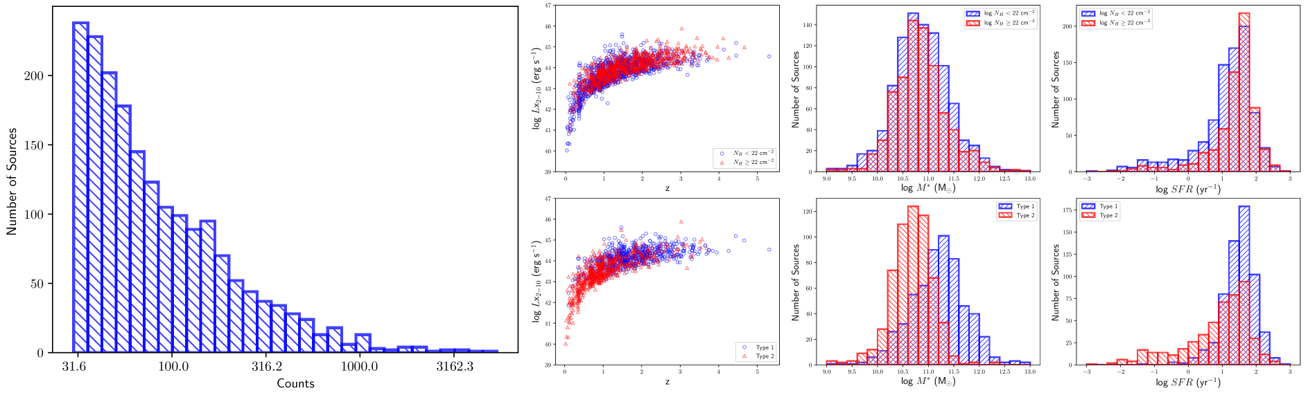
Figure 1: Chandra COSMOS-Legacy survey selected sample properties: (top, left) distribution of source $0.5-7$ keV net counts. The remaining plots (columns from left to right) depict survey properties including: X-ray luminosity vs redshift, stellar mass, and star formation rate. These are then colored according to (top row) obscuring column density, and (bottom row) optically classified AGN type.

The 4.6Ms CCLS covers the 2 deg² COSMOS field to a depth of $2\times 10^{-16}$ erg cm^-2 s^-1 in $0.5-2.0$ keV. The full catalog contains 4016 sources, with a full multiwavelength characterization and both photometric and spectroscopic redshifts available (Marchesi et al. 2016a) and also stellar mass and SFR computed with spectral energy distribution fitting (Suh et al. 2019, 2020). Moreover, X-ray spectral analysis results are available for $\sim$1900 sources with more than 30 counts in the $0.5-7$ keV (Marchesi et al. 2016b). We adopt the best-fit X-ray spectral models from this last catalog in our analysis, as described in Section 3.

2.1 Source Selection

From the full CCLS, we select sources with a minimum of 30 counts in $0.5-7.0$ keV, as in Marchesi et al. (2016b), where good fits to the continuum are available, to define our primary sample of $\sim 1900$ sources. The multiwavelength identifications made for the CCLS sources provide additional information permitting further division of the sample by redshift, as well as environmental properties (e.g., luminosity, obscuration, star formation rate). Distributions of these properties for the selected sample may be found in Figure 1, including $0.5-7.0$ keV net counts.

3 Stacking

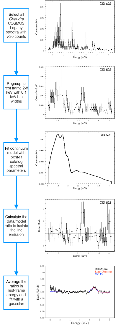
Figure 2: Schematic of the selected stacking method from reprocessed Chandra spectra through Fe K$\alpha$ line emission Gaussian fits. The first four panels depict the stacking process for an example source, CID 522, while the last panel shows the averaged data/model ratio for all of the sources.

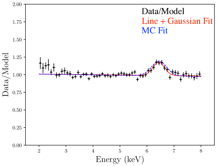
Figure 3: Average data/model ratio for the CCLS sources (black data points). This ratio is fit with a line + Gaussian model (red) to investigate the average properties of the Fe K$\alpha$ emission line at 6.4 keV. The model then undergoes a Monte Carlo analysis to determine the best-fit parameters (blue).

Our stacking analysis closely follows the methodology of Chaudhary et al. 2012 (see also Brusa et al. 2005; Corral et al. 2008, 2011; Walton et al. 2015). A schematic example of this method is shown in Figure 2. We primarily make use of CIAO 4.12, CALDB 4.8.2, and Sherpa, unless otherwise noted.

For each source, we isolate an energy band corresponding to the Chandra hard X-ray band, $2-8$ keV rest frame ($\frac{2.0}{1+z}-\frac{8.0}{1+z}$ keV), preferentially using spectroscopic redshifts, if available. The sources are regrouped using grppha in the HEASARC FTOOLS sub-package such that each channel is limited to this calculated waveband and rebinned in bin widths of 100 eV in rest frame ($\frac{0.1}{1+z}$ keV). With bin widths of 100 eV we capture important details of the spectra, especially surrounding the Fe K$\alpha$ emission line, while still maintaining significant counts within each energy bin, due to the spectral resolution of Chandra.

The model continuum is defined based on the spectral analysis of the CCLS from Marchesi et al. (2016b). Our spectral fits use Cstat statistics (based on Cash statistics; Cash 1979) and proper modeling of the Chandra background (Marchesi et al. 2016b). Galactic absorption is fixed to the average column density observed in the direction of the COSMOS field ($\text{N}_{H}=2.6\times 10^{20}$ cm^-2; Kalberla et al. 2005).

The source spectral models vary and are informed by the Marchesi et al. (2016b) best fits. In Marchesi et al. (2016b), rather than assuming a single absorbed power law slope for every source, sources with $30<\text{counts}<70$ are fit with a fixed $\Gamma=1.9$, while in sources with higher counts the power law slopes are left free to vary. We adopt the best fit $\Gamma$ from this analysis for both of these count regimes. The photoelectric absorption intrinsic to the AGN is fixed directly from the best-fit column densities. An unabsorbed second power law component ($\Gamma_{1}=\Gamma_{2}$) is required for some sources in Marchesi et al. (2016b) and has been included in our continuum fits for these individual sources. In some cases, the best-fit model parameters observed in Marchesi et al. (2016b) are unphysical due to limited count statistics (e.g., $\Gamma$ is very flat). However, since we are only interested in an accurate phenomenological characterization of the continuum, unphysical continuum models do not adversely impact our analysis.

After fitting the continuum, we calculate the ratio of the data to our best-fit continuum model. Since our analysis first regroups each source into the same number of bins of equal width (100 eV rest frame) from the $2-8$ keV rest frame, the bins of each source spectra line up exactly in rest frame, which means that we can directly add and average all of the sources without further modifying the data/model ratios. We stack each source and calculate the average ratio for each bin in energy. This yields an average data/model ratio for the selected $\sim 2000$ sources in the CCLS (Figure 3).

Since the focus of our analysis is on the Fe K$\alpha$ emission, our methodology deviates from that of Chaudhary et al. (2012). Rather than multiplying our data/model ratios by a single assumed power law (E^-Γ) to convert it back to an averaged spectrum, we instead continue our analysis by fitting emission lines to the data/model ratio. We tested the accuracy of extracting the Gaussian widths using this more simplistic method on simulated data/model ratios, and find that while both methods are able to consistently recover the simulated Gaussian and equivalent widths to better than $0.1\%$ of the input width ($\sigma=0.1,0.25,0.35,0.5$), fitting the data/model ratio is typically more precise by 6 decimal places.

The CCLS field is rich in multiwavelength data which uniquely allows us to break down the average data/model ratio as a function of observables, including: redshift, luminosity, star formation rate ($SFR$), stellar mass ($M^{*}$), optically-informed AGN type, obscuring column density ($N_{H}$), and observed $0.5-7.0$ keV spectral counts. Binning our sample by the total source spectral counts acts as a test to assess whether or not we are biasing our results with the highest S/N sources. Bins of AGN Type are separated into the Type 1/Type 2 designations as informed by their optical counterpart matches (see Marchesi et al. 2016a for a description of the multiwavelength CCLS catalog match). Similarly, $N_{H}$ is separated into bins of unobscured ($\log N_{H}<20$ cm^-2; $20<\log N_{H}<22$ cm^-2) and obscured ($\log N_{H}>22$ cm^-2). While a majority of the “unobscured” sources are real unobscured sources, there may exist a population of heavily obscured sources ($\log N_{H}>23$ cm^-2) hiding within this subsample for which the standard spectral fitting in Marchesi et al. (2016b) did not work properly. These candidate CT AGN are further analyzed in Lanzuisi et al. (2018).

For the remaining properties, we use dynamically sized bins where the bin size is determined by adding sources to achieve a minimum total number of counts ($0.5-7.0$ keV) in each bin. For this analysis, we use a minimum count threshold of $\sim 40,000$ total counts. In this way, we are using the $0.5-7.0$ keV total counts as a proxy for achieving a high S/N in the average data/model ratio bins. We include the full, broad range of observed properties in the analysis, but note that only 21 sources fall below $\log M^{*}<9$, while only 7 sources fall above $z>4$.

4 Iron K$\alpha$ Line Fitting

4.1 Gaussian Line Fits

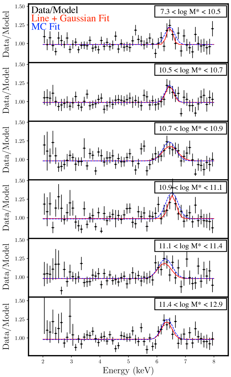
Figure 4: Data/Model ratio broken into bins of stellar mass (black) with the best line+Gaussian (red), and MC (blue) fits.

Figure 5: Data/Model ratio broken into bins of column density (black) with the best line+Gaussian (red), and MC (blue) fits.

By design we have removed the continuum in each spectrum by calculating the data/model ratio. Thus, for each source, the excess above unity consists of isolated X-ray emission lines that likely originate near the black hole. From these stacked average data/model ratios, we fit the excess above the continuum at 6.4 keV with a Gaussian Fe K$\alpha$ emission line model.

The fits are made using curve_fit, part of the optimize module in the python scipy library. We assume that we have correctly redshifted all sources such that our data/model ratios are at rest frame ($z=0$) and the Fe K$\alpha$ emission line is represented by a Gaussian frozen at 6.4 keV. The function we use is an additive model of a straight line continuum (representing where the model exactly fits the data, i.e., unity) and Gaussian shape: $ratio=(m\times E+b)+C\times\exp(-(E-6.4)^{2}/2\sigma_{g}^{2})$, where $m$ is the line slope, $b$ is the line normalization, $C$ is the Gaussian amplitude, and $\sigma_{g}$ is the Gaussian width. Our initial conditions and [boundary conditions] are: $m=0$ $[-0.1\,,\,0.1]$, $b=1.0$ $[0.9\,,\,1.1]$, $C=1.0$ $[0.0\,,\,2.0]$, and $\sigma_{g}=0.1$ $[0.1\,,\,0.5]$. We used a Monte Carlo method to randomly resample the data/model ratios ($N=100$) and determine the best fit. We fit the line+Gaussian shape for the average stacked spectrum (Figure 3), as well as for each binned parameter (e.g., $M^{*}$, Figure 4; $N_{H}$, Figure 5; Additional parameter fits included in Appendix A).

To test our assumption that the average Fe K$\alpha$ emission line is centered at 6.4 keV and therefore not significantly impacted by e.g., different ionization states, or residual redshift effects, we allowed the centroid of the Gaussian line to vary, finding a best-fit centroid line energy of $6.45$ keV. We find that our results are not significantly impacted by setting the Gaussian line energy as a free parameter (to within a few percent), and have thus adopted a fixed line energy for simplicity and to limit possible degeneracies in the fit (Table 1). We also test the impact of using photometric redshifts to fit the CCLS sample, when spec-z are not available, as is the case for $\sim$31% of the selected sample. We find the Gaussian widths fit using only sources with spec-z are within the errors of the full sample.

4.2 Relativistic Line Fits

The Gaussian fit is more simplistic than the relativistic line models that are typically used to measure $a$, the spin measurement parameter ($a=cJ/GM^{2}$, where M is the black hole mass, J is the angular momentum; $-1<a<1$) for sources with hundreds of thousands of counts. It is important to note that while we cannot duplicate the detail of an in-depth spin analysis of an individual, bright AGN using a stacking method that itself may smooth over interesting physics and could introduce systematic errors, our intent is to determine the “average” black hole spin and compare this spin with e.g., redshift, and other environmental variables. While we must make some assumptions to test these more complex relativistic fits (e.g., frozen model parameters), what we gain are new insights into the evolution of SMBHs and their host galaxies that are currently limited by observational constraints.

4.2.1 diskline

Figure 6: Average data/model ratio for the CCLS sources (black data points). This ratio is fit with a line + diskline model (red) with black hole spin parameter fixed at $a=0$.

We attempt to constrain the black hole spin parameter starting with the simplest of these relativistic line models, diskline, representing broadened line emission from the inner accretion disk with a non-spinning black hole ($a=0$; Fabian et al. 1989). We first freeze all parameters, except the normalization, at their default values (including LineE = 6.4 keV). We then systematically thaw these model parameters and fit the data using the Nelder-Mead Simplex optimization method; we test the goodness of fit with $\chi^{2}$ minimization (details of these fits are included in Appendix A.2). Ultimately we find a very good fit ($r\chi^{2}=0.413$) using this relativistic line model that assumes no black hole spin (Figure 6).

4.2.2 relline

Figure 7: Average data/model ratio for the CCLS sources (black data points). This ratio is fit with a line + relline model (red) with the black hole spin parameter, normalization, and inclination left to vary.

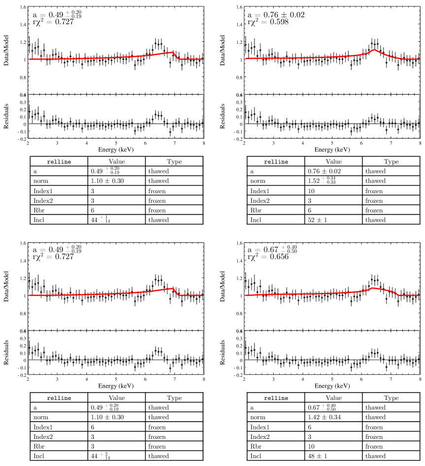
Figure 20: relline model fits to the average data/model ratio for all CCLS sources. The line energy is fixed at 6.4 keV while all other fixed parameters are frozen at default values, unless otherwise indicated. The relline spin parameter (a), the normalization, and the inclination are left free to vary. We explore the parameter space of the emissivity index for r $<$ Rbr (Index1) and the radius of emissivity change (Rbr) both above and below their typical values of 6: (top, left) Index1 $=3$; (top, right) Index1 $=10$; (bottom, left) Rbr $=3$; (bottom, right) Rbr = 10.

We find that while diskline provides a good fit to the average data/model ratio, it is not a fully relativistic model and does not adequately parameterize light bending. Thus, rather than assuming a static value for the black hole spin, we instead incorporate a more physical relativistic line model, relline, from relxill v1.3.3 (Dauser et al. 2010, 2013, 2014) to fit the black hole spin parameter, $a$. As with diskline, we start with the fewest thawed parameters before increasing the fit complexity by introducing additional free parameters. For all fits, we keep $a$ and the normalization of this relativistic line free. The other parameters of interest are kept static, including Index1$=$6, Index2$=$3, and Rbr$=$6, where the emissivity for the corona is defined as Index1, and Index2, for the regions Rin to Rbr, and Rbr to Rout, respectively. We first investigate how the inclination of the accretion disk impacts the shape of the relativistic line (Appendix, Figure 19) for inclination values of 45, 30, and 60 degrees, before testing the parameter space surrounding Index1 and Rbr (Appendix, Figure 20). The best-fit relativistic line model left inclination free to vary and set Index1$=10$, and found $a=0.76\pm 0.02$ ($r\chi^{2}=0.598$). The Fe K$\alpha$ emission line is not completely fit in this model, as shown in Figure 7, however, and a more complex model may be needed.

4.2.3 relline + Gaussian

Figure 8: Average data/model ratio for the CCLS sources (black data points). This ratio is fit with a line + relline + Gaussian model (red) with the black hole spin parameter, normalization, line energy, and inclination left to vary. The Gaussian width and normalization are also left free to vary in this best-fit model.

Since the single relline model left residuals around the Fe K$\alpha$ 6.4 keV emission line, we added a narrow Gaussian at 6.4 keV to the model to represent the combination of relativistically broadened and narrow Fe emission (a typical feature observed in AGN; Yaqoob & Padmanabhan 2004). A two component (broad + narrow) model fit to the Fe K$\alpha$ emission is also consistent with the best-fit model found for the stacked AGN in the 2XMM catalog (Chaudhary et al. 2012), and for the stacked 263 XMM-selected unabsorbed AGN spectra from the Vèron-Cetty and Vèron catalogs (Falocco et al. 2014).

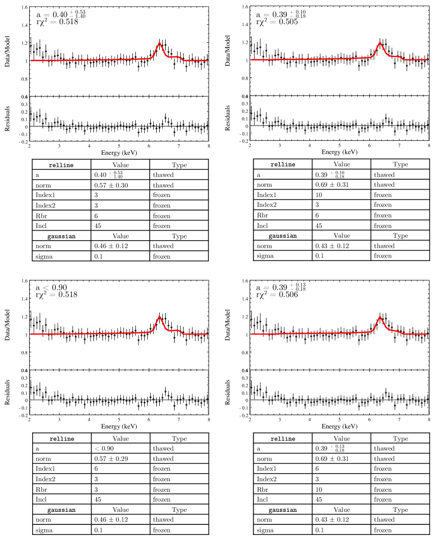
Figure 22: relline+gaussian model fits to the average data/model ratio for all CCLS sources. The relline and gaussian line energy are fixed at 6.4 keV, and the gaussian width is fixed to 0.1 keV (the size of our bins). All other fixed parameters are frozen at default values, unless otherwise indicated. The relline spin parameter (a) and normalization are left free to vary. We explore the parameter space of the emissivity index for r ¡ Rbr (Index1) and the radius of emissivity change (Rbr) both above and below their typical values of 6: (top, left) Index1 $=3$; (top, right) Index $1=10$; (bottom, left) Rbr $=3$; (bottom, right) Rbr $=10$.

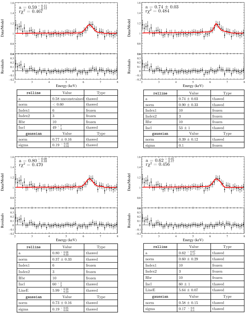
Figure 23: relline+gaussian model fits to the average data/model ratio for all CCLS sources. The gaussian line energy is fixed at 6.4 keV. All other fixed parameters are frozen at default values, unless otherwise indicated. The relline spin parameter (a), inclination, and both relline and gaussian normalizations are left free to vary. Building on previous fit results, we further explore the parameter space: (top, left) Index1 $=6$, Rbr $=10$, gaussian sigma left free to vary; (top, right) Index1 $=10$, Rbr $=10$; (bottom, left) Index1 $=6$, Rbr $=10$, gaussian sigma left free to vary, relline line energy left free to vary; (bottom, right) Index1 $=10$, Rbr $=10$, gaussian sigma left free to vary, relline line energy left free to vary.

Similar to the process for the single relline model, we systematically stepped through the parameter space, starting with inclination of the relline accretion disk (Appendix, Figure 21). The additional Gaussian width was frozen at 0.1 keV, while the normalization was left free. We then tested the parameter space surrounding Index1 and Rbr (Appendix, Figure 22), and similarly found a better fit when Index1$=10$. Finally, we varied the width of the additional Gaussian in addition to the relline parameters (Appendix, Figure 23). The best-fit relativistic line + Gaussian model set the relline inclination and line energy, and the Gaussian width free to vary (Figure 12), although many of the model combinations we tried yielded very good fits. In this model, Index1$=10$, Index2$=3$, and Rbr$=10$, and the black hole spin parameter was found to be $a=0.62~{}\begin{subarray}{c}+0.07\\ -0.17\end{subarray}$ ($r\chi^{2}=0.456$).

5 Discussion

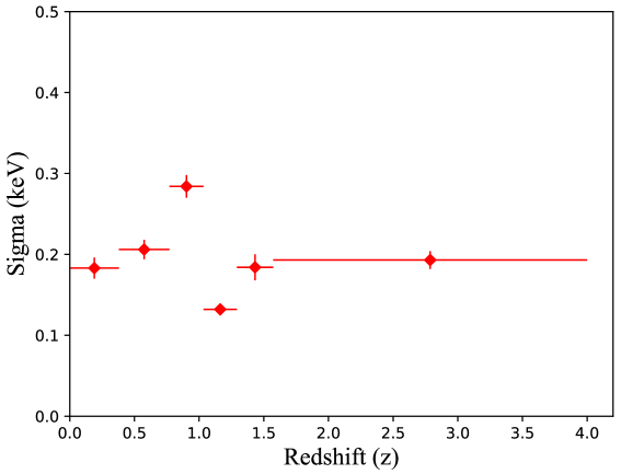
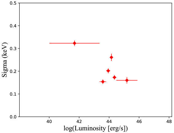
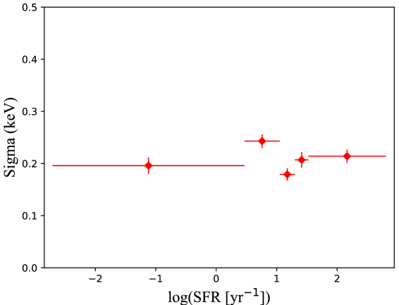
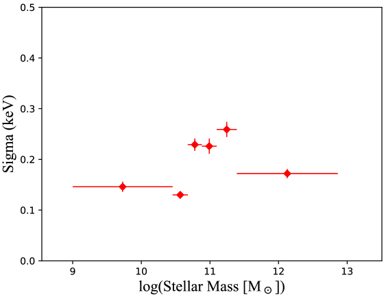
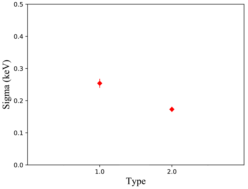
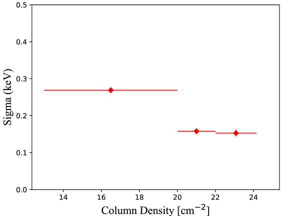
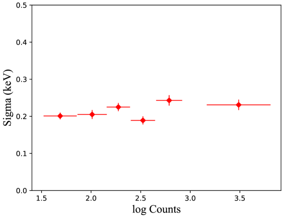
Figure 9: Evolution of the best-fit Gaussian widths in bins of observational properties.

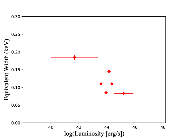
Figure 10: Evolution of the equivalent widths calculated from the best-fit Gaussian models for the CCLS sample in bins of $2-10$ keV X-ray luminosity.

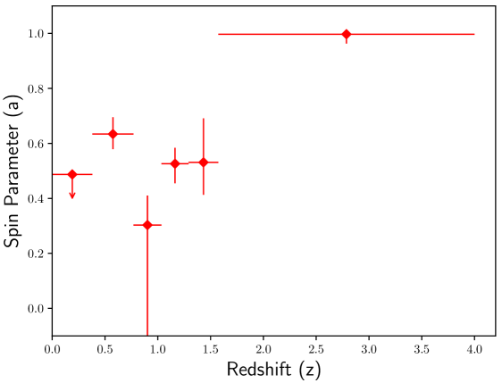
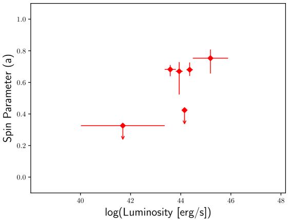
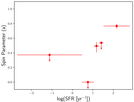
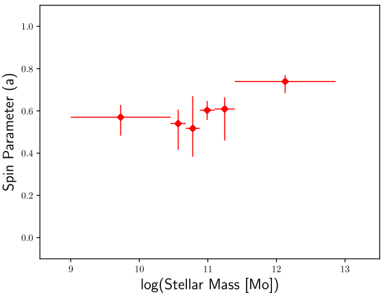
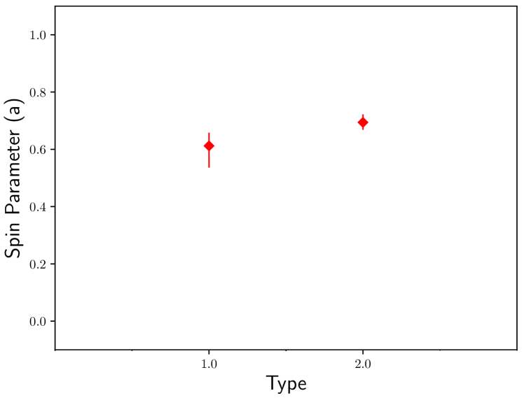
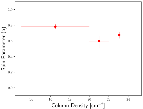
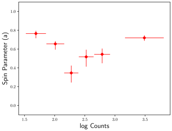
Figure 11: Evolution of the best-fit relline spin parameter a in bins of observational properties. Arrows indicate where the spin parameter represents an upper limit and is not well constrained.

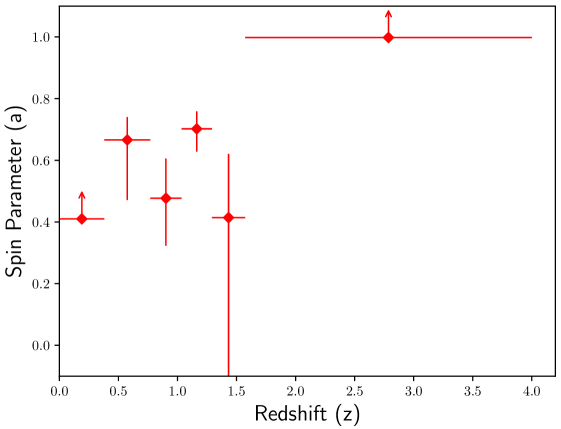
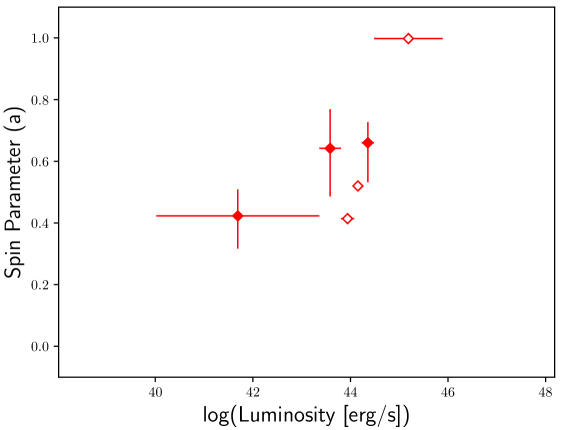
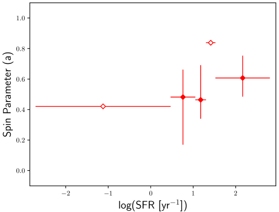
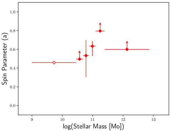
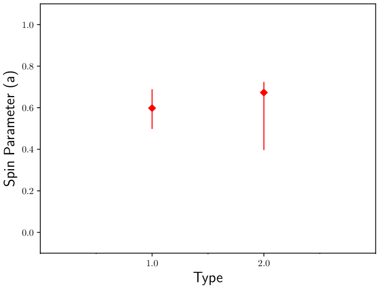
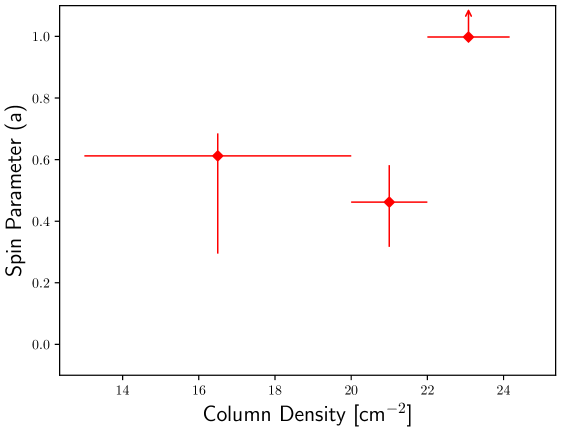
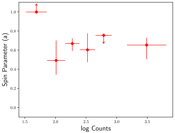
Figure 12: Evolution of the best-fit relline+Gaussian spin parameter a in bins of observational properties. Arrows indicate where the spin parameter represents an upper limit and is not well constrained. Empty markers indicate an unconstrained spin parameter.

Table 1: Best-fit Gaussian widths, relline and relline+Gaussian black hole spin measurements for the full average CCLS sample. Also included are the best-fit parameters for the CCLS sample further divided by observational properties. $U$ indicates an unconstrained parameter.

		Gaussian		relline	relline+Gaussian
		$\sigma$	EW	a	a
	All Sources	$0.28\pm 0.05$	$0.13\pm 0.02$	$0.76\pm 0.02$	$0.62~{}\begin{subarray}{c}+0.07\\ -0.17\end{subarray}$
	Bins	$\sigma$	EW	a
$z$	[0.00, 0.38]	$0.18\pm 0.01$	$0.20\pm 0.01$	$<0.49$	$>0.41$
	[0.38, 0.77]	$0.21\pm 0.01$	$0.12\pm 0.01$	$0.63\pm 0.06$	$0.67~{}\begin{subarray}{c}+0.07\\ -0.20\end{subarray}$
	[0.77, 1.03]	$0.28\pm 0.01$	$0.15\pm 0.01$	$0.30~{}\begin{subarray}{c}+0.11\\ -0.71\end{subarray}$	$0.48~{}\begin{subarray}{c}+0.13\\ -0.15\end{subarray}$
	[1.03, 1.29]	$0.13\pm 0.01$	$0.12\pm 0.003$	$0.53~{}\begin{subarray}{c}+0.06\\ -0.07\end{subarray}$	$0.70~{}\begin{subarray}{c}+0.06\\ -0.07\end{subarray}$
	[1.29, 1.57]	$0.18\pm 0.02$	$0.07\pm 0.005$	$0.53~{}\begin{subarray}{c}+0.16\\ -0.12\end{subarray}$	$0.41~{}\begin{subarray}{c}+0.21\\ -1.03\end{subarray}$
	[1.57, 4.00]	$0.19\pm 0.01$	$0.09\pm 0.004$	$0.99~{}\begin{subarray}{c}+0.001\\ -0.03\end{subarray}$	$>0.99$
log $L_{x}$	[40.0, 43.4]	$0.32\pm 0.01$	$0.18\pm 0.01$	$<0.33$	$0.42~{}\begin{subarray}{c}+0.09\\ -0.11\end{subarray}$
	[43.4, 43.8]	$0.15\pm 0.01$	$0.11\pm 0.004$	$0.68~{}\begin{subarray}{c}+0.03\\ -0.04\end{subarray}$	$0.64~{}\begin{subarray}{c}+0.13\\ -0.16\end{subarray}$
	[43.8, 44.1]	$0.20\pm 0.01$	$0.09\pm 0.004$	$0.67~{}\begin{subarray}{c}+0.06\\ -0.15\end{subarray}$	$0.41~{}U$
	[44.1, 44.2]	$0.26\pm 0.02$	$0.15\pm 0.01$	$<0.42$	$0.52~{}U$
	[44.2, 44.5]	$0.17\pm 0.01$	$0.11\pm 0.004$	$0.68~{}\begin{subarray}{c}+0.05\\ -0.04\end{subarray}$	$0.66~{}\begin{subarray}{c}+0.07\\ -0.13\end{subarray}$
	[44.5, 45.9]	$0.16\pm 0.01$	$0.08\pm 0.01$	$0.75~{}\begin{subarray}{c}+0.06\\ -0.10\end{subarray}$	$0.99~{}U$
log $SFR$	[-2.71, 0.47]	$0.20\pm 0.02$	$0.11\pm 0.01$	$<0.37$	$0.42~{}U$
	[0.47, 1.05]	$0.24\pm 0.01$	$0.12\pm 0.01$	$<0.00$	$0.48~{}\begin{subarray}{c}+0.18\\ -0.31\end{subarray}$
	[1.05, 1.30]	$0.18\pm 0.01$	$0.15\pm 0.01$	$0.49~{}\begin{subarray}{c}+0.05\\ -0.09\end{subarray}$	$0.46~{}\begin{subarray}{c}+0.23\\ -0.12\end{subarray}$
	[1.30, 1.52]	$0.21\pm 0.02$	$0.08\pm 0.01$	$<0.54$	$0.84~{}U$
	[1.52, 2.80]	$0.21\pm 0.01$	$0.11\pm 0.004$	$0.77~{}\begin{subarray}{c}+0.03\\ -0.04\end{subarray}$	$0.61~{}\begin{subarray}{c}+0.15\\ -0.12\end{subarray}$
log $M^{*}$	[9.0, 10.5]	$0.15\pm 0.01$	$0.08\pm 0.003$	$0.57~{}\begin{subarray}{c}+0.06\\ -0.09\end{subarray}$	$0.46~{}U$
	[10.5, 10.7]	$0.13\pm 0.004$	$0.08\pm 0.003$	$0.54~{}\begin{subarray}{c}+0.12\\ -0.09\end{subarray}$	$>0.50$
	[10.7, 10.9]	$0.23\pm 0.01$	$0.13\pm 0.01$	$0.52~{}\begin{subarray}{c}+0.15\\ -0.13\end{subarray}$	$0.53~{}\begin{subarray}{c}+0.16\\ -0.23\end{subarray}$
	[10.9, 11.1]	$0.23\pm 0.02$	$0.14\pm 0.01$	$0.60~{}\begin{subarray}{c}+0.04\\ -0.05\end{subarray}$	$0.63~{}\begin{subarray}{c}+0.06\\ -0.11\end{subarray}$
	[11.1, 11.4]	$0.26\pm 0.02$	$0.13\pm 0.01$	$0.61~{}\begin{subarray}{c}+0.06\\ -0.15\end{subarray}$	$>0.80$
	[11.4, 12.9]	$0.17\pm 0.01$	$0.12\pm 0.01$	$0.74~{}\begin{subarray}{c}+0.03\\ -0.06\end{subarray}$	$>0.60$
Type	1	$0.25\pm 0.01$	$0.11\pm 0.005$	$0.61~{}\begin{subarray}{c}+0.05\\ -0.08\end{subarray}$	$0.60~{}\begin{subarray}{c}+0.09\\ -0.10\end{subarray}$
	2	$0.17\pm 0.01$	$0.10\pm 0.003$	$0.69\pm 0.03$	$0.67~{}\begin{subarray}{c}+0.05\\ -0.28\end{subarray}$
log $N_{H}$	[13.0, 20.0]	$0.27\pm 0.01$	$0.14\pm 0.004$	$0.78\pm 0.03$	$0.61~{}\begin{subarray}{c}+0.07\\ -0.32\end{subarray}$
	[20.0, 22.0]	$0.16\pm 0.01$	$0.09\pm 0.003$	$0.60~{}\begin{subarray}{c}+0.06\\ -0.09\end{subarray}$	$0.46~{}\begin{subarray}{c}+0.12\\ -0.15\end{subarray}$
	[22.0, 24.2]	$0.15\pm 0.01$	$0.07\pm 0.003$	$0.67\pm 0.04$	$0.99~{}\begin{subarray}{c}+0.0003\\ -0.004\end{subarray}$
Counts	[30, 68]	$0.20\pm 0.01$	$0.09\pm 0.004$	$0.77~{}\begin{subarray}{c}+0.03\\ -0.05\end{subarray}$	$>0.99$
	[68, 137]	$0.21\pm 0.01$	$0.10\pm 0.004$	$0.66~{}\begin{subarray}{c}+0.03\\ -0.06\end{subarray}$	$0.49~{}\begin{subarray}{c}+0.21\\ -0.15\end{subarray}$
	[137, 239]	$0.23\pm 0.01$	$0.13\pm 0.01$	$0.35~{}\begin{subarray}{c}+0.08\\ -0.10\end{subarray}$	$0.67~{}\begin{subarray}{c}+0.06\\ -0.08\end{subarray}$
	[239, 427]	$0.19\pm 0.01$	$0.10\pm 0.004$	$0.52~{}\begin{subarray}{c}+0.08\\ -0.10\end{subarray}$	$0.60~{}\begin{subarray}{c}+0.17\\ -0.13\end{subarray}$
	[427, 798]	$0.24\pm 0.01$	$0.11\pm 0.004$	$0.54~{}\begin{subarray}{c}+0.06\\ -0.10\end{subarray}$	$<0.75$
	[798, 5355]	$0.23\pm 0.01$	$0.15\pm 0.01$	$0.72\pm 0.03$	$0.65~{}\begin{subarray}{c}+0.08\\ -0.15\end{subarray}$

Table 2: Slope of a linear fit to the Gaussian width, relline and relline+Gaussian black hole spin parameters as a function of observational properties. The statistical significance of these slopes are given by the column $\sigma$.

	Gaussian		relline		relline+Gaussian
Parameter	Slope	($\sigma$)	Slope	($\sigma$)	Slope	($\sigma$)
$z$	$-0.001\pm 0.034$	$0.03$	$0.195\pm 0.083$	$2.3$	$0.190\pm 0.083$	2.3
log $L_{x}$	$-0.046\pm 0.019$	$2.4$	$0.111\pm 0.047$	$2.4$	$0.130\pm 0.066$	2.0
log $SFR$	$0.002\pm 0.013$	$0.2$	$0.112\pm 0.115$	$1.0$	$0.077\pm 0.066$	1.2
log $M^{*}$	$0.026\pm 0.029$	$0.9$	$0.076\pm 0.032$	$2.4$	$0.089\pm 0.062$	1.4
log $N_{H}$	$-0.019\pm 0.005$	$3.8$	$-0.020\pm 0.018$	$1.1$	$0.044\pm 0.070$	0.6
Counts	$0.017\pm 0.013$	$1.3$	$-0.003\pm 0.122$	$0.02$	$-0.084\pm 0.129$	0.7

5.1 The Average CCLS Spin

By stacking the CCLS sources, we are able to extract the average Fe K$\alpha$ emission line profile at 6.4 keV. We first fit this emission line with a Gaussian model and find a broadened line profile with a Gaussian width of $\sigma_{g}=0.28\pm 0.05$ and equivalent width of $\text{EW}=0.13\pm 0.02$ (Table 1). In a similar study with XMM, Corral et al. (2008) and Corral et al. (2011) do not find compelling evidence for broad relativistic Fe K$\alpha$ emission. They do, however, place upper limits on the equivalent width of a relativistic line at $\text{EW}=0.40$ keV and $\text{EW}=0.23$ keV, respectively. Other stacking analyses with XMM survey fields likewise do not find evidence for relativistically broadened Fe K$\alpha$ line emission (e.g., Corral et al. 2008; Iwasawa et al. 2012; Falocco et al. 2013; Liu et al. 2016).

The width of the Fe K$\alpha$ emission line that we find suggests that the average spectra in the CCLS sample is undergoing mild relativistic broadening. This broadening, however, may be explained by a variety of processes other than a relativistically spinning black hole, including disk inclination, reflection from circumnuclear clouds, and physical processes like gas turbulence and ionization.

To help constrain the origin of this broad Fe K$\alpha$ emission line profile, we then fit the averaged CCLS spectra with relativistic emission line models. Starting with diskline, a broadened emission line for a non-spinning black hole, and working up to the relativistic line model relline for which the black hole spin parameter, $a$, may be constrained. We find the single best-fit relline model yields a spin measurement of $0.76\pm 0.02$, while the more complex, best-fit relline + Gaussian model finds $a=0.62~{}\begin{subarray}{c}+0.07\\ -0.17\end{subarray}$. These are comparable to the average prograde spin, $\text{a}\sim 0.7$, found by Walton et al. (2015) for 27 lensed quasars.

The average spin we find for both relativistic models suggests that the dominant growth mechanism for this AGN population is likely merger dominated. Relativistic numerical simulations from Berti & Volonteri (2008) show that the average black hole spin from randomly oriented, isotropically distributed major mergers is $a\sim 0.69$, which falls between our two best-fit spins. Chaotic accretion episodes cause the spin to slow, while prolonged accretion aligned with the spin direction can spin up the black hole. Thus, while major mergers likely dominate our population, there may be contributions from prograde accretion (relline model) and/or chaotic accretion (relline + Gaussian model).

5.2 Black Hole Spin: Evolution and Environment

We take this analysis a step further by separating our average data/model ratios in bins of observed properties to investigate whether evolution and environment may be linked to the Fe K$\alpha$ emission line profile, and by extension, the spin of the SMBH (Figures 9, 11; Tables 1, 2). The relativistic line models used in the following analysis are based on the best-fit parameters for the single relline model, and the more complex relline + Gaussian models. In order to constrain the spin parameter in the complex model for these smaller bins, however, all parameters, excluding the normalization and spin, had to be frozen to their best-fit values. We fit a line to our observed parameter bins using a non-linear least-squares optimization with scipy curve_fit to provide a rough estimate of the strength of any possible parameter evolution.

5.2.1 Evolution to $z\sim 5.3$

Binning by redshift, we find no evidence for evolution of the Gaussian width (Figure 9; top, left), best fit with a slope of $m_{z}=-0.001\pm 0.034$ (slope significance; $\sigma=0.03$). The black hole spin parameters extracted have a stronger slope than the Gaussian widths for both the single relativistic line and the more complex relline + Gaussian model (Table 2), and these slopes are consistent (relline: $m_{z}=0.195\pm 0.083$, $\sigma=2.3$; relline+Gaussian: $m_{z}=0.190\pm 0.083$, $\sigma=2.3$). However, this fit is heavily influenced by the highest redshift bin where sources are fainter and less abundant. Excluding this high-z bin, the spin parameter does not appear to evolve with redshift.

5.2.2 Luminosity

Interestingly, we find anti-correlated dependencies of the Gaussian width and black hole spin parameter in bins of $2-10$ keV luminosity (Figure 9, 11; top, right). The Gaussian widths evolve according to a best-fit slope of $m_{Lx}=-0.046\pm 0.019$ ($\sigma=2.4$). The black hole spin best-fit slopes in comparison are $m_{Lx}=0.111\pm 0.047$ ($\sigma=2.4$), and $m_{Lx}=0.130\pm 0.066$ ($\sigma=2.0$) for the single relline and relline + Gaussian models, respectively. These fits, however, are predominately influenced by the lowest luminosity bin. Furthermore, 50% of the extracted spins are unconstrained for the more complex relativistic model. Perhaps unsurprisingly, the Gaussian widths (and equivalent widths; Figure 10) exhibit an inverse relationship that is consistent with the X-ray Baldwin effect (the inverse correlation between the equivalent width and $L_{X}$; Iwasawa & Taniguchi 1993). The black hole spin parameters, however, increase with increasing luminosity. This may reflect the interesting impact that spin has on the AGN Eddington limit. For faster spinning black holes, the ISCO moves inward toward the event horizon, enabling stable orbits deeper within the gravitational potential well, and thus enabling more energy to be extracted from inflating material, increasing the AGN’s capacity to be more luminous.

5.2.3 Stellar Mass and SFR

From observational evidence, it has become increasingly clear that there exists a correlation between the growth of the SMBH and its host galaxy (Ferrarese & Merritt 2000), however, there is disagreement about which galaxy property ($SFR$ or $M^{*}$) is most fundamentally linked with AGN activity (e.g., Chen et al. 2013; Yang et al. 2018, 2019; Suh et al. 2019; Stemo et al. 2020). By binning the CCLS sample by $SFR$ and $M^{*}$, we may test the connection between these galaxy properties and the shape of the Fe K$\alpha$ line profile, and by extension, the AGN activity (Figure 9, 11; second row, left and right, respectively).

For our Gaussian fits, we find no evidence linking an evolution of $SFR$ with broadened Fe K$\alpha$ ($m_{SFR}=0.002\pm 0.013$; $\sigma=0.2$), while there does exist slightly more compelling evidence for a connection between $M^{*}$ and broadened Fe K$\alpha$ ($m_{M^{*}}=0.026\pm 0.029$; $\sigma=0.9$), albeit not statistically significant. This does appear to be strongly influenced by the most massive bin, where fewer high mass sources may unduly skew the result.

The relline best-fit spin parameters exhibit stronger positive slopes for both $SFR$ ($m_{SFR}=0.112\pm 0.115$; $\sigma=1.0$) and $M^{*}$ ($m_{SFR}=0.076\pm 0.032$; $\sigma=2.4$) compared to the Gaussian evolution, however, the spin parameters in the $SFR$ bins are not well constrained: $60\%$ are upper limits. The relline + Gaussian best-fit spin parameter slopes for $SFR$ and $M^{*}$ are more consistent than the single relline model with $m_{SFR}=0.077\pm 0.066$ ($\sigma=1.2$), and $m_{SFR}=0.089\pm 0.062$ ($\sigma=1.4$), respectively. The relationship between $M^{*}$ and black hole spin is not quite significant for the single relline model, but could point to stellar mass being the predominate driver of the observed connection between the growth of the black hole and its host galaxy.

Neither of the relativistic models exhibit an anti-correlation between the spin parameter and stellar mass, that (assuming stellar mass is a good proxy for black hole mass) is exhibited by the few dozen currently known black hole spins (See Reynolds 2019 Figure 3). While it is expected that the AGN population with known black hole spins suffers from selection biases and low number statistics that may unduly influence this observed relationship, Pacucci & Loeb (2020) theoretically predict a similar trend wherein the spin parameter decreases with increasing black hole mass. Thus, our conclusions must be treated cautiously.

5.2.4 Obscuration and AGN Type

We compare the evolution of the Gaussian width and black hole spin parameter with the optically defined AGN type (Figure 9, 11; third row, left), and obscuring column density (Figure 9, 11; third row, right), as they are both commonly used to select AGN as obscured or unobscured. There is some evidence that these two methods may be selecting slightly different AGN populations (e.g., Merloni et al. 2014), however, Civano et al. (2016) compared the selection of AGN by obscuration and Type in Chandra-COSMOS, and found a good match between the two methods (see also Marchesi et al. 2016b for CCLS).

The Gaussian widths of the “unobscured” sources broaden as they become more “obscured” for both AGN type and obscuring column density, and the width values are consistent across both properties. This inverse relationship for column density is best-fit with a slope of $m_{NH}=-0.019\pm 0.005$ ($\sigma=3.8$).

There appears to be a comparable trend for column density with black hole spin parameter, albeit less significant ($m_{NH}=-0.020\pm 0.018$; $\sigma=1.1$) for the single relline model. The highest column density bin in the relline + Gaussian model is not well constrained and significantly impacts the slope calculated for these best-fit parameters. Without this bin, the relationship between spin and column density would be more consistent with that of the single relativistic line model. AGN type for both relativistic models, however, does not exhibit this inverse relationship with black hole spin, although the slope of the relline + Gaussian model is less significant than the single model.

It is possible that the inverse relationship with column density exhibited by both the Gaussian and relativistic models is influenced by a potentially large number of hidden, obscured sources where the Marchesi et al. (2016b) spectral fits failed to properly measure $\Gamma$ and $N_{H}$. Observational evidence for this comes from measurements of the line EW, in which large Fe K$\alpha$ EW are an indicator of large, even CT, obscuration. The EW of our $\log N_{H}<20$ cm^-2 bin is significantly higher than the column density bins with higher obscuration (Table 1).

5.2.5 Total $0.5-7.0$ keV Counts

We break down our data/model ratios as a function of source $0.5-7$ keV total counts to test that we are not biasing our results with the highest count sources (Figure 9, 11; bottom).

We first fit the Gaussian width as a function of counts and find a slope of $m_{cts}=0.017\pm 0.013$ ($\sigma=1.3$). The flatness of this slope suggests that the S/N from a single source does not unduly influence the results of our stacking method. Similarly, we do not find evolution of the black hole spin parameter with counts for the single relline model ($m_{cts}=-0.003\pm 0.122$; $\sigma=0.02$). There is a stronger relationship for the slope of the best-fit relline + Gaussian model spin parameters ($m_{cts}=-0.084\pm 0.129$; $\sigma=0.02$), however, this is significantly influenced by a single bin at low counts where we expect the stacked data/model ratios to be considerably noisier.

6 Conclusions

The CCLS is a rich multiwavelength environment for probing the connection between the AGN and its host galaxy. In this work, we investigated the connection between observed properties and the profiles of the Fe K$\alpha$ line emission, with implications for the average spin of SMBH across cosmic time and AGN population.

We select all CCLS sources with $>30$ net counts in $0.5-7.0$ keV. For each of these sources we regroup the spectra from 2 to 8 keV in 100 eV bins (rest-frame). Using the best-fit spectral models from Marchesi et al. (2016b), we fit the continuum and calculate the data/model ratios to isolate the Fe K$\alpha$ emission line at 6.4 keV. These ratios are then averaged over the entire sample. We further divide the sample by observational properties and average these bins to test the influence of these properties on the Fe K$\alpha$ line profile.

1. We find the average CCLS spectrum has broad Fe K$\alpha$ line emission with Gaussian width $\sigma_{g}=0.28\pm 0.05$ and equivalent width $EW=0.13\pm 0.02$. The broad Fe K$\alpha$ line emission may also be fit with a broadened relativistic emission line with black hole spin parameter $a=0.76\pm 0.02$, or better fit with a more complex relline + Gaussian model with $a=0.62~{}\begin{subarray}{c}+0.07\\ -0.17\end{subarray}$. These black hole spin estimates are consistent with the results from Walton et al. (2015) for lensed quasars. The dominant growth mechanism for the CCLS population is likely major mergers, with perhaps a smaller contribution from chaotic accretion and/or prograde accretion events (Berti & Volonteri 2008).

2. When dividing our sample by observational properties, we find little evolution of the Gaussian line width or black hole spin with redshift (although this conclusion excludes the highest redshift bin). Furthermore, we find no correlation between these measurements with counts in $0.5-7.0$ keV. This demonstrates that the method we are using is not biased by the highest count sources.

3. We find an interesting trend with luminosity such that the black hole spin parameter increases with increasing luminosity, while the Gaussian width (and equivalent width) are inversely correlated with increasing luminosity, consistent with the X-ray Baldwin effect. The positive trend observed with spin parameter and luminosity may be an effect from the improved accretion stability afforded by a spinning black hole, increasing the capacity of sources to become more luminous.

4. We find a possible trend in the Fe K$\alpha$ line width with stellar mass, but less so for $SFR$. This may suggest that stellar mass is the fundamental property driving the observed link between black hole and galaxy growth. Black hole spin, however, exhibits a stronger trend in $SFR$ compared to $M^{*}$, but the spin parameters are not well constrained in this case. Assuming stellar mass is a good proxy for black hole mass, the relationship we find is opposite to what is observed (and theorized; Pacucci & Loeb 2020) for the few dozen nearby sources for which black hole spins have been measured (Reynolds 2019).

5. We find a connection between obscuration and the Fe K$\alpha$ line width and black hole spin parameter, which is consistent for both optically classified AGN types and obscuration based on X-ray spectral fits of obscuring column density. Unobscured sources (optical Type 1; $\log N_{H}<20$ cm^-2) have broader Fe K$\alpha$ emission line widths compared to the more obscured sources. Likewise, unobscured sources have higher black hole spins than obscured sources, although this trend is much less significant. This result may be influenced by a potentially significant, heavily obscured AGN population “hiding” amongst the unobscured sources.

This work demonstrates the advantages of using Chandra for AGN population studies. The availability of rich, deep multiwavlength fields and high spectral resolution allow for production of statistically significant samples that can be used to investigate otherwise challenging observed properties (e.g., black hole spin) and to uniquely probe the black hole-galaxy connection. As we look toward the future and plan the next generation of great observatories (e.g., eROSITA, Athena, STROBE-X, and Lynx), focusing on wide area, high spatial resolution instruments will be crucial to our understanding of the AGN population.

Appendix A Fe K$\alpha$ Line Fitting Continued

A.1 Gaussian Line

We have appended the data/model ratio Gaussian fits for each stacked bin for the host galaxy and black hole properties in our analysis: redshift (Figure 13), X-ray luminosity (Figure 14), star formation rate (Figure 15), AGN type (Figure 16), and Counts (Figure 17). For each data/model ratio, we adopt the Monte Carlo (N=100) best-fit parameters. These parameters are listed in Table 1.

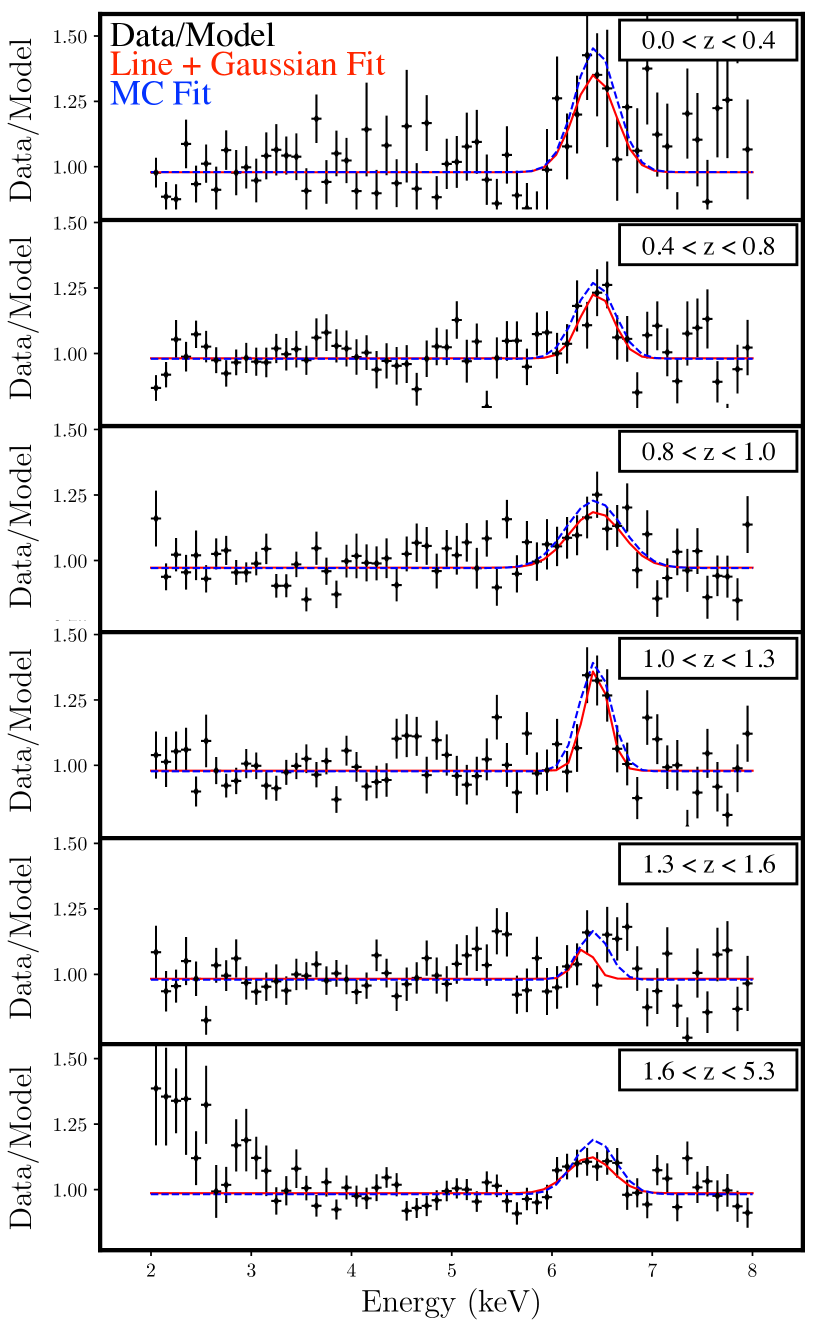
Figure 13: Data/Model ratio broken into bins of redshift.

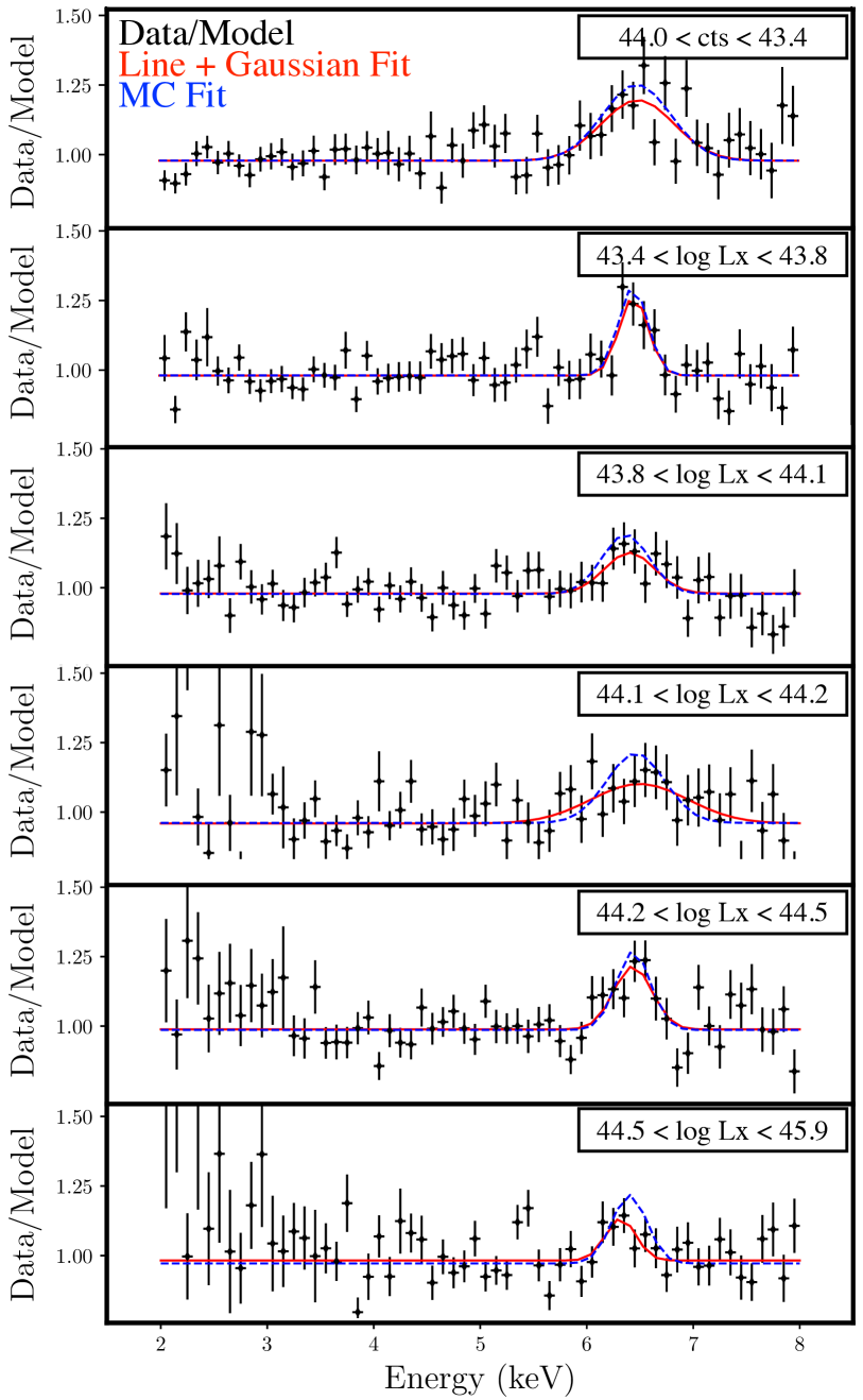
Figure 14: Data/Model ratio broken into bins of $2-10$ keV X-ray luminosity.

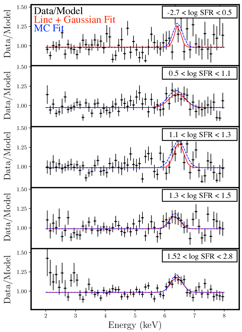
Figure 15: Data/Model ratio broken into bins of star formation rate.

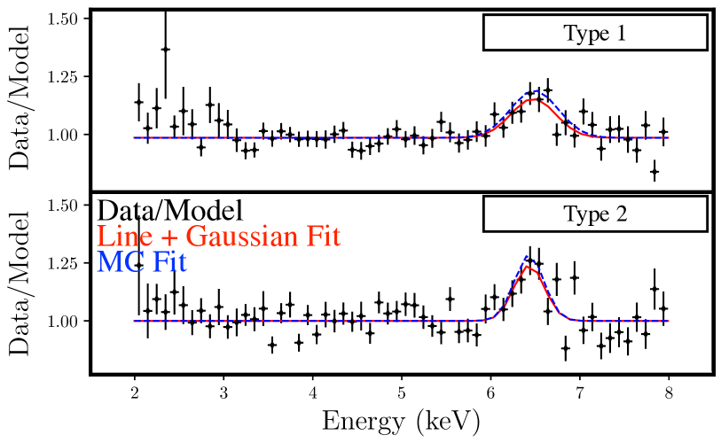
Figure 16: Data/Model ratio broken into bins of AGN Type.

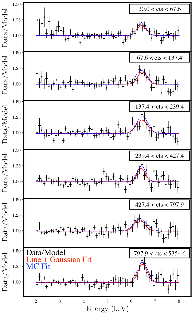
Figure 17: Data/Model ratio broken into bins of counts.

A.2 Relativistic Broadened Line

We have appended the data/model ratio fits for which we used diskline (Figure 18), relline (Figure 19, 20), and the more complex relline + Gaussian models (Figure 21, 22, 23) for the range of parameter space that was explored in our fits.

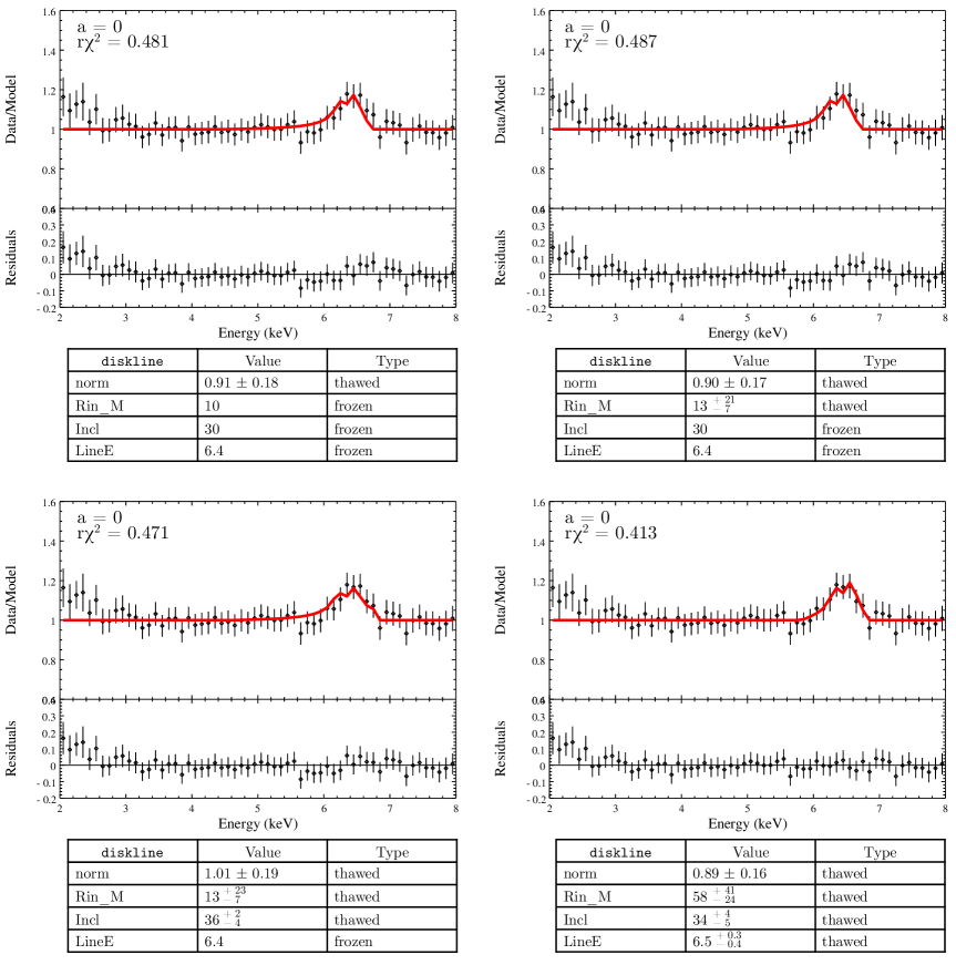
Figure 18: diskline model fits ($a=0$) to the average data/model ratio for all CCLS sources. The line energy is fixed at 6.4 keV, while all other fixed parameters are frozen at default values, unless otherwise indicated. We sequentially thaw parameters to probe this diskline model: (top, left) normalization thawed; (top, right) normalization and inner radius (Rin_M) thawed; (bottom, left) normalization, inner radius, and inclination thawed; (bottom, right) normalization, inner radius, inclination, and line energy thawed.

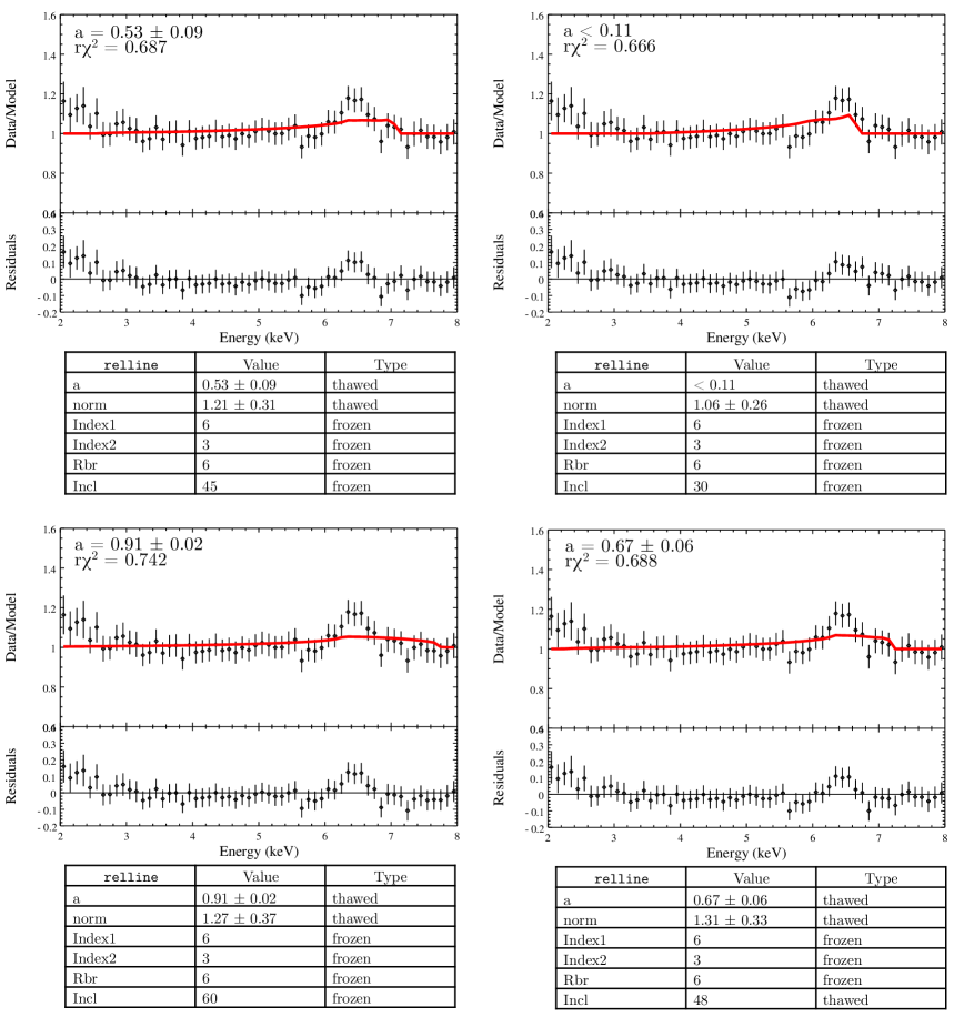
Figure 19: relline model fits to the average data/model ratio for all CCLS sources. The line energy is fixed at 6.4 keV while all other fixed parameters are frozen at default values, unless otherwise indicated. The spin parameter (a) and the normalization are left free to vary while the inclination is fixed to: (top, left) 45 degrees; (top, right) 30 degrees; (bottom, left) 60 degrees. We also allow the inclination to vary (bottom, right).

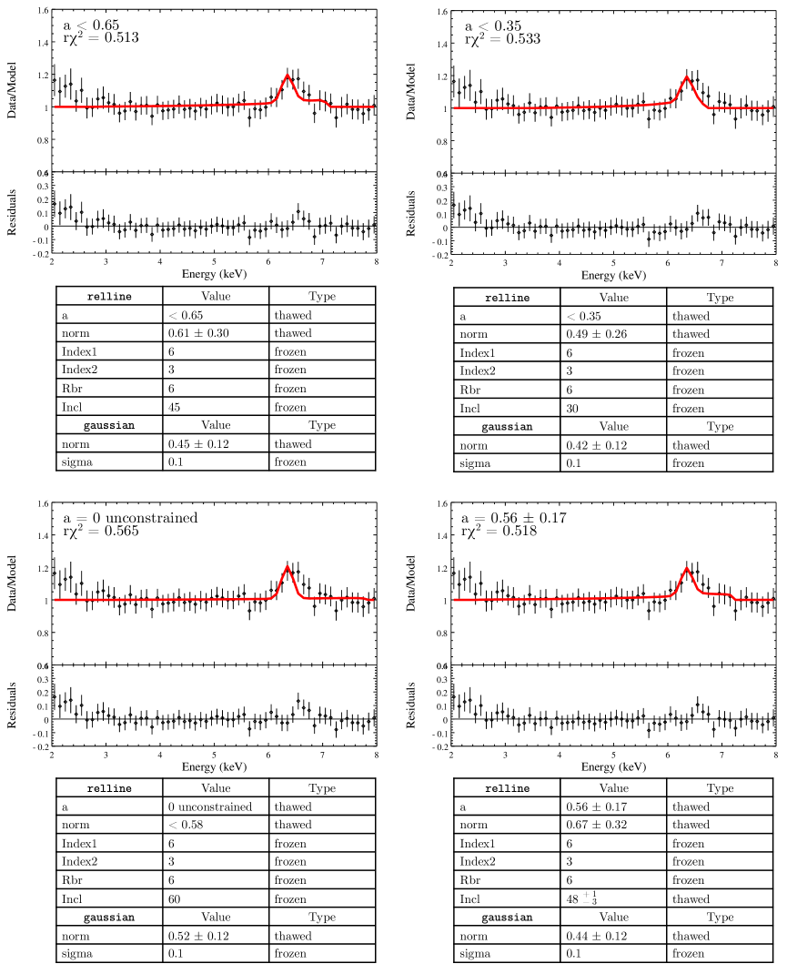
Figure 21: relline+gaussian model fits to the average data/model ratio for all CCLS sources. The relline and gaussian line energy are fixed at 6.4 keV, and the gaussian width is fixed to 0.1 keV (the size of our bins). All other fixed parameters are frozen at default values, unless otherwise indicated. The spin parameter (a) and the normalization of both the relline and gaussian are left free to vary while the inclination is fixed to: (top, left) 45 degrees; (top, right) 30 degrees; (bottom, left) 60 degrees. We also allow the inclination to vary (bottom, right).

References

- Berti & Volonteri (2008) Berti, E., & Volonteri, M. 2008, ApJ, 684, 822, doi: 10.1086/590379
- Bonson & Gallo (2016) Bonson, K., & Gallo, L. C. 2016, MNRAS, 458, 1927, doi: 10.1093/mnras/stw466
- Brenneman (2013) Brenneman, L. 2013, Acta Polytechnica, 53, 652
- Brenneman & Reynolds (2006) Brenneman, L. W., & Reynolds, C. S. 2006, ApJ, 652, 1028, doi: 10.1086/508146
- Brenneman & Reynolds (2009) —. 2009, ApJ, 702, 1367, doi: 10.1088/0004-637X/702/2/1367
- Brenneman et al. (2011) Brenneman, L. W., Reynolds, C. S., Nowak, M. A., et al. 2011, ApJ, 736, 103, doi: 10.1088/0004-637X/736/2/103
- Brusa et al. (2005) Brusa, M., Gilli, R., & Comastri, A. 2005, ApJ, 621, L5, doi: 10.1086/428928
- Cash (1979) Cash, W. 1979, ApJ, 228, 939, doi: 10.1086/156922
- Chaudhary et al. (2012) Chaudhary, P., Brusa, M., Hasinger, G., et al. 2012, A&A, 537, A6, doi: 10.1051/0004-6361/201117126
- Chen et al. (2013) Chen, C.-T. J., Hickox, R. C., Alberts, S., et al. 2013, ApJ, 773, 3, doi: 10.1088/0004-637X/773/1/3
- Civano et al. (2016) Civano, F., Marchesi, S., Comastri, A., et al. 2016, ApJ, 819, 62, doi: 10.3847/0004-637X/819/1/62
- Corral et al. (2011) Corral, A., Della Ceca, R., Caccianiga, A., et al. 2011, A&A, 530, A42, doi: 10.1051/0004-6361/201015227
- Corral et al. (2008) Corral, A., Page, M. J., Carrera, F. J., et al. 2008, A&A, 492, 71, doi: 10.1051/0004-6361:200810168
- Dai et al. (2019) Dai, X., Steele, S., Guerras, E., Morgan, C. W., & Chen, B. 2019, ApJ, 879, 35, doi: 10.3847/1538-4357/ab1d56
- Dauser et al. (2014) Dauser, T., Garcia, J., Parker, M. L., Fabian, A. C., & Wilms, J. 2014, MNRAS, 444, L100, doi: 10.1093/mnrasl/slu125
- Dauser et al. (2013) Dauser, T., Garcia, J., Wilms, J., et al. 2013, MNRAS, 430, 1694, doi: 10.1093/mnras/sts710
- Dauser et al. (2010) Dauser, T., Wilms, J., Reynolds, C. S., & Brenneman, L. W. 2010, MNRAS, 409, 1534, doi: 10.1111/j.1365-2966.2010.17393.x
- Del Moro et al. (2017) Del Moro, A., Alexander, D. M., Aird, J. A., et al. 2017, ApJ, 849, 57, doi: 10.3847/1538-4357/aa9115
- Dovčiak et al. (2004) Dovčiak, M., Karas, V., & Yaqoob, T. 2004, ApJS, 153, 205, doi: 10.1086/421115
- Fabbiano et al. (2019) Fabbiano, G., Siemiginowska, A., Paggi, A., et al. 2019, ApJ, 870, 69, doi: 10.3847/1538-4357/aaf0a4
- Fabian et al. (1989) Fabian, A. C., Rees, M. J., Stella, L., & White, N. E. 1989, MNRAS, 238, 729, doi: 10.1093/mnras/238.3.729
- Fabian et al. (2003) Fabian, A. C., Sanders, J. S., Allen, S. W., et al. 2003, MNRAS, 344, L43, doi: 10.1046/j.1365-8711.2003.06902.x
- Fabian et al. (2006) Fabian, A. C., Sanders, J. S., Taylor, G. B., et al. 2006, MNRAS, 366, 417, doi: 10.1111/j.1365-2966.2005.09896.x
- Falocco et al. (2014) Falocco, S., Carrera, F. J., Barcons, X., Miniutti, G., & Corral, A. 2014, A&A, 568, A15, doi: 10.1051/0004-6361/201322812
- Falocco et al. (2012) Falocco, S., Carrera, F. J., Corral, A., et al. 2012, A&A, 538, A83, doi: 10.1051/0004-6361/201117965
- Falocco et al. (2013) —. 2013, A&A, 555, A79, doi: 10.1051/0004-6361/201321083
- Ferrarese & Merritt (2000) Ferrarese, L., & Merritt, D. 2000, ApJ, 539, L9, doi: 10.1086/312838
- García et al. (2014) García, J., Dauser, T., Lohfink, A., et al. 2014, ApJ, 782, 76, doi: 10.1088/0004-637X/782/2/76
- George & Fabian (1991) George, I. M., & Fabian, A. C. 1991, MNRAS, 249, 352, doi: 10.1093/mnras/249.2.352
- Guainazzi et al. (2006) Guainazzi, M., Bianchi, S., & Dovčiak, M. 2006, Astronomische Nachrichten, 327, 1032, doi: 10.1002/asna.200610687
- Hopkins & Elvis (2010) Hopkins, P. F., & Elvis, M. 2010, MNRAS, 401, 7, doi: 10.1111/j.1365-2966.2009.15643.x
- Hopkins et al. (2012) Hopkins, P. F., Quataert, E., & Murray, N. 2012, MNRAS, 421, 3522, doi: 10.1111/j.1365-2966.2012.20593.x
- Iwasawa & Taniguchi (1993) Iwasawa, K., & Taniguchi, Y. 1993, ApJ, 413, L15, doi: 10.1086/186948
- Iwasawa et al. (2012) Iwasawa, K., Mainieri, V., Brusa, M., et al. 2012, A&A, 537, A86, doi: 10.1051/0004-6361/201118203
- Kalberla et al. (2005) Kalberla, P. M. W., Burton, W. B., Hartmann, D., et al. 2005, A&A, 440, 775, doi: 10.1051/0004-6361:20041864
- Lanzuisi et al. (2018) Lanzuisi, G., Civano, F., Marchesi, S., et al. 2018, MNRAS, 480, 2578, doi: 10.1093/mnras/sty2025
- Laor (1991) Laor, A. 1991, ApJ, 376, 90, doi: 10.1086/170257
- Liu et al. (2016) Liu, Z., Merloni, A., Georgakakis, A., et al. 2016, MNRAS, 459, 1602, doi: 10.1093/mnras/stw753
- Marchesi et al. (2016a) Marchesi, S., Civano, F., Elvis, M., et al. 2016a, ApJ, 817, 34, doi: 10.3847/0004-637X/817/1/34
- Marchesi et al. (2016b) Marchesi, S., Lanzuisi, G., Civano, F., et al. 2016b, ApJ, 830, 100, doi: 10.3847/0004-637X/830/2/100
- Merloni et al. (2014) Merloni, A., Bongiorno, A., Brusa, M., et al. 2014, MNRAS, 437, 3550, doi: 10.1093/mnras/stt2149
- Morganti (2017) Morganti, R. 2017, Frontiers in Astronomy and Space Sciences, 4, 42, doi: 10.3389/fspas.2017.00042
- Pacucci & Loeb (2020) Pacucci, F., & Loeb, A. 2020, ApJ, 895, 95, doi: 10.3847/1538-4357/ab886e
- Reis et al. (2014) Reis, R. C., Reynolds, M. T., Miller, J. M., & Walton, D. J. 2014, Nature, 507, 207, doi: 10.1038/nature13031
- Reynolds (2014) Reynolds, C. S. 2014, Space Sci. Rev., 183, 277, doi: 10.1007/s11214-013-0006-6
- Reynolds (2019) —. 2019, Nature Astronomy, 3, 41, doi: 10.1038/s41550-018-0665-z
- Reynolds et al. (2012) Reynolds, C. S., Brenneman, L. W., Lohfink, A. M., et al. 2012, ApJ, 755, 88, doi: 10.1088/0004-637X/755/2/88
- Stemo et al. (2020) Stemo, A., Comerford, J. M., Barrows, R. S., et al. 2020, ApJ, 888, 78, doi: 10.3847/1538-4357/ab5f66
- Suh et al. (2020) Suh, H., Civano, F., Trakhtenbrot, B., et al. 2020, ApJ, 889, 32, doi: 10.3847/1538-4357/ab5f5f
- Suh et al. (2019) Suh, H., Civano, F., Hasinger, G., et al. 2019, ApJ, 872, 168, doi: 10.3847/1538-4357/ab01fb
- Vasudevan et al. (2016) Vasudevan, R. V., Fabian, A. C., Reynolds, C. S., et al. 2016, MNRAS, 458, 2012, doi: 10.1093/mnras/stw363
- Walton et al. (2015) Walton, D. J., Reynolds, M. T., Miller, J. M., et al. 2015, ApJ, 805, 161, doi: 10.1088/0004-637X/805/2/161
- Yang et al. (2019) Yang, G., Brandt, W. N., Alexander, D. M., et al. 2019, MNRAS, 485, 3721, doi: 10.1093/mnras/stz611
- Yang et al. (2018) Yang, G., Brandt, W. N., Darvish, B., et al. 2018, MNRAS, 480, 1022, doi: 10.1093/mnras/sty1910
- Yaqoob & Padmanabhan (2004) Yaqoob, T., & Padmanabhan, U. 2004, ApJ, 604, 63, doi: 10.1086/381731
- Zappacosta et al. (2018) Zappacosta, L., Comastri, A., Civano, F., et al. 2018, ApJ, 854, 33, doi: 10.3847/1538-4357/aaa550