Iterations of symplectomorphisms and $p$-adic analytic actions on Fukaya category

Abstract.

Inspired by the work of Bell on dynamical Mordell-Lang conjecture, and by the family Floer homology, we construct $p$-adic analytic families of bimodules on the Fukaya category of a monotone or negatively monotone symplectic manifold, interpolating the bimodules corresponding to iterates of a symplectomorphism $\phi$ isotopic to identity. We consider this family as a $p$-adic analytic action on the Fukaya category. Using this, we deduce that the ranks of Floer homology groups $HF(\phi^{k}(L),L^{\prime};\Lambda)$ are constant in $k\in{\mathbb{Z}}$, with finitely many possible exceptions. We also prove an analogous result without the monotonicity assumption for generic $\phi$ isotopic to identity by showing how to construct a $p$-adic analytic action in this case.

1. Introduction

1.1. Motivation and main results

In [Bel06], Bell proves the following theorem: let $Y$ be an affine variety over a field of characteristic $0$ and $f:Y\to Y$ be an automorphism. Consider a subvariety $X\subset Y$ and a point $x\in Y$. Then, the set $\{n\in{\mathbb{N}}:f^{n}(x)\in X\}$ is a union of finitely many arithmetic progressions and a set of finitely many numbers. In [Sei16], Seidel conjectures a symplectic version of this statement. Namely, given symplectic manifold $(M,\omega_{M})$, a symplectomorphism $\phi$ and two Lagrangians $L,L^{\prime}\subset M$ (for which Floer homology is well-defined), the set

(1.1) $$\{n\in{\mathbb{N}}:f^{n}(L)\text{ and }L^{\prime}\text{ are Floer theoretically isomorphic}\}$$

form a union of finitely many arithmetic progressions and a set of finitely many numbers.

The purpose of this paper is to prove a version of this statement when $\phi\in Symp^{0}(M,\omega_{M})$, i.e. $\phi$ is isotopic to identity through symplectomorphisms. Our main theorem holds when $(M,\omega_{M})$ is monotone or negatively monotone. Namely:

Theorem 1.1.

Assume $(M,\omega_{M})$ is a symplectic manifold and $L,L^{\prime}\subset M$ are monotone Lagrangians such that Assumption 1.2 is satisfied. Then, the rank of $HF(\phi^{k}(L),L^{\prime};\Lambda)$ is constant except for finitely many $k$.

Here, $HF(L,L^{\prime};\Lambda)$ denotes the Lagrangian Floer homology group defined with coefficients in the Novikov field $\Lambda={\mathbb{Q}}((T^{\mathbb{R}}))$. We will sometimes omit $\Lambda$ from the notation and denote this group by $HF(L,L^{\prime})$.

Assumption 1.2.

The monotone Fukaya category ${\mathcal{F}}(M;\Lambda)$ is smooth, and it is generated by a set of Lagrangians $L_{1},\dots,L_{m}$ with minimal Maslov number at least $3$ satisfying either

• image of $\pi_{1}(L_{i})\to\pi_{1}(M)$ is torsion

• $L_{i}$ is Bohr-Sommerfeld monotone

Also, $L,L^{\prime}$ have minimal Maslov number at least $3$ and they are also Bohr-Sommerfeld monotone in the latter case.

We assume $L$ and $L^{\prime}$ are Bohr-Sommerfeld as the proof is more geometric in this case; however, as we will explain at the end of Section 4, this assumption can be dropped. We should also note that in the examples we have $L_{i}$ satisfy the latter assumption and not the former.

Example 1.3.

One can let $M=\Sigma_{g}$ to be a surface of genus greater than or equal to $2$. Finite generation of ${\mathcal{F}}(\Sigma_{g},\Lambda)$ is shown in [Sei11] and [Efi12], and that this category is homologically smooth follows from the fact that matrix factorization categories are homologically smooth (see [Dyc11]). Alternatively see [AS20, Lemma 2.18]. That one can let generators to be Bohr-Sommerfeld monotone follows from the fact that every non-separating curve has such a representative in its isotopy class (see [Sei11], note the author uses the term balanced for Bohr-Sommerfeld monotone). Let $\ell_{1}\subset\Sigma_{g}$ be a non-separating simple closed curve with primitive homology class in $\Sigma_{g}$ (in particular it is not null-homologous). One can let $\ell_{1}$ to be one of the meridians in a decomposition $\Sigma_{g}=(T^{2})^{\#g}$. Let $\phi$ be a symplectomorphism with small flux that disjoints $\ell_{1}$ from itself and let $\ell_{2}=\phi(\ell_{1})$, $\ell_{3}=\phi^{2}(\ell_{1})$ (also assume $\ell_{1}\cap\ell_{3}=\emptyset$). Consider $L=\ell_{1}$ and $L^{\prime}=\ell_{2}\cup\ell_{3}$ equipped with Spin structures. Applying Theorem 1.1, we see that the rank of $HF(\phi^{k}(L),L^{\prime};\Lambda)$ is constant except finitely many $k$. In this example, the finite exceptional set is $k=1,2$. Note $\ell_{2}\cup\ell_{3}$ cannot be Bohr-Sommerfeld monotone.

Example 1.4.

Let $M=\Sigma_{2}\times\Sigma_{2}$. In addition to $\ell_{1},\ell_{2},\ell_{3}$ consider a non-separating curve $\ell\subset\Sigma_{2}$ with primitive homology class, that is fixed by $\phi$, and that intersect each of $\ell_{1}$, $\ell_{2}$ and $\ell_{3}$ exactly at one point. Let $\phi^{\prime}=\phi\times\phi$. Consider the Lagrangian tori $\ell_{1}\times\ell$ and $\ell\times\ell_{1}$. These tori intersect at one point, defining a morphism $\ell_{1}\times\ell\to\ell\times\ell_{1}$ (of non-zero degree possibly). Let $L$ be a Lagrangian representing the cone of this morphism, which can be obtained by Lagrangian surgery. We let $L^{\prime}=\ell_{2}\times\ell_{3}$. Clearly, $\phi^{\prime-k}(L^{\prime})$ has non-vanishing Floer homology with $\ell_{1}\times\ell$ only when $k=1$ and with $\ell\times\ell_{1}$ only when $k=2$. Therefore, $HF(\phi^{\prime k}(L),L^{\prime};\Lambda)$ is non-zero only at $k=1,2$. One can produce examples with more sophisticated finite sets of exceptional $k$ in this way. Presumably, the images of $L$ and $\ell_{1}\times\ell\cup\ell\times\ell_{1}$ in $Sym^{2}(\Sigma_{2})$ also illustrate a case when the rank jumps twice.

To define Bohr-Sommerfeld monotonicity, we need to fix some data on $M$. See [Sei11] for the case of higher genus surfaces and [WW10] for more general manifolds. Throughout the paper, we use the word monotone to refer to both monotone and negatively monotone. In other words, $(M,\omega_{M})$ is monotone if $[c_{1}(M)]=\lambda[\omega_{M}]$, for some $\lambda\neq 0$. Under Assumption 1.2, the counts of marked discs defining the Fukaya category with objects $L_{i}$ are finite (see [Oh93], [She16], [WW10]); therefore, the Fukaya category can be defined over the field of Novikov polynomials. Let ${\mathcal{F}}(M,\Lambda)$ denote the Fukaya category spanned by $L_{i}$ that is defined over the Novikov field $\Lambda={\mathbb{Q}}((T^{\mathbb{R}}))$. One can define the Fukaya category over a field extension of ${\mathbb{Q}}$ that is generated by $\{T^{E(u)}\}$, where $u$ ranges over marked pseudo-holomorphic discs with boundary on $L_{i}$ and asymptotic to intersection points. The set of all possible energies is in the span of a finitely generated subgroup $G\subset{\mathbb{R}}$; therefore, the extension of ${\mathbb{Q}}$ by all such $T^{E(u)}$ is in a finitely generated extension of ${\mathbb{Q}}$ by elements of the form $T^{g},g\in G$. In other words, the Fukaya category can be defined over a finitely generated field extension of ${\mathbb{Q}}$ generated by such elements. Moreover, Assumption 1.2 implies disc counts defining the Yoneda modules $h^{L},h_{L^{\prime}}$ are also finite and by adding energies of these into $G\subset{\mathbb{R}}$, we can ensure these modules are also defined over the Fukaya category with coefficients in the finitely generated extension above. Fix brane structures, as well as Floer data to define the Fukaya category and these modules (see [Sei08] for definitions).

After the proof of Theorem 1.1, we seek ways to drop the assumption of monotonicity. We do not expect Theorem 1.1 to hold in general; for instance, for $M=T^{2}$ with a fixed area form, there exists one periodic symplectic flows on $M$ with non-zero flux. More specifically, if $\ell\subset T^{2}$ is a meridian, one can let $\phi$ to be the rotation of $T^{2}$ in the orthogonal direction by $\pi/3$. Then, $HF(\phi^{k}(\ell),\ell;\Lambda)$ is not constant in $k$ even after finitely many $k$, although it is still periodic. However, one can still prove the following:

Theorem 1.5.

Assume $(M,\omega_{M})$ is a symplectic manifold with two Lagrangian branes $L,L^{\prime}\subset\Lambda$ satisfying Assumption 1.6. Given generic $\phi\in Symp^{0}(M,\omega_{M})$, the rank of $HF(\phi^{k}(L),L^{\prime};\Lambda)$ is constant in $k\in{\mathbb{Z}}$ with finitely many possible exceptions.

By generic, we mean that the flux of an isotopy from $1$ to $\phi$ is generic. This will be explained further in this section and in Section 5.

Assumption 1.6.

${\mathcal{F}}(M,\Lambda)$ is an (uncurved, ${\mathbb{Z}}$ or ${\mathbb{Z}}/2{\mathbb{Z}}$-graded) $A_{\infty}$-category over $\Lambda$, it is smooth and proper, generated by $L_{1},\dots,L_{m}$. Also, $L,L^{\prime}$ are Lagrangians with brane structure that bound no Maslov $2$ discs (so they define objects of Fukaya category).

We let ${\mathcal{F}}(M,\Lambda)$ denote the category spanned by the generators $L_{1},\dots,L_{m}$, as before. Theorem 1.5 is valid in great generality. As examples of such $M$, one can consider $T^{2}$ and $T^{2}\times T^{2}$.

Remark 1.7.

Bell’s theorem mentioned at the beginning is a case of the dynamical Mordell-Lang conjecture. In [BSS17], the authors prove a version of this conjecture for coherent sheaves. Theorem 1.1 and Theorem 1.5 are closer to this statement in spirit. Note however, our techniques extend to prove a statement that is closer to Seidel’s conjecture: namely, under Assumption 1.2, $k\in{\mathbb{N}}$ such that $\phi^{k}(L)$ and $L^{\prime}$ are stably Floer theoretically isomorphic form a set that is either finite or cofinite (hence either a singleton or everything). By stably isomorphic, we mean $L$ is a direct summand of $L^{\prime\oplus q}$, for some $q\gg 0$, and vice versa. An immediate corollary of this is if $\phi^{k}(L)$ is Hamiltonian isotopic to $L^{\prime}$ for two different $k$, then it is stably isomorphic for all $k$. Let $\alpha$ be a closed $1$-form such that $\phi=\phi_{\alpha}^{1}$. By replacing $\phi$ by $\phi_{\alpha}^{1/n}$, where $n\in{\mathbb{N}}$, we see that $\phi_{\alpha}^{k/n}(L)$ is stably isomorphic to $L^{\prime}$ for all $k$; therefore, $\phi_{\alpha}^{f}(L)$ and $L^{\prime}$ are stably isomorphic for $f\in{\mathbb{Q}}$. One can presumably show that for small $t\in{\mathbb{R}}$, $HF(L,\phi_{\alpha}^{t}(L))=0$; hence, $L$ and $\phi_{\alpha}^{t}(L)$ are not stably isomorphic unless $\alpha|_{L}=0$. This implies $\phi_{\alpha}^{t}(L)$ is Hamiltonian isotopic to $L^{\prime}$ for all $t$.

1.2. Summary of the proofs

Fix a path from $1_{M}$ to $\phi$ through symplectomorphisms and assume the flux of the path is $\alpha$ where $\alpha$ is a closed $1$-form. Every closed $1$-form generates a symplectic isotopy $\phi_{\alpha}^{t}$ as the flow of vector field $X_{\alpha}$ satisfying $\omega(\cdot,X_{\alpha})=\alpha$ and $\phi^{1}_{\alpha}$ is Hamiltonian isotopic to $\phi$ by Banyaga’s theorem. Therefore, the action of $\phi$ and $\phi^{1}_{\alpha}$ on Floer homology are the same and we may assume $\phi=\phi^{1}_{\alpha}$. The isotopy $\phi_{\alpha}^{t}$ generate a family of bimodules by:

(1.2) $$(L_{i},L_{j})\mapsto HF(\phi^{t}_{\alpha}(L_{i}),L_{j})$$

We give a quasi-isomorphic description of this family inspired by family Floer homology (see [Abo14]) and quilted Floer homology (as in [Ma’15], [Gan12]). The simplest version is the following: consider the ring ${\mathbb{Q}}(T^{\mathbb{R}})[z^{\mathbb{R}}]$. To every pair of Lagrangians, associate

(1.3) $$(L_{i},L_{j})\mapsto\mathfrak{M}^{\Lambda}_{\alpha}(L_{i},L_{j})=CF(L_{i},L_{j})\otimes{\mathbb{Q}}(T^{\mathbb{R}})[z^{\mathbb{R}}]$$

with differential given by

(1.4) $$x\mapsto\sum\pm T^{E(u)}z^{\alpha([\partial_{h}u])}.y$$

where the sum ranges over pseudo-holomorphic strips from $x$ to $y$ and $[\partial_{h}u]$ denotes the class of “one side of the boundary of $u$”. When, $L_{i}$ satisfy the condition that $Im(\pi_{1}(L_{i})\to\pi_{1}(M))$ are torsion, these $z$-terms are actually $1$. However, one can define the higher structure maps of the bimodule by the rule

(1.5) $$(x_{1},\dots,x_{k}|x|x_{1}^{\prime},\dots,x_{l}^{\prime})\mapsto\sum\pm T^{E(u)}z^{\alpha([\partial_{h}u])}.y$$

where the sum ranges over pseudo-holomorphic marked discs with input $x_{1},\dots,y,\dots x_{l}^{\prime}$ and output $y$. Without the $z$-term, this is just the definition of $A_{\infty}$-structure maps, and the count is finite by monotonicity. $[\partial_{h}u]\in H_{1}(M,{\mathbb{Z}})$ denotes the “part of boundary of disc $u$” from the bimodule input $x$ to output $y$ (see also Figure 3.1. For a precise definition of the class $[\partial_{h}u]$, we will fix a base point on $M$ and homotopy classes of paths from this base point to generators of Floer homology groups). Now, the $z$-term does not have to be trivial, and this gives a deformation of the diagonal bimodule of ${\mathcal{F}}(M)$. That the maps (1.5) satisfy the $A_{\infty}$-bimodule equation is immediate. Moreover, it is possible to show this gives the bimodule corresponding to $\phi^{f}_{\alpha}$, when we plug $z=T^{f}$ for small $f\in{\mathbb{R}}$. There are no convergence issues as in [Abo14] as the count is finite, but for larger $f$, the bimodule $\mathfrak{M}^{\Lambda}_{\alpha}|_{z=T^{f}}$ has no a priori relation to $\phi_{\alpha}^{f}$. On the other hand, one can show that for any Lagrangian brane $\tilde{L}$, the Yoneda modules satisfy

(1.6) $$h_{\phi_{\alpha}^{f}(\tilde{L})}\simeq h_{\tilde{L}}\otimes_{{\mathcal{F}}(M,\Lambda)}\mathfrak{M}^{\Lambda}_{\alpha}|_{z=T^{f}}$$

when $|f|$ is small (we use $|f|$ to denote ordinary absolute value). Similarly, if $|f|$ and $|f^{\prime}|$ are small, then

(1.7) $$\mathfrak{M}^{\Lambda}_{\alpha}|_{z=T^{f+f^{\prime}}}\simeq\mathfrak{M}^{\Lambda}_{\alpha}|_{z=T^{f}}\otimes_{{\mathcal{F}}(M,\Lambda)}\mathfrak{M}^{\Lambda}_{\alpha}|_{z=T^{f^{\prime}}}$$

See Lemma 4.6 and Lemma 3.5 respectively. For arbitrary, $f>0$, there exists a sequence of numbers $0=s_{0}<s_{1}<\dots<s_{r}=f$ such that

(1.8) $$h_{\phi^{f}_{\alpha}(\tilde{L})}\simeq h_{\tilde{L}}\otimes_{{\mathcal{F}}(M,\Lambda)}\mathfrak{M}_{(s_{1}-s_{0})\alpha}^{\Lambda}\otimes_{{\mathcal{F}}(M,\Lambda)}\mathfrak{M}_{(s_{2}-s_{1})\alpha}^{\Lambda}\dots\otimes_{{\mathcal{F}}(M,\Lambda)}\mathfrak{M}_{(s_{r}-s_{r-1})\alpha}^{\Lambda}$$

Similarly, for $f<0$, there exists $0=s_{0}>s_{1}>\dots>s_{r}=f$ such that (1.8) holds.

Above we mentioned that Fukaya category can be defined over ${\mathbb{Q}}(T^{g}:g\in G)$, where $G$ is a finitely generated additive subgroup of ${\mathbb{R}}$ containing all possible energies of pseudo-holomorphic discs. Without loss of generality add $\alpha(H_{1}(M,{\mathbb{Z}}))$ into $G$, then the coefficients defining (1.4) would be in ${\mathbb{Q}}(T^{g}:g\in G)$, and one can “evaluate” (1.4) at $z=T^{f}$, for $f\in{\mathbb{Z}}$. In other words, one can define a similar family $\mathfrak{M}^{K}_{\alpha}$ over ${\mathcal{F}}(M,K)$- the Fukaya category with coefficients over $K$, where $K\subset{\mathbb{Q}}((T^{\mathbb{R}}))$ is a field containing ${\mathbb{Q}}(T^{g}:g\in G)$. We will add some roots of $T^{\alpha(C)}$ to $K$.

Let $p>2$ be prime and consider the purely transcendental field extension ${\mathbb{Q}}(T^{g}:g\in G)$. By choosing a finite number of elements from $1+p{\mathbb{Z}}_{p}$ that satisfy no algebraic relation over ${\mathbb{Q}}$, one can find an embedding of ${\mathbb{Q}}(T^{g}:g\in G)$ into ${\mathbb{Q}}_{p}$ such that $T^{g}\mapsto 1+p{\mathbb{Z}}_{p}$. Moreover, as we will see in bigger generality, for any $f\in{\mathbb{Z}}_{(p)}=\{\frac{a}{b}:a,b\in{\mathbb{Z}},p\nmid b\}$, and $v\in 1+p{\mathbb{Z}}_{p}$, one can define a canonical $f^{th}$ root via

(1.9) $$v^{f}=\sum_{i=0}^{\infty}{f\choose i}(v-1)^{i}\in 1+p{\mathbb{Z}}_{p}$$

Therefore, we can write a field homomorphism

(1.10) $$\mu:K:={\mathbb{Q}}(T^{g/b}:g\in G,p\nmid b\in{\mathbb{Z}})\to{\mathbb{Q}}_{p}$$

that sends $T^{g/b}$ into $1+p{\mathbb{Z}}_{p}$. Denote the image of $T^{g/b}$ by $T_{\mu}^{g/b}$.

It is easy to see that the exponentiation (1.9) extends to an element $v^{t}\in{\mathbb{Q}}_{p}\langle t\rangle$ simply by replacing $f$ by $t$. ${\mathbb{Q}}_{p}\langle t\rangle$ is the Tate algebra and it can be thought as the analytic functions on $p$-adic unit disc ${\mathbb{Z}}_{p}$. Therefore, one can define a $p$-adic family of bimodules exactly in the same way, except we replace formula (1.5) by

(1.11) $$(x_{1},\dots,x_{k}|x|x_{1}^{\prime},\dots,x_{l}^{\prime})\mapsto\sum\pm T_{\mu}^{E(u)}T_{\mu}^{t\alpha([\partial_{h}u])}.y$$

We denote this family by $\mathfrak{M}^{{\mathbb{Q}}_{p}}_{\alpha}$ and think of it as an “analytic map from ${\mathbb{Z}}_{p}$ to auto-equivalence group of the Fukaya category”. Our first claim is that this map behaves like a group homomorphism on a ($p$-adically) small neighborhood $p^{n}{\mathbb{Z}}_{p}\subset{\mathbb{Z}}_{p}$ of $0$. In other words, it is group-like. More precisely, there exists a morphism

(1.12) $$\pi_{1}^{*}\mathfrak{M}_{\alpha}^{{\mathbb{Q}}_{p}}\otimes\pi_{2}^{*}\mathfrak{M}_{\alpha}^{{\mathbb{Q}}_{p}}\to\Delta^{*}\mathfrak{M}_{\alpha}^{{\mathbb{Q}}_{p}}$$

of families over ${\mathbb{Q}}_{p}\langle t_{1},t_{2}\rangle$ that induce a quasi-isomorphism on a small neighborhood of $t_{1}=t_{2}=0$. To explain the notation, we identify ${\mathbb{Q}}_{p}\langle t_{1},t_{2}\rangle$ with (completed) tensor product of ${\mathbb{Q}}_{p}\langle t\rangle$ with itself. Then $\pi_{k}$ correspond to projection maps and $\Delta$ to group multiplication for the group $Sp({\mathbb{Q}}_{p}\langle t\rangle)$ (note that we make no formal reference to affinoid domain and work entirely with Tate algebra, which is also a Hopf algebra in this case, $\Delta$ is the coproduct map). The map (1.12) induces a well known quasi-isomorphism at $t_{1}=t_{2}=0$ and the semi-continuity property of quasi-isomorphisms imply the same in a small $p$-adic neighborhood. This proves that $\mathfrak{M}_{\alpha}^{{\mathbb{Q}}_{p}}$ is group-like after base change under ${\mathbb{Q}}_{p}\langle t\rangle\subset{\mathbb{Q}}_{p}\langle t/p^{n}\rangle$. The latter can be seen as the algebra of analytic functions on $p^{n}{\mathbb{Z}}_{p}$, and one can heuristically think of $\mathfrak{M}^{{\mathbb{Q}}_{p}}_{\alpha}|_{{\mathbb{Q}}_{p}\langle t/p^{n}\rangle}$ as a $Sp({\mathbb{Q}}_{p}\langle t/p^{n}\rangle)$ action on ${\mathcal{F}}(M,{\mathbb{Q}}_{p})$. One can presumably show the group-like property over ${\mathbb{Q}}_{p}\langle t\rangle$ using deformation class computations as in [Sei14], [Kar18]; however, we do not follow this way. Note that the ${\mathcal{F}}(M,K)$-bimodule $\mathfrak{M}^{K}_{\alpha}|_{z=T^{f}}$ base changes to $\mathfrak{M}^{{\mathbb{Q}}_{p}}_{\alpha}|_{t=f}$, for any $f\in{\mathbb{Z}}_{(p)}$; therefore,

(1.13) $$\mathfrak{M}^{K}_{\alpha}|_{z=T^{f+f^{\prime}}}\simeq\mathfrak{M}^{K}_{\alpha}|_{z=T^{f}}\otimes_{{\mathcal{F}}(M,K)}\mathfrak{M}^{K}_{\alpha}|_{z=T^{f^{\prime}}}\atop\mathfrak{M}^{\Lambda}_{\alpha}|_{z=T^{f+f^{\prime}}}\simeq\mathfrak{M}^{\Lambda}_{\alpha}|_{z=T^{f}}\otimes_{{\mathcal{F}}(M,\Lambda)}\mathfrak{M}^{\Lambda}_{\alpha}|_{z=T^{f^{\prime}}}$$

for any $f,f^{\prime}\in p^{n}{\mathbb{Z}}_{(p)}=\{\frac{a}{b}:a,b\in{\mathbb{Z}},p^{n}|a,p\nmid b\}$ (i.e. when $f$ and $f^{\prime}$ are $p$-adically small).

When $f\in p^{n}{\mathbb{Z}}_{(p)}$, one can choose $0=s_{0}<s_{1}<\dots<s_{r}=f$ in (1.8) such that all $s_{i}\in p^{n}{\mathbb{Z}}_{(p)}$. Therefore, by letting $\tilde{L}=L^{\prime}$ and using (1.13), we see that

(1.14) $$h_{\phi^{f}_{\alpha}(L^{\prime})}\simeq h_{L^{\prime}}\otimes_{{\mathcal{F}}(M,\Lambda)}\mathfrak{M}^{\Lambda}_{\alpha}|_{z=T^{f}}$$

By replacing $f$ by $-f$ and applying $\otimes_{{\mathcal{F}}(M,\Lambda)}h^{L}$ on the right, we obtain

(1.15) $$CF(L,\phi^{-f}_{\alpha}(L^{\prime}))\simeq h_{\phi^{-f}_{\alpha}(L^{\prime})}\otimes_{{\mathcal{F}}(M,\Lambda)}h^{L}\simeq h_{L^{\prime}}\otimes_{{\mathcal{F}}(M,\Lambda)}\mathfrak{M}^{\Lambda}_{\alpha}|_{z=T^{-f}}\otimes_{{\mathcal{F}}(M,\Lambda)}h^{L}$$

By assumption, $h_{L^{\prime}}$ and $h^{L}$ are definable over ${\mathcal{F}}(M,K)$; hence,

(1.16) $$h_{L^{\prime}}\otimes_{{\mathcal{F}}(M,K)}\mathfrak{M}^{K}_{\alpha}|_{z=T^{-f}}\otimes_{{\mathcal{F}}(M,K)}h^{L}$$

is well-defined and has cohomology of dimension same as $HF(L,\phi^{-f}_{\alpha}(L^{\prime}))\cong HF(\phi^{f}_{\alpha}(L),L^{\prime})$. It also extends to

(1.17) $$h_{L^{\prime}}\otimes_{{\mathcal{F}}(M,{\mathbb{Q}}_{p})}\mathfrak{M}^{{\mathbb{Q}}_{p}}_{\alpha}|_{t={-f}}\otimes_{{\mathcal{F}}(M,{\mathbb{Q}}_{p})}h^{L}$$

under base change along $\mu:K\to{\mathbb{Q}}_{p}$.

One can show that

(1.18) $$h_{L^{\prime}}\otimes_{{\mathcal{F}}(M,{\mathbb{Q}}_{p})}\mathfrak{M}^{{\mathbb{Q}}_{p}}_{\alpha}|_{{\mathbb{Q}}_{p}\langle t/p^{n}\rangle}\otimes_{{\mathcal{F}}(M,{\mathbb{Q}}_{p})}h^{L}$$

is quasi-isomorphic to a finite complex of finitely generated ${\mathbb{Q}}_{p}\langle t/p^{n}\rangle$-modules. This implies that its cohomology has constant rank at all $f\in p^{n}{\mathbb{Z}}_{(p)}$, with finitely many exceptions. In other words, $HF(\phi^{f}_{\alpha}(L),L^{\prime})$ has constant rank among all $f\in p^{n}{\mathbb{Z}}_{(p)}$, with finitely many possible exceptions.

Choose $f_{i}\in{\mathbb{Z}}_{(p)}$ for $i=1,\dots,p^{n}-1$ such that $|f_{i}|$ is small and $f_{i}\equiv i\,(mod\,p^{n})$. We want to replace $L^{\prime}$ by $\phi_{\alpha}^{-f_{i}}(L^{\prime})$ in (1.18); however, we need definability of $h_{\phi_{\alpha}^{-f_{i}}(L^{\prime})}$ over ${\mathcal{F}}(M,K)$, thus over ${\mathcal{F}}(M,{\mathbb{Q}}_{p})$. For this purpose, we use $h^{alg}_{\phi_{\alpha}^{-f_{i}},L^{\prime}}$, an $A_{\infty}$-module over ${\mathcal{F}}(M,K)$ that becomes quasi-isomorphic to $h_{\phi_{\alpha}^{-f_{i}}(L^{\prime})}$ after extending the coefficients from $K$ to $\Lambda$ and that is obtained by an algebraic deformation of $h_{L^{\prime}}$. One can replace $h_{L^{\prime}}$ by $h^{alg}_{\phi_{\alpha}^{-f_{i}},L^{\prime}}$ in (1.18), and the same reasoning proves that the newly obtained complex has cohomology of constant rank among all $f\in p^{n}{\mathbb{Z}}_{(p)}$ with finitely many possible exceptions. In other words, $HF(L,\phi^{-f-f_{i}}_{\alpha}(L^{\prime}))\cong HF(\phi^{f+f_{i}}_{\alpha}(L),L^{\prime})$ has constant dimension for $f\in p^{n}{\mathbb{Z}}_{(p)}$, with finitely many possible exceptions. Since $\{f_{i}\}_{i}\cup\{0\}$ cover all classes modulo $p^{n}$, we can conclude that the rank of $HF(\phi^{f}_{\alpha}(L),L^{\prime})$ is $p^{n}$-periodic except finitely many, in other words, if $f,f^{\prime}\in{\mathbb{Z}}_{(p)}$, then $HF(\phi^{f}_{\alpha}(L),L^{\prime})$ and $HF(\phi^{f+p^{n}f^{\prime}}_{\alpha}(L),L^{\prime})$ has the same dimension, except possibly a finite number of $f$.

We did not have any restriction on $p>2$, and one can replace it by another prime $p^{\prime}$ to conclude that the dimension of $HF(\phi^{f}_{\alpha}(L),L^{\prime})$ is also $p^{\prime n^{\prime}}$-periodic for $f^{\prime}\in{\mathbb{Z}}_{(p^{\prime})}$, with finitely many possible exceptions. As $p^{n}$ and $p^{\prime n^{\prime}}$ are coprime, this proves that the rank of $HF(\phi^{f}_{\alpha}(L),L^{\prime})$ is constant among $f\in\mathbb{Z}$, with finitely many possible exceptions, i.e. Theorem 1.1 follows. Observe that the proof implies the constancy of dimension of $HF(\phi^{f}_{\alpha}(L),L^{\prime})$ for the dense subset ${\mathbb{Z}}_{(p)}\cap{\mathbb{Z}}_{(p^{\prime})}={\mathbb{Z}}_{(pp^{\prime})}=\{\frac{a}{b}:a,b\in{\mathbb{Z}},p\nmid b,p^{\prime}\nmid b\}$ of ${\mathbb{R}}$ with finitely many exceptions.

As mentioned above, one can actually drop the Bohr-Sommerfeld assumption on $L$ and $L^{\prime}$. For the proof to go through, we need definability of $h_{L^{\prime}}$, $h^{L}$ over ${\mathcal{F}}(M,K)$ or ${\mathcal{F}}(M,\tilde{K})$, where $\tilde{K}$ is a finitely generated extension of $K$. This may not be always possible, but as one can represent $L$ and $L^{\prime}$ as elements of $tw^{\pi}({\mathcal{F}}(M,\Lambda))$ and as the data to define a twisted complex is finite, there exists a finitely generated extension $\tilde{K}$ of $K$ inside $\Lambda$, and ${\mathcal{F}}(M,\tilde{K})$-modules $h_{L^{\prime}}^{\prime}$, $h^{\prime L}$ that become quasi-isomorphic to $h_{L^{\prime}}$ and $h^{L^{\prime}}$ after base change along $\tilde{K}\to\Lambda$. Since $\tilde{K}$ is finitely generated, one can extend $\mu:K\to{\mathbb{Q}}_{p}$ to a map $\tilde{\mu}:\tilde{K}\to{\mathbb{Q}}_{p}^{\prime}$, where ${\mathbb{Q}}_{p}^{\prime}$ is a finite (not only finitely generated) extension of ${\mathbb{Q}}_{p}$, which automatically carries a discrete valuation. This allows us to define the complex $h^{\prime}_{L^{\prime}}\otimes_{{\mathcal{F}}(M,{\mathbb{Q}}_{p}^{\prime})}\mathfrak{M}_{\alpha}^{{\mathbb{Q}}_{p}^{\prime}}\otimes_{{\mathcal{F}}(M,{\mathbb{Q}}_{p}^{\prime})}h^{\prime L}$ over ${\mathbb{Q}}_{p}^{\prime}\langle t/p^{n}\rangle$, whose rank at $t=kp^{n}$ is still $HF(\phi_{\alpha}^{-kp^{n}}(L),L^{\prime};\Lambda)$. As before, this implies that the rank of $HF(\phi_{\alpha}^{kp^{n}}(L),L^{\prime};\Lambda)$ is constant in $k$ with finitely many exceptions. By replacing $L^{\prime}$ by $\phi^{i}_{\alpha}(L^{\prime})$, where $i=0,\dots,p^{n}-1$, we conclude $p^{n}$-periodicity of the rank of $HF(\phi_{\alpha}^{k}(L),L^{\prime};\Lambda)$, and by switching primes, we conclude Theorem 1.1 without the Bohr-Sommerfeld assumption on $L$ and $L^{\prime}$.

After the proof of Theorem 1.1, we turn to the proof of Theorem 1.5. The proof is analogous to Theorem 1.1, and the main difference is in finding a smaller field of definition $K_{g}\subset\Lambda$ analogous to $K$ with an embedding into ${\mathbb{Q}}_{p}$ such that analogous formulae define a group-like $p$-adic family of bimodules. For the former, we need $K_{g}$ to contain all series $\sum\pm T^{E(u)}$ defining the coefficients of the $A_{\infty}$-structure of ${\mathcal{F}}(M,\Lambda)$. For any such field, we have a category ${\mathcal{F}}(M,K_{g})$ that base change to ${\mathcal{F}}(M,\Lambda)$ under the inclusion $K_{g}\to\Lambda$. We also need to find a map $\mu_{g}:K_{g}\to{\mathbb{Q}}_{p}$ such that the series

(1.19) $$\sum\pm\mu_{g}(T^{E(u)})\mu_{g}(T^{\alpha([\partial_{h}u])})^{t}$$

used to define (1.11) are well-defined and converge in ${\mathbb{Q}}_{p}\langle t\rangle$. For the former, we need $\mu_{g}(T^{\alpha([\partial_{h}u])})^{t}$ to be well-defined, whereas the latter would follow from an assumption ensuring $val_{p}(\mu_{g}(T^{E(u)}))>0$ and these valuations converge to infinity. The well-definedness of $\mu_{g}(T^{\alpha([\partial_{h}u])})^{t}$ mean $\mu_{g}(T^{\alpha([\partial_{h}u])})\equiv 1\,(mod\,p)$.

For the $p$-adic convergence, one can prove that there exists rationally independent positive real numbers $E_{1},\dots,E_{n}\in\omega_{M}(H_{2}(M,\bigcup L_{i}\cup L\cup L^{\prime};{\mathbb{Q}}))$ such that the monoid spanned by them contain all possible energies of pseudo-holomorphic discs with boundary on $L_{i},L,L^{\prime}$. By defining the map $\mu_{g}:K_{g}\to{\mathbb{Q}}_{p}$ such that it sends $T^{E_{i}}$ into $p{\mathbb{Z}}_{p}$, we guarantee $p$-adic convergence as well, as the length of expression of $E(u)$ in terms of $\{E_{i}\}$ also goes to infinity by Gromov compactness.

In summary, we need a map that sends $T^{E_{i}}$ into $p{\mathbb{Z}}_{p}$ and $T^{\alpha([C])}$ into $1+p{\mathbb{Z}}_{p}$. Observe, however, that these conditions can be inconsistent, as there may be non-trivial rational linear relations between $E_{i}$ and the periods $\alpha([C])$. The only way we avoid this situation is to assume $\alpha$ is generic, i.e.

(1.20) $$\alpha(H_{1}(M,{\mathbb{Z}}))\cap\omega_{M}(H_{2}(M,\bigcup L_{i}\cup L\cup L^{\prime};{\mathbb{Q}}))=\{0\}$$

(we actually call $\alpha$ generic if it satisfies a weaker condition, but (1.20) also hold for almost all $\alpha$). Once we have the genericity property, it is possible to define such a map from the field generated by $T^{E_{i}}$ and $T^{\alpha([C])}$ into ${\mathbb{Q}}_{p}$.

As mentioned, we need $K_{g}$ to contain some Novikov series such as those defining the $A_{\infty}$-structures. Previously, this was automatic as these series were finite sums as a result of monotonicity. Similarly, we need to add series defining the module $h^{alg}_{\phi_{\alpha}^{f},L^{\prime}}$ or the bimodule $\mathfrak{M}^{\Lambda}_{\alpha}|_{z=T^{f}}$ (that are defined over ${\mathcal{F}}(M,\Lambda)$ when $|f|$ is small). But, there are only countably many elements of $\Lambda$ that we need to add, and we add them to $K_{g}$ by hand. We are able to construct a map $\mu_{g}$ from the countably generated field $K_{g}$ to ${\mathbb{Q}}_{p}$. After this step, the proof of Theorem 1.1 applies almost verbatim. As before, we obtain $p^{n}$ periodicity of the rank of $HF(\phi^{k}(L),L^{\prime};\Lambda)$, for some $n\gg 0$. Since we have freedom to switch to another prime, we conclude that the rank is constant with finitely many possible exceptions.

1.3. Applications, comments and possible generalizations:

Since we define Fukaya category using Bohr-Sommerfeld monotone Lagrangians the coefficients of the $A_{\infty}$-structure are actually finite. In this case one can set $T=e^{-1}$, or any other real number. In an earlier version of this paper, we have also proven a weaker version of Theorem 1.1 when one sets Novikov parameter to be a small real number, namely the rank of $HF(\phi^{k}(L),L^{\prime};{\mathbb{R}})$ is periodic with finitely many possible exceptions. Note that this theorem holds under a strong assumption of convergence: one has to assume convergence of all $A_{\infty}$-coefficients when $\phi_{\alpha}^{f}(L)$ and $\phi_{\alpha}^{f}(L^{\prime})$ are allowed as boundary conditions, which does not follow from the assumption that $L$ and $L^{\prime}$ are Bohr-Sommerfeld monotone. This assumption is needed even for the statement to make sense, otherwise $HF(\phi^{k}(L),L^{\prime};{\mathbb{R}})$ may not be well-defined. One has analogues of Corollary 3.24 without the convergence assumption though. In other words, one can construct an action by bimodules and prove the analogous theorem stated in this language.

One possible application of Theorem 1.1 is to categorical entropy. This notion is defined in [DHKK14] and it can be computed via the formula

(1.21) $$\limsup_{k}\frac{1}{k}\log\big{(}\sum_{i,j}dimHF(\phi^{k}(L_{i}),L_{j};\Lambda)\big{)}$$

The conclusion of Theorem 1.1 is that the categorical entropy vanishes when $\phi\in Symp^{0}(M,\omega_{M})$. This is not very surprising: in the case of surfaces the logarithmic growth of fixed point Floer homology can be computed as the smallest topological entropy in the mapping class and this confirms a categorical analogue for the identity component. We believe our techniques can be useful in showing deformation invariance of the categorical entropy for other symplectic mapping classes as well.

The most crucial property used in the proof of Theorem 1.1 is the finiteness of the sums defining the $A_{\infty}$-structure. On the other hand, there is a large class of non-degenerate symplectic manifolds with a finite set of generators satisfying this property: Weinstein manifolds. In this case, the Fukaya category is replaced by the wrapped Fukaya category and lacks the properness. Most of the arguments in this paper can be shown to work though, as the hom-sets of the wrapped Fukaya category admit an action filtration with finite dimensional quotients. The $p$-adic semi-continuity argument fails on the other hand and we cannot prove analogous group-like property. It is currently work in progress to extend the result to include wrapped Fukaya categories, but this requires different techniques such as the deformation classes of Seidel [Sei14]. The argument in this paper works for partially wrapped Fukaya categories, as long as they are smooth and proper. In either of these situation, we confine ourselves to compact $L$ and $L^{\prime}$.

1.4. Outline of the paper

In Section 2, we recall the basics of Fukaya categories as well as related homological algebra. We also introduce the field $K\subset\Lambda$, over which both the Fukaya category and the family of invertible bimodules are defined. In Section 3, we recall the notion of families and their homological algebra. We also construct the Novikov and $p$-adic families $\mathfrak{M}_{\alpha}^{\Lambda}$, resp. $\mathfrak{M}_{\alpha}^{{\mathbb{Q}}_{p}}$, and we establish the group-like property of $\mathfrak{M}^{{\mathbb{Q}}_{p}}_{\alpha}$ over ${\mathbb{Q}}_{p}\langle t/p^{n}\rangle$. Section 4 is devoted to comparison of the algebraically constructed bimodule above to the Floer homology groups (see Proposition 4.1). We then use this to conclude proof of Theorem 1.1. We also explain how to drop Bohr-Sommerfeld assumption on $L$ and $L^{\prime}$. In Section 5, we prove Theorem 1.5. More attention is paid to the new constructions than the results with prior analogues in this paper. In Appendix A, we establish some semi-continuity results for complexes and family Floer homology. We postpone these into an appendix so as not to interrupt the flow of the paper.

2. Background on Fukaya categories

2.1. Reminders and remarks on Fukaya categories and related homological algebra

In this section, we will recall the basics of Fukaya categories and related homological algebra, and we will explain some of our conventions. Throughout the paper $\Lambda$ denotes the Novikov field with rational coefficients and real exponents, i.e. $\Lambda={\mathbb{Q}}((T^{\mathbb{R}}))$.

Let $L_{1},\dots,L_{m}\subset M$ be monotone Lagrangians with minimal Maslov number $3$ that are oriented and equipped with $Spin$-structures. Assume $L_{i}$ are pairwise transverse. To define the Fukaya category whose objects are given by $L_{1},\dots,L_{m}$, one counts marked holomorphic discs. More precisely, define

(2.1) $$hom(L_{i},L_{j})=CF(L_{i},L_{j};\Lambda)=\Lambda\langle L_{i}\cap L_{j}\rangle\text{ if }i\neq j$$

A generic choice of almost complex structure lets one to endow $hom(L_{i},L_{j})$ with a differential, defined by the formula $\mu^{1}(x)=\sum\pm T^{E(u)}.y$, where the sum runs over pseudo-holomorphic strips with boundary on $L_{i}\cup L_{j}$ and asymptotic to $x$ and $y$. Here, $E(u)$ denotes the energy of the strip, which is equal to its symplectic area. More generally, given $(L_{i_{0}},\dots L_{i_{q}})$ that are pairwise distinct and $x_{j}\in L_{i_{j-1}}\cap L_{i_{j}}$, define

(2.2) $$\mu^{q}(x_{q},\dots,x_{1})=\sum\pm T^{E(u)}.y$$

where $y$ runs over intersection points $y\in L_{i_{0}}\cap L_{i_{q}}$ and $u$ runs over rigid marked pseudo-holomorphic discs with boundary on $\bigcup_{j}L_{i_{j}}$, and asymptotic to $\{x_{j}\}$ and $y$ near the markings. $Spin$ structures on the Lagrangians allow one to orient the moduli of such discs, determining the signs in (2.1) and (2.2). Also, see Remark 2.3. By standard gluing and compactness arguments, this defines a ${\mathbb{Z}}/2{\mathbb{Z}}$-graded $A_{\infty}$-structure over $\Lambda$. The condition that the Maslov numbers of $L_{i}$ are at least $3$ imply that $A_{\infty}$ structure has no curvature.

To include $hom(L_{i},L_{i})$ (as well as situation when two of the Lagrangians $L_{i_{q}}$ and $L_{i_{r}}$ coincide), one can follow different options: the one that we take here is the approach via count of pearly trees. Our main references are [Sei11, Section 7] and [She11, Section 4]. Fix Morse-Smale pairs $(f_{i},g_{i})$ on each $L_{i}$, and define

(2.3) $$hom(L_{i},L_{i})=CM(f_{i};\Lambda)=\Lambda\langle crit(f_{i})\rangle\text{ if }i=j$$

The differential on $hom(L_{i},L_{i})$ is defined via the count of Morse trajectories. To define more general structure maps, one has to consider “holomorphic pearly trees”, i.e. Morse flow lines connected by pseudo-holomorphic “pearls”. See [She11, Section 4] for more details. We assume the perturbation data of the pearly trees have vanishing Hamiltonian terms. The energy of a holomorphic pearly tree is defined to be the sum of energies of all holomorphic pearls. See also [CL06] and [BC09]. We will abuse the notation and denote the hom-sets by $CF(L_{i},L_{j};\Lambda)$ even when $L_{i}=L_{j}$.

The reason we prefer this model of Fukaya categories over the one in [Sei08] is that it gives us better control over the topological energy of the discs. Namely, the topological energies of the discs all belong to the finitely generated group $\omega_{M}(H_{2}(M,\bigcup L_{i};{\mathbb{Z}}))$. Another reason we use this model in the convenience in applying Fukaya’s trick (see for instance Lemma 4.3). One could use the model in [FOOO09] as well.

Even though formally we are counting pseudo-holomorphic pearly trees, we will refer them as “pseudo-holomorphic discs” throughout the paper, by abuse of terminology. Similarly, to avoid confusion our figures will present discs, rather than pearly trees.

Note 2.1.

We must warn that in the upcoming figures such as Figure 3.1 or Figure 3.4, we use wavy lines going through the disc. This has nothing to do with the Morse trajectories of the pearly trees, rather they represent the homotopy class of a path in $M$ going from one input to the output. The meaning of this path is also clear for pearly trees.

Remark 2.2.

We must add that it is still possible to use the model presented in [Sei08]. Namely, we still assume the Lagrangians $L_{i}$ are pairwise transverse. Hence, when we choose Floer data for a pair $(L_{i},L_{j})$ we assume its Hamiltonian term vanishes, unless $i=j$. In this case, one weights the holomorphic discs with $T^{E^{top}(u)}$, where $E^{top}(u)$ is the topological energy (see [AS10] for a definition). $E^{top}(u)$ is different from the symplectic area, but the difference only depends on the inputs and the output of the disc. Indeed, one can rescale the generators to get rid of the extra terms in the topological area (i.e. one obtains an $A_{\infty}$-category where the $A_{\infty}$-coefficients are given by the same count of discs, but weighted with $T^{\omega_{M}([u])}$ as before). In this case, one again has the property that the set of possible energies lies in a finitely generated subgroup of ${\mathbb{R}}$. It is also possible to apply Fukaya’s trick as in Lemma 4.3. See Remark 4.4

Let $\tilde{L}\subset M$ be another oriented, monotone Lagrangian brane of minimal Maslov number $3$ and equipped with a $Spin$-structure. Assume $\tilde{L}\pitchfork L_{i}$ for all $i$. Then there exists a right, resp. left, $A_{\infty}$-module $h_{\tilde{L}}$, resp. $h^{\tilde{L}}$ such that

(2.4) $$h_{\tilde{L}}(L_{i})=CF(L_{i},\tilde{L};\Lambda)\text{, resp. }h^{\tilde{L}}=CF(\tilde{L},L_{i};\Lambda)$$

where the structure maps are defined analogously. A short way to define them is as follows: extend ${\mathcal{F}}(M,\Lambda)$ by adding $\tilde{L}$, and these are the corresponding Yoneda modules. We denote the restriction of right and left Yoneda modules corresponding to $\tilde{L}$ to ${\mathcal{F}}(M,\Lambda)$ by $h_{\tilde{L}}$ and $h^{\tilde{L}}$ respectively. If $\tilde{L}$ is not transverse to all $L_{i}$, one can apply a small Hamiltonian perturbation. Different Hamiltonian perturbations give rise to quasi-isomorphic modules over ${\mathcal{F}}(M,\Lambda)$.

Note 2.3.

Throughout the paper, we will omit the signs and write $\pm$, as they are standard, similar to above where we wrote $\sum\pm T^{E(u)}$ for the coefficients of the $A_{\infty}$-structure maps. Most of the sums we have are merely deformations of standard formulas and the signs do not change. For example, in the sums (3.11), (3.24), (5.13) and (5.16), one obtains the diagonal bimodule by putting $z=1$ (or $t=0$), and the signs are the same as those of the diagonal bimodule (and those of the $A_{\infty}$-structure coefficients). Similarly, the sums (4.4), and (4.7) share the same signs as the formulas defining the right Yoneda module.

Throughout the paper, we will work with smaller fields of definition for the Fukaya category. In other words, if $K\subset\Lambda$ is a subfield containing all the coefficients $\sum\pm T^{E(u)}$ defining the $A_{\infty}$-structure, then one could as well follow the definition above to obtain a $K$-linear $A_{\infty}$-category, which we denote by ${\mathcal{F}}(M,K)$. By base change along the inclusion map $K\to\Lambda$, one obtains the original category ${\mathcal{F}}(M,\Lambda)$. If $K$ is a smaller field of definition and $\mu:K\to Q$ is a field extension, one obtains a category via base change, and we denote this category by ${\mathcal{F}}(M,Q)$, omitting $\mu$ from the notation (for us, $Q$ will be the field of $p$-adics for some prime $p$ or a finite extension of it).

Similarly, if the coefficients defining the modules $h_{\tilde{L}}$ and $h^{\tilde{L}}$ belong to $K$, one can define right, resp. left modules over ${\mathcal{F}}(M,K)$. Via base change along $\mu:K\to Q$, one obtains modules over ${\mathcal{F}}(M,Q)$. We keep the notation $h_{\tilde{L}}$ and $h^{\tilde{L}}$ for these modules though. It is not necessarily true that these modules are invariant under Hamiltonian perturbations of $\tilde{L}$. The coefficients defining the continuation morphisms may not belong to smaller subfield $K$.

For later use, fix a base point on $M$ and given any generator of the Fukaya category or of the modules $h_{L^{\prime}}$ and $h^{L}$, fix a relative homotopy class of paths on $M$ from the base point to the generator.

Since ${\mathcal{F}}(M,\Lambda)$ is not built to contain all Lagrangians, the following clarification is needed:

Definition 2.4.

We say $\{L_{i}\}$ split generate $\tilde{L}$, if $\tilde{L}$, as an object of the Fukaya category with objects $\{L_{i}\}\cup\{\tilde{L}\}$ is quasi-isomorphic to an element of $tw^{\pi}({\mathcal{F}}(M,\Lambda))$. We say $\{L_{i}\}$ split generate the Fukaya category, if this holds for any $\tilde{L}$ as above.

Throughout the paper, ${\mathcal{F}}(M,\Lambda)$ will always consist of objects $\{L_{i}\}$ split generating the Fukaya category.

Remark 2.5.

If $\{L_{i}\}$ split generate $\tilde{L}$, then the modules $h_{\tilde{L}}$ and $h^{\tilde{L}}$ are perfect, i.e. they can be represented as a summand of a complex of Yoneda modules of ${\mathcal{F}}(M,\Lambda)$. Equivalently, any closed module homomorphism from $h_{\tilde{L}}$, resp. $h^{\tilde{L}}$, to a direct sum of right, resp. left, $A_{\infty}$-modules factor through a finite sum (in cohomology, i.e. up to an exact module homomorphism).

One way to ensure split generation of the Fukaya category is the non-degeneracy of $M$, i.e. $\{L_{i}\}$ split generate the Fukaya category if the open-closed map from the Hochschild homology of the category spanned by $\{L_{i}\}$ hits the unit in the quantum cohomology. See [Abo10] for the version for wrapped Fukaya categories. Another implication of non-degeneracy is (homological) smoothness:

Definition 2.6.

An $A_{\infty}$-category is called (homologically) smooth, if its diagonal bimodule is perfect, equivalently the diagonal bimodule can be represented as a direct summand of a twisted complex of Yoneda bimodules. An $A_{\infty}$-category is called proper, if the hom-complexes have finite dimensional cohomology. Similarly, an $A_{\infty}$-module is called proper if the complexes associated to every object have finite dimensional cohomology.

In other words, if $M$ is non-degenerate, then ${\mathcal{F}}(M,\Lambda)$ is homologically smooth see [Gan12, Theorem 1.2]. It is also proper by definition. Similarly, the modules $h_{\tilde{L}}$ and $h^{\tilde{L}}$ are proper.

Remark 2.7.

Smoothness of a category implies that the category is split generated by finitely many objects. Together with properness, it also implies that proper modules over the category are perfect, i.e. they can be represented as a direct summand of a complex of Yoneda modules (see Lemma 3.15).

We will make frequent use of the following easy lemma:

Lemma 2.8.

Given a smooth and proper $A_{\infty}$-category ${\mathcal{B}}$ over a field $K$ of characteristic $0$, and given proper (left/right/bi-) modules $\mathfrak{N}_{1},\mathfrak{N}_{2}$, if $hom_{{\mathcal{B}}^{mod}}(\mathfrak{N}_{1},\mathfrak{N}_{2})$ has finite dimensional cohomology, then this dimension does not change under the base change under a field extension $K\subset Q$. Moreover, the cohomologies are related by ordinary base change under $K\subset Q$.

Proof.

As we will see later in Lemma 2.8, properness of $\mathfrak{N}_{1}$ and $\mathfrak{N}_{2}$ imply they are actually perfect, i.e. they can be represented as Yoneda modules corresponding to twisted complexes with idempotents. Call these $X_{1},X_{2}\in tw^{\pi}({\mathcal{B}})$. As a result of Yoneda Lemma,

(2.5) $$dim_{K}H^{*}(hom_{{\mathcal{B}}^{mod}}(\mathfrak{N}_{1},\mathfrak{N}_{2}))=dim_{K}H^{*}(hom_{tw^{\pi}({\mathcal{B}})}(\mathfrak{X}_{1},\mathfrak{X}_{2}))$$

The latter clearly remains the same under base change. ∎

Remark 2.9.

Proof of Lemma 2.8 actually implies that $dim_{K}H^{*}(hom_{{\mathcal{B}}^{mod}}(\mathfrak{N}_{1},\mathfrak{N}_{2}))$ is finite. However, presumably in the form it is stated, the lemma holds without the smoothness assumption on ${\mathcal{B}}$. One attempt to prove it can be made as follows: replace ${\mathcal{B}}$ by a quasi-equivalent dg algebra, and $\mathfrak{N}_{i}$ by dg modules. Assume $\mathfrak{N}_{1}$ is cofibrant (free), so that the complex $hom_{{\mathcal{B}}^{mod}}(\mathfrak{N}_{1},\mathfrak{N}_{2})$ of $A_{\infty}$-pre morphisms is quasi-isomorphic to the complex of dg-module maps (see [Kel06]). Choosing a basis for $\mathfrak{N}_{1}$ over ${\mathcal{B}}$, one can identify the vector space underlying the latter complex with the maps from the basis to $\mathfrak{N}_{2}$, which turns into the complex of maps from the basis to $(\mathfrak{N}_{2})_{Q}$ after base change. Therefore, the cohomology of this complex is related to the cohomology of $hom_{{\mathcal{B}}^{mod}}(\mathfrak{N}_{1},\mathfrak{N}_{2})$ by base change and this completes the proof without the smoothness of ${\mathcal{B}}$. Implicitly, this proof still assumes finite generation of ${\mathcal{B}}$.

As mentioned, we will often work with smaller fields of definition; however, smoothness does not depend on the coefficient field as long as the category is also proper. In other words:

Lemma 2.10.

Let ${\mathcal{B}}$ be a proper $A_{\infty}$-category over a field $K\subset\Lambda$. If the base change ${\mathcal{B}}_{\Lambda}:={\mathcal{B}}\otimes_{K}\Lambda$ is smooth, then so is ${\mathcal{B}}$.

Proof.

The smoothness is equivalent to perfectness of the diagonal bimodule. It suffices if one shows that every closed morphism of bimodules

(2.6) $$f:{\mathcal{B}}\to\bigoplus_{\eta}{\mathcal{Y}}_{\eta}$$

where $\{{\mathcal{Y}}_{\eta}\}$ is a collection of twisted complexes of Yoneda bimodules over ${\mathcal{B}}$, factors in cohomology through a finite direct sum. We know this holds after base change to $\Lambda$, due to smoothness of ${\mathcal{B}}_{\Lambda}$. In other words, a projection $f^{\prime}$ of (2.6) to a cofinite sub-sum $\bigoplus_{\eta^{\prime}}{\mathcal{Y}}_{\eta^{\prime}}$ becomes exact after base change to $\Lambda$. Assume $f^{\prime}\otimes_{K}1=d(h)$. Choose a basis for $\Lambda$ over $K$ that include $1$, and write every component of $h$ in this basis. If we throw away the parts with basis elements other than $1$, we obtain a morphism $\tilde{h}\otimes_{K}1$, whose differential is still equal to $f^{\prime}\otimes_{K}1$. Therefore, there is a morphism $\tilde{h}:{\mathcal{B}}\to\bigoplus_{\eta^{\prime}}{\mathcal{Y}}_{\eta^{\prime}}$, whose differential is $f^{\prime}$. ∎

Therefore, the category ${\mathcal{F}}(M,K)$ is smooth, whenever it is defined (i.e. the $A_{\infty}$-structure maps lie in $K$). More generally:

Corollary 2.11.

If ${\mathcal{B}}$ is smooth, proper, and $L_{1},\dots,L_{m}$ is a set of objects of ${\mathcal{B}}$ that split generate ${\mathcal{B}}_{\Lambda}$, then they split generate ${\mathcal{B}}$.

Proof.

Consider the part of the bar resolution of diagonal bimodule of ${\mathcal{B}}$ only involving objects $L_{i}$. This resolution can be filtered by finite twisted complexes, i.e. there exists an infinite sequence ${\mathcal{Y}}_{0}\subset{\mathcal{Y}}_{1}\subset\dots$ obtained by (stupid truncations) of the bar resolution. Let $f_{k}:{\mathcal{Y}}_{k}\to{\mathcal{B}}$ denote the restriction of the resolution map to ${\mathcal{Y}}_{k}$. Then, $L_{i}$ split generate ${\mathcal{B}}$ if and only if $f_{k}$ is split for some $k$, i.e.

(2.7) $$RHom({\mathcal{B}},{\mathcal{Y}}_{k})\xrightarrow{f_{k}\circ}RHom({\mathcal{B}},{\mathcal{B}})$$

is surjective. This holds after extending the coefficients to $\Lambda$; therefore, it holds over $K$ as well, by Lemma 2.8. ∎

Going back to Fukaya categories, we have the following simple observation, that will be used regularly:

Lemma 2.12.

Assume $\tilde{L}$ and $\tilde{L}^{\prime}$ are split generated by $\{L_{i}\}$. Then, $H^{*}(h_{\tilde{L}^{\prime}}\otimes_{{\mathcal{F}}(M,\Lambda)}h^{\tilde{L}})\cong HF(\tilde{L},\tilde{L}^{\prime})$.

Proof.

By Hamiltonian perturbations, one can ensure $\tilde{L}$ and $\tilde{L}^{\prime}$ are transverse to each other and to all $L_{i}$. Then, it is possible to extend ${\mathcal{F}}(M,\Lambda)$ by adding these. Denote this extension by $\tilde{\mathcal{F}}(M,\Lambda)$. Standard homological algebra shows that

(2.8) $$HF(\tilde{L},\tilde{L}^{\prime};\Lambda)\cong H^{*}(hom_{\tilde{\mathcal{F}}(M,\Lambda)}(\tilde{L},\tilde{L}^{\prime}))\cong H^{*}(h_{\tilde{L}^{\prime}}\otimes_{\tilde{\mathcal{F}}(M,\Lambda)}h^{\tilde{L}})$$

But by the split generation statement $tw^{\pi}(\tilde{\mathcal{F}}(M,\Lambda))=tw^{\pi}({\mathcal{F}}(M,\Lambda))$, i.e. ${\mathcal{F}}(M,\Lambda)$ and ${\mathcal{F}}(M,\Lambda)$ are Morita equivalent and

(2.9) $$H^{*}(h_{\tilde{L}^{\prime}}\otimes_{\tilde{\mathcal{F}}(M,\Lambda)}h^{\tilde{L}})\cong H^{*}(h_{\tilde{L}^{\prime}}\otimes_{{\mathcal{F}}(M,\Lambda)}h^{\tilde{L}})$$

∎

Remark 2.13.

Under the assumptions of the lemma, if $\mathfrak{M}$ is a ${\mathcal{F}}(M,\Lambda)$-bimodule, then it is the restriction of a bimodule $\widetilde{\mathfrak{M}}$ over the larger category $\tilde{\mathcal{F}}(M,\Lambda)$, and $\widetilde{\mathfrak{M}}(\tilde{L},\tilde{L}^{\prime})\simeq h_{\tilde{L}^{\prime}}\otimes_{\tilde{\mathcal{F}}(M,\Lambda)}\mathfrak{M}\otimes_{\tilde{\mathcal{F}}(M,\Lambda)}h^{\tilde{L}}$. We will prefer to work with $h_{\tilde{L}^{\prime}}\otimes_{\tilde{\mathcal{F}}(M,\Lambda)}\mathfrak{M}\otimes_{\tilde{\mathcal{F}}(M,\Lambda)}h^{\tilde{L}}$, since in general the extension of $\mathfrak{M}$ is abstract, and should not be confused with the concrete constructions we are going make.

We now explain the notion of Bohr-Sommerfeld monotonicity which appeared in Assumption 1.2. We borrow the definition of this notion from [WW10, Remark 4.1.4]. To define this notion, we need to assume $\omega_{M}$ is rational, i.e. the monotonicity constant is rational. Let $[\omega_{M}]=c_{1}(M)$ for simplicity. Then there exists a (negative) pre-quantum bundle, i.e. a line bundle ${\mathcal{L}}$ with a unitary connection $\nabla$ whose curvature is equal to $-2\pi i\omega_{M}$, and a bundle isomorphism ${\mathcal{L}}\cong{\mathcal{K}}^{-1}$, where the latter denotes the anti-canonical bundle. The restriction of $({\mathcal{L}},\nabla)$ to a Lagrangian $\tilde{L}$ is flat, and ${\mathcal{K}}^{-1}|_{\tilde{L}}$ carries a natural non-vanishing “Maslov section”. We call a Lagrangian $\tilde{L}$ Bohr-Sommerfeld monotone if

• $({\mathcal{L}},\nabla)|_{\tilde{L}}$ has trivial monodromy

• under the induced identification ${\mathcal{L}}|_{\tilde{L}}\cong{\mathcal{K}}^{-1}|_{\tilde{L}}$, the Maslov section is homotopic to a non-vanishing flat section

For us the crucial implication of this condition is the following lemma that follows from [WW10, Lemma 4.1.5] and Gromov compactness:

Lemma 2.14.

If each of $L_{i},L$ and $L^{\prime}$ are Bohr-Sommerfeld monotone, then there are only finitely many pseudo-holomorphic marked discs (in the $0$-dimensional moduli) with boundary on these Lagrangians and with fixed asymptotic conditions at the markings.

The conclusion of the lemma also follows from the first option in Assumption 1.2, as we remarked in Section 1.

2.2. Energy spectrum and definability of Fukaya category over smaller subfields

As remarked, the monotonicity of the generators $L_{i}$ imply that the coefficients of the $A_{\infty}$-structure are finite, i.e. the Fukaya category can be defined over the field of Novikov polynomials ${\mathbb{Q}}(T^{\mathbb{R}})$. The assumptions on $L,L^{\prime}$ imply that the Yoneda modules $h_{L^{\prime}}$ and $h^{L}$ are also defined over ${\mathbb{Q}}(T^{\mathbb{R}})$. The purpose of this section is to find smaller fields of definition for Fukaya category.

Since the boundary of marked discs used to define ${\mathcal{F}}(M,\Lambda)$ are all on various $L_{i}$, the energy of such discs would take values in the image of $\omega_{M}:H_{2}(M,\bigcup_{i}L_{i};{\mathbb{Z}})\to{\mathbb{R}}$. In other words, as we construct the Fukaya category using pearl complex for the immersed Lagrangian $\bigcup_{i}L_{i}$, we see that the energies of all discs involved lie in the finitely generated group $\omega(H_{2}(M,\bigcup_{i}L_{i};{\mathbb{Z}}))$. Hence, there exists a finitely generated additive subgroup $G_{pre}\subset{\mathbb{R}}$ that contains all possible energies. In the statement of Theorem 1.1, we used two other monotone Lagrangians denoted by $L$ and $L^{\prime}$. Without loss of generality, assume the discs with boundary conditions on $L,L^{\prime}$ in addition to $L_{i}$ also have topological energy inside $G_{pre}$.

In this case, the Fukaya category of $M$ with objects $L_{i}$ is defined over ${\mathbb{Q}}(T^{g}:g\in G_{pre})\subset\Lambda$. Because of the last assumption, the left/right modules corresponding to $L,L^{\prime}$ are also defined over ${\mathbb{Q}}(T^{g}:g\in G_{pre})$ (in the first option in Assumption 1.2, we still do not need infinite series, as the result of [Oh93] still holds when there is a single boundary component of the disc mapping to either $L$ or $L^{\prime}$, i.e. the sums defining module structure are finite).

Remark 2.15.

$G_{pre}$ is not invariant under Hamiltonian perturbations. Hence, the invariance of the Fukaya category holds only after base change to a larger field.

As mentioned, the formula (1.4) will be used to define family Floer homology. In particular, we will evaluate at $z=T^{f}$ for a small rational number $f$. Therefore, we define:

Definition 2.16.

Let $G\subset{\mathbb{R}}$ be the additive subgroup spanned by $G_{pre}$ and $\alpha(C)$ where $C$ is an integral $1$-cycle in $M$, and $\alpha$ is the closed $1$-form fixed in Section 1 satisfying $\phi=\phi^{1}_{\alpha}$. Given prime $p$, let $G_{(p)}$ be the set $\{\frac{g}{m}:g\in G,m\in{\mathbb{Z}},p\nmid m\}$.

Since $G$ is finitely generated and torsion free, one can find a basis of $G$ over ${\mathbb{Z}}$. This basis induce a basis of $G_{(p)}$ over ${\mathbb{Z}}_{(p)}=\{\frac{n}{m}:n,m\in{\mathbb{Z}},p\nmid m\}$, and $G_{(p)}$ is a free ${\mathbb{Z}}_{(p)}$-module.

Since $G\subset G_{(p)}$ are ordered groups, ${\mathbb{Q}}((T^{G}))\subset{\mathbb{Q}}((T^{G_{(p)}}))$ are defined in the standard way, i.e. they are Novikov series that involve only $T^{g}$-terms such that $g\in G$, resp. $g\in G_{(p)}$. Fix the following notation:

Notation.

Let $K={\mathbb{Q}}(T^{G_{(p)}})$ be the field of rational functions in $T^{g},g\in G_{(p)}$.

This field is not finitely generated over ${\mathbb{Q}}$ but it can be obtained by adding roots to finitely generated field ${\mathbb{Q}}(T^{G})$. A corollary of the remarks on the energy of discs defining Fukaya category and Yoneda modules $h^{L},h_{L^{\prime}}$ imply that the coefficients of the structure maps are in $K$. Therefore, the Fukaya category, as well as the structure maps are defined over $K$. In other words, we have a proper $A_{\infty}$-category ${\mathcal{F}}(M,K)$ defined over $K$ that bases changes (strictly) to ${\mathcal{F}}(M,\Lambda)$, as well as $A_{\infty}$-modules over ${\mathcal{F}}(M,K)$ still denoted by $h^{L},h_{L^{\prime}}$.

Remark 2.17.

By Remark 2.15, ${\mathcal{F}}(M,K)$ is not invariant under Hamiltonian perturbations either: the continuation maps are defined only after base change to a slightly larger field that depend on the continuation data.

3. Families of bimodules and symplectomorphisms

3.1. Family of bimodules over the Novikov field

Recall that $\alpha$ is a fixed closed $1$-form on $M$ such that $\phi_{\alpha}^{1}=\phi$, where $\phi_{\alpha}^{t}$ denote the flow of $X_{\alpha}$, which is the vector field satisfying $\omega(\cdot,X_{\alpha})=\alpha$. One can see $\phi_{\alpha}^{t}$ as a family of symplectomorphism and up to some technicalities it defines a class of bimodules by the rule

(3.1) $$(L_{i},L_{j})\mapsto HF(L_{i},\phi^{t}(L_{j}))$$

Our first goal in this section is to give another description of this family inspired by family Floer homology and quilted Floer homology (see [Ma’15], [Gan12]). The notion of family we use is essentially due to Seidel (see [Sei14]). He allows affine curves as the parameter space of the family. For our purposes, this is insufficient. A natural “space” one can could work with has ring of functions

(3.2) $$\Lambda\{z^{\mathbb{R}}\}_{[a,b]}:=\{\sum a_{r}z^{r}:\text{, where }r\in{\mathbb{R}},a_{r}\in\Lambda\}$$

where the series satisfy the convergence condition $val_{T}(a_{r})+r\nu\to\infty$, for all $\nu\in[a,b]$. The isomorphism type of this ring is independent of $a$ and $b$ as long as $a<b$, and we consider it as a non-Archimedean analogue of the interval $[a,b]$. For instance, given $f\in[a,b]$, there exists an evaluation map $\Lambda\{z^{\mathbb{R}}\}_{[a,b]}\to\Lambda$ given by $z\mapsto T^{f}$ (and $z^{r}\mapsto T^{fr}$, which does not follow automatically). More will be explained in Appendix A, but we note that we often omit $a$ and $b$ from the notation, and use $\Lambda\{z^{\mathbb{R}}\}$ to denote $\Lambda\{z^{\mathbb{R}}\}_{[a,b]}$ for some $a<0<b$ (therefore, “$z=1$” can be thought as a point of the heuristic parameter space).

On the other hand, by monotonicity, we will only need finite series, except for some semi-continuity statements. Therefore, until Section 5, where the monotonicity assumption is dropped, we instead consider the ring

(3.3) $$\Lambda[z^{\mathbb{R}}]=\{\text{finite sums }\sum a_{r}z^{r}:\text{, where }r\in{\mathbb{R}},a_{r}\in\Lambda\},$$

and analogously defined $K[z^{\mathbb{R}}]$, as heuristic ring of functions of our parameter space. Note that we will not attempt to associate a geometric spectrum to these rings, and we often refer to them as the parameter space, by abuse of terminology.

Let ${\mathcal{B}}$ be a smooth and proper $A_{\infty}$-category over $K\subset\Lambda$ or $\Lambda$.

Definition 3.1.

A Novikov family $\mathfrak{M}$ of bimodules over $\mathcal{B}$ is an assignment of a free (${\mathbb{Z}}/2{\mathbb{Z}}$)-graded $K[z^{\mathbb{R}}]$-module, resp. $\Lambda[z^{\mathbb{R}}]$-module, $\mathfrak{M}(\tilde{L},\tilde{L}^{\prime})$ to every pair of objects together with $K[z^{\mathbb{R}}]$-linear, resp. $\Lambda[z^{\mathbb{R}}]$-linear, structure maps

(3.4) $${\mathcal{B}}(L^{\prime}_{1},L^{\prime}_{0})\otimes\dots\mathcal{B}(L^{\prime}_{m},L^{\prime}_{m-1})\otimes\mathfrak{M}(L_{n},L_{m}^{\prime})\otimes\dots\mathcal{B}(L_{0},L_{1})$$

(3.5) $$\to\mathfrak{M}(L_{0},L_{0}^{\prime})[1-m-n]$$

satisfying the standard $A_{\infty}$-bimodule equations. A (pre-)morphism of two families $\mathfrak{M}$ and $\mathfrak{M}^{\prime}$ is a collection of $K[z^{\mathbb{R}}]$-linear, resp. $\Lambda[z^{\mathbb{R}}]$-linear, maps

(3.6) $$f^{m|1|n}:{\mathcal{B}}(L^{\prime}_{1},L^{\prime}_{0})\otimes\dots\mathcal{B}(L^{\prime}_{m},L^{\prime}_{m-1})\otimes\mathfrak{M}(L_{n},L_{m}^{\prime})\otimes\dots\mathcal{B}(L_{0},L_{1})$$

(3.7) $$\to\mathfrak{M}^{\prime}(L_{0},L_{0}^{\prime})[-m-n]$$

The category of Novikov families form a $K[z^{\mathbb{R}}]$-linear, resp. $\Lambda[z^{\mathbb{R}}]$-linear, pre-triangulated dg category, where the differential and composition are given by standard formulas for bimodules. A morphism of families means a closed pre-morphism. The cone of a morphism is defined as the cone of underlying bimodules, equipped with the obvious family structure ($K[z^{\mathbb{R}}]$-linear, resp. $\Lambda[z^{\mathbb{R}}]$-linear, structure) itself.

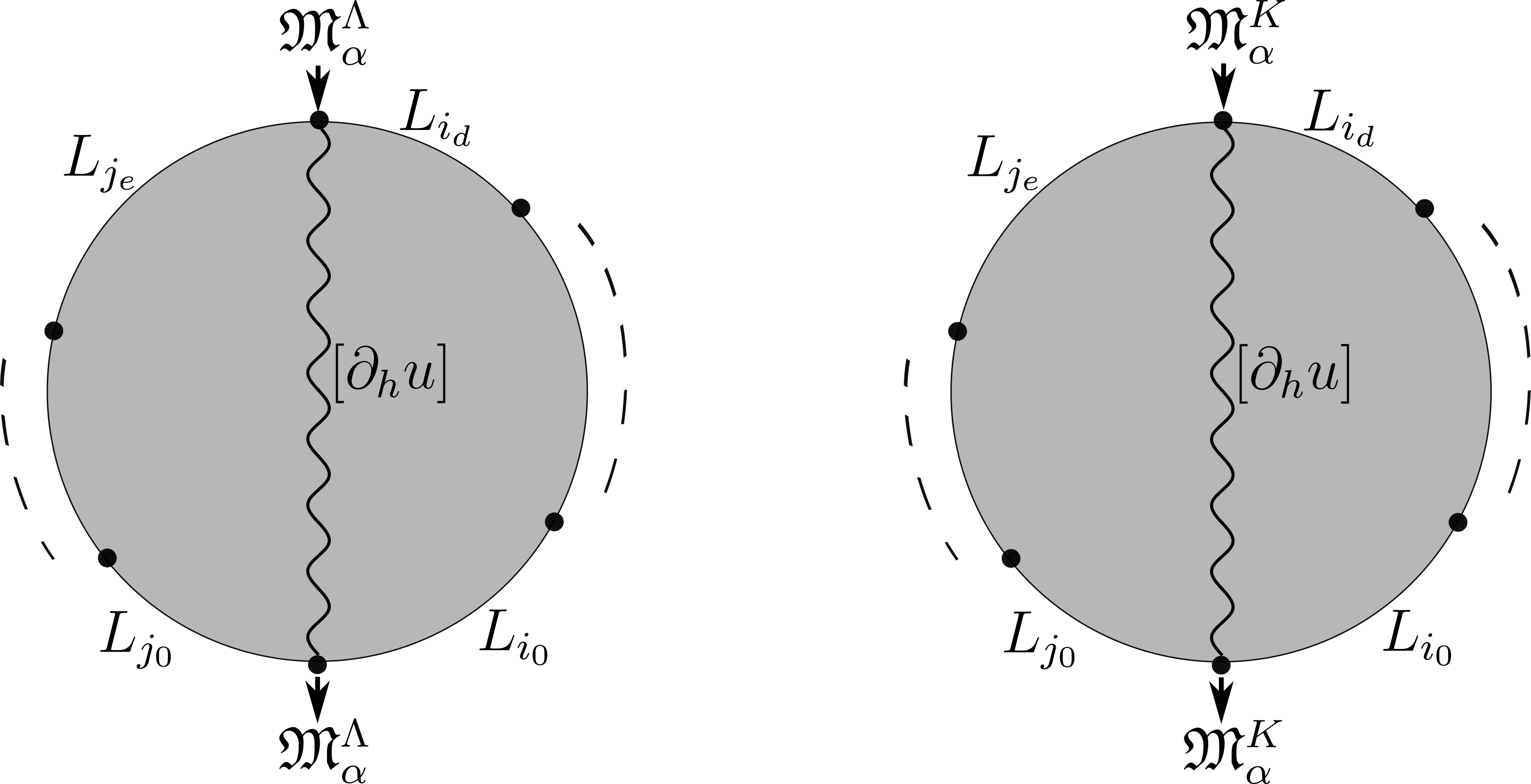
Figure 3.1. The counts defining $\mathfrak{M}_{\alpha}^{\Lambda}$ and $\mathfrak{M}^{K}_{\alpha}$

We use the term Novikov family for both $K$ and $\Lambda$. Which type of family we are working with will be clear from the notation.

For an additive subgroup $G\subset{\mathbb{R}}$ such that $T^{g}\in K$ for all $g\in G$, one can also consider the ring $K[z^{G}]$, sums of monomials $z^{g},g\in G$.

Definition 3.2.

We define the family $\mathfrak{M}_{\alpha}^{K}$ of ${\mathcal{F}}(M,K)$-bimodules via

(3.8) $$(L_{i},L_{j})\mapsto\mathfrak{M}^{K}_{\alpha}(L_{i},L_{j})=CF(L_{i},L_{j};K)\otimes_{K}K[z^{\mathbb{R}}]$$

where $CF(L_{i},L_{j};K)=K\langle L_{i}\cap L_{j}\rangle$. To define the differential, consider the pseudo-holomorphic strips with boundary on $L_{i}$ and $L_{j}$ defining the Floer differential. Recall that we chose a base point on $M$ and relative homotopy classes of paths from this point to generators of $CF(L_{i},L_{j};\Lambda)$. Concatenate the chosen path from the base point to the input chord of the strip, the $L_{i}$ side of the boundary and the reverse of the path from the base point to output. Denote this class by $[\partial_{h}u]$, where $u$ is the Floer strip. Then, define the differential for (3.8) via the formula

(3.9) $$\mu^{1}(x)=\sum\pm T^{E(u)}z^{\alpha([\partial_{h}u])}.y$$

where $x$ and $y$ are generators of $CF(L_{i},L_{j};\Lambda)$ and $u$ ranges over the Floer strips with given boundary conditions, with input $x$ and output $y$. We obtain the more general structure maps of the family of bimodules by deforming the structure maps for the diagonal bimodule. Namely, the structure maps for diagonal bimodule send $(x_{k},\dots,x_{1}|x|x_{1}^{\prime},\dots x_{l}^{\prime})$ to signed sum

(3.10) $$\sum\pm T^{E(u)}.y$$

where the sum ranges over the discs with input $x_{l}^{\prime}\dots x,\dots,x_{k}$ and with output $y$. We define the structure maps for the family $\mathfrak{M}_{\alpha}^{K}$ via the formula

(3.11) $$\sum\pm T^{E(u)}z^{\alpha([\partial_{h}u])}.y$$

where $[\partial_{h}u]$ denotes the class obtained by concatenating the chosen path from the base point to $x$, $u\circ\gamma$ where $\gamma$ is a path in the marked disc from the marked point corresponding to $x$ to marked point corresponding to $y$, and the reverse of the chosen path from the base point to $y$ (See Figure 3.1, $[\partial_{h}u]$ is obtained by concatenating the wavy line in the figure with paths to base point).

Definition 3.3.

Let $\mathfrak{M}_{\alpha}^{\Lambda}$ denote the $\Lambda[z^{\mathbb{R}}]$-linear Novikov family of ${\mathcal{F}}(M,\Lambda)$-bimodules that is obtained by replacing $K$ by $\Lambda$ in Definition 3.2. Equivalently, this family can be obtained by extension of the coefficients of $\mathfrak{M}^{K}_{\alpha}$ along the inclusion map $K\to\Lambda$.

Note 3.4.

Let $\tilde{L}$ and $\tilde{L}^{\prime}$ be two Lagrangians that satisfy the conditions on $L$ and $L^{\prime}$ in Assumption 1.2. As mentioned in Remark 2.13, one can abstractly extend the Fukaya category to include $\tilde{L}$ and $\tilde{L}^{\prime}$ and the bimodule $\mathfrak{M}^{K}_{\alpha}$ to $\widetilde{\mathfrak{M}^{K}_{\alpha}}$. However, this extension by abstract means, whereas the notation $\widetilde{\mathfrak{M}_{\alpha}^{K}}(\tilde{L},\tilde{L}^{\prime})$ suggests the same concrete definition as (3.8). Therefore, we will use the complex

(3.12) $$h_{\tilde{L}^{\prime}}\otimes_{{\mathcal{F}}(M,K)}\mathfrak{M}_{\alpha}^{K}\otimes_{{\mathcal{F}}(M,K)}h^{\tilde{L}}$$

instead, which is well-defined whenever the modules $h_{\tilde{L}^{\prime}}$ and $h^{\tilde{L}}$ are defined over ${\mathcal{F}}(M,K)$.

Define $\mathfrak{M}_{f\alpha}^{\Lambda}:=\mathfrak{M}_{\alpha}^{\Lambda}|_{z=T^{f}}$ and $\mathfrak{M}_{f\alpha}^{K}:=\mathfrak{M}_{\alpha}^{K}|_{z=T^{f}}$, i.e. the base change of the respective family under the map $\Lambda[z^{\mathbb{R}}]\to\Lambda$, resp. $K[z^{\mathbb{R}}]\to K$ that sends $z^{r}$ to $T^{fr}$. The latter makes sense only for $f\in G_{(p)}\subset{\mathbb{R}}$. These are bimodules over ${\mathcal{F}}(M,\Lambda)$, resp. ${\mathcal{F}}(M,K)$.

Later we will show $\mathfrak{M}_{-f\alpha}^{K}$, together with the left-module corresponding to $L$ and right module corresponding to $L^{\prime}$ can be used to recover the groups $HF(\phi^{f}_{\alpha}L,L^{\prime})$ for some $f$, via the formula

(3.13) $$HF(\phi^{f}_{\alpha}(L),L^{\prime})\cong H^{*}(h_{L^{\prime}}\otimes_{{\mathcal{F}}(M,K)}\mathfrak{M}_{-f\alpha}^{\Lambda}\otimes_{{\mathcal{F}}(M,K)}h^{L})\otimes_{K}\Lambda$$

where $h_{L^{\prime}}$ denotes the right Yoneda module corresponding to $L^{\prime}$ and $h^{L}$ denotes the left Yoneda module corresponding to $L$.

We also note:

Lemma 3.5.

For $f,f^{\prime}\in{\mathbb{R}}$ such that $|f|,|f^{\prime}|$ are small, $\mathfrak{M}_{(f+f^{\prime})\alpha}^{\Lambda}\simeq\mathfrak{M}_{f\alpha}^{\Lambda}\otimes_{{\mathcal{F}}(M,\Lambda)}\mathfrak{M}_{f^{\prime}\alpha}^{\Lambda}$. The same statement holds for $\Lambda$ replaced by $K$ if $f,f^{\prime}\in{\mathbb{Z}}_{(p)}$.

We will prove a $p$-adic version of this statement in Proposition 3.20. A similar semi-continuity argument works in this case too, only one has to consider small $f,f^{\prime}$ with respect to Archimedean absolute value. More precisely, one can write a map

(3.14) $$\mathfrak{M}_{f\alpha}^{\Lambda}\otimes_{{\mathcal{F}}(M,\Lambda)}\mathfrak{M}_{f^{\prime}\alpha}^{\Lambda}\to\mathfrak{M}_{(f+f^{\prime})\alpha}^{\Lambda}$$

varying continuously in $f$ and $f^{\prime}$ that is similar to (3.25) and that restrict to a quasi-isomorphism at $f=f^{\prime}=0$. The main addition to ideas involved in the proof of Proposition 3.20 are about more general semi-continuity statements of chain complexes over $\Lambda[z^{\mathbb{R}}]$ (or over the ring $\Lambda\{z^{\mathbb{R}}\}$). We give a sketchy proof of Lemma 3.5 in Appendix A.

Remark 3.6.

One can give another proof of this statement for $f,f^{\prime}\in{\mathbb{Z}}_{(p)}$ with small $p$-adic absolute value. See Corollary 3.24.

3.2. p-adic arcs in Floer homology

Let $p>2$ be a prime number. We start by constructing an embedding ${\mathbb{Q}}(T^{G})\hookrightarrow{\mathbb{Q}}_{p}$ such that elements of the form $T^{g}$ map to elements of $1+p{\mathbb{Z}}_{p}$. More precisely, fix an integral basis $g_{1},\dots,g_{k}$ of the group $G$. Let $\mu_{1},\dots,\mu_{k}\in{\mathbb{Z}}_{p}$ be algebraically independent over ${\mathbb{Q}}$. Define a map $g_{i}\mapsto 1+p\mu_{i}$ from ${\mathbb{Q}}(T^{G})\to{\mathbb{Q}}_{p}$. This is well defined since $T^{g_{i}}$ are algebraically independent. We will extend it to a map ${\mathbb{Q}}(T^{G_{(p)}})\to{\mathbb{Q}}_{p}$ using Definition 3.7. Recall that ${\mathbb{Q}}_{p}\langle t\rangle=\{\sum_{n}a_{n}t^{n}:n{\mathbb{N}},a_{n}\in{\mathbb{Q}}_{p},val_{p}(a_{n})\to\infty\}$ is the Tate algebra over ${\mathbb{Q}}_{p}$ with one variable, and it can be thought as the set of analytic functions on the $p$-adic unit disc ${\mathbb{Z}}_{p}$:

Definition 3.7.

[[BSS17]] Let $v=1+\nu\in 1+p{\mathbb{Z}}_{p}$. Define $v^{t}\in{\mathbb{Q}}_{p}\langle t\rangle$ to be the function

(3.15) $$(1+(v-1))^{t}=(1+\nu)^{t}:=\sum_{i=0}^{\infty}{t\choose i}\nu^{i}$$

The convergence of (3.15) on ${\mathbb{Z}}_{p}$ is clear, see also [BSS17, Proposition 2.1]. Let us list some properties, mainly following [BSS17]:

1. $v^{t}$ is the $n^{th}$ power of $v$ when $t=n\in{\mathbb{N}}$

2. $v^{t+t^{\prime}}=v^{t}v^{t^{\prime}}\in{\mathbb{Q}}_{p}\langle t,t^{\prime}\rangle$

3. $(v_{1}v_{2})^{t}=v_{1}^{t}v_{2}^{t}$

Proof.

(1) follows from the binomial theorem. To see (3), check it first on ${\mathbb{N}}\subset{\mathbb{Z}}_{p}$ using (1). A functional equation that holds on a dense (or just infinite) subset of ${\mathbb{Z}}_{p}$ holds over ${\mathbb{Q}}_{p}\langle t\rangle$ by Strassman’s theorem (see [Kat07, Theorem 3.38]).

Similarly, to see (2), check it first on ${\mathbb{N}}\times{\mathbb{N}}\subset{\mathbb{Z}}_{p}\times{\mathbb{Z}}_{p}$ using (1), and conclude by density that the equation holds on ${\mathbb{Z}}_{p}\times{\mathbb{Z}}_{p}$. By an iterated application of Strassman’s theorem, we obtain (2). ∎

We can define the map from $\mu:{\mathbb{Q}}(T^{G_{(p)}})\to{\mathbb{Q}}_{p}$ as the map satisfying

(3.16) $$T^{g_{i}/n}\mapsto(1+p\mu_{i})^{1/n}$$

where $p\nmid n$ and $1/n^{th}$ power is taken by specialization of $(1+p\mu_{i})^{t}$ to $t=1/n$. Therefore, the elements of type $T^{a}$ map to elements of $1+p{\mathbb{Z}}_{p}$. Since $\mu_{i}$ are algebraically independent, this gives a well-defined map ${\mathbb{Q}}(T^{G_{(p)}})\to{\mathbb{Q}}_{p}$. To see this, first notice ${\mathbb{Q}}[T^{G_{(p)}}]\to{\mathbb{Q}}_{p}$ is well-defined as the former is the group algebra. If an element of ${\mathbb{Q}}[T^{G_{(p)}}]$ maps to $0\in{\mathbb{Q}}_{p}$, this gives a non-trivial algebraic relation over ${\mathbb{Q}}$ of elements $(1+p\mu_{i})^{1/N}$ for some large $N$. This is impossible as it would imply an algebraic relation between $1+p\mu_{i}$. We will denote $\mu(T^{a})$ also by $T_{\mu}^{a}$, where $a\in G_{(p)}$.

This defines a map $K\to{\mathbb{Q}}_{p}$. Let ${\mathcal{F}}(M,{\mathbb{Q}}_{p})$ denote the category obtained by extending the coefficients of ${\mathcal{F}}(M,K)$ to ${\mathbb{Q}}_{p}$.

The following is the $p$-adic analogue of Definition 3.1:

Definition 3.8.

For a given smooth and proper $A_{\infty}$-category ${\mathcal{B}}$ over ${\mathbb{Q}}_{p}$, a $p$-adic family $\mathfrak{M}$ of bimodules over $\mathcal{B}$ is an assignment of a free (${\mathbb{Z}}/2{\mathbb{Z}}$)-graded ${\mathbb{Q}}_{p}\langle t\rangle$-module $\mathfrak{M}(L,L^{\prime})$ to every pair of objects together with ${\mathbb{Q}}_{p}\langle t\rangle$-linear structure maps

(3.17) $${\mathcal{B}}(L^{\prime}_{1},L^{\prime}_{0})\otimes\dots\mathcal{B}(L^{\prime}_{m},L^{\prime}_{m-1})\otimes\mathfrak{M}(L_{n},L_{m}^{\prime})\otimes\dots\mathcal{B}(L_{0},L_{1})$$

(3.18) $$\to\mathfrak{M}(L_{0},L_{0}^{\prime})[1-m-n]$$

satisfying the standard bimodule equations. A (pre)-morphism of two families $\mathfrak{M}$ and $\mathfrak{M}^{\prime}$ is a collection of ${\mathbb{Q}}_{p}\langle t\rangle$-linear maps

(3.19) $$f^{m|1|n}:{\mathcal{B}}(L^{\prime}_{1},L^{\prime}_{0})\otimes\dots\mathcal{B}(L^{\prime}_{m},L^{\prime}_{m-1})\otimes\mathfrak{M}(L_{n},L_{m}^{\prime})\otimes\dots\mathcal{B}(L_{0},L_{1})$$

(3.20) $$\to\mathfrak{M}^{\prime}(L_{0},L_{0}^{\prime})[-m-n]$$

As before, the category of $p$-adic families form a ${\mathbb{Q}}_{p}\langle t\rangle$-linear pre-triangulated dg category, where the differential and composition are given by standard formulas for bimodules, and a morphism of families means a closed pre-morphism. The cone of a morphism is defined as the cone of underlying map of bimodules, equipped with the natural ${\mathbb{Q}}_{p}\langle t\rangle$-linear structure.

Definition 3.8 easily generalizes to other non-Archimedean fields extending ${\mathbb{Q}}_{p}$ as well as to Tate algebra with several variables ${\mathbb{Q}}_{p}\langle t_{1},\dots t_{n}\rangle$. Let $\mathfrak{M}$ be a family and $q$ be a ${\mathbb{Q}}_{p}$-point of $Sp({\mathbb{Q}}_{p}\langle t\rangle)$, i.e. a continuous ring homomorphism ${\mathbb{Q}}_{p}\langle t\rangle\to{\mathbb{Q}}_{p}$. Note that these ring homomorphisms are in correspondence with elements of ${\mathbb{Z}}_{p}$. One can define the restriction $\mathfrak{M}|_{t=q}$ as $\mathfrak{M}\otimes_{{\mathbb{Q}}_{p}\langle t\rangle}{\mathbb{Q}}_{p}$. This is an $A_{\infty}$-bimodule over ${\mathcal{B}}$.

Example 3.9.

For any bimodule $M$ over ${\mathcal{B}}$, one can define a p-adic family by $\mathfrak{M}(L,L^{\prime})=M(L,L^{\prime})\otimes_{{\mathbb{Q}}_{p}}{{\mathbb{Q}}_{p}\langle t\rangle}$ with the structure maps obtained by base change. This type of family has the same restrictions at every point. In particular, one can let $M$ to be a Yoneda bimodule $h^{L}\boxtimes h_{L^{\prime}}$ (i.e. the exterior tensor product of left and right Yoneda modules, see [Gan12, (2.83),(2.84)] for its structure maps). We call such a family a constant family of Yoneda bimodules.

One can define convolution of two families. First, recall the convolution of bimodules over ${\mathcal{B}}$:

Definition 3.10.

Let $M_{1}$ and $M_{2}$ be two bimodules over ${\mathcal{B}}$. Then, $M_{1}\otimes_{\mathcal{B}}M_{2}$ is the bimodule defined by

(3.21) $$(L,L^{\prime})\longmapsto\bigoplus M_{1}(L_{k},L^{\prime})\otimes{\mathcal{B}}(L_{k-1},L_{k})\otimes\dots\otimes{\mathcal{B}}(L_{1},L_{2})\otimes M_{2}(L,L_{1})[k]$$

where the direct sum is over all ordered sets $(L_{1},\dots,L_{k})$ for all $k\in{\mathbb{Z}}_{\geq 0}$. The differential is given by

(3.22) $$(m_{1}\otimes b_{1}\otimes\dots\otimes b_{f}\otimes m_{2})\mapsto\sum\pm\mu_{M_{1}}(m_{1}\otimes b_{1}\otimes\dots)\otimes\dots\otimes m_{2}+$$

$$\sum\pm m_{1}\otimes\dots\otimes\mu_{M_{2}}(\dots\otimes m_{2})+\sum\pm m_{1}\otimes\dots\otimes\mu_{\mathcal{B}}(\dots)\otimes\dots\otimes m_{2}$$

and other structure maps are defined similarly.

Definition 3.11.

Given families $\mathfrak{M}_{1}$ and $\mathfrak{M}_{2}$ over $Sp({\mathbb{Q}}_{p}\langle t\rangle)$, one can endow $\mathfrak{M}_{1}\otimes_{\mathcal{B}}\mathfrak{M}_{2}$ with the structure of a family over ${\mathbb{Q}}_{p}\langle t_{1},t_{2}\rangle$. One obtains a family over $Sp({\mathbb{Q}}_{p}\langle t\rangle)$ via base change along the (co)diagonal map ${\mathbb{Q}}_{p}\langle t_{1},t_{2}\rangle\to{\mathbb{Q}}_{p}\langle t\rangle,t_{1},t_{2}\mapsto t$. We denote this family by $\mathfrak{M}_{1}\otimes^{rel}_{\mathcal{B}}\mathfrak{M}_{2}$.

One can also construct $\mathfrak{M}_{1}\otimes^{rel}_{\mathcal{B}}\mathfrak{M}_{2}$ by performing the construction in Definition 3.10 ${\mathbb{Q}}_{p}\langle t\rangle$-linearly. One can see $\mathfrak{M}_{1}\otimes^{rel}_{\mathcal{B}}\mathfrak{M}_{2}$ as the fiberwise convolution of two families, i.e. as the tensor product relative to base; hence, the notation.

Example 3.12.

Let $\mathfrak{M}_{1}$ and $\mathfrak{M}_{2}$ be two constant families associated to bimodules $M_{1}$ and $M_{2}$ over ${\mathcal{B}}$. Then, $\mathfrak{M}_{1}\otimes^{rel}_{\mathcal{B}}\mathfrak{M}_{2}$ is the constant family associated to $M_{1}\otimes_{\mathcal{B}}M_{2}$. In particular, if $M_{1}=h^{L_{1}}\boxtimes h_{L^{\prime}_{1}}$ and $M_{2}=h^{L_{2}}\boxtimes h_{L^{\prime}_{2}}$, then $\mathfrak{M}_{1}\otimes^{rel}_{\mathcal{B}}\mathfrak{M}_{2}$ is the constant family associated to ${\mathcal{B}}(L_{2},L_{1}^{\prime})\otimes(h^{L_{1}}\boxtimes h_{L^{\prime}_{2}})$.

By Morita theory, a family of bimodules can be thought as a family of endomorphisms of the category. Therefore, if the parameter space of the family is a group, one can study “actions of this group on the category”. Observe ${\mathbb{Q}}_{p}\langle t\rangle$ is the ring of functions of a group, and is itself a Hopf algebra over ${\mathbb{Q}}_{p}$ with comultiplication given by $\Delta:t\mapsto t\otimes 1+1\otimes t$ (the counit is given by $e:t\mapsto 0$ and the antipodal map is given by $t\mapsto-t$).

Let $\pi_{i}:{\mathbb{Q}}_{p}\langle t\rangle\to{\mathbb{Q}}_{p}\langle t_{1},t_{2}\rangle$ denote the map $t\mapsto t_{i}$ for $i=1,2$. Given $p$-adic family $\mathfrak{M}$, one can extend the coefficients along $\pi_{1}$, $\pi_{2}$ and $\Delta$ to define three $2$-parameter $p$-adic family of bimodules denoted by $\pi_{1}^{*}\mathfrak{M}$, $\pi_{2}^{*}\mathfrak{M}$ and $\Delta^{*}\mathfrak{M}$ (we identify ${\mathbb{Q}}_{p}\langle t_{1},t_{2}\rangle$ with a suitable completion of ${\mathbb{Q}}_{p}\langle t\rangle\otimes{\mathbb{Q}}_{p}\langle t\rangle$ such that $t\otimes 1=t_{1},1\otimes t=t_{2}$). Define:

Definition 3.13.

A $p$-adic family $\mathfrak{M}$ of bimodules over ${\mathcal{B}}$ is called group-like if $\Delta^{*}\mathfrak{M}\simeq\pi_{1}^{*}\mathfrak{M}\otimes^{rel}_{\mathcal{B}}\pi_{2}^{*}\mathfrak{M}$ and if the restriction to counit $\mathfrak{M}|_{t=e}$ is quasi-isomorphic to diagonal bimodule.

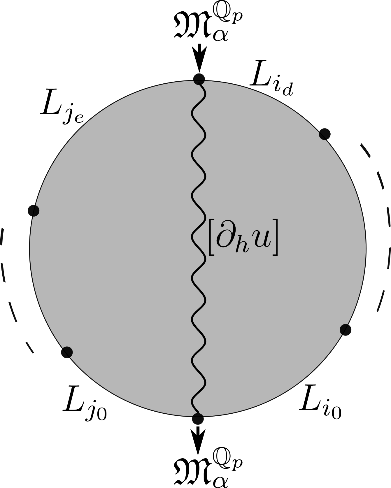
Figure 3.2. The counts defining $\mathfrak{M}_{\alpha}^{{\mathbb{Q}}_{p}}$

Clearly, if $\mathfrak{M}$ is group-like, and $f_{1},f_{2}\in{\mathbb{Z}}_{p}$, then $\mathfrak{M}|_{t=f_{1}+f_{2}}\simeq\mathfrak{M}|_{t=f_{1}}\otimes_{\mathcal{B}}\mathfrak{M}|_{t=f_{2}}$.

We want to construct an explicit group-like $p$-adic family $\mathfrak{M}_{\alpha}^{{\mathbb{Q}}_{p}}$ of bimodules over ${\mathcal{F}}(M,{\mathbb{Q}}_{p})$. To this end, associate

(3.23) $$(L_{i},L_{j})\mapsto\mathfrak{M}_{\alpha}^{{\mathbb{Q}}_{p}}(L_{i},L_{j})=CF(L_{i},L_{j};{\mathbb{Q}}_{p})\otimes{\mathbb{Q}}_{p}\langle t\rangle$$

The structure maps are defined via the formula

(3.24) $$(x_{1},\dots,x_{k}|x|x_{1}^{\prime},\dots,x_{l}^{\prime})\mapsto\sum\pm T_{\mu}^{E(u)}T_{\mu}^{t\alpha([\partial_{h}u])}.y$$

where the sum ranges over the marked discs with input $x_{l}^{\prime}\dots,x,x_{k},\dots,x_{1}$ and output $y$. The class $[\partial_{h}u]\in H_{1}(M;{\mathbb{Z}})$ is defined as before, and $\alpha([\partial_{h}u])\in G$ by definition of $G$; therefore, $T_{\mu}^{\alpha([\partial_{h}u])}=\mu(T^{\alpha([\partial_{h}u])})\in 1+p{\mathbb{Z}}_{p}$ is defined. Let $T_{\mu}^{t\alpha([\partial_{h}u])}\in{\mathbb{Q}}_{p}\langle t\rangle$ be its “$t^{th}$ power” as in Definition 3.7. The sum is finite and it is easy to check the bimodule equation is satisfied (see Figure 3.3 for instance). It is immediate that the restriction to $t=0$ is isomorphic to diagonal bimodule of ${\mathcal{F}}(M,{\mathbb{Q}}_{p})$. See also Figure 3.2.

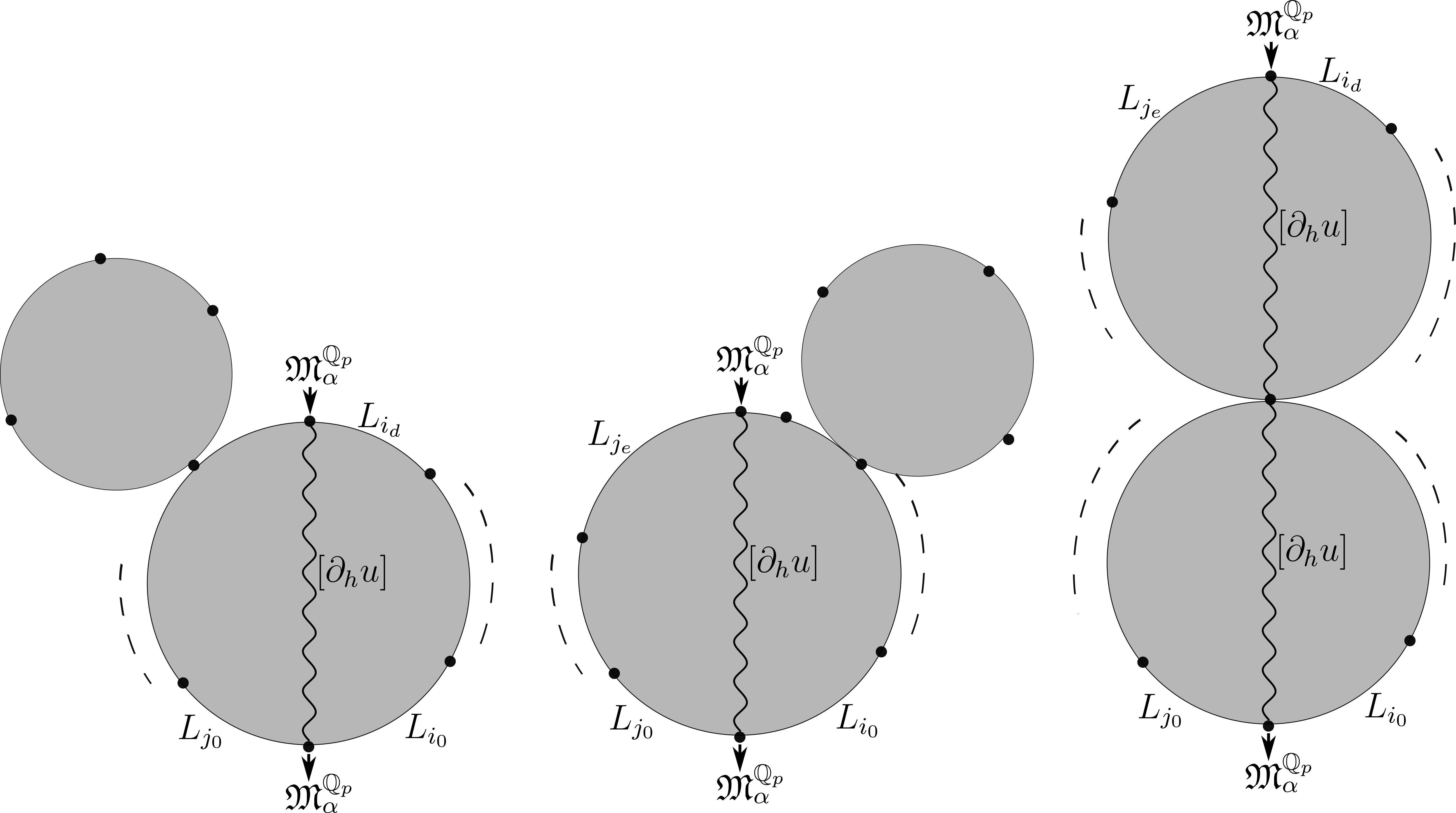
Figure 3.3. Some degenerations of discs as in Figure 3.2

To prove that this family is group-like, our next task to write a closed morphism of families

(3.25) $$\pi_{1}^{*}\mathfrak{M}_{\alpha}^{{\mathbb{Q}}_{p}}\otimes^{rel}_{{\mathcal{F}}(M,{\mathbb{Q}}_{p})}\pi_{2}^{*}\mathfrak{M}_{\alpha}^{{\mathbb{Q}}_{p}}\to\Delta^{*}\mathfrak{M}_{\alpha}^{{\mathbb{Q}}_{p}}$$

such that the restriction of (3.25) to $t_{1}=t_{2}=0$ to the quasi-isomorphism ${\mathcal{F}}(M,{\mathbb{Q}}_{p})\otimes_{{\mathcal{F}}(M,{\mathbb{Q}}_{p})}{\mathcal{F}}(M,{\mathbb{Q}}_{p})\to{\mathcal{F}}(M,{\mathbb{Q}}_{p})$ from the convolution of diagonal bimodule with itself to diagonal bimodule.

Given an $A_{\infty}$-category ${\mathcal{B}}$, it is a general result that ${\mathcal{B}}\otimes_{{\mathcal{B}}}{\mathcal{B}}\simeq{\mathcal{B}}$. Moreover, the bimodule quasi-isomorphism from left hand side to the right is given by

(3.26) $$g^{k|1|l}:(x_{1},\dots,x_{k}|x\otimes b_{1}\otimes\dots\otimes b_{f}\otimes x^{\prime}|x_{1}^{\prime},\dots x_{l}^{\prime})\mapsto\atop\pm\mu_{\mathcal{B}}(x_{1},\dots,x_{k},x,b_{1},\dots b_{f},x^{\prime},x_{1}^{\prime},\dots x_{l}^{\prime})$$

Here, $x\otimes b_{1}\otimes\dots\otimes b_{f}\otimes x^{\prime}$ is the element of ${\mathcal{B}}\otimes_{\mathcal{B}}{\mathcal{B}}$. When ${\mathcal{B}}$ is the Fukaya category, this map is geometrically given by the count of marked discs as usual. To deform it, we define the following cohomology classes: given a pseudo-holomorphic disc $u$ with output $y$ and with input given by generators $x_{1},\dots,x_{k}$, $x$, $b_{1}\dots,b_{f}$, $x^{\prime}$, $x_{1}^{\prime},\dots x_{l}^{\prime}$ (in counter-clockwise direction after output), define $[\partial_{1}\alpha]\in H_{1}(M;{\mathbb{Z}})$ to be the path obtained by concatenating the fixed path from the base point of $M$ to generator $x$, the image under $u$ of a path from the input marked point for $x$ to output marked point, and the reverse of the path from the base point to $y$. We think of this class as the portion of boundary of $u$ from $x$ to $y$. Similarly define $[\partial_{2}u]\in H_{1}(M;{\mathbb{Z}})$ by replacing $x$ with $x^{\prime}$. The class $[\partial_{2}u]$ can be thought as the portion of boundary from $x^{\prime}$ to $y$. In other words, the paths $[\partial_{1}u]$ and $[\partial_{2}u]$ are obtained by concatenating the $u$-image of the respective wavy line in Figure 3.4 with chosen paths from the base point to the generator. To define the map (3.25), fix input $x_{1},\dots,x_{k},x,b_{1}\dots,b_{f},x^{\prime},x_{1}^{\prime},\dots x_{l}^{\prime}$ as above. The coefficient of $y$ under the map (3.25) is given by

(3.27) $$\sum\pm T_{\mu}^{E(u)}T_{\mu}^{t_{1}\alpha([\partial_{1}u])}T_{\mu}^{t_{2}\alpha([\partial_{2}u])}.y$$

where $u$ range over the pseudo-holomorphic discs with given input and output. See Figure 3.4. The input $x$, resp. $x^{\prime}$ is associated to marked point labeled as $\pi_{1}^{*}\mathfrak{M}_{\alpha}^{{\mathbb{Q}}_{p}}$, resp. $\pi_{2}^{*}\mathfrak{M}_{\alpha}^{{\mathbb{Q}}_{p}}$, and the output $y$ is associated to $\Delta^{*}\mathfrak{M}_{\alpha}^{{\mathbb{Q}}_{p}}$.

Recall that $T_{\mu}^{\alpha([\partial_{1}u])}:=\mu(T^{\alpha([\partial_{1}u])})\in 1+p{\mathbb{Z}}_{p}$. As before $T_{\mu}^{t_{1}\alpha([\partial_{1}u])}\in{\mathbb{Q}}_{p}\langle t_{1}\rangle\subset{\mathbb{Q}}_{p}\langle t_{1},t_{2}\rangle$ is its $t_{1}^{th}$-power as in Definition 3.7. $T_{\mu}^{t_{2}\alpha([\partial_{2}u])}$ is defined similarly. It is easy to check this defines a map of bimodules (3.25). See for instance Figure 3.5. Moreover, it restricts to the standard quasi-isomorphism of diagonal bimodules at $t_{1}=t_{2}=0$ defined by (3.26).

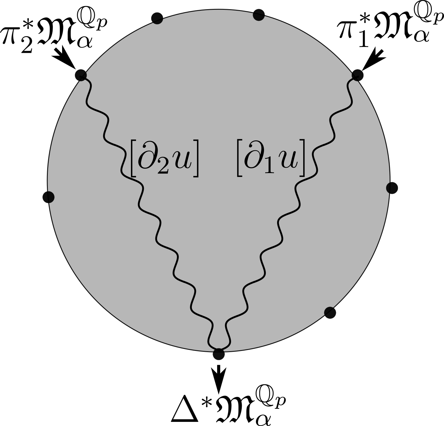
Figure 3.4. The counts defining (3.25)

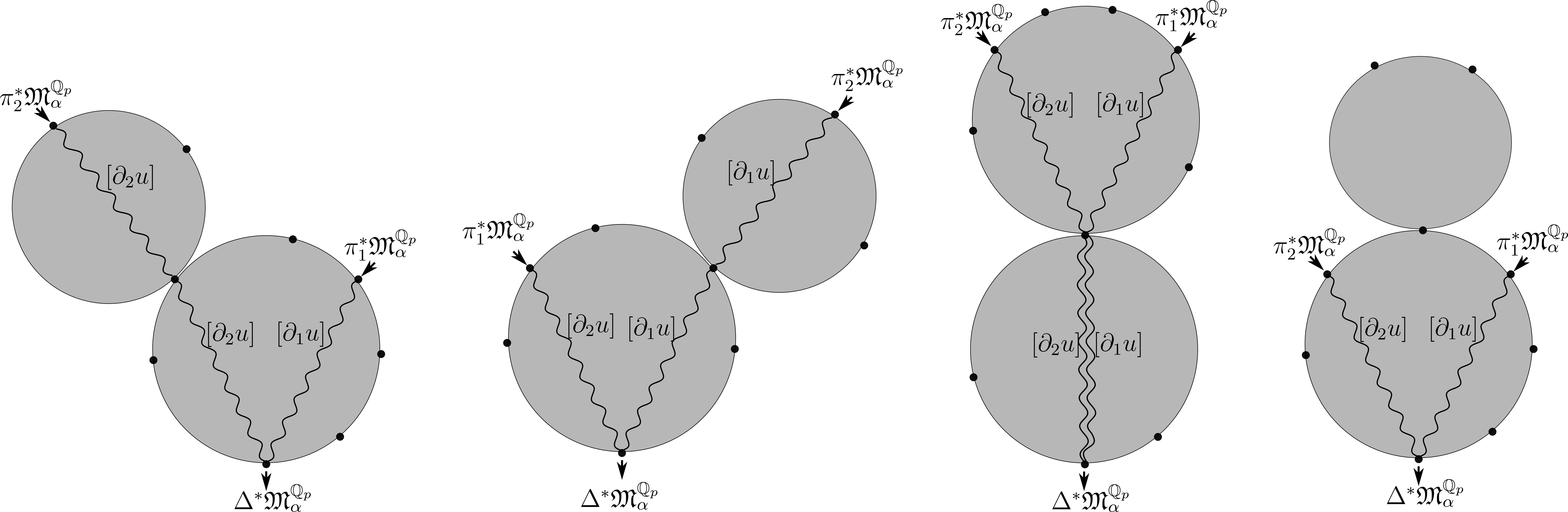
Figure 3.5. Some degenerations of moduli of discs as in Figure 3.4

Our next task is to prove (3.25) is a quasi-isomorphism. This relies on a semi-continuity argument for which we need a properness result for the domain of (3.25), i.e. we need to show that this family is a cohomologically finitely generated ${\mathbb{Q}}_{p}\langle t\rangle$-module at every pair of objects $(L,L^{\prime})$. We need some technical preparation for this:

Definition 3.14.

A family $\mathfrak{M}$ is called perfect if it is quasi-isomorphic to a direct summand of a twisted complex of constant families of Yoneda bimodules in the category of families. It is called locally perfect if there is an admissible cover of $Sp({\mathbb{Q}}_{p}\langle t\rangle)$ (or any other parameter space we are using) such that each restriction of $\mathfrak{M}$ is perfect. $\mathfrak{M}$ is called proper if the cohomology of $\mathfrak{M}(L,L^{\prime})$ is finitely generated over ${\mathbb{Q}}_{p}\langle t\rangle$ for all $L,L^{\prime}$.

Clearly, perfect implies locally perfect and if ${\mathcal{B}}$ is a proper category, locally perfect implies proper. We will see that proper implies perfect for a smooth, proper $A_{\infty}$-category ${\mathcal{B}}$. For simplicity, we start with the following:

Lemma 3.15.

Let ${\mathcal{B}}$ be a smooth and proper $A_{\infty}$-category over a field of characteristic $0$. A proper right/left-module or a bimodule over ${\mathcal{B}}$ is perfect.

Proof.

Let $M$ be a proper right module over ${\mathcal{B}}$. Then, $M\otimes_{\mathcal{B}}{\mathcal{B}}\simeq M$ as right modules. One can represent the diagonal bimodule ${\mathcal{B}}$ in terms of Yoneda bimodules $h^{L}\boxtimes h_{L^{\prime}}$, where $h^{L}$ denote the left Yoneda module, $h_{L^{\prime}}$ denote the right Yoneda module, and $\boxtimes$ is for exterior tensor product (see [Gan12, (2.83),(2.84)]). Observe

(3.28) $$M\otimes_{\mathcal{B}}(h^{L}\boxtimes h_{L^{\prime}})\simeq M(L)\otimes h_{L^{\prime}}$$

Therefore, $M$ can be written as direct a summand of a twisted complex (iterated cone) of modules of type $M(L)\otimes_{{\mathcal{B}}}h_{L^{\prime}}$, but the latter is quasi-isomorphic to finitely many copies of $h_{L^{\prime}}$ as $M$ is proper. This concludes the proof.

The proof is the same for left modules, and for bimodules one uses

(3.29) $$M\simeq{\mathcal{B}}\otimes_{{\mathcal{B}}}M\otimes_{{\mathcal{B}}}{\mathcal{B}}$$

together with the finite resolution of the diagonal on both sides. ∎

Assume ${\mathcal{B}}$ is smooth and proper $A_{\infty}$-category over ${\mathbb{Q}}_{p}$ (or over a subfield of ${\mathbb{Q}}_{p}$). Lemma 3.15 immediately generalizes to:

Lemma 3.16.

A proper $p$-adic family of bimodules over ${\mathcal{B}}$ is perfect.

Proof.

Let $\mathfrak{M}$ be a proper family. The quasi-isomorphism

(3.30) $$\mathfrak{M}\simeq{\mathcal{B}}\otimes_{{\mathcal{B}}}\mathfrak{M}\otimes_{{\mathcal{B}}}{\mathcal{B}}$$

still holds true, and by using the representation of the diagonal bimodule as a direct summand of twisted complex of Yoneda bimodules, we see that $\mathfrak{M}$ is quasi-isomorphic to a direct summand of a twisted complex of families of the form

(3.31) $$(h^{L_{1}}\boxtimes h_{L_{1}^{\prime}})\otimes_{{\mathcal{B}}}\mathfrak{M}\otimes_{{\mathcal{B}}}(h^{L_{2}}\boxtimes h_{L_{2}^{\prime}})\simeq\mathfrak{M}(L_{2},L_{1}^{\prime})\otimes(h^{L_{1}}\boxtimes h_{L_{2}^{\prime}})$$

Therefore, it suffices to show the last type of family is perfect. Note that here we consider $\mathfrak{M}(L_{2},L_{1}^{\prime})$ as a chain complex over ${\mathbb{Q}}_{p}\langle t\rangle$, and $(h^{L_{1}}\boxtimes h_{L_{2}^{\prime}})$ is the Yoneda bimodule as before. The family structure on their tensor product is obvious.

By assumption, $\mathfrak{M}(L_{2},L_{1}^{\prime})$ has finitely generated cohomology over ${\mathbb{Q}}_{p}\langle t\rangle$ (or whichever parameter space we are using). By [Ked04, Proposition 6.5], every finitely generated module over the affinoid domain has a finite free resolution, and this immediately implies the existence of finitely generated free complex $C$ of modules over the affinoid domain quasi-isomorphic to $\mathfrak{M}(L_{2},L_{1}^{\prime})$. It is easy to see that

(3.32) $$C\otimes(h^{L_{1}}\boxtimes h_{L_{2}^{\prime}})\simeq\mathfrak{M}(L_{2},L_{1}^{\prime})\otimes(h^{L_{1}}\boxtimes h_{L_{2}^{\prime}})$$

is perfect. This completes the proof. ∎

Remark 3.17.

The notions of $p$-adic family of left/right modules can be defined similarly. Then, Lemma 3.16 still holds for such families.

Corollary 3.18.

Let $\mathfrak{M}_{1}$ and $\mathfrak{M}_{2}$ be two proper $p$-adic families (over an affinoid domain as before). Then the convolution $\mathfrak{M}_{1}\otimes^{rel}_{{\mathcal{B}}}\mathfrak{M}_{2}$ is proper.

Proof.

By Lemma 3.16, both families are perfect; therefore, they can be represented as summands of complexes of constant families of Yoneda bimodules. It follows from Example 3.12 that the convolution of two constant families of Yoneda bimodules is perfect; hence, proper. Therefore, $\mathfrak{M}_{1}\otimes^{rel}_{{\mathcal{B}}}\mathfrak{M}_{2}$ can be represented as the direct summand of a twisted complex (iterated cone) of proper modules and it is proper itself. ∎

Corollary 3.19.

Let $\mathfrak{N}$ denote the cone of the morphism (3.25). Then, $H^{*}(\mathfrak{N}(L_{i},L_{j}))$ is a finitely generated module over ${\mathbb{Q}}_{p}\langle t_{1},t_{2}\rangle$ for all $L_{i},L_{j}$, i.e. $\mathfrak{N}$ is proper.

Proof.

By construction, $\pi_{1}^{*}\mathfrak{M}_{\alpha}^{{\mathbb{Q}}_{p}}$ and $\pi_{2}^{*}\mathfrak{M}_{\alpha}^{{\mathbb{Q}}_{p}}$ are both proper modules; therefore, by Corollary 3.18, $\pi_{1}^{*}\mathfrak{M}_{\alpha}^{{\mathbb{Q}}_{p}}\otimes^{rel}_{{\mathcal{F}}(M,{\mathbb{Q}}_{p})}\pi_{2}^{*}\mathfrak{M}_{\alpha}^{{\mathbb{Q}}_{p}}$ is also proper. Since $\Delta^{*}\mathfrak{M}_{\alpha}^{{\mathbb{Q}}_{p}}$ is proper too, the cone of a morphism

(3.33) $$\pi_{1}^{*}\mathfrak{M}_{\alpha}^{{\mathbb{Q}}_{p}}\otimes^{rel}_{{\mathcal{F}}(M,{\mathbb{Q}}_{p})}\pi_{2}^{*}\mathfrak{M}_{\alpha}^{{\mathbb{Q}}_{p}}\to\Delta^{*}\mathfrak{M}_{\alpha}^{{\mathbb{Q}}_{p}}$$

is proper. This completes the proof. ∎

Proposition 3.20.

$H^{*}(\mathfrak{N})$ vanishes on the smaller affinoid domain ${\mathbb{Q}}_{p}\langle t_{1}/p^{n},t_{2}/p^{n}\rangle$ for a sufficiently large $n$. Therefore, $\mathfrak{M}_{\alpha}^{{\mathbb{Q}}_{p}}|_{{\mathbb{Q}}_{p}\langle t/p^{n}\rangle}$ is group-like.

Proof.

By Lemma 3.19, the cohomology of $\mathfrak{N}$ is finitely generated over ${\mathbb{Q}}_{p}\langle t_{1},t_{2}\rangle$, and it vanishes at $t_{1}=t_{2}=0$ (as (3.25) is a quasi-isomorphism at $t_{1}=t_{2}=0$). As in the proof of Lemma 3.16, [Ked04, Proposition 6.5] implies that each $\mathfrak{N}(L_{i},L_{j})$ is quasi-isomorphic to a free finite complex of ${\mathbb{Q}}_{p}\langle t_{1},t_{2}\rangle$-modules. Then, the result follows from the following standard result, applied to a free finite complex quasi-isomorphic to $\bigoplus_{i,j}\mathfrak{N}(L_{i},L_{j})$. ∎

Lemma 3.21.

Let $(C,d)$ be a free, finite complex of ${\mathbb{Q}}_{p}\langle t_{1},t_{2}\rangle$ modules whose restriction to $t_{1}=t_{2}=0$ is acyclic. Then, for sufficiently large $n$, the restriction of $(C,d)$ to ${\mathbb{Q}}_{p}\langle t_{1}/p^{n},t_{2}/p^{n}\rangle$ is acyclic.

Proof.

By choosing a trivialization of the graded module $C$, one can see $d$ as a square matrix of elements of ${\mathbb{Q}}_{p}\langle t_{1},t_{2}\rangle$. The rank of $H^{*}(C,d)$ at a point $(p_{1},p_{2})$ is the same as

(3.34) $$rank(C)-2rank(d|_{t_{1}=p_{1},t_{2}=p_{2}})$$

The rank of $d$ is maximal and is equal to $rank(C)/2$ at $t_{1}=t_{2}=0$, and there is a square submatrix of $d$ of size $rank(C)/2$, whose determinant is non-vanishing at $t_{1}=t_{2}=0$. Let $f(t_{1},t_{2})\in{\mathbb{Q}}_{p}\langle t_{1},t_{2}\rangle$ denote the determinant of this submatrix, normalized by a constant so that $f(0,0)=1$.

As $f(0,0)=1$, $f$ has an inverse defined on a formal neighborhood of $(0,0)$, and this inverse converges over points of sufficiently large valuation. More precisely, let $f(t_{1},t_{2})=1+\sum a_{k,l}t_{1}^{k}t_{2}^{l}$, where $a_{k,l}\in{\mathbb{Q}}_{p}$. Then $val_{p}a_{k,l}\to\infty$ as $f$ converges over ${\mathbb{Z}}_{p}\times{\mathbb{Z}}_{p}$. Therefore, all but finitely many of $a_{k,l}$ are $O(p)$, i.e. $a_{k,l}\in p{\mathbb{Z}}_{p}$. By choosing $n$ large enough, we can ensure other terms except the constant term are also $O(p)$; hence, $f$ takes non-zero values over $p^{n}{\mathbb{Z}}_{p}\times p^{n}{\mathbb{Z}}_{p}$ and its inverse converge over this set. In other words, $f$ is invertible in the ring ${\mathbb{Q}}_{p}\langle t_{1}/p^{n},t_{2}/p^{n}\rangle$.

This implies that for any ring homomorphism ${\mathbb{Q}}_{p}\langle t_{1}/p^{n},t_{2}/p^{n}\rangle\to Q$ to a field, the rank of $H^{*}(C\otimes Q,d\otimes 1_{Q})$ is $0$, i.e. $H^{*}(C\otimes Q,d\otimes 1_{Q})$ vanishes. Then, given curve $S\subset Sp({\mathbb{Q}}_{p}\langle t_{1}/p^{n},t_{2}/p^{n}\rangle)$ and a ring homomorphism ${\mathcal{O}}^{an}(S)\to Q$ to a field we have a spectral sequence with $E_{2}$-page

(3.35) $$Tor_{p}(H^{-q}(C|_{{\mathcal{O}}^{an}(S)},d|_{{\mathcal{O}}^{an}(S)}),Q)\Rightarrow H^{-p-q}(C\otimes Q,d\otimes 1)=0$$

where the $Tor$ is also over ${{\mathcal{O}}^{an}(S)}$, and it is supported at $p=0,1$ as $S$ is a curve. Therefore, this spectral sequence degenerates at $E_{2}$-page. Hence, $H^{-q}(C|_{{\mathcal{O}}^{an}(S)},d|_{{\mathcal{O}}^{an}(S)})\otimes Q=0$, for all such $Q$, which implies $H^{-q}(C|_{{\mathcal{O}}^{an}(S)},d|_{{\mathcal{O}}^{an}(S)})=0$.This holds for any curve $S$. Likewise, consider the spectral sequence

(3.36) $$Tor_{p}(H^{-q}(C,d),{\mathcal{O}}^{an}(S))\Rightarrow H^{-p-q}(C|_{{\mathcal{O}}^{an}(S)},d|_{{\mathcal{O}}^{an}(S)})=0$$

This time, $Tor$ is over ${\mathbb{Q}}_{p}\langle t_{1}/p^{n},t_{2}/p^{n}\rangle$, and $Tor_{p}(\cdot,{\mathcal{O}}^{an}(S))$ is supported at $p=0,1$ as $S$ is of codimension $1$. As before, this lets us conclude $H^{-q}(C,d)\otimes{\mathcal{O}}^{an}(S)$ for all such $S$, and this implies $H^{*}(C|_{{\mathbb{Q}}_{p}\langle t_{1}/p^{n},t_{2}/p^{n}\rangle},d|_{{\mathbb{Q}}_{p}\langle t_{1}/p^{n},t_{2}/p^{n}\rangle})=0$, finishing the proof.∎

Remark 3.22.

It is easy to see that $\mathbb{Q}_{p}\langle t/p^{n}\rangle$ is the set of power series in $t$ that converge over $p^{n}{\mathbb{Z}}_{p}$. Therefore, the Berkovich spectrum $Sp(\mathbb{Q}_{p}\langle t/p^{n}\rangle)$ is actually a smaller subdomain inside $Sp(\mathbb{Q}_{p}\langle t\rangle)$; however, contrary to Archimedean geometry, it is also a subgroup. In particular, the iterates of this “neighborhood of $(0,0)$” does not cover ${\mathbb{Q}}_{p}\langle t\rangle$.

Remark 3.23.

Presumably, using the machinery of deformation classes of [Sei14], one can show that the family $\mathfrak{M}_{\alpha}^{{\mathbb{Q}}_{p}}$ is already group-like without restricting to $Sp(\mathbb{Q}_{p}\langle t/p^{n}\rangle)$.

Even though Proposition 3.20 is about the family ${\mathbb{Q}}_{p}$, it still allows us to conclude a weak group-like statement for the family $\mathfrak{M}_{\alpha}^{\Lambda}$. Recall the notation $\mathfrak{M}_{f\alpha}^{K}:=\mathfrak{M}_{\alpha}^{K}|_{z=T^{f}}$, for $f\in{\mathbb{R}}$.

Corollary 3.24.

Let $f,f^{\prime}\in p^{n}{\mathbb{Z}}_{(p)}\subset{\mathbb{Q}}$. Then, $\mathfrak{M}^{K}_{f\alpha}\otimes_{{\mathcal{F}}(M,K)}\mathfrak{M}^{K}_{f^{\prime}\alpha}\simeq\mathfrak{M}^{K}_{(f+f^{\prime})\alpha}$. The same statement holds if $K$ is replaced by $\Lambda$.

Proof.

One can define the map

(3.37) $$\mathfrak{M}^{K}_{f\alpha}\otimes_{{\mathcal{F}}(M,K)}\mathfrak{M}^{K}_{f^{\prime}\alpha}\to\mathfrak{M}^{K}_{(f+f^{\prime})\alpha}$$

similar to (3.25). More precisely, one would need to replace (3.27) by

(3.38) $$\sum\pm T^{E(u)}T^{f\alpha\cdot[\partial_{1}u]}T^{f^{\prime}\alpha\cdot[\partial_{2}u]}.y$$

and it is easy to check this defines a bimodule map. Moreover, after the base change along $\mu:K\to{\mathbb{Q}}_{p}$, the map (3.37) becomes same as (3.27) evaluated at $t_{1}=f,t_{2}=f^{\prime}$ considered as elements of $p^{n}{\mathbb{Z}}_{p}\subset{\mathbb{Q}}_{p}$. Same holds for the cone of (3.37). By Proposition 3.20, this cone vanishes after base-change, implying it is $0$ before the base change as well. Therefore, (3.37) is a quasi-isomorphism before the base change as well. One can then apply base change along the inclusion $K\to\Lambda$ to conclude $\mathfrak{M}^{\Lambda}_{f\alpha}\otimes_{{\mathcal{F}}(M,\Lambda)}\mathfrak{M}^{\Lambda}_{f^{\prime}\alpha}\simeq\mathfrak{M}^{\Lambda}_{(f+f^{\prime})\alpha}$. ∎

4. Comparison with the action of $\phi^{t}_{\alpha}$ and proof of Theorem 1.1

We need the following proposition to conclude the proof of Theorem 1.1:

Proposition 4.1.

For any $f\in p^{n}{\mathbb{Z}}_{(p)}$,

(4.1) $$HF(\phi^{f}_{\alpha}(L),L^{\prime})\cong HF(L,\phi^{-f}_{\alpha}(L^{\prime}))\cong H^{*}(\mathfrak{M}^{\Lambda}_{\alpha}|_{z=T^{-f}}(L,L^{\prime}))$$

and this group has the same dimension over $\Lambda$ as

(4.2) $$dim_{K}\big{(}H^{*}\big{(}h_{L^{\prime}}\otimes_{{\mathcal{F}}(M,K)}\mathfrak{M}^{K}_{\alpha}|_{z=T^{-f}}\otimes_{{\mathcal{F}}(M,K)}h^{L}\big{)}\big{)}=\atop dim_{{\mathbb{Q}}_{p}}\big{(}H^{*}\big{(}h_{L^{\prime}}\otimes_{{\mathcal{F}}(M,{\mathbb{Q}}_{p})}\mathfrak{M}^{{\mathbb{Q}}_{p}}_{\alpha}|_{t=-f}\otimes_{{\mathcal{F}}(M,{\mathbb{Q}}_{p})}h^{L}\big{)}\big{)}$$

As before, we denote $\mathfrak{M}_{\alpha}^{\Lambda}|_{z=T^{f}}$ by $\mathfrak{M}_{f\alpha}^{\Lambda}$ as well. We want to show the bimodules $\mathfrak{M}_{f\alpha}^{\Lambda}$ act on the perfect modules coming from Lagrangians in the expected way.

Recall that for a given $\tilde{L}\subset M$ satisfying some assumptions (such as $\tilde{L}\pitchfork L_{i}$ for all $i$), we have a right ${\mathcal{F}}(M,\Lambda)$-module $h_{\tilde{L}}$ that satisfies $h_{\tilde{L}}(L_{i})=CF(L_{i},\tilde{L})=CF(L_{i},\tilde{L};\Lambda)$. The differential and structure maps are defined by counting marked discs with one boundary component on $\tilde{L}$, and with other boundary components on various $L_{i}$. We will deform this module algebraically to give a simpler description of $h_{\phi_{\alpha}^{f}(\tilde{L})}$ for small $f$:

Definition 4.2.

Fix homotopy classes of paths from the base point of $M$ to intersection points $\tilde{L}\cap L_{i}$. Let $h_{\phi_{\alpha}^{f},\tilde{L}}^{alg}$ denote the right ${\mathcal{F}}(M,\Lambda)$-module defined by

(4.3) $$L_{i}\mapsto CF(L_{i},\tilde{L})$$

and whose differential/structure maps are given by

(4.4) $$\sum\pm T^{E(u)}T^{f\alpha([\partial_{2}u])}.y$$

where $u$ range over holomorphic curves with one boundary component on $\tilde{L}$ (the one on the clockwise direction from the output) and other components on $L_{i}$. Here, $y$ is the output marked point and $[\partial_{2}u]\in H_{1}(M;{\mathbb{Z}})$ denote the homology class of the path obtained by concatenating the fixed paths from the base point with ($u$-image of) the wavy path in Figure 4.1 from the module input to module output $y$ (this is very related to class previously denoted by $[\partial_{2}u]$, and we use the same notation as no confusion can arise).

Clearly, $h_{\phi_{\alpha}^{0},\tilde{L}}^{alg}=h_{\tilde{L}}$; therefore, one can see $h_{\phi_{\alpha}^{f},\tilde{L}}^{alg}$ as a deformation of $h_{\tilde{L}}$. The proof of the following Lemma implies (4.4) converge $T$-adically, i.e. $h_{\phi_{\alpha}^{f},\tilde{L}}^{alg}$ is well-defined, for small $|f|$:

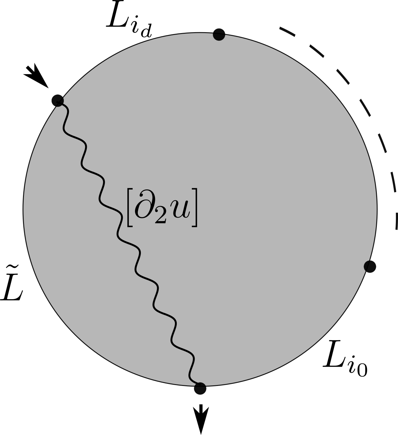
Figure 4.1. The counts defining $h^{alg}_{\phi_{\alpha}^{f},\tilde{L}}$, which gives a simpler quasi-isomorphic description of $h_{\phi^{f}_{\alpha}(\tilde{L})}$

Lemma 4.3.

For $f\in{\mathbb{R}}$ such that $|f|$ is small, we have $h_{\phi_{\alpha}^{f},\tilde{L}}^{alg}\simeq h_{\phi_{\alpha}^{f}(\tilde{L})}$. In other words, $h_{\phi_{\alpha}^{f},\tilde{L}}^{alg}$ gives what is expected geometrically.

Proof.

This is an application of Fukaya’s trick, see [Abo14], for instance. Namely, if $f$ is small enough, the intersection points $\phi^{f}_{\alpha}(\tilde{L})\cap L_{i}$ can be identified with $\tilde{L}\cap L_{i}$, and this holds throughout the isotopy. Consider a smooth isotopy $\psi^{f}$ of $M$ fixing all $L_{i}$ setwise and mapping $\tilde{L}$ to $\phi^{f}_{\alpha}(\tilde{L})$. Choose the almost complex structures for $(L_{i},\tilde{L})$ and $(L_{i},\phi_{\alpha}^{f}(\tilde{L}))$ to be related by $\psi^{f}$. Similarly, choose the perturbation data (family of almost complex structures) for discs with boundary on $(L_{i_{0}},\dots,L_{i_{k}},\tilde{L})$ and $(L_{i_{0}},\dots,L_{i_{k}},\phi_{\alpha}^{f}(\tilde{L}))$ to be related by $\psi^{f}$. For small $|f|$, the tameness and regularity will be preserved. Then, one can identify the moduli of pseudo-holomorphic discs labeled by $(L_{i_{0}},\dots,L_{i_{k}},\tilde{L})$ with pseudo-holomorphic discs labeled by $(L_{i_{0}},\dots,L_{i_{k}},\phi^{f}_{\alpha}(\tilde{L}))$, where the identification is via the composition by $\psi^{f}$. One has the energy identity

(4.5) $$E(\psi^{f}\circ u)=E(u)+f\alpha([\partial_{2}u])-g(f,x)+g(f,y)$$

where $x$ is the input, $y$ is the output and $g(f,y)$ is a real number that only depends on $f$ and $y$ (it may depend on the homotopy class of the isotopy, but the isotopy is given in our situation). See [Abo14, Lemma 3.2] for a version of this identity. In our situation, this is still a similar application of Stokes theorem, namely if one moves the disc by $\psi^{f}$, then the energy difference can be measured as the area traced by the part of boundary labeled by $\tilde{L}$ (which is homotopic to wavy path in Figure 4.1). This energy difference can be measured by $f\alpha([\partial_{2}u])$, except one has to correct it by the areas traced by fixed paths from the base point of $M$ to intersection points $x,y$. The correction can be written in the form $g(f,x)-g(f,y)$, where $g(f,x)$ is a number that depend on $x$ and continuously on $f$ (we neither need nor attempt to compute it).

After rescaling the generators via $x\mapsto T^{g(f,x)}x$, one can identify the structure maps of $h_{\phi_{\alpha}^{f}(\tilde{L})}$ with respect to above almost complex structure, and the structure maps of $h_{\phi_{\alpha}^{f},\tilde{L}}^{alg}$ defined in (4.4). The quasi-isomorphism class of $h_{\phi_{\alpha}^{f}(\tilde{L})}$ is independent of the almost complex structure; therefore, $h_{\phi_{\alpha}^{f},\tilde{L}}^{alg}$ is well-defined and quasi-isomorphic to $h_{\phi_{\alpha}^{f}(\tilde{L})}$. ∎

Remark 4.4.

As mentioned in Remark 2.2, it is possible to apply Fukaya’s trick even if one uses the model of Fukaya category described in [Sei08], namely in the presence of non-vanishing Hamiltonian terms. In this case, as $\tilde{L}$ is assumed to be transverse to all $L_{i}$, we can choose the Floer data for the pair $(L_{i},\tilde{L})$ with vanishing Hamiltonian term (we do not need Floer data for $(\tilde{L},\tilde{L})$ in order to define $h_{\tilde{L}}$). When we choose the smooth isotopy $\psi^{f}$ as above, we have to make sure it fixes a neighborhood of the intersection points and Hamiltonian chords between various $L_{i}$. Instead of almost complex structures, we deform Floer data and perturbation data by $\psi^{f}$, and we also have to make sure that for small time regularity is preserved and no new Hamiltonian chords are introduced between various $L_{i}$. Then it is easy to prove an analogue of the energy identity (4.5) and the rest of the argument works in the same way.

$h^{alg}_{\phi^{f}_{\alpha},\tilde{L}}$ comes from a Novikov family of right modules over ${\mathcal{F}}(M,\Lambda)$:

Definition 4.5.

Let $h^{alg}_{\phi_{\alpha},\tilde{L}}$ be the family of right ${\mathcal{F}}(M,\Lambda)$-modules defined by

(4.6) $$L_{i}\mapsto CF(L_{i},\tilde{L})\otimes\Lambda\{z^{\mathbb{R}}\}$$

and whose differential/structure maps are given by

(4.7) $$\sum\pm T^{E(u)}z^{\alpha([\partial_{2}u])}.y$$

where the sum is analogous to (4.4).

Recall that $\Lambda\{z^{\mathbb{R}}\}$ denotes the ring $\Lambda\{z^{\mathbb{R}}\}_{[a,b]}$ for some $a<0<b$, which we introduced in Section 3 briefly, and explain more in Appendix A. The series (4.7) belong to $\Lambda\{z^{\mathbb{R}}\}_{[a,b]}$ for small $|a|$ and $|b|$ (this is equivalent to convergence of (4.4) for $f\in[a,b]$). One can replace this ring by $\Lambda[z^{\mathbb{R}}]$ when $\tilde{L}$ is Bohr-Sommerfeld monotone. Clearly, $h^{alg}_{\phi^{f}_{\alpha},\tilde{L}}=h^{alg}_{\phi_{\alpha},\tilde{L}}|_{z=T^{f}}$.

Using Lemma 4.3, we can prove:

Lemma 4.6.

For $f\in{\mathbb{R}}$ with small $|f|$, $h_{\tilde{L}}\otimes_{{\mathcal{F}}(M,\Lambda)}\mathfrak{M}^{\Lambda}_{f\alpha}\simeq h_{\phi^{f}_{\alpha}(\tilde{L})}$ and $h_{\tilde{L}}\simeq h_{\phi^{f}_{\alpha}(\tilde{L})}\otimes_{{\mathcal{F}}(M,\Lambda)}\mathfrak{M}^{\Lambda}_{-f\alpha}$ (recall $\mathfrak{M}^{\Lambda}_{f\alpha}:=\mathfrak{M}^{\Lambda}_{\alpha}|_{z=T^{f}}$).

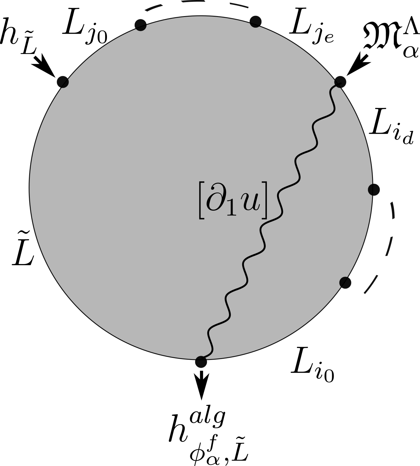
Figure 4.2. The counts defining (4.8)

Proof.

By Lemma 4.3, it suffices to prove the corresponding statement for $h^{alg}_{\phi_{\alpha}^{f},\tilde{L}}$. We define a map

(4.8) $$h_{\tilde{L}}\otimes_{{\mathcal{F}}(M,\Lambda)}\mathfrak{M}_{f\alpha}^{\Lambda}\to h^{alg}_{\phi^{f}_{\alpha},\tilde{L}}$$

in a way very similar to (3.26). Namely, send

(4.9) $$(x\otimes x_{1}\otimes\dots\otimes x_{k}\otimes x^{\prime};x_{1}^{\prime},\dots x_{l}^{\prime})$$

to the sum

(4.10) $$\sum\pm T^{E(u)}T^{f\alpha([\partial_{1}u])}.y$$

where $[\partial_{1}u]$ denote the $u$-image of the part of boundary of the disc from $\mathfrak{M}^{\Lambda}_{f\alpha}$-input $x$ to output $y$ concatenated with paths from base point of $M$. See Figure 4.2 (the wavy line is homotopic to mentioned part of the boundary). One can check that (4.8) is an $A_{\infty}$-module homomorphism in a way similar to (3.25) by considering the degenerations of discs in Figure 4.2 analogous to Figure 3.5. When $f=0$, (4.8) is a quasi-isomorphism as its cone is the standard bar resolution of $h_{\tilde{L}}$. Also, (4.8) can be thought as the specialization of a map of families

(4.11) $$h_{\tilde{L}}\otimes_{{\mathcal{F}}(M,\Lambda)}\mathfrak{M}_{\alpha}^{\Lambda}\to h^{alg}_{\phi_{\alpha},\tilde{L}}$$

at $z=T^{f}$, which can be defined by replacing (4.10) by $\sum\pm T^{E(u)}z^{\alpha([\partial_{1}u])}.y$.

We want to apply a similar semi-continuity argument as in the proof that (3.25) is a quasi-isomorphism to show (4.8) is a quasi-isomorphism for small $|f|$. For this, we want to apply Lemma A.5. Note the quasi-isomorphism of families

(4.12) $$h_{\tilde{L}}\otimes_{{\mathcal{F}}(M,\Lambda)}\mathfrak{M}_{\alpha}^{\Lambda}\simeq h_{\tilde{L}}\otimes_{{\mathcal{F}}(M,\Lambda)}\mathfrak{M}_{\alpha}^{\Lambda}\otimes_{{\mathcal{F}}(M,\Lambda)}{\mathcal{F}}(M,\Lambda)$$

where the last ${\mathcal{F}}(M,\Lambda)$ denotes the diagonal bimodule of the category denoted in the same way. Since the category ${\mathcal{F}}(M,\Lambda)$ is smooth, its diagonal bimodule is quasi-isomorphic to a direct summand of an iterated cone of Yoneda bimodules; hence, (4.12) is quasi-isomorphic to a direct summand of an iterated cone of right modules of the form

(4.13) $$h_{\tilde{L}}\otimes_{{\mathcal{F}}(M,\Lambda)}\mathfrak{M}_{\alpha}^{\Lambda}\otimes_{{\mathcal{F}}(M,\Lambda)}(h^{L_{i}}\otimes h_{L_{j}})\simeq\mathfrak{M}^{\Lambda}_{\alpha}(L_{i},\tilde{L})\otimes h_{L_{j}}$$

where $h^{L_{i}}\otimes h_{L_{j}}$ is a Yoneda bimodule, and $\mathfrak{M}^{\Lambda}_{\alpha}(L_{i},\tilde{L})$ is a free finite complex over $\Lambda\{z^{\mathbb{R}}\}$ (we can extend the category ${\mathcal{F}}(M,\Lambda)$ by $\tilde{L}$ after making it transverse to all $L_{i}$ and $\mathfrak{M}^{\Lambda}_{\alpha}$ also naturally extends in the same concrete way). Therefore, one can represent the cone of (4.11) evaluated at any object $L_{k}$ of ${\mathcal{F}}(M,\Lambda)$ as a complex satisfying the assumptions of Lemma A.5. Since we know this cone vanishes at $z=1$, we conclude the proof that (4.11) is a quasi-isomorphism when evaluated at $z=T^{f}$ for small $|f|$, i.e. (4.8) is a quasi-isomorphism by Lemma A.5.

Now, define

(4.14) $$h_{\phi^{f}_{\alpha},\tilde{L}}^{alg}\otimes_{{\mathcal{F}}(M,\Lambda)}\mathfrak{M}_{-f\alpha}^{\Lambda}\to h_{\tilde{L}}$$

similarly by replacing (4.10) by $\sum\pm T^{E(u)}T^{f\alpha([\partial_{l,m}u])}.y$, where we define $[\partial_{l,m}u]\in H_{1}(M;{\mathbb{Z}})$ to be the class obtained by concatenating the path from $h_{\phi^{f}_{\alpha},\tilde{L}}^{alg}$ input ($h_{\tilde{L}}$ input in Figure 4.2) to $\mathfrak{M}_{-f\alpha}^{\Lambda}$ input ($\mathfrak{M}_{\alpha}^{\Lambda}$ input in Figure 4.2) with the fixed paths to the base point. It is not hard to check that (4.14) is also an $A_{\infty}$-module homomorphism, and it is a quasi-isomorphisms when $f=0$. Similarly, (4.14) extends to a map of families

(4.15) $$h_{\phi_{\alpha},\tilde{L}}^{alg}\otimes_{{\mathcal{F}}(M,\Lambda)}\mathfrak{M}_{-\alpha}^{\Lambda}\to h_{\tilde{L}}$$

where $\mathfrak{M}_{-\alpha}^{\Lambda}$ is defined by the obvious modification of $\mathfrak{M}_{\alpha}^{\Lambda}$. The same proof applies to show (4.14) is a quasi-isomorphism for small $|f|$. The only difference is that one has to use the resolution of the diagonal bimodule ${\mathcal{F}}(M,\Lambda)$ on both appearances in the following

(4.16) $$h_{\phi_{\alpha},\tilde{L}}^{alg}\otimes_{{\mathcal{F}}(M,\Lambda)}{\mathcal{F}}(M,\Lambda)\otimes_{{\mathcal{F}}(M,\Lambda)}\mathfrak{M}_{-\alpha}^{\Lambda}\otimes_{{\mathcal{F}}(M,\Lambda)}{\mathcal{F}}(M,\Lambda)$$

∎

An immediate corollary of Lemma 4.6 is the following:

Corollary 4.7.

The Yoneda module $h_{\phi^{f}_{\alpha}(L^{\prime})}$ is definable over ${\mathcal{F}}(M,K)$ for $f\in{\mathbb{Z}}_{(p)}$ such that $|f|$ is sufficiently small. In other words, there exists a perfect module over ${\mathcal{F}}(M,K)$ such that one obtains a module quasi-isomorphic to $h_{\phi^{f}_{\alpha}(L^{\prime})}$ after base change to $\Lambda$ (we do not make any uniqueness statement though).

Proof.

Consider the perfect module $h_{L^{\prime}}\otimes_{{\mathcal{F}}(M,K)}\mathfrak{M}^{K}_{\alpha}|_{z=T^{f}}$ over ${\mathcal{F}}(M,K)$, which is well-defined as $f\in{\mathbb{Z}}_{(p)}$ and $T^{f\alpha(C)}\in K$. Once one extends the coefficients to $\Lambda$, one obtains $h_{L^{\prime}}\otimes_{{\mathcal{F}}(M,\Lambda)}\mathfrak{M}^{\Lambda}_{f\alpha}$, which is quasi-isomorphic to $h_{\phi^{f}_{\alpha}(L^{\prime})}$ by Lemma 4.6. ∎

Remark 4.8.

One could use Lemma 4.3 directly to prove the corollary. Since the sum defining $h_{L^{\prime}}$ is assumed to be finite, (4.4) also remains finite. Therefore, if $f\in{\mathbb{Z}}_{(p)}$, $h^{alg}_{\phi^{f}_{\alpha},L^{\prime}}$ is definable over ${\mathcal{F}}(M,K)$ in the sense above, and by Lemma 4.3, it becomes quasi-isomorphic to $h_{\phi^{f}_{\alpha}(L^{\prime})}$ after extending the coefficients $K\subset\Lambda$.

We can drop the assumption that $|f|$ is small from Lemma 4.6 after modifying it as follows:

Lemma 4.9.

For any $f>0$ and $\tilde{L}$, one can find a sequence of numbers $0=s_{0}<s_{1}<\dots<s_{r}=f$ such that

(4.17) $$h_{\phi^{f}_{\alpha}(\tilde{L})}\simeq h_{\tilde{L}}\otimes_{{\mathcal{F}}(M,\Lambda)}\mathfrak{M}_{(s_{1}-s_{0})\alpha}^{\Lambda}\otimes_{{\mathcal{F}}(M,\Lambda)}\mathfrak{M}_{(s_{2}-s_{1})\alpha}^{\Lambda}\dots\otimes_{{\mathcal{F}}(M,\Lambda)}\mathfrak{M}_{(s_{r}-s_{r-1})\alpha}^{\Lambda}$$

Similarly, when $f<0$, there is a sequence $0=s_{0}>s_{1}>\dots>s_{r}=f$ such that (4.17) is satisfied. Moreover, if $f\in{\mathbb{Z}}_{(p)}$, resp. $f\in p^{n}{\mathbb{Z}}_{(p)}$ then one can assume all $s_{i}\in{\mathbb{Z}}_{(p)}$, resp. $s_{i}\in p^{n}{\mathbb{Z}}_{(p)}$.

Proof.

Without loss of generality, assume $f>0$ and consider the isotopy $\phi_{\alpha}^{s}(\tilde{L}),s\in[0,f]$. By Lemma 4.6, any $s\in[0,f]$ has an open neighborhood $(s-\epsilon,s+\epsilon)$ such that

(4.18) $$h_{\phi_{\alpha}^{s}(\tilde{L})}\simeq h_{\phi_{\alpha}^{s^{\prime}}(\tilde{L})}\otimes_{{\mathcal{F}}(M,\Lambda)}\mathfrak{M}_{(s-s^{\prime})\alpha}^{\Lambda}\atop h_{\phi_{\alpha}^{s^{\prime\prime}}(\tilde{L})}\simeq h_{\phi_{\alpha}^{s}(\tilde{L})}\otimes_{{\mathcal{F}}(M,\Lambda)}\mathfrak{M}_{(s^{\prime\prime}-s)\alpha}^{\Lambda}$$

for $s^{\prime},s^{\prime\prime}\in(s-\epsilon,s+\epsilon)$.

Assume $\epsilon$ is small enough so that Lemma 3.5 is also satisfied for $|f|,|f^{\prime}|<\epsilon$, i.e. $\mathfrak{M}_{f\alpha}^{\Lambda}\otimes_{{\mathcal{F}}(M,\Lambda)}\mathfrak{M}_{f^{\prime}\alpha}^{\Lambda}\simeq\mathfrak{M}_{(f+f^{\prime})\alpha}^{\Lambda}$ for $|f|,|f^{\prime}|<\epsilon$. Then

(4.19) $$h_{\phi_{\alpha}^{s^{\prime\prime}}(\tilde{L})}\simeq h_{\phi_{\alpha}^{s}(\tilde{L})}\otimes_{{\mathcal{F}}(M,\Lambda)}\mathfrak{M}_{(s^{\prime\prime}-s)\alpha}^{\Lambda}\simeq$$

(4.20) $$h_{\phi_{\alpha}^{s^{\prime}}(\tilde{L})}\otimes_{{\mathcal{F}}(M,\Lambda)}\mathfrak{M}_{(s-s^{\prime})\alpha}^{\Lambda}\otimes_{{\mathcal{F}}(M,\Lambda)}\mathfrak{M}_{(s^{\prime\prime}-s)\alpha}^{\Lambda}\simeq$$

(4.21) $$h_{\phi_{\alpha}^{s^{\prime}}(\tilde{L})}\otimes_{{\mathcal{F}}(M,\Lambda)}\mathfrak{M}_{(s^{\prime\prime}-s^{\prime})\alpha}^{\Lambda}$$

for any $s^{\prime},s^{\prime\prime}\in(s-\epsilon,s+\epsilon)$. The last equivalence comes from Lemma 3.5.

Call such $s^{\prime},s^{\prime\prime}$ algebraically related. One can cover $[0,f]$ by finitely many such small intervals, and this gives a sequence $0=s_{0}<s_{1}<\dots<s_{r}=f$ such that $s_{i}$ and $s_{i+1}$ are algebraically related, concluding the proof. We could choose any $(r+1)$-tuple $0=s_{0}^{\prime}<\dots<s_{r}^{\prime}=f$ sufficiently close to $0=s_{0}<s_{1}<\dots<s_{r}=f$, in particular we can assume they are in ${\mathbb{Z}}_{(p)}$, resp. $p^{n}{\mathbb{Z}}_{(p)}$. ∎

Corollary 4.10.

If $f\in p^{n}{\mathbb{Z}}_{(p)}$, then

(4.22) $$h_{\phi_{\alpha}^{f}(L^{\prime})}\simeq h_{L^{\prime}}\otimes_{{\mathcal{F}}(M,\Lambda)}\mathfrak{M}^{\Lambda}_{f\alpha}$$

Proof.

Assume $f>0$ without loss of generality. If $f\in p^{n}{\mathbb{Z}}_{(p)}$, we can choose $0=s_{0}<\dots<s_{r}=f$ in Lemma 4.9 from $p^{n}{\mathbb{Z}}_{(p)}$. Therefore, $s_{i+1}-s_{i}\in p^{n}{\mathbb{Z}}_{(p)}$ and $\mathfrak{M}_{f\alpha}^{\Lambda}\otimes_{{\mathcal{F}}(M,\Lambda)}\mathfrak{M}_{f^{\prime}\alpha}^{\Lambda}\simeq\mathfrak{M}_{(f+f^{\prime})\alpha}^{\Lambda}$ holds when $f,f^{\prime}\in p^{n}{\mathbb{Z}}_{(p)}$ by Corollary 3.24. This fact, together with (4.17) implies the corollary. ∎

Observe that if one confines themselves to the case $f\in p^{n}{\mathbb{Z}}_{(p)}$, one can prove Lemma 4.9 and Corollary 4.10 by using Corollary 3.24, rather than Lemma 3.5.

Proof of Proposition 4.1.

Let $f\in p^{n}{\mathbb{Z}}_{(p)}$. Then by Corollary 4.10

(4.23) $$h_{\phi_{\alpha}^{-f}(L^{\prime})}\simeq h_{L^{\prime}}\otimes_{{\mathcal{F}}(M,\Lambda)}\mathfrak{M}^{\Lambda}_{-f\alpha}$$

Applying $(\cdot)\otimes_{{\mathcal{F}}(M,\Lambda)}h^{L}$ to both sides of (4.23), we obtain

(4.24) $$h_{\phi_{\alpha}^{-f}(L^{\prime})}\otimes_{{\mathcal{F}}(M,\Lambda)}h^{L}\simeq h_{L^{\prime}}\otimes_{{\mathcal{F}}(M,\Lambda)}\mathfrak{M}^{\Lambda}_{-f\alpha}\otimes_{{\mathcal{F}}(M,\Lambda)}h^{L}$$

Moreover,

(4.25) $$CF(L,\phi_{\alpha}^{-f}(L^{\prime}))\simeq h_{\phi_{\alpha}^{-f}(L^{\prime})}\otimes_{{\mathcal{F}}(M,\Lambda)}h^{L}$$

by Lemma 2.12. Combining these, we get

(4.26) $$CF(\phi_{\alpha}^{f}(L),L^{\prime})\simeq CF(L,\phi_{\alpha}^{-f}(L^{\prime}))\simeq h_{L^{\prime}}\otimes_{{\mathcal{F}}(M,\Lambda)}\mathfrak{M}^{\Lambda}_{-f\alpha}\otimes_{{\mathcal{F}}(M,\Lambda)}h^{L}$$

which proves (4.1) as

(4.27) $$h_{L^{\prime}}\otimes_{{\mathcal{F}}(M,\Lambda)}\mathfrak{M}^{\Lambda}_{-f\alpha}\otimes_{{\mathcal{F}}(M,\Lambda)}h^{L}\simeq\mathfrak{M}^{\Lambda}_{-f\alpha}(L,L^{\prime})$$

The statement about the dimension is straightforward, namely the proper module

(4.28) $$h_{L^{\prime}}\otimes_{{\mathcal{F}}(M,K)}\mathfrak{M}^{K}_{\alpha}|_{z=T^{-f}}\otimes_{{\mathcal{F}}(M,K)}h^{L}$$

is well defined. By extending coefficients under $K\hookrightarrow\Lambda$ one obtains

(4.29) $$h_{L^{\prime}}\otimes_{{\mathcal{F}}(M,\Lambda)}\mathfrak{M}^{\Lambda}_{\alpha}|_{z=T^{-f}}\otimes_{{\mathcal{F}}(M,\Lambda)}h^{L}$$

on the one hand, and by extending coefficients under $K\hookrightarrow{\mathbb{Q}}_{p}$, one obtains

(4.30) $$h_{L^{\prime}}\otimes_{{\mathcal{F}}(M,{\mathbb{Q}}_{p})}\mathfrak{M}^{{\mathbb{Q}}_{p}}_{\alpha}|_{t=-f}\otimes_{{\mathcal{F}}(M,{\mathbb{Q}}_{p})}h^{L}$$

Base change under field extensions do not change the dimensions of cohomology groups, and this finishes the proof. ∎

Remark 4.11.

One can generalize Proposition 4.1 to all $f\in{\mathbb{Z}}_{(p)}$ by using an argument that will also be used in the proof of Theorem 1.1.

We can now prove the main theorem:

Theorem 1.1.

Under given assumptions, the rank of $HF(\phi^{k}(L),L^{\prime}),k\in{\mathbb{N}}$ is constant except for finitely many $k$.

Proof.

Recall that we assume $\phi=\phi_{\alpha}^{1}$ without loss of generality. By Proposition 4.1, the rank of $HF(\phi^{k}(L),L^{\prime})$ is equal to the rank of

(4.31) $$H^{*}\big{(}h_{L^{\prime}}\otimes_{{\mathcal{F}}(M,{\mathbb{Q}}_{p})}\mathfrak{M}^{{\mathbb{Q}}_{p}}_{\alpha}|_{t=-k}\otimes_{{\mathcal{F}}(M,{\mathbb{Q}}_{p})}h^{L}\big{)}$$

as long as $k\equiv 0\,(mod\,p^{n})$. On the other hand, the following is a finitely generated graded module over ${\mathbb{Q}}_{p}\langle t\rangle$:

(4.32) $$H^{*}\big{(}h_{L^{\prime}}\otimes_{{\mathcal{F}}(M,{\mathbb{Q}}_{p})}\mathfrak{M}^{{\mathbb{Q}}_{p}}_{\alpha}\otimes_{{\mathcal{F}}(M,{\mathbb{Q}}_{p})}h^{L}\big{)}$$

whose restriction to $t=-k$ gives (4.31). More precisely, let $C$ be a free, finite complex over ${\mathbb{Q}}_{p}\langle t\rangle$ that is quasi-isomorphic to $h_{L^{\prime}}\otimes_{{\mathcal{F}}(M,{\mathbb{Q}}_{p})}\mathfrak{M}^{{\mathbb{Q}}_{p}}_{\alpha}\otimes_{{\mathcal{F}}(M,{\mathbb{Q}}_{p})}h^{L}$ (which exists by [Ked04, Proposition 6.5] as before). Then, (4.31) is isomorphic to $H^{*}(C\xrightarrow{-k}C)$, i.e. the cohomology of the cone of multiplication by $-k$, and it is an extension of $H^{*}(C)/(-k)H^{*}(C)$ and $ker(-k)\subset H^{*}(C)[1]$ (one can use resolution ${\mathbb{Q}}_{p}\langle t\rangle\xrightarrow{-k}{\mathbb{Q}}_{p}\langle t\rangle$ of the structure sheaf of $-k$, or Tor spectral sequence, or equivalently the universal coefficient theorem). Since the Tate algebra ${\mathbb{Q}}_{p}\langle t\rangle$ is a PID (see for instance [Bos14, Section 2, Cor 10]), $H^{*}(C)$ admits a description as the sum of a free module and a torsion module supported at finitely many points. Hence, the rank of both $H^{*}(C)/(-k)H^{*}(C)$ and $ker(-k)$ are constant except for finitely many $k\in{\mathbb{Z}}_{p}$ (thus, the rank of (4.31) also satisfies this). Combining this with the previous statement, we conclude that the rank of $HF(\phi^{k}(L),L^{\prime})$ is constant among $k\in p^{n}{\mathbb{Z}}_{(p)}$ with finitely many exceptions.

Now choose $f_{1},f_{2},\dots,f_{p^{n}-1}\in{\mathbb{Z}}_{(p)}$ such that $f_{i}\equiv i\,(mod\,p^{n})$ and $|f_{i}|$ is small so that Lemma 4.3 and Lemma 4.6 hold for $\tilde{L}=L^{\prime}$ and $f=-f_{i}$. In other words, $h^{alg}_{\phi^{-f_{i}}_{\alpha},L^{\prime}}\simeq h_{\phi^{-f_{i}}_{\alpha}(L^{\prime})}\simeq h_{L^{\prime}}\otimes_{{\mathcal{F}}(M,\Lambda)}\mathfrak{M}^{\Lambda}_{-f_{i}\alpha}$. In particular, $h_{\phi^{-f_{i}}_{\alpha}(L^{\prime})}$ is definable over ${\mathcal{F}}(M,K)$, and therefore over ${\mathcal{F}}(M,{\mathbb{Q}}_{p})$ (see Corollary 4.7). Given $f\equiv f_{i}\,(mod\,p^{n})$, one can prove

(4.33) $$h_{\phi^{-f}_{\alpha}(L^{\prime})}\simeq h_{L^{\prime}}\otimes_{{\mathcal{F}}(M,\Lambda)}\mathfrak{M}^{\Lambda}_{-f_{i}\alpha}\otimes_{{\mathcal{F}}(M,\Lambda)}\mathfrak{M}^{\Lambda}_{(-f+f_{i})\alpha}$$

as a corollary of Lemma 4.9, similar to Corollary 4.10. Then one can simply follow the proof of Proposition 4.1 to prove that the rank of $HF(\phi_{\alpha}^{f}(L),L^{\prime})$ is the same as the rank of

(4.34) $$H^{*}\big{(}h_{L^{\prime}}\otimes_{{\mathcal{F}}(M,{\mathbb{Q}}_{p})}\mathfrak{M}^{{\mathbb{Q}}_{p}}_{-f_{i}\alpha}\otimes_{{\mathcal{F}}(M,{\mathbb{Q}}_{p})}\mathfrak{M}^{{\mathbb{Q}}_{p}}_{(-f+f_{i})\alpha}\otimes_{{\mathcal{F}}(M,{\mathbb{Q}}_{p})}h^{L}\big{)}$$

i.e. the rank of of ${\mathbb{Q}}_{p}\langle t\rangle$-module (or ${\mathbb{Q}}_{p}\langle t/p^{n}\rangle$-module, after restriction)

(4.35) $$H^{*}\big{(}h_{L^{\prime}}\otimes_{{\mathcal{F}}(M,{\mathbb{Q}}_{p})}\mathfrak{M}^{{\mathbb{Q}}_{p}}_{-f_{i}\alpha}\otimes_{{\mathcal{F}}(M,{\mathbb{Q}}_{p})}\mathfrak{M}^{{\mathbb{Q}}_{p}}_{\alpha}\otimes_{{\mathcal{F}}(M,{\mathbb{Q}}_{p})}h^{L}\big{)}$$

at point $t=-f+f_{i}$. This allows one to conclude the rank of $HF(\phi_{\alpha}^{f}(L),L^{\prime})$ is constant among all but finitely many $f$ satisfying $f\equiv f_{i}\,(mod\,p^{n})$. Therefore, the rank of $HF(\phi_{\alpha}^{f}(L),L^{\prime}),f\in{\mathbb{Z}}$ is periodic of period (dividing) $p^{n}$, except for finitely many $f\in{\mathbb{Z}}$.

Notice, we can replace $p$ by another prime $p^{\prime}>2$, to conclude this sequence is periodic of period $(p^{\prime})^{n^{\prime}}$ for some $n^{\prime}$, except finitely many terms. Since, $p$ and $p^{\prime}$ are coprime, this implies that rank of $HF(\phi_{\alpha}^{f}(L),L^{\prime}),f\in{\mathbb{Z}}$ is constant outside finitely many $f$. ∎

Remark 4.12.

The proof actually implies that the rank of $HF(\phi_{\alpha}^{f}(L),L^{\prime})$ is constant except for finitely many $f\in{\mathbb{Z}}_{(pp^{\prime})}=\{\frac{a}{b}:a,b\in{\mathbb{Z}},p\nmid b,p^{\prime}\nmid b\}$. Applying this version to $r\alpha,r\in{\mathbb{R}}$ in place of $\alpha$ implies that rank of $HF(\phi_{\alpha}^{rf}(L),L^{\prime})$ is constant except for finitely many $f\in{\mathbb{Z}}_{(pp^{\prime})}$. However, from this, we cannot immediately conclude that the rank of $HF(\phi_{\alpha}^{f}(L),L^{\prime}),f\in{\mathbb{R}}$ is constant except for finitely many $f\in{\mathbb{R}}$, as the union of all these finite sets corresponding to classes in ${\mathbb{R}}/{\mathbb{Z}}_{(pp^{\prime})}$ may still be infinite.

Remark 4.13.

Under the assumption that $L$ and $L^{\prime}$ are Bohr-Sommerfeld monotone, one can assume they are two of the fixed generators $\{L_{i}\}$ without loss of generality. Therefore, it is possible to calculate the rank of $h_{L^{\prime}}\otimes_{{\mathcal{F}}(M,{\mathbb{Q}}_{p})}\mathfrak{M}^{{\mathbb{Q}}_{p}}_{\alpha}\otimes_{{\mathcal{F}}(M,{\mathbb{Q}}_{p})}h^{L}$ as the dimension of the cohomology of $\mathfrak{M}^{{\mathbb{Q}}_{p}}_{\alpha}(L,L^{\prime})$ or $\mathfrak{M}^{K}_{\alpha}(L,L^{\prime})$. In particular, if $L\cap L^{\prime}=\emptyset$, then this complex is $0$, and Proposition 4.1 implies $HF(\phi^{k}(L),L^{\prime};\Lambda)=0$ for all $k\in p^{n}{\mathbb{Z}}_{(p)}$. As mentioned in Remark 3.23, it is likely that the group-like property holds over the larger base $Sp({\mathbb{Q}}_{p}\langle t\rangle)$, that would let one to conclude the same for all $k\in{\mathbb{Z}}_{(p)}$. Therefore, one would have $HF(\phi^{1}_{\alpha}(L),L^{\prime};\Lambda)=0$ for all $\alpha$. This may sound to contradict the theorem; for instance, by letting $L^{\prime}=\phi^{1}_{\alpha}(L)$. However, $L$ and $\phi^{1}_{\alpha}(L)$ cannot be Bohr-Sommerfeld at the same time, i.e. this remark does not apply in this case. As we will explain, one can get rid of Bohr-Sommerfeld assumption on $L$ and $L^{\prime}$ by passing to a finitely generated extension $K\subset\tilde{K}$ over which $h_{L^{\prime}}$ and $h^{L}$ are definable. However, this does not mean that the modules $h_{L^{\prime}}$ and $h^{L}$ (defined in the usual way as in Section 2, not as Yoneda modules of twisted complexes over ${\mathcal{F}}(M,\Lambda)$) have coefficients in $K$ or $\tilde{K}$.

Dropping the assumption that $L$ and $L^{\prime}$ are Bohr-Sommerfeld monotone

We briefly explain how to drop the assumption that $L$ and $L^{\prime}$ are Bohr-Sommerfeld, while holding the assumption that they are monotone and have minimal Maslov number $3$. The idea is simple: one can represent the modules $h_{L^{\prime}}$ and $h^{L}$ as iterated cones/twisted complexes of Yoneda modules of $\{L_{i}\}$. Since the data to define a twisted complex is finite, these modules are definable over a finitely generated extension of $K$, if not $K$ itself.

More precisely, represent $L^{\prime}$ as an element of $tw^{\pi}({\mathcal{F}}(M,\Lambda))$, i.e. $L^{\prime}\simeq(\bigoplus_{k}L_{i_{k}},\sigma,\pi)$, where $\sigma$ is the differential of the twisted complex and $\pi$ is the idempotent. Write components of $\sigma$ and $\pi$ as linear combinations of the generators of $CF(L_{i},L_{j})$. It is easy to see that one must add only finitely many elements from $\Lambda$ to the subfield $K$ to include the coefficients of these linear expressions. In other words, there exists a finitely generated extension $K\subset\tilde{K}$ such that $\sigma$ and $\pi$, and hence this twisted complex is defined over ${\mathcal{F}}(M,\tilde{K})$— the category obtained from ${\mathcal{F}}(M,K)$ via base change along $K\to\tilde{K}$. Let $h^{\prime}_{L^{\prime}}$ denote the image of this twisted complex under Yoneda embedding. By construction, $h^{\prime}_{L^{\prime}}$ turns into a module quasi-isomorphic to $h_{L^{\prime}}$, when we base change under $\tilde{K}\subset\Lambda$. Denote this module by $h^{\prime}_{L^{\prime}}$ as well. Similarly, $h^{L}$ is also definable over a finitely generated extension of $K$, i.e. by further extending $\tilde{K}$ by finitely many elements, one can ensure that there exists a left ${\mathcal{F}}(M,\tilde{K})$-module $h^{\prime L}$ that becomes quasi-isomorphic to $h^{L}$ after base change along $\tilde{K}\subset\Lambda$.

Since $\tilde{K}$ is finitely generated and countable, one can find a finite (not only finitely generated) extension ${\mathbb{Q}}_{p}^{\prime}$ of ${\mathbb{Q}}_{p}$ and a map $\tilde{\mu}:\tilde{K}\to{\mathbb{Q}}_{p}^{\prime}$ extending $\mu:K\to{\mathbb{Q}}_{p}$. For this one can first extend $\mu$ to a map to ${\mathbb{Q}}_{p}$ from a maximal purely transcendental extension of $K$ inside $\tilde{K}$ (by choosing a set of elements of ${\mathbb{Q}}_{p}$ that are algebraically independent over $\mu(K)$). Then, $\tilde{K}$ is finite over this extension of $K$, and there exists a finite extension ${\mathbb{Q}}_{p}^{\prime}$ of ${\mathbb{Q}}_{p}$ and a map $\tilde{\mu}:\tilde{K}\to{\mathbb{Q}}_{p}^{\prime}$, whose restriction to $K$ is equal to $\mu$.

${\mathbb{Q}}_{p}^{\prime}$ carries a unique discrete valuation extending that on ${\mathbb{Q}}_{p}$ (see [Shi10, Theorem 9.5]), and one can use the base change under ${\mathbb{Q}}_{p}\langle t\rangle\to{\mathbb{Q}}_{p}^{\prime}\langle t\rangle$ to obtain a family $\mathfrak{M}^{{\mathbb{Q}}_{p}^{\prime}}_{\alpha}$ over the latter that is group-like over ${\mathbb{Q}}_{p}^{\prime}\langle t/p^{n}\rangle$. The proof of Proposition 4.1 still applies and we have

(4.36) $$dim_{\Lambda}\big{(}HF(\phi^{k}(L),L^{\prime})\big{)}=dim_{{\mathbb{Q}}_{p}^{\prime}}\big{(}H^{*}\big{(}h^{\prime}_{L^{\prime}}\otimes_{{\mathcal{F}}(M,{\mathbb{Q}}_{p}^{\prime})}\mathfrak{M}^{{\mathbb{Q}}_{p}^{\prime}}_{\alpha}|_{t=-f}\otimes_{{\mathcal{F}}(M,{\mathbb{Q}}_{p}^{\prime})}h^{\prime L}\big{)}\big{)}$$

for all $k\in p^{n}{\mathbb{Z}}_{(p)}$. This dimension is constant for all but finitely many $k$ as before.

Replacing $L^{\prime}$ by $\phi^{-i}(L^{\prime})$, where $i=0,1,\dots p^{n}-1$, we see that $dim_{\Lambda}\big{(}HF(\phi^{k}(L),L^{\prime})\big{)}$ is constant for all but finitely many $k\in i+p^{n}{\mathbb{Z}}_{(p)}$. Therefore, $dim_{\Lambda}\big{(}HF(\phi^{k}(L),L^{\prime})\big{)}$ is $p^{n}$ periodic for all but finitely many $k\in{\mathbb{Z}}$, and by replacing $p$ by another prime, we see that this dimension is actually constant among $k\in{\mathbb{Z}}$ except finitely many. This concludes the proof of Theorem 1.1 without the Bohr-Sommerfeld assumption on $L$ and $L^{\prime}$.

Remark 4.14.

Observe that we did not need to use $f_{i}\in i+p^{n}{\mathbb{Z}}_{(p)}$ such that $|f_{i}|$ is small as we did not need an algebraic replacement for $h_{\phi^{-i}(L^{\prime})}$.

5. Generic $\alpha$ and the proof of Theorem 1.5

In this section, we will explain a way to construct group-like $p$-adic families of bimodules (i.e. “analytic ${\mathbb{Z}}_{p}$-actions”) without the assumption of monotonicity of $M$ at the cost of assuming $\alpha$ is generic. Using this, we will deduce Theorem 1.5.

The main reason we had to assume monotonicity was that, we had no way of ensuring convergence for an infinite series of the form (3.24) as well as (3.27) in ${\mathbb{Q}}_{p}$. One could try to choose the map $\mu:K\to{\mathbb{Q}}_{p}$ so that $\mu(T^{E(u)})\in p{\mathbb{Z}}_{p}$ and $\mu(T^{\alpha([\partial_{h}u])})\in 1+p{\mathbb{Z}}_{p}$, but such a map may not exist if there are algebraic relations between the elements of the form $T^{E(u)}$ and $T^{\alpha([\partial_{h}u])}$. On the other hand, for generic $[\alpha]\in H^{1}(M,{\mathbb{R}})$, there are no such algebraic relations. Therefore, one can define the embedding of the field of definition into ${\mathbb{Q}}_{p}$ such that the images of $T^{E(u)}$ converge in $p$-adic topology, just like $T^{E(u)}$ converging in $T$-adic topology by Gromov compactness.

Our construction works in the general setting as long as one assumes the Fukaya category is well defined with coefficients in $\Lambda$, and it is smooth and proper. We assume there exists a finite set of Lagrangians $L_{1},\dots,L_{m}$ that are all tautologically unobstructed and that generate the Fukaya category (we actually make the stronger assumption that $L_{i}$ bound no disc with Maslov index $2$). We denote the span of $L_{1},\dots,L_{m}$ by ${\mathcal{F}}(M,\Lambda)$. Two natural examples of such $M$ are an elliptic curve and product of two elliptic curves. Let $L,L^{\prime}$ be two branes satisfying Assumption 1.6, which are represented by elements of $tw^{\pi}({\mathcal{F}}(M,\Lambda))$ by generation assumption. Assume $L_{i},L,L^{\prime}$ are pairwise transverse.

Fix an almost complex structure on $M$. Our first goal is to embed the additive semi-group spanned by $E(u)>0$ into the multiplicative semi-group $p{\mathbb{Z}}_{p}$. For this, we prove that there exists a discrete free submonoid of ${\mathbb{R}}_{\geq 0}$ that contains energies of all pseudo-holomorphic curves in $M$ with boundary on $L_{i},L,L^{\prime}$:

Lemma 5.1.

There exists rationally independent elements

(5.1) $$E_{1},\dots,E_{n}\in{\mathbb{R}}_{>0}\cap\omega_{M}(H_{2}(M,L\cup L^{\prime}\cup\bigcup_{i}L_{i};{\mathbb{Q}}))$$

such that the monoid spanned by them contain the energy of every non-constant pseudo-holomorphic curve.

Proof.

For simplicity, we work with curves with boundary on a single Lagrangian $L$. Let $J$ denote the compatible almost complex structure. Let $\omega_{1},\dots,\omega_{n^{\prime}}$ denote closed $2$-forms that are obtained by small perturbations of $\omega_{M}$ and that satisfy:

1. $\omega_{i}$ are still symplectic and tamed by $J$

2. $\omega_{i}|_{L}=0$ for all $i$ and $\{[\omega_{i}]\}$ form a basis of $H^{2}(M,L;{\mathbb{Q}})$ (in particular they are rational)

3. $[\omega_{M}]\in H^{2}(M,L;{\mathbb{R}})$ is in the convex hull of the rays generated by $[\omega_{i}]$

(1) can be ensured since $M$ is compact; therefore, small perturbations of $\omega_{M}$ remain symplectic and are still tamed by $J$. For other conditions, first choose closed $2$-forms $\theta_{1}=\omega_{M},\theta_{2},\dots,\theta_{n^{\prime}}$ representing a basis of $H^{2}(M,L;{\mathbb{R}})$ and identify the space $\bigoplus_{i}{\mathbb{R}}.\theta_{i}$ with $H^{2}(M,L;{\mathbb{R}})$. Consider a small open cone around $\omega_{M}$ inside this finite dimensional space, and choose $\omega_{i}$ among $1$-forms sufficiently close to $\omega_{M}$ and representing rational classes (rational classes of $1$-forms are dense). Then, it is easy to make this choice so that (2) and (3) are satisfied.

Since each $\omega_{i}$ is symplectic and tamed by $J$, the energy of a non-constant pseudo-holomorphic curve representing class $\beta\in H_{2}(M,L;{\mathbb{Z}})$ with respect to the metric $g_{i}(v,w)=\frac{1}{2}(\omega_{i}(v,Jw)+\omega_{i}(w,Jv))$ is still strictly positive and can be calculated as $\omega_{i}(\beta)$. Furthermore, there exists a natural number $N$ such that $\omega_{i}(H_{2}(M,L;{\mathbb{Z}}))\subset\frac{1}{N}{\mathbb{Z}}$. Choose a common $N$ for all $\omega_{i}$.

Consider the set

(5.2) $$\{\beta\in H_{2}(M,L;{\mathbb{Q}}):\omega_{i}(\beta)>0\text{ and }\omega_{i}(\beta)\in\frac{1}{N}{\mathbb{Z}}\text{ for all }i\}\cup\{0\}$$

If we use $(\omega_{i})_{i}$ to identify $H_{2}(M,L;{\mathbb{Q}})$ with ${\mathbb{Q}}^{n^{\prime}}$, then (5.2) corresponds to $(\frac{1}{N}{\mathbb{Z}}_{+})^{n^{\prime}}\cup\{0\}$. Therefore, (5.2) is a finitely generated submonoid of $H_{2}(M,L;{\mathbb{Q}})$. As remarked, it contains the classes of all $J$-holomorphic curves. Also, as $\omega_{M}$ can be represented as a positive linear combination of $\omega_{i}$, the image of (5.2) under $\omega_{M}$ is a submonoid of ${\mathbb{R}}_{\geq 0}$, and it is finitely generated as (5.2) is. We conclude the proof by applying Lemma 5.2 below to the image of (5.2) under $\omega_{M}$. ∎

Lemma 5.2.

Every finitely generated additive submonoid of ${\mathbb{R}}_{\geq 0}$ can be extended in its rational span to a submonoid generated by positive, rationally independent elements.

Proof.

We proceed by induction on the number of generators. Assume the statement holds when there are less than $n$ generators. Consider an additive submonoid of ${\mathbb{R}}_{\geq 0}$ generated by $x_{1},\dots,x_{n}>0$. By induction hypothesis for $x_{1},\dots,x_{n-1}$, we can find a monoid in their rational span generated by rationally independent elements $y_{1},\dots y_{k}>0$ that contains $x_{1},\dots,x_{n-1}$. If $x_{n}$ is rationally independent of $\{y_{i}\}$, then $y_{1},\dots,y_{k},x_{n}$ is a rationally independent set of generators of a monoid containing $x_{1},\dots,x_{n}$.

Otherwise, one can write $x_{n}$ as $x_{n}=a_{1}y_{i_{1}}+\dots+a_{q}y_{i_{q}}-b_{1}y_{j_{1}}-\dots-b_{r}y_{j_{r}}$, where $a_{i}\in{\mathbb{Q}}_{+},b_{j}\in{\mathbb{Q}}_{\geq 0}$, such that the sets $\{y_{i_{1}}\dots,y_{i_{q}}\}$ and $\{y_{j_{1}},\dots,y_{j_{r}}\}$ form a partition of $\{y_{1},\dots,y_{k}\}$ (i.e. they are disjoint, and their union contains all $y_{i}$). Let $b_{1}y_{j_{1}}+\dots+b_{r}y_{j_{r}}$ be denoted by $\eta$. Since $x_{n}>0$, there exists $\lambda_{1},\dots,\lambda_{q}\in{\mathbb{Q}}_{\geq 0}$ such that $\lambda_{1}+\dots+\lambda_{q}=1$, and $a_{h}y_{i_{h}}-\lambda_{h}\eta>0$ (to see this, assume $\eta>0$ and $a_{h}y_{i_{h}}=\iota_{h}\eta$, where $\iota_{h}>0$. Thus, $\sum\iota_{h}>1$, choose $\lambda_{h}$ to be a rational partition of $1$ such that $\iota_{h}-\lambda_{h}>0$). We can find a new basis that consist of positive rational multiples of $y_{j_{g}}$ and $a_{h}y_{i_{h}}-\lambda_{h}\eta$. For instance, let $\tau_{1}\in{\mathbb{Z}}_{+}$ be the product of numerators of all $a_{h}$, and let $\tau_{2}\in{\mathbb{Z}}_{+}$ be the product of denominators of all $\lambda_{h}$ and $b_{g}$. Then, it is easy to see that the monoid spanned by positive rationally independent elements $\frac{1}{\tau_{1}}(a_{h}y_{i_{h}}-\lambda_{h}\eta),h=1,\dots,q$, $\frac{1}{\tau_{1}\tau_{2}}y_{j_{g}},g=1,\dots,r$ contain $y_{1},\dots,y_{k},x_{n}$, and thus it contains $x_{1},\dots,x_{n}$. This finishes the proof. ∎

Remark 5.3.

Lemma 5.1 is still true when we allow the almost complex structure to vary, as in [Sei08], as long as $\omega_{M}$ is rational. If we want it to hold for more general $\omega_{M}$, we have to let almost complex structures vary in a bounded way. For instance, one can choose a small neighborhood of $[\omega_{M}]$ in $H^{2}(M,{\mathbb{R}})$ whose elements are represented by symplectic forms deforming $\omega_{M}$, and consider only the almost complex structures tamed by these forms.

Remark 5.4.

Gromov compactness imply that the set of energies of non-constant pseudo-holomorphic curves is a discrete subset of ${\mathbb{R}}_{+}$; however, we are unable to use this statement to give a simpler proof of Lemma 5.1. The main difficulty is the finite generation statement, it is not true that an additive submonoid of ${\mathbb{R}}_{\geq 0}$ that lies in a finitely generated subgroup of ${\mathbb{R}}$ is always contained in a finitely generated submonoid of ${\mathbb{R}}_{\geq 0}$. For instance, consider the monoid generated by $1$ and $\sqrt{2}$. It is a discrete monoid, and we can expand it to another discrete monoid by adding an element of the set ${\mathbb{Z}}+\sqrt{2}{\mathbb{Z}}$ that is outside the original monoid (such as $3\sqrt{2}-1$). Then, we can go on by adding another element of ${\mathbb{Z}}+\sqrt{2}{\mathbb{Z}}$ from outside the monoid, to expand it further. We continue in this way, and the union of this nested sequence of monoids is a monoid that is not finitely generated. If we assume the element added at the $n^{th}$ step is larger than $n$, then this monoid is discrete.

Let ${\mathcal{E}}_{+}\subset{\mathbb{R}}_{\geq 0}$ denote the monoid spanned by $E_{1},\dots,E_{n}$. Since these generators are rationally independent, there is no algebraic relation between $T^{E_{i}}$.

Definition 5.5.

$\alpha$ is called generic if $\alpha(H_{1}(M,{\mathbb{Z}}))$ intersects the group generated by ${\mathcal{E}}_{+}$ only at $0$.

This condition is weaker than

(5.3) $$\alpha(H_{1}(M,{\mathbb{Z}}))\cap\omega_{M}(H_{2}(M,L\cup L^{\prime}\cup\bigcup_{i}L_{i};{\mathbb{Q}}))=\{0\}$$

which is entirely topological. Clearly, there are abundance of generic $1$-forms.

Our next goal is to find a field $K_{g}\subset\Lambda$, that contain all the coefficients of $A_{\infty}$-structure maps, and that we can embed into ${\mathbb{Q}}_{p}$. Using this embedding, we obtain a category over ${\mathbb{Q}}_{p}$, which we still denote by ${\mathcal{F}}(M,{\mathbb{Q}}_{p})$. We also want to define a similar $p$-adic family of ${\mathcal{F}}(M,{\mathbb{Q}}_{p})$-bimodules over ${\mathbb{Q}}_{p}\langle t\rangle$ such that the restriction to $t=f$ comes from a natural ${\mathcal{F}}(M,K_{g})$-bimodule.

Fix a prime $p>2$. For a generic $\alpha$, there are no non-trivial algebraic relations between various $T^{\alpha(C)}$ and $T^{E_{i}}$. Consider the Novikov series

(5.4) $$\sum_{k}a_{k}T^{E(k)+f\alpha(k)}$$

where $a_{k}\in{\mathbb{Z}}$, $E(k)\in{\mathcal{E}}_{+}$, $\alpha(k)\in\alpha(H_{1}(M;{\mathbb{Z}}))$, $f\in{\mathbb{Z}}_{(p)}$ satisfying

1. $E(k)+f\alpha(k)\to\infty$

2. $E(k)\to\infty$

The first condition is for convergence in $\Lambda$. Denote the set of such series by $R_{big}\subset\Lambda$. It is easy to see that $R_{big}$ is a subring of $\Lambda$. To write a ring homomorphism $R_{big}\to{\mathbb{Z}}_{p}$, choose a basis $\{\alpha_{j}:j=1,\dots l\}\subset\alpha(H_{1}(M;{\mathbb{Z}}))\subset{\mathbb{R}}$. Choose a set of algebraically independent elements of ${\mathbb{Z}}_{p}$ corresponding to each $E_{i}$ and each $\alpha_{j}$. Call these elements $\mu_{i}$ and $\mu_{j}^{\prime}\in{\mathbb{Z}}_{p}$. Define $\mu_{big}:R_{big}\to{\mathbb{Z}}_{p}$ as follows: we send

(5.5) $$T^{\alpha_{j}}\to 1+p\mu_{j}^{\prime},T^{E_{i}}\to p\mu_{i},T^{f\alpha_{j}}\to(1+p\mu_{j}^{\prime})^{f}$$

The image of (5.4) converges in ${\mathbb{Z}}_{p}$ as $E(k)\to\infty$; therefore, one can extend it to $R_{big}$. More precisely, the total number of $E_{i}$ in $E(k)\in{\mathcal{E}}_{+}$ goes to $\infty$; therefore, the p-adic valuation of their image goes to $\infty$. It is possible to show that the coefficients defining ${\mathcal{F}}(M,\Lambda)$ are in $R_{big}$; therefore, one can define the Fukaya category over $R_{big}$ and base change along $\mu_{big}$, giving us a category over ${\mathbb{Z}}_{p}$ and eventually over ${\mathbb{Q}}_{p}$. Then, it is easy to construct $p$-adic families of bimodules, and prove similar properties such as group-like property. On the other hand, when making dimension comparisons in the previous sections, we implicitly took advantage of the flatness of the map $K\to{\mathbb{Q}}_{p}$. We do not know this for $R_{big}\to{\mathbb{Q}}_{p}$, it is not always true that the map $\mu_{big}$ is injective, and hence extends to a map from the field of fractions of $R_{big}$ to ${\mathbb{Q}}_{p}$. Presumably, generic choice of $\mu_{i}$, $\mu_{j}^{\prime}$ can ensure injectivity; however, we have not been able to prove this. Instead, we will construct a countably generated subring of $R_{big}$ that satisfies this property.

Let ${\mathcal{P}}$ be a countable set of series

(5.6) $$F=\sum_{k}a_{k}X_{1}^{\nu_{1}(k)}\dots X_{n}^{\nu_{n}(k)}Y_{1}^{f\eta_{1}(k)}\dots Y_{l}^{f\eta_{l}(k)}=:\sum a_{k}X^{\nu(k)}Y^{f\eta(k)}$$

where $a_{k},f\in{\mathbb{Z}}_{(p)}$, $X_{i},Y_{j}$ are new variables corresponding to $E_{i},\alpha_{j}$, and $\nu_{i}(k)\in{\mathbb{Z}}_{\geq 0},\eta_{j}(k)\in{\mathbb{Z}}$. The exponential factor $f\in{\mathbb{Z}}_{(p)}$ does not vary in a single series, and we include it as part of the data defining (5.6). Assume $X_{i},Y_{j},Y_{j}^{-1}\in{\mathcal{P}}$.

Define $E\cdot\nu(k):=\sum_{i}E_{i}\nu_{i}(k)\in{\mathcal{E}}_{+}$ and $\alpha\cdot\eta(k):=\sum_{j}\alpha_{j}\eta_{j}(k)\in\alpha(H_{1}(M,{\mathbb{Z}}))$. We also assume:

1. $E\cdot\nu(k)+f\alpha\cdot\eta(k)\to\infty$

2. $E\cdot\nu(k)\to\infty$

as $k\to\infty$ for all $F\in{\mathcal{P}}$. The former is a condition for the convergence of

(5.7) $$F(T^{E_{1}},\dots T^{E_{n}},T^{\alpha_{1}},\dots,T^{\alpha_{l}})=\sum a_{k}T^{E\cdot\nu(k)+f\alpha\cdot\eta(k)}$$

in $\Lambda$. One has $F(T^{E_{1}},\dots T^{E_{n}},T^{\alpha_{1}},\dots,T^{\alpha_{l}})\in R_{big}$ as a result of (1) and (2). Let $R_{\mathcal{P}}$ denote the subring of $R_{big}$ generated over ${\mathbb{Z}}$ by $T^{E_{i}},T^{\pm\alpha_{j}}$ and other $F(T^{E_{1}},\dots T^{E_{n}},T^{\alpha_{1}},\dots,T^{\alpha_{l}})$, for $F\in{\mathcal{P}}$.

Note 5.6.

It is also possible to evaluate $F\in{\mathcal{P}}$ at $X_{i}=p\mu_{i}$, $Y_{j}=1+p\mu_{j}^{\prime}$. We can evaluate $Y_{j}^{f\eta_{j}(k)}$ at $Y_{j}=1+p\mu_{j}^{\prime}$ via $p$-adic interpolation formula (3.15), and extend to other series $F\in{\mathcal{P}}$ in the obvious way. One way to make this more formal is as follows: given $F\in{\mathcal{P}}$ as in (5.6), with an exponential factor $f\in{\mathbb{Z}}_{(p)}$, one may define a series $\tilde{F}$ in $X_{i},Y_{j}^{\pm}$ with coefficients in ${\mathbb{Q}}_{p}$ (and with integral exponents) by replacing $Y_{1}^{f\eta_{1}(k)}\dots Y_{l}^{f\eta_{l}(k)}$ with

(5.8) $$\sum_{a_{1},\dots,a_{l}\in{\mathbb{Z}}_{\geq 0}}{f\choose a_{1}}\dots f\choose a_{l}(Y_{1}^{\eta_{1}(k)}-1)^{a_{1}}\dots(Y_{l}^{\eta_{l}(k)}-1)^{a_{l}}$$

Then, $\tilde{F}(p\mu_{1},\dots,p\mu_{n},1+p\mu_{1}^{\prime},\dots,1+p\mu_{l}^{\prime})$ is “the evaluation of $F$ at $X_{i}=p\mu_{i}$, $Y_{j}=1+p\mu_{j}^{\prime}$”. For instance, for $F=X_{1}Y_{1}^{f}Y_{2}^{3f}$, this series would be $\sum_{a,b\in{\mathbb{Z}}_{\geq 0}}{f\choose a}{f\choose b}X_{1}(Y_{1}-1)^{a}(Y_{2}^{3}-1)^{b}$. It is easy to see that $\tilde{F}$ converge at $X_{i}=p\mu_{i}$, $Y_{j}=1+p\mu_{j}^{\prime}$. This follows from the condition $E\cdot\nu(k)\to\infty$, which implies $\nu_{1}(k)+\dots+\nu_{n}(k)\to\infty$ as $k$ goes to infinity.

Let $\overline{\mathcal{P}}$ denote ${\mathbb{Z}}[{\mathcal{P}}]\setminus\{0\}$, which is still countable (here ${\mathbb{Z}}[{\mathcal{P}}]$ denote the ring generated by the series in ${\mathcal{P}}$). For a generic choice of $\mu_{i},\mu_{j}^{\prime}\in{\mathbb{Z}}_{p}$, we have $F(p\mu_{1},\dots,p\mu_{n},1+p\mu_{1}^{\prime},\dots,1+p\mu_{l}^{\prime})\neq 0$, for any $F\in\overline{{\mathcal{P}}}$. One way to see this as follows: the expression

(5.9) $$F(p\mu_{1},\dots,p\mu_{n},1+p\mu_{1}^{\prime},\dots,1+p\mu_{l}^{\prime})$$

defines a non-zero analytic function of $\mu_{i},\mu_{j}^{\prime}$. Therefore, its zero set is an analytic hypersurface inside ${\mathbb{Z}}_{p}^{n+l}$. Such an hypersurface has measure $0$ with respect to the Haar measure on ${\mathbb{Z}}_{p}^{n+l}$ (this is obvious in dimension $1$ as the zero set of an analytic function is finite by Strassman’s theorem, and for higher dimensions it can be proven by induction using Fubini’s theorem). Hence, the union of countably many of them also has measure $0$.

Hence, the map ${\mathbb{Z}}[{\mathcal{P}}]\to{\mathbb{Q}}_{p}$ that sends $F$ to $F(p\mu_{1},\dots,p\mu_{n},1+p\mu_{1}^{\prime},\dots,1+p\mu_{l}^{\prime})$ is injective. Observe that $R_{\mathcal{P}}\cong{\mathbb{Z}}[{\mathcal{P}}]$ (as $\alpha$ is generic), and this map corresponds to restriction of $\mu_{big}$ to $R_{\mathcal{P}}$. Hence, $\mu_{big}|_{R_{\mathcal{P}}}$ is injective and factors through the field of fractions of $R_{\mathcal{P}}$.

We will let ${\mathcal{P}}$ to be a set of series such that the set $\{F(T^{E_{1}},\dots T^{E_{n}},T^{\alpha_{1}},\dots,T^{\alpha_{l}}):F\in{\mathcal{P}}\}$ includes the series defining the Fukaya category ${\mathcal{F}}(M,\Lambda)$, the modules $h^{L},h_{L^{\prime}}$, the analogues of the bimodules $\mathfrak{M}^{\Lambda}_{\alpha}|_{z=T^{f}}$, and the map (3.14). This will allow us to define the field of definition $K_{g}$ as the field of fractions of $R_{\mathcal{P}}$ and $\mu_{g}:K_{g}\to{\mathbb{Q}}_{p}$ as the extension of the map above. Then, one can prove analogues of Proposition 4.1 and Theorem 1.1, following the same reasoning.

Given pseudo-holomorphic curve $u$, one can write $E(u)$ uniquely as a positive integral linear combination of $E_{i}$. Let $\nu(u)=(\nu(u)_{1},\dots,\nu(u)_{n})$ denote the coefficients (i.e. $E(u)=E\cdot\nu(u)$ in the notation above). Similarly, given $[C]\in H_{1}(M,{\mathbb{Z}})$, one can write $\alpha([C])$ as an integral linear combination of $\alpha_{j}$, let $\eta([C])=(\eta_{1}([C]),\dots,\eta_{l}([C]))$ be its coefficients (i.e. $\alpha([C])=\alpha\cdot\eta([C])$ in the notation above). We let ${\mathcal{P}}$ to be the following set of series:

1. $X_{i}$, $i=1,\dots,n$ and $Y_{j}$, $j=1,\dots,l$

2. the signed sums $\sum\pm X^{\nu(u)}$ where $u$ ranges over pseudo-holomorphic curves with fixed inputs and one fixed output, and with boundary on $L_{i}$, $L$, and $L^{\prime}$

3. the signed sums $\sum\pm X^{\nu(u)}$ where $u$ ranges over pseudo-holomorphic curves with fixed inputs, one fixed output and fixed $[\partial_{h}u]\in H^{1}(M;{\mathbb{Z}})$, and with boundary on $L_{i}$

4. the signed sums $\sum\pm X^{\nu(u)}Y^{f\eta([\partial_{2}u])}$ where $u$ ranges over the same set of pseudo-holomorphic curves as (4.4) with fixed inputs and one fixed output, where $\tilde{L}=L^{\prime}$, and $f\in{\mathbb{Z}}_{(p)}$ is sufficiently small so that the series converge at $X_{i}=T^{E_{i}},Y_{j}=T^{\alpha_{j}}$

5. the signed sums $\sum\pm X^{\nu(u)}Y^{f\eta([\partial_{h}u])}$ where $u$ ranges over the same set of pseudo-holomorphic curves as (1.5), (3.11) and (3.24) with fixed inputs and one fixed output, and $f\in{\mathbb{Z}}_{(p)}$ is sufficiently small so that the series converge at $X_{i}=T^{E_{i}},Y_{j}=T^{\alpha_{j}}$

6. the signed sums $\sum\pm X^{\nu(u)}Y^{f_{1}\eta([\partial_{1}u])}Y^{f_{2}\eta([\partial_{2}u])}$ where $u$ ranges over the same set of pseudo-holomorphic curves as (3.27) with fixed inputs and one fixed output, and $f_{1},f_{2}\in{\mathbb{Z}}_{(p)}$ are sufficiently small so that the series converge at $X_{i}=T^{E_{i}},Y_{j}=T^{\alpha_{j}}$

The condition (2) ensures the coefficients $\sum\pm T^{E(u)}$ of the $A_{\infty}$-structure, and of the modules $h^{L},h_{L^{\prime}}$ are among $\{F(T^{E_{1}},\dots T^{E_{n}},T^{\alpha_{1}},\dots,T^{\alpha_{l}}):F\in{\mathcal{P}}\}$. Thanks to condition (4), the module analogous to $h^{alg}_{\phi_{\alpha}^{f},L^{\prime}}$ is definable over $R_{\mathcal{P}}$ and its field of fractions. Similarly, condition (5) guarantees that the analogous bimodule to $\mathfrak{M}^{\Lambda}_{\alpha}|_{z=T^{f}}$ is definable over $R_{\mathcal{P}}$ and its field of fractions, and condition (6) is for the definability of the bimodule homomorphisms

(5.10) $$\mathfrak{M}_{\alpha}|_{z=T^{f_{1}}}^{\Lambda}\otimes_{{\mathcal{F}}(M,\Lambda)}\mathfrak{M}_{\alpha}|_{z=T^{f_{2}}}^{\Lambda}\to\mathfrak{M}_{\alpha}|_{z=T^{f_{1}+f_{2}}}^{\Lambda}$$

Finally, the purpose of the condition (3) is that the coefficients of the family $\mathfrak{M}^{\Lambda}_{\alpha}$ lie in $R_{\mathcal{P}}$ and in $K_{g}$ so that one can define the family $\mathfrak{M}^{K_{g}}_{\alpha}$ (analogous to $\mathfrak{M}^{K}_{\alpha}$ defined before). This condition is not strictly necessary, but it is more convenient to include it.

Note 5.7.

The signs in conditions (2)-(6) come from the orientation of the corresponding moduli space of discs, and they are identical to signs in the analogous sums defined before. For instance, the signs of the summands of (2) (and its subsum (3)) are the same as the signs in the sums defining the $A_{\infty}$-structure. Similarly, the signs in (5) are the same as the signs in (1.5), (3.11) and (3.24). As mentioned in Note 2.3 these signs are standard and omitted throughout the paper.

Remark 5.8.

The convergence assumptions in (4)-(6) are needed, since we are no longer in the monotone setting, and these sums are not finite. However, using Fukaya’s trick, one can show that the convergence holds for sufficiently small non-zero $|f|$, resp. $|f_{1}|$, $|f_{2}|$.

Recall that we define $K_{g}\subset\Lambda$ to be the field of fractions of $R_{{\mathcal{P}}}$, and $\mu_{g}:K_{g}\to{\mathbb{Q}}_{p}$ to be the map induced by $\mu_{big}|_{R_{\mathcal{P}}}$.

After this set-up, it is possible to follow the steps of the proof of Theorem 1.1. We describe these steps in less detail. First, we define Novikov and $p$-adic families. Since, we hit the convergence issue, we let the base of Novikov family to be the ring $\Lambda\{z^{\mathbb{R}}\}$ defined in Section 3 and further elaborated in Appendix A. In other words,

(5.11) $$\Lambda\{z^{\mathbb{R}}\}:=\bigg{\{}\sum a_{r}z^{r}:\text{, where }r\in{\mathbb{R}},a_{r}\in\Lambda\bigg{\}}$$

where the series satisfy the convergence condition $val_{T}(a_{r})+r\nu\to\infty$, for all $\nu\in[a,b]$. Here, $a<0<b$ are fixed numbers with small absolute value. Recall that the isomorphism type of the ring does not depend on $a$ and $b$, but the coefficients of series we will encounter will belong to this ring for small $|a|$ and $|b|$ only (c.f. convergence in family Floer homology). We like to think of $\Lambda\{z^{\mathbb{R}}\}$ as a non-Archimedean analogue of a small closed interval containing $0$. Let $K_{g}\{z^{\mathbb{R}}\}$ be the set of elements of $\Lambda\{z^{\mathbb{R}}\}$ where the coefficients of all $z^{r}$-terms are in $K_{g}$.

Definition 5.9.

Let $\mathfrak{M}^{K_{g}}_{\alpha}$ denote the family of ${\mathcal{F}}(M,K_{g})$-bimodules defined via

(5.12) $$(L_{i},L_{j})\mapsto\mathfrak{M}^{K_{g}}_{\alpha}(L_{i},L_{j})=CF(L_{i},L_{j};K_{g})\otimes_{K_{g}}K_{g}\{z^{\mathbb{R}}\}$$

and with structure maps

(5.13) $$(x_{k},\dots,x_{1}|x|x_{1}^{\prime},\dots x_{l}^{\prime})\mapsto\sum\pm T^{E(u)}z^{\alpha([\partial_{h}u])}.y$$

where the sum ranges over pseudo-holomorphic discs as in (3.11) (see also Note 2.3). Define the family of ${\mathcal{F}}(M,\Lambda)$-bimodules $\mathfrak{M}^{\Lambda}_{\alpha}$ by replacing $K_{g}$ by $\Lambda$.

For the series $\sum\pm T^{E(u)}z^{\alpha([\partial_{h}u])}$ to be in $\Lambda\{z^{\mathbb{R}}\}$, one needs

(5.14) $$E(u)+f\alpha([\partial_{h}u])\to\infty$$

for small $|f|$. This holds and can be proved using Fukaya’s trick. When we restrict the families $\mathfrak{M}^{K_{g}}_{\alpha}$ and $\mathfrak{M}^{\Lambda}_{\alpha}$ to $z=T^{f}$, we implicitly assume $|f|$ is small and convergence holds. Also, note for small $f\in{\mathbb{Z}}_{(p)}$ $\mathfrak{M}^{K_{g}}_{\alpha}|_{z=T^{f}}$ is defined over $K_{g}$ by construction, thanks to condition (5).

We also define:

Definition 5.10.

Let $\mathfrak{M}^{{\mathbb{Q}}_{p}}_{\alpha}$ be the $p$-adic family of ${\mathcal{F}}(M,{\mathbb{Q}}_{p})$ modules defined via

(5.15) $$(L_{i},L_{j})\mapsto\mathfrak{M}^{{\mathbb{Q}}_{p}}_{\alpha}(L_{i},L_{j})=CF(L_{i},L_{j})\otimes_{K_{g}}{\mathbb{Q}}_{p}\langle t\rangle$$

and with structure maps

(5.16) $$(x_{1},\dots,x_{k}|x|x_{1}^{\prime},\dots,x_{l}^{\prime})\mapsto\sum\pm\mu_{g}(T^{E(u)})\mu_{g}(T^{\alpha([\partial_{h}u])})^{t}.y$$

The convergence of the series (5.16) is guaranteed by the fact that $val_{p}(\mu_{g}(T^{E(u)}))\to\infty$. The following lemma follows from the definitions:

Lemma 5.11.

Given $f\in{\mathbb{Z}}_{(p)}$ such that $|f|$ is small, the bimodule $\mathfrak{M}^{K_{g}}_{\alpha}|_{z=T^{f}}$ becomes $\mathfrak{M}^{{\mathbb{Q}}_{p}}_{\alpha}|_{t=f}$ under base change along $\mu_{g}:K_{g}\to{\mathbb{Q}}_{p}$.

The analogue of Lemma 3.5 also holds:

Lemma 5.12.

For $f_{1},f_{2}\in{\mathbb{R}}$ such that $|f_{1}|,|f_{2}|$ are small, $\mathfrak{M}_{\alpha}^{\Lambda}|_{z=T^{f_{1}+f_{2}}}\simeq\mathfrak{M}_{\alpha}^{\Lambda}|_{z=T^{f_{1}}}\otimes_{{\mathcal{F}}(M,\Lambda)}\mathfrak{M}_{\alpha}|_{z=T^{f_{2}}}^{\Lambda}$. The same statement holds for $\mathfrak{M}^{K_{g}}_{\alpha}$ if $f_{1},f_{2}\in{\mathbb{Z}}_{(p)}$.

Proof.

The proof for $\mathfrak{M}_{\alpha}^{\Lambda}$ is identical. To prove the statement about $\mathfrak{M}_{\alpha}^{K_{g}}$, one needs to ensure the coefficients $\sum\pm T^{E(u)}T^{f_{1}\alpha([\partial_{1}u])}T^{f_{2}\alpha([\partial_{2}u])}$ defining the map

(5.17) $$\mathfrak{M}_{\alpha}^{\Lambda}|_{z=T^{f_{1}}}\otimes_{{\mathcal{F}}(M,\Lambda)}\mathfrak{M}_{\alpha}|_{z=T^{f_{2}}}^{\Lambda}\to\mathfrak{M}_{\alpha}^{\Lambda}|_{z=T^{f_{1}+f_{2}}}$$

are in $K_{g}$. This follows from construction of $K_{g}$, due to condition (6). ∎

Similarly, we have the analogue of Proposition 3.20:

Lemma 5.13.

For $n\gg 0$, the restriction $\mathfrak{M}^{{\mathbb{Q}}_{p}}_{\alpha}|_{{\mathbb{Q}}_{p}\langle t/p^{n}\rangle}$ is group-like.

Proof.

The proof of Proposition 3.20 applies verbatim. To write the map (3.25), one has to ensure convergence of the series analogous to (3.27). This also follows from the fact that $val_{p}(\mu_{g}(T^{E(u)}))\to\infty$. ∎

As observed, the modules $h_{L^{\prime}}$ and $h^{L}$ are defined over $K_{g}$. Similarly, given $f\in{\mathbb{Z}}_{(p)}$, the deformation $h^{alg}_{\phi_{\alpha}^{f},L^{\prime}}$ is defined over $K_{g}$, whenever $|f|$ is small and the convergence holds for the defining series. Therefore, there exists a complex

(5.18) $$h_{L^{\prime}}\otimes_{{\mathcal{F}}(M,{\mathbb{Q}}_{p})}\mathfrak{M}^{{\mathbb{Q}}_{p}}_{\alpha}|_{{\mathbb{Q}}_{p}\langle t/p^{n}\rangle}\otimes_{{\mathcal{F}}(M,{\mathbb{Q}}_{p})}h^{L}$$

of ${\mathbb{Q}}_{p}\langle t/p^{n}\rangle$-modules, which has finitely generated cohomology and whose cohomological rank at $t=-f\in p^{n}{\mathbb{Z}}_{(p)}$ is the same as $HF(\phi^{f}_{\alpha}(L),L^{\prime};\Lambda)$. The proof of this is identical to Proposition 4.1. By the same reasoning the rank of $HF(\phi^{f}_{\alpha}(L),L^{\prime};\Lambda)$ is constant in $f\in p^{n}{\mathbb{Z}}_{(p)}$ with finitely many possible exceptions. Replacing $h_{L^{\prime}}$ by $h_{\phi_{\alpha}^{f_{i}},L^{\prime}}^{alg}$, where $f_{i}\in i+p^{n}{\mathbb{Z}}_{(p)}$ for $i=0,\dots,p^{n}-1$ and $|f_{i}|$ is small, we conclude the same for $HF(\phi^{f}_{\alpha}(L),L^{\prime};\Lambda)$, $f\in i+p^{n}{\mathbb{Z}}_{(p)}$. In other words, $HF(\phi_{\alpha}^{k}(L),L^{\prime};\Lambda)$ has $p^{n}$-periodic rank in $k\in{\mathbb{Z}}$ with finitely many exceptions, and since we have no restriction on $p$, we can replace it by another prime to conclude $p^{\prime n^{\prime}}$-periodicity, and thus constancy in $k$. In other words, we have:

Theorem 1.5.

Suppose Assumption 1.6 holds. Given generic $\phi\in Symp^{0}(M,\omega_{M})$, the rank of $HF(\phi^{k}(L),L^{\prime};\Lambda)$ is constant in $k\in{\mathbb{Z}}$ with finitely many possible exceptions.

Remark 5.14.

It may be possible to prove a version of Theorem 1.5 by the following method: it is expected that $HF(\phi_{\alpha}^{f}(L),L^{\prime};\Lambda),f\in{\mathbb{R}}$ forms a coherent analytic sheaf over ${\mathbb{R}}$. Therefore, one can attempt to check that the rank of such a sheaf jumps only at a discrete set, and for a generic $r\in{\mathbb{R}}$, the sequence $\{r.k:k\in{\mathbb{Z}}\}$ intersects this set only at finitely many points. Hence, the rank of $HF(\phi_{\alpha}^{r.k}(L),L^{\prime};\Lambda)$ is constant in $k\in{\mathbb{Z}}$, with finitely many possible exceptions, for generic $r$. On the other hand, using this method, we do not see how to describe the generic set more concretely.

Appendix A Semi-continuity statements for chain complexes

In this Appendix, we collect the semi-continuity statements required for Lemma 3.5 and Lemma 4.6. We start with the following definition:

Definition A.1.

Given $b\leq c$, let $\Lambda\{z^{\mathbb{R}}\}_{[b,c]}$ denote the ring consisting of series

(A.1) $$\sum a_{r}z^{r}$$

where $r\in{\mathbb{R}}$, $a_{r}\in\Lambda$, and

(A.2) $$val_{T}(a_{r})+r\nu\to\infty$$

for any $\nu\in[b,c]$. Only countably many $a_{r}$ can be non-zero, but we do not impose any other condition on the set of $r$ satisfying $a_{r}\neq 0$ (e.g. they can accumulate).

We think of this ring as the ring of functions on the universal cover of $\{x\in\Lambda:b\leq val_{T}(x)\leq c\}$. Another heuristic is that one can think of this ring as a non-Archimedean analogue of the interval $[b,c]$. Observe that if $b<c$, $\Lambda\{z^{\mathbb{R}}\}_{[b,c]}$ is independent of $b$ and $c$, due to isomorphism

(A.3) $$\Lambda\{z^{\mathbb{R}}\}_{[b,c]}\to\Lambda\{z^{\mathbb{R}}\}_{[b^{\prime},c^{\prime}]}\atop z^{r}\mapsto T^{\alpha r}z^{\beta r}$$

where $\beta,\alpha$ are such that $\beta\nu+\alpha$ is the increasing linear bijection $[b^{\prime},c^{\prime}]\to[b,c]$. We will often omit $b,c$ from the notation and denote this ring by $\Lambda\{z^{\mathbb{R}}\}$. We will assume $0\in(b,c)$ unless stated otherwise.

One can replace $\Lambda[z^{\mathbb{R}}]$ in Definition 3.1 by $\Lambda\{z^{\mathbb{R}}\}$. Throughout this appendix, we will refer to this modified notion. In particular, we use the notation $\mathfrak{M}_{\alpha}^{\Lambda}$ to mean a Novikov family in the latter sense. For instance, $\mathfrak{M}_{\alpha}^{\Lambda}(L,L^{\prime})=CF(L,L^{\prime};\Lambda)\otimes_{\Lambda}\Lambda\{z^{\mathbb{R}}\}$.

The ring $\Lambda\{z^{\mathbb{R}}\}$ is not Noetherian. However, for our purposes, we only need a restricted set of exponents for $z$. In other words, our examples will be defined over the subring $\Lambda\{z^{\pm r_{1}},\dots z^{\pm r_{k}}\}$ for a fixed set $r_{i}$ of real numbers that are linearly independent over ${\mathbb{Q}}$. This is the subring of series in $\Lambda\{z^{\mathbb{R}}\}$ whose exponents belong to integral span of $\{r_{i}\}$ and it is isomorphic to $\Lambda\{z_{1}^{\pm},\dots z_{k}^{\pm}\}$, the ring of power series in variables $z_{1},\dots,z_{k}$ with a similar convergence condition. Being a quotient of the Tate algebra, the latter ring is Noetherian.

Example A.2.

One can let $r_{1},\dots,r_{k}$ to be a basis for an additive subgroup of ${\mathbb{R}}$ that contains $\alpha(H_{1}(M,{\mathbb{Z}}))$.

Definition A.3.

Let $b\leq a\leq c$. Then, there is a ring homomorphism

(A.4) $$ev_{T^{a}}:\Lambda\{z^{\mathbb{R}}\}_{[b,c]}\to\Lambda\atop\sum a_{r}z^{r}\longmapsto\sum a_{r}T^{ar}$$

We call this map evaluation map at $z=T^{a}$. Given $f\in\Lambda\{z^{\mathbb{R}}\}_{[b,c]}$, $ev_{T^{a}}(f)$ is also denoted by $f(T^{a})$, and the base change of a $\Lambda\{z^{\mathbb{R}}\}_{[b,c]}$-module $M$ along $ev_{T^{a}}$ is denoted by $M|_{z=T^{a}}$. One can also think of $ev_{T^{a}}$ as a $\Lambda$-point of $\Lambda\{z^{\mathbb{R}}\}_{[b,c]}$.

Even though we use real exponents for both $\Lambda$ and $\Lambda\{z^{\mathbb{R}}\}$, there is no a priori relation between the topology of these rings and the topology in ${\mathbb{R}}$. For instance, $t\mapsto T^{t}$ is not a continuous assignment. Nevertheless, we can still prove some semi-continuity results as $t\in{\mathbb{R}}$ varies continuously. First we prove:

Lemma A.4.

Let $f(z)\in\Lambda\{z^{\mathbb{R}}\}$ be such that $f(1)\neq 0$. Then there exists $\delta>0$ such that $f(T^{t})\neq 0$ for $|t|<\delta$.

Proof.

Let $f(z)=\sum a_{r}z^{r}$. Without loss of generality, assume $f(1)=1$. By the convergence condition, there exists an $\epsilon>0$ such that $val_{T}(a_{r})-\epsilon|r|\to\infty$. Therefore, $val_{T}(a_{r})-\epsilon|r|\geq 1$ for almost every $r$. We split $f$ as $f_{1}+f_{2}$ where $f_{1}$ is a finite sub-sum $\sum_{r\in F}a_{r}z^{r}$ of $\sum a_{r}z^{r}$, and $f_{2}$ is the sum of remaining terms such that the coefficients of $f_{2}$ have $val_{T}(a_{r})-\epsilon|r|\geq 1$. In particular, $f_{2}(1)=O(T)$, i.e. $val_{T}(f_{2}(1))\geq 1$, and $f_{1}(1)=1+O(T)$. Also, by assumption, $f_{2}(T^{t})=O(T)$ for $t\in[-\epsilon,\epsilon]$.

Let $a_{r}=\sum_{\alpha}a_{r}(\alpha)T^{\alpha}$ be the expansion of $a_{r}$. Then, $f_{1}(z)=\sum_{r\in F,\alpha}a_{r}(\alpha)T^{\alpha}z^{r}$ and $\sum_{r\in F}a_{r}(0)=1$ as $f_{1}(1)=1+O(T)$. Consider $f_{1}(T^{t})=\sum_{r\in F,\alpha}a_{r}(\alpha)T^{\alpha}T^{tr}$. As $F$ is finite, there is a positive gap between the valuations of $a_{r}(0)T^{tr}$ terms of the sum and the terms $a_{r}(\alpha)T^{\alpha+tr}$ with $\alpha\neq 0$, as long as $|t|$ is small. Therefore, these two types of terms of the sum cannot cancel out each other. Furthermore, for small $|t|$, $a_{r}(0)T^{tr}$ have valuation less than $1$, so these terms cannot cancel out with terms of $f_{2}(T^{t})$. As $\sum_{r\in F}a_{r}(0)T^{tr}$ remains non-zero and have different valuation than the remaining terms of $f(T^{t})$, for small variation of $t$, $f(T^{t})$ remains non-zero. ∎

We can use this to prove:

Lemma A.5.

Let $C$ be a finite complex of free modules of finite rank over $\Lambda\{z^{\mathbb{R}}\}$. If $C|_{z=1}$ have vanishing cohomology, then so does $C|_{z=T^{t}}$ for small $|t|$. More generally, the rank at point $T^{t}$ is upper semi-continuous.

Proof.

Choosing bases for $C^{i}$, one can see $C$ as families of matrices $d$ such that $d^{2}=0$. Consider $C^{i-1}\xrightarrow{d_{i-1}}C^{i}\xrightarrow{d_{i}}C^{i+1}$. The rank of cohomology at a specific point $z=T^{t}$ is given by $rank(C_{i})-rank(d_{i-1}|_{z=T^{t}})-rank(d_{i}|_{z=T^{t}})$. Choose a square sub-matrix of $d_{i-1}$, resp. $d_{i}$, such the restriction to $z=1$ is non-singular and of size equal to $rank(d_{i-1}|_{z=1})$, resp. $rank(d_{i}|_{z=1})$. Let $f(z)\in\Lambda\{z^{\mathbb{R}}\}$ be the product of determinants of these matrices. As $f(1)\neq 0$, Lemma A.4 implies that $f(T^{t})\neq 0$ for small $|t|$. Therefore, $rank(d_{i-1}|_{z=T^{t}})+rank(d_{i}|_{z=T^{t}})$ is at least $rank(d_{i-1}|_{z=1})+rank(d_{i}|_{z=1})$. This finishes the proof of Lemma A.5. ∎

It is easy to define multivariable versions of $\Lambda\{z^{\mathbb{R}}\}$, and prove analogues of Lemma A.4. For instance, let $b_{1}<c_{1}$ and $b_{2}<c_{2}$ be real numbers. Define $\Lambda\{z_{1}^{\mathbb{R}},z_{2}^{\mathbb{R}}\}$ to be the series of the form

(A.5) $$\sum a_{\textbf{r}}z_{1}^{r_{1}}z_{2}^{r_{2}}$$

where $\textbf{r}=(r_{1},r_{2})\in{\mathbb{R}}^{2}$, $a_{\textbf{r}}\in\Lambda$, and satisfying

(A.6) $$val_{T}(a_{\textbf{r}})+r_{1}\nu_{1}+r_{2}\nu_{2}\to\infty$$

for any $\nu_{1}\in[b_{1},c_{1}],\nu_{2}\in[b_{2},c_{2}]$. As before, this ring does not depend on $b_{1}<c_{1},b_{2}<c_{2}$, and we omit these from the notation. We will keep the assumption $b_{1}<0<c_{1},b_{2}<0<c_{2}$. Lemma A.4 and Lemma A.5 have their obvious generalizations.

Remark A.6.

There is a ring homomorphism $\Lambda\{z^{\mathbb{R}}\}\otimes\Lambda\{z^{\mathbb{R}}\}\to\Lambda\{z_{1}^{\mathbb{R}},z_{2}^{\mathbb{R}}\}$ such that $f\otimes g\mapsto fg$. One can presumably topologize the rings $\Lambda\{z^{\mathbb{R}}\}$, $\Lambda\{z_{1}^{\mathbb{R}},z_{2}^{\mathbb{R}}\}$ and prove the map induces an isomorphism from the completed tensor product. We do not need this for our current purposes.

We have given the proof of Lemma 4.6 already. We would like to give:

Sketch of proof of Lemma 3.5.

One can write the morphism (3.14) of bimodules, which comes from a morphism of families

(A.7) $$\pi_{1}^{*}\mathfrak{M}_{\alpha}^{\Lambda}\otimes^{rel}_{{\mathcal{F}}(M,\Lambda)}\pi_{2}^{*}\mathfrak{M}_{\alpha}^{\Lambda}\to\Delta^{*}\mathfrak{M}_{\alpha}^{\Lambda}$$

This is a map of families over $\Lambda\{z_{1}^{\mathbb{R}},z_{2}^{\mathbb{R}}\}$. One defines (A.7) by a formula similar to (3.27), namely

(A.8) $$\sum\pm T^{E(u)}z_{1}^{\alpha\cdot[\partial_{1}u]}z_{2}^{\alpha\cdot[\partial_{2}u]}.y$$

is the coefficient of $y$, and the sum is over the same set of discs as in (3.27). At $z_{1}=z_{2}=1$, this defines the canonical quasi-isomorphism (3.26). We want to apply Lemma A.5, and for this we need to find a quasi-isomorphic family to the cone of (A.7) that gives a free finite module over $\Lambda\{z_{1}^{\mathbb{R}},z_{2}^{\mathbb{R}}\}$ when evaluated at any pair of objects of ${\mathcal{F}}(M,\Lambda)$. This is automatic for the target of the morphism (A.7) and we only need this for its domain. Similar to the proof of Lemma 4.6, consider

(A.9) $$\pi_{1}^{*}\mathfrak{M}_{\alpha}^{\Lambda}\otimes^{rel}_{{\mathcal{F}}(M,\Lambda)}\pi_{2}^{*}\mathfrak{M}_{\alpha}^{\Lambda}\simeq\pi_{1}^{*}\mathfrak{M}_{\alpha}^{\Lambda}\otimes^{rel}_{{\mathcal{F}}(M,\Lambda)}{\mathcal{F}}(M,\Lambda)\otimes^{rel}_{{\mathcal{F}}(M,\Lambda)}\pi_{2}^{*}\mathfrak{M}_{\alpha}^{\Lambda}$$

Since the diagonal bimodule ${\mathcal{F}}(M,\Lambda)$ is perfect, it is a direct summand of an iterated cone of Yoneda bimodules; therefore, (A.9) is a direct summand of an iterated cone of bimodules of the form

(A.10) $$\pi_{1}^{*}\mathfrak{M}_{\alpha}^{\Lambda}\otimes^{rel}_{{\mathcal{F}}(M,\Lambda)}(h^{L_{i}}\otimes h_{L_{j}})\otimes^{rel}_{{\mathcal{F}}(M,\Lambda)}\pi_{2}^{*}\mathfrak{M}_{\alpha}^{\Lambda}\simeq\pi_{1}^{*}\mathfrak{M}_{\alpha}^{\Lambda}(L_{i},\cdot)\otimes_{\Lambda\{z_{1}^{\mathbb{R}},z_{2}^{\mathbb{R}}\}}\pi_{2}^{*}\mathfrak{M}_{\alpha}^{\Lambda}(\cdot,L_{j})$$

The last term is naturally isomorphic to $\mathfrak{M}_{\alpha}^{\Lambda}(L_{i},\cdot)\otimes_{\Lambda}\mathfrak{M}_{\alpha}^{\Lambda}(\cdot,L_{j})$, and it could be written as $\pi_{1}^{*}\mathfrak{M}_{\alpha}^{\Lambda}(L_{i},\cdot)\otimes^{rel}_{\Lambda}\pi_{2}^{*}\mathfrak{M}_{\alpha}^{\Lambda}(\cdot,L_{j})$ consistently with the previous notation. When evaluated at any pair of objects, the latter family of bimodules satisfy the assumption of Lemma A.5 (its multivariable version to be precise), and we can also apply this lemma to the cone of (A.7), with the domain replaced by a quasi-isomorphic direct summand of an iterated cone of bimodules as in (A.10). Therefore, for $f_{1},f_{2}$ such that $|f_{1}|,|f_{2}|$ are small, we have that the restriction of (A.9) to $z_{1}=T^{f_{1}}$ and $z_{2}=T^{f_{2}}$ is a quasi-isomorphism. This completes the proof of Lemma 3.5. ∎

References

- [Abo10] Mohammed Abouzaid. A geometric criterion for generating the Fukaya category. Publ. Math. Inst. Hautes Études Sci., (112):191–240, 2010.
- [Abo14] Mohammed Abouzaid. Family Floer cohomology and mirror symmetry. In Proceedings of the International Congress of Mathematicians—Seoul 2014. Vol. II, pages 813–836. Kyung Moon Sa, Seoul, 2014.
- [AS10] Mohammed Abouzaid and Paul Seidel. An open string analogue of Viterbo functoriality. Geom. Topol., 14(2):627–718, 2010.
- [AS20] Denis Auroux and Ivan Smith. Fukaya categories of surfaces, spherical objects, and mapping class groups. arXiv e-prints, page arXiv:2006.09689, June 2020.
- [BC09] Paul Biran and Octav Cornea. A Lagrangian quantum homology. In New perspectives and challenges in symplectic field theory, volume 49 of CRM Proc. Lecture Notes, pages 1–44. Amer. Math. Soc., Providence, RI, 2009.
- [Bel06] Jason P. Bell. A generalised Skolem-Mahler-Lech theorem for affine varieties. J. London Math. Soc. (2), 73(2):367–379, 2006.
- [Bos14] Siegfried Bosch. Lectures on formal and rigid geometry, volume 2105 of Lecture Notes in Mathematics. Springer, Cham, 2014.
- [BSS17] Jason P. Bell, Matthew Satriano, and Susan J. Sierra. On a dynamical Mordell-Lang conjecture for coherent sheaves. J. Lond. Math. Soc. (2), 96(1):28–46, 2017.
- [CL06] Octav Cornea and François Lalonde. Cluster homology: an overview of the construction and results. Electron. Res. Announc. Amer. Math. Soc., 12:1–12, 2006.
- [DHKK14] G. Dimitrov, F. Haiden, L. Katzarkov, and M. Kontsevich. Dynamical systems and categories. In The influence of Solomon Lefschetz in geometry and topology, volume 621 of Contemp. Math., pages 133–170. Amer. Math. Soc., Providence, RI, 2014.
- [Dyc11] Tobias Dyckerhoff. Compact generators in categories of matrix factorizations. Duke Math. J., 159(2):223–274, 2011.
- [Efi12] Alexander I. Efimov. Homological mirror symmetry for curves of higher genus. Adv. Math., 230(2):493–530, 2012.
- [FOOO09] Kenji Fukaya, Yong-Geun Oh, Hiroshi Ohta, and Kaoru Ono. Lagrangian intersection Floer theory: anomaly and obstruction. Part I, volume 46 of AMS/IP Studies in Advanced Mathematics. American Mathematical Society, Providence, RI; International Press, Somerville, MA, 2009.
- [Gan12] Sheel Ganatra. Symplectic Cohomology and Duality for the Wrapped Fukaya Category. ProQuest LLC, Ann Arbor, MI, 2012. Thesis (Ph.D.)–Massachusetts Institute of Technology.
- [Kar18] Y. B. Kartal. Dynamical invariants of mapping torus categories. ArXiv e-prints, September 2018.
- [Kat07] Svetlana Katok. -adic analysis compared with real, volume 37 of Student Mathematical Library. American Mathematical Society, Providence, RI; Mathematics Advanced Study Semesters, University Park, PA, 2007.
- [Ked04] Kiran S. Kedlaya. Full faithfulness for overconvergent -isocrystals. In Geometric aspects of Dwork theory. Vol. I, II, pages 819–835. Walter de Gruyter, Berlin, 2004.
- [Kel06] Bernhard Keller. On differential graded categories. In International Congress of Mathematicians. Vol. II, pages 151–190. Eur. Math. Soc., Zürich, 2006.
- [Ma’15] Sikimeti Ma’u. Quilted strips, graph associahedra, and -modules. Algebr. Geom. Topol., 15(2):783–799, 2015.
- [Oh93] Yong-Geun Oh. Floer cohomology of Lagrangian intersections and pseudo-holomorphic disks. I. Comm. Pure Appl. Math., 46(7):949–993, 1993.
- [Sei08] Paul Seidel. Fukaya categories and Picard-Lefschetz theory. Zurich Lectures in Advanced Mathematics. European Mathematical Society (EMS), Zürich, 2008.
- [Sei11] Paul Seidel. Homological mirror symmetry for the genus two curve. J. Algebraic Geom., 20(4):727–769, 2011.
- [Sei14] Paul Seidel. Abstract analogues of flux as symplectic invariants. Mém. Soc. Math. Fr. (N.S.), (137):135, 2014.
- [Sei16] Paul Seidel. Growth and complexity of iterations, 2016. URL: http://www-math.mit.edu/~seidel/. Last visited on 2020/01/14.
- [She11] Nick Sheridan. On the homological mirror symmetry conjecture for pairs of pants. J. Differential Geom., 89(2):271–367, 2011.
- [She16] Nick Sheridan. On the Fukaya category of a Fano hypersurface in projective space. Publ. Math. Inst. Hautes Études Sci., 124:165–317, 2016.
- [Shi10] Goro Shimura. Arithmetic of quadratic forms. Springer Monographs in Mathematics. Springer, New York, 2010.
- [WW10] Katrin Wehrheim and Chris T. Woodward. Quilted Floer cohomology. Geom. Topol., 14(2):833–902, 2010.