Abstract

LHC physics crucially relies on our ability to simulate events efficiently from first principles. Modern machine learning, specifically generative networks, will help us tackle simulation challenges for the coming LHC runs. Such networks can be employed within established simulation tools or as part of a new framework. Since neural networks can be inverted, they also open new avenues in LHC analyses.

Chapter 0 Generative Networks for LHC Events

Contents

1. 0 Generative Networks for LHC Events
   1. 1 Motivation
   2. 2 Generative Networks
   3. 3 Neural networks in event generators
      1. 1 Phase space integration
      2. 2 Matrix elements
      3. 3 Parton shower
      4. 4 SHERPA and normalizing flows
   4. 4 GANs and VAEs as event generators
      1. 1 $Z\to\ell\ell$ production
      2. 2 Multi-jets
      3. 3 Top pairs
   5. 5 Inverting the simulation chain
      1. 1 Parton shower from CycleGANs
      2. 2 Detector unfolding with FCGANs
      3. 3 Hard process from cINNs
   6. 6 Outlook

1 Motivation

Machine learning in particle physics not only benefits from the fact that the LHC produces proper big data, but it is also a natural match to the way we extract fundamental physics information. A defining feature of particle physics are first-principles simulations for the hard scattering process and the non-perturbative QCD effects, all the way to detector simulations [1, 2, 3, 4].

If we speed up the current LHC simulations for example through machine learning, we could probably simulate a full Run III LHC data set including the detector performance. This simulated LHC data set could then be compared to the observed data at an event-to-event level. Such an analysis would not be limited to a given set of well-defined and known patterns, but it could test our understanding of the LHC data set as a whole. This is the idea behind many of the planned simulation-based or likelihood-free, so-called legacy analyses.

One problem with such legacy analyses is that they are static in their theory or interpretation framework. They do not allow us to adapt analysis strategies to detector and background challenges or hints of new physics. Another problem is that the validation of the precision simulations actually builds on many iterations of comparing simulated data and real data. This is why we view the comparison between simulated and measured LHC events as a dynamic system, where theory and experiment develop their respective tools in a constant exchange. Here it is helpful to understand simulations as a chain of fairly independent steps. They start with the hard scattering described by perturbative quantum field theory in the form of a Lagrangian. Jet radiation and parton showers are described by resummed perturbative quantum field theory. Next comes hadronization and fragmentation, and finally a detector simulation which allows us to compare the result to the 4-momenta of identified particles in the detectors. Each of these modules requires a continuous improvement in our understanding of the data, the precision of the theoretical calculations, and often a minimal number of physically plausible tuning parameters.

Essentially all LHC simulations are based on Monte Carlo methods, so whenever generative networks offer new opportunities compared to Monte Carlo simulations, they are in an excellent position to solve open problems for the upcoming LHC runs. Advantages of generative networks include (i) the fact that they are extremely fast once trained, (ii) that they can be trained on any combination of simulated and actual data, and (iii) that they can be inverted. With these strengths in mind, we split this review into four physics sections. In Sec. 2 we briefly review the kind of neural networks which are used in LHC simulations. Our focus will be on generative networks, but we will mention some other applications in passing. Next, we discuss different ways deep networks are used for specific event generation tasks in in Sec. 3. These tasks reflect the modular nature of LHC simulations, and the network architecture as well as the training data format are adapted to the respective physics task. As an alternative, we discuss generative networks trained on full events in Sec. 4. The output of these networks can be parton-level events or events after a fast detector simulation, and we will omit a detailed discussion of detector simulation because this is discussed in another review. Finally, we introduce physics opportunities from inverting the LHC simulation chain in Sec. 5.

2 Generative Networks

Generative networks are machine learning tools which generate new samples following a learned distribution. The generated data can have the same form as the training data, in which case the generative network will produce statistically independent samples reproducing the implicit underlying structures of the training data. While there are several types of generative networks on the market we will focus on models that have been applied successfully to LHC event generation: generative adversarial neural networks (GANs), variational autoencoders (VAEs), and normalizing flows (NFs). The input of a generative network may in principle depend on conditional parameters, however we start by considering unconditional generative networks and keep in mind that they can always be extended to include conditional information.

The standard generative adversarial network consists of two networks, a generator $G$ and a discriminator $D$ acting as adversaries. The discriminator is trained to distinguish samples of the generated distribution $P_{G}$ from samples of the true data distribution $P_{T}$. The last layer of the discriminator maps its output to the range $D\in[0,1]$. Minimizing the loss function

$$L_{D}=\big{\langle}-\log D(x)\rangle_{x\sim P_{T}}+\langle-\log(1-D(x))\rangle_{x\sim P_{G}}\;$$ (1)

tags true events with the label $D=1$ and generated events with the label $D=0$. The brackets $\langle\cdot\rangle_{x\sim P}$ indicate the expectation value with respect to the distribution $P$. In the next step, the generator adjusts the generated samples by minimizing its loss function

$$L_{G}=\langle-\log D(x)\rangle_{x\sim P_{G}}\;.$$ (2)

It pushes the discriminator label of the generated events closer to $D=1$, marking true events. The combined training alternates the minimization of both loss functions and yields generated event samples following the distribution of the data. An important advantage of the GAN setup is the ability to generate particular realistic samples. However, GANs have a tendency to suffer from unstable training, preventing the convergence to a well-performing minimum. These stability issues can be addressed by adjusting the loss function or adding regularization terms.

Instabilities of the training are often linked to problems in following the gradient of the loss function. Diverging gradients for the discriminator lead to strong oscillations in the loss function, preventing a stable convergence. This can be avoided by adding a regularization term to the discriminator loss that punishes large gradient values [5]. Vanishing gradients, on the other hand, lead to infinitesimal updates of the weights and hence very inefficient training. This problem typically arises when the discriminator is too powerful and easily distinguishes between true and generated events. The logarithmic loss function then leads to zero gradients. The Least Square GAN (LSGAN) solves this problem by replacing the loss function with a squared term [6].

A popular approach to improving GAN training are Wasserstein GANs [7]. While the vanilla GAN minimizes the Jensen-Shannon divergence, the WGAN minimizes the Wasserstein or Earth Mover (EM) distance between the distributions $P_{T}$ and $P_{G}$. The EM distance of two non-intersecting distributions grows roughly linearly with their relative distance, leading to a stable gradient. Using the Kantorovich-Rubinstein duality, the EM distance is given by

$$W(P_{T},P_{G})=\max_{D\in\mathcal{D}}\big{\langle}D(x)\big{\rangle}_{x\sim P_{T}}-\big{\langle}D(\tilde{x})\big{\rangle}_{\tilde{x}\sim P_{G}}\;.$$ (3)

The usual discriminator network is now replaced by a critics network $D$. Its output is a 1-Lipschitz function which is trained to maximize $W(P_{T},P_{G})$. Since the definition of the EM distance depends on the maximization with respect to the critics network, the critics network is trained multiple times for each update of the generator. The Lipschitz condition can be met by clipping the weights of the critics if they exceed a maximum value. An improved version of the WGAN loosens the Lipschitz condition and replaces the weight clipping by the gradient penalty already mentioned for regular GANs [8, 9]. Wasserstein GANs are used in many particle physics applications [6, 10, 11].

An interesting GAN extension are cycle consistent GANs [12] which link two data sets, even though no direct correspondence of samples is given. Aside from the standard one-directional mapping, the CycleGAN includes a second mapping in the inverse direction. Each mapping is trained with a corresponding discriminator, such that the mapped samples are indistinguishable from the respective target data set. The second training objective is to achieve consistency, which means that the combination of both mappings results in the original input. If we have actual pairs of samples we can directly use an invertible network which achieves the consistency automatically. We will explain this in more detail when discussing normalizing flows.

An alternative approach to generating samples are variational autoencoders, consisting of an encoder network $E$ and a decoder network $D$. In a simple autoencoder the encoder maps the input to a latent representation, typically of reduced dimension, which the decoder maps back to the original sample. The training objective is to minimize the reconstruction loss

$$L_{\text{AE}}=\|x-D(E(x))\|^{2}\;,$$ (4)

so that decoded samples become similar to true events. The decoder is trained to generate realistic samples from the latent space and could serve as a generator. Unfortunately, the standard autoencoder does not control the latent space, which means that realistic samples live in an arbitrary sub-space of the latent space. A variational autoencoder [13] organizes the latent space by forcing it to follow a normal distribution. Instead of directly generating the latent representation, the encoder maps a data point to a multi-dimensional Gaussian characterized by vectors of mean values $\mu_{j}(x)$ and standard deviations $\sigma_{j}(x)$. In the limit of vanishing standard deviations this gives us back the simple autoencoder. The VAE decoder is then applied to a sample drawn from this Gaussian distribution.

The corresponding extension of the loss function is motivated by variational inference. It can be derived minimizing the KL divergence between the encoded distribution $q_{x}(z)=\mathcal{N}(\mu,\sigma)$ and the posterior $p(z|x)$. Under the assumption of a normal-distributed prior, this loss simplifies to

$$L_{\text{VAE}} =L_{\text{AE}}+\beta\cdot\text{KL}(q_{x}(z)|\mathcal{N}(0,1))$$

$$=\|x-D(z)\|^{2}_{z\sim\mathcal{N}(\mu(x),\sigma(x))}+\dfrac{\beta}{2}\sum_{j}1+\log(\sigma_{j}^{2})-\mu_{j}^{2}-\sigma_{j}^{2}\;.$$ (5)

The free parameter $\beta$ balances the relative importance of the reconstruction loss with respect to the enforcement of the prior. The authors of Ref. [14] choose small values of $\beta$ to emphasize realistic samples. In this case the encoded latent space no longer follows a normal distribution. Instead, they use a density information buffer to obtain a suitable prior distribution, from which they can sample new events.

Finally, one can combine concepts of GAN and VAE into adversarial autoencoders [15] or VAE-GANs [16]. The adversarial autoencoder replaces the KL term in the VAE loss with a discriminator that distinguishes samples of the encoded distribution from a prior distribution. This allows us to choose arbitrary prior functions. The VAE-GAN replaces the reconstruction loss of the VAE by a discriminator that distinguishes reconstructed samples from the original data. This setup can generate sharper images when the MSE loss tends to have a blurring effect. While the optimal network architecture usually depends on the specific task and data set, VAEs seem to be preferable when we require the additional control from the reduced latent space, while GANs tend to generate more realistic samples.

A third class of generative networks are normalizing flows [17, 18, 19], which use a bijective function $f$ to transform a distribution of vector valued random variables $x\in\mathbb{R}^{D}$ into a distribution of variables $y\in\mathbb{R}^{D}$ of the same dimension following a desired shape. The invertibility of each intermediate step makes the transformation traceable. This allows us to compute the probability density function (pdf) of the target variable $y$ from the pdf of the input variable $x$. The access to the pdf of $y$ is a prerequisite for the use of the network within Monte Carlo generators to improve integration and importance sampling [20, 21, 22, 23].

We start with a random variable $x$ following a probability distribution $p(x)$. The bijective function $f$ in form of a network transforms the variable $x$ to $y=f(x)$ and is parametrized with weights $\theta$. The corresponding probability density function $q(y)$ is given by the substitution rule

$$q(y)=p(x)\left|\det\dfrac{\partial f}{\partial x}\right|^{-1}\;.$$ (6)

For practical purposes the computation of the Jacobian determinant has to be efficient, while the transformation should be as expressive as possible. Initially proposed simple flows like planar and radial transformations [17] were soon replaced by more complex autoregressive flows like Real Non-Volume Preserving flows [24] (RealNVP). As proposed by the NICE framework [18] RealNVP rely on a triangular shape of the Jacobian to keep the determinant easily computable. This is realized via so-called coupling layers, which split the input vector into two blocks $x=(x^{A},x^{B})$ using the partitions $\{A,B\}$ of the input dimension $D$. The output of the layer $y=(y^{A},y^{B})$, split into the same partitions, is given by

$$y^{A}_{i} =x^{A}_{i}$$

$$y^{B}_{j} =C_{j}(x^{B}_{j};m(x^{A}))\;,$$ (7)

where the indices $i,j$ run from 1 to $|A|,|B|$ respectively and the coupling transformation $C$ is invertible. The Jacobian then takes a triangular form since $C$ is separable, i.e., the $j$-th component of $y_{B}$ depends only on the $j$-th component of $x^{B}$

$$\dfrac{\partial f(x)}{\partial x^{T}}=\begin{pmatrix}\mathbb{1}_{A}&\mathbb{0}\\[8.53581pt] \dfrac{\partial C_{j}(x^{B}_{j};m(x^{A}))}{\partial x^{A}_{i}}&\dfrac{\partial C_{j}(x^{B}_{j};m(x^{A}))}{\partial x^{B}_{j}}\end{pmatrix}\;.$$ (8)

The determinant is reduced to a simple product which can be computed within one forward pass. The exact form of $C$ varies between implementations. Popular choices include affine and quadratic coupling layers. Since the Jacobian determinant of two consecutive mappings is simply given by the product of the individual Jacobians one can combine multiple coupling layers to achieve a sufficient model capacity. The concept of autoregressive flows has since been further generalized in [25, 26, 27].

Once the normalizing flow is implemented there is a multitude of different loss functions that can be applied to train the network, eg. via the maximum likelihood approach [19]. Case studies to improve the Sherpa framework are trained by comparing the pdf of a sampled variable $y$ with the true pdf at the same point obtained from the matrix element. They found a preference for the Pearson $\chi^{2}$ divergence[23] and the exponential divergence [22] when training their networks.

The efficient calculation of the Jacobian is a necessary requirement to include normalizing flows into an integration routine, but the coupling layer offers the additional possibility to invert the full network. So far the described approach makes use of the invertibility, but it never explicitly computes the inverse mapping of the network. While the computation is in principle possible for the general case described in Eq.(7), it can be computationally expensive, since the inversion of $C$ can be arbitrarily complex. A suitable structure of $C$ is given by invertible networks or INNs [28], a special type of normalizing flows for which the inversion of $C$ is simple and the evaluation of the INN becomes very efficient in both directions. For instance, we can combine linear and exponential transformations to the invertible layer [24, 28]

$$y^{B} =x^{B}\odot\exp(m_{1}(x^{A}))+m_{2}(x^{A})$$

$$\quad\Leftrightarrow\quad x^{B} =(y^{B}-m_{2}(x^{A}))\odot\exp(-m_{1}(x^{A}))\;,$$ (9)

where $\odot$ indicates an element-wise multiplication.

We keep in mind that the subnetworks $m_{1}$ and $m_{2}$, represented by a neural network, are evaluated only in the forward direction and remain unconstrained. Since the inversion does not require us to invert the sub-networks, we can condition them on an independent input without impact on the invertibility. This extension is called the conditional INN or cINN [29]. Its stability and its statistical properties make it particularly attractive to solve problems like unfolding detector effects and QCD jet radiation [30].

For such purposes the cINN parametrizes again an invertible mapping between sampled variables $y$, which correspond to unfolded phase space points, and random numbers $x$. In addition we now include conditional information $c$ (corresponding to detector level information) via the subnets $m_{i}$. The cINN loss function is motivated by the simple argument that the final network parameters $\theta$ should maximize the (posterior) probability $p(\theta|y,c)$ or minimize

$$L =-\left\langle\log p(\theta|y,c)\right\rangle_{y\sim P_{y},c\sim P_{c}}$$

$$=-\left\langle\log p(y|\theta,c)\right\rangle_{y\sim P_{y},c\sim P_{c}}-\log p(\theta)+\text{const.}$$ (10)

$$=-\left\langle\log p(f^{-1}(y,c))+\log\left|\frac{\partial f^{-1}(y,c)}{\partial y}\right|\right\rangle_{y\sim P_{y},c\sim P_{c}}-\log p(\theta)+\text{const.}\;.$$

The second line uses Bayes’ theorem and summarizes all terms independent of the minimization as constant. The third line simply applies the change of variables formula Eq. (6). When sampling over $x$ the trained network finally yields correctly calibrated distributions over $y$ under the condition $c$.

Figure 1: Left: 1D camel back function, we show the true distribution (black), a histogram with 100 sample points (blue), a fit to the samples data (green), and a high-statistics GAN sample (orange). Right: quantile error for sampling (blue), 5-parameter fit (green), and GAN (orange), shown for 20 quantiles. Figure from Ref. [31].

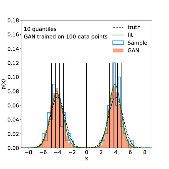
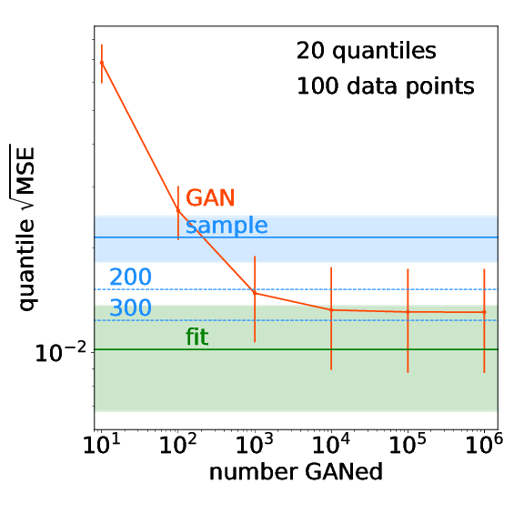
An interesting question for neural networks in general, and generative networks in particular, is how much physics information the networks include in addition to the information in a statistically limited training sample. While a naive answer might be that all the physics a neural network can extract has to be encoded in the training data, the network setup adds information. For instance, it represents smooth functions up to a certain resolution. The question then becomes how much this very basic assumption accounts for in terms of events we can generate.

A simple, but instructive toy example is a one-dimensional camel back function [31], two Gaussians defined by two means, two widths, and a relative normalization, shown in the left panel of Fig. 1. The $x$-axis is divided into quantiles. For each of them we compute the statistical error in analogy to a $\chi^{2}$-measure and add those in quadrature. In the right panel we show the combined quantile error for the sample and for a 5-parameter fit benchmark. First, we see how the fit has a much smaller quantile error than the original 100-point sample. We can specify the additional information when we compare it to the number of sampled events we would need for the same quantile error. For the 20 quantiles in shown in the right panels of Fig. 1 the fit is worth around 500 events instead of the 100-event sample.

Clearly, a simple generative network will not have this kind of amplification factor above five. Nevertheless, a GAN can be trained and then used to generate up to $10^{6}$ events. We first see that generating more than 10,000 events does not change the quantile error and hence does not add more information. Second, we can read off the amplification factor and find that these 10,000 GANned events are worth almost 300 sampled events. In Ref. [31] the authors show that this kind of behavior extends to sparsely populated and high-dimensional phase space, and that the amplification factor increases with sparseness. The amplification factor of the GAN trails the amplification factor of the fit for the 1-dimensional example. While a quantitative result on achievable amplification factors of generative networks in LHC simulations will depend on many aspects and parameters, this simple result indicates that using generative networks in LHC simulations can lead to an increase in precision.

3 Neural networks in event generators

An obvious application of machine learning at the LHC are event generators. These are the simulation tools which put LHC physics into its unique position when it comes to understanding all aspects of the data and comparing it to first-principles theory predictions. Modules inside the generators describe the hard scattering, jet radiation, and even hadronization essentially from first principles. This means their input is a set of Lagrangians defined at a few distinct energy scales. Finally, the output from the event generators is fed into detector simulations, based on the detailed description of the different sub-detectors. The numerical tool behind this generation chain is Monte Carlo simulations, which means that events are described by a long chain of random numbers which describe the individual steps independently from each other. As we will discuss in detail, modern machine learning offers many ways to improve such simulations. The practical question is where it can significantly speed up or increase the precision of the LHC simulation chain.

1 Phase space integration

One challenge in event generation at the LHC is the balance between global phase space coverage and the precise mapping of narrow local structures. The advantage of the established Monte Carlo methods is that they guarantee full phase space coverage, including regions where the matrix elements are very small. For a given algorithm this global coverage has to be balanced with the local resolution, which means that we have to ensure that the event generator also resolves fine structures like phase space boundaries or intermediate resonance peaks. Algorithms like Vegas [32] employ importance sampling, which means they adapt their grid of phase space points to the structures of the integrand and keep track of the Jacobian in terms of phase space weights. This method is nothing but a coordinate transformation of the phase space such that the Jacobian absorbs the main features of the integrand and the actual integration is now over a flat function. An prime example is the mapping of a Breit–Wigner propagator via

$$\int ds\;\frac{C}{(s-m^{2})^{2}+m^{2}\Gamma^{2}}=\frac{1}{m\Gamma}\int dz\;C\quad\text{with}\quad\tan z=\frac{s-m^{2}}{m\Gamma}\;.$$ (11)

The weak spot of Vegas is that the adaptive phase space grid still has a rectangular form. This can be improved by training a regression network to describe the mapping $s\to z$ such that the Jacobian of this variable transform absorbs the leading functional behavior of the integrand. In this case the new integral will be over a largely constant function. Tools like Tensorflow [33] provide this Jacobian essentially for free. References [34, 35, 36] show how neural network implementations can be used to integrate simple phase space structures extremely efficiently.

Figure 2: Comparison of the target function value with the corresponding approximations from the regression and generative models. Figure from Ref. [34].

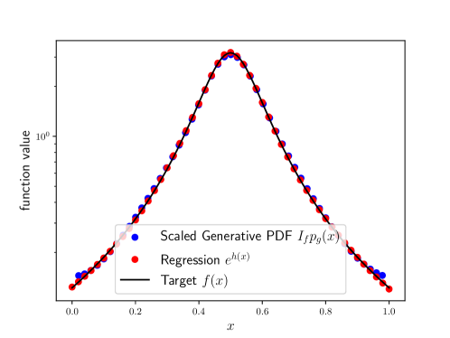
In Ref. [34] the author follows a slightly different approach and apply a generative network to evaluate the phase space integral. This GAN encodes the relation between a known, simple prior distribution and the integrand. In Fig. 2 we show how the regression network and the GAN map out the Breit–Wigner distribution of Eq.(11). For the example of a multi-dimensional camel function the GAN integration outperforms not only Vegas, but also a similar BDT implementation. A state-of-the-art version of a deep-learning integrator is i-flow [22, 37]. It uses a normalizing flow network and coupling layers to optimize the phase space mapping. The limitation of man of these studies is that they focus on phase space integration and not on phase space sampling or event generation. This means that for applications in LHC simulations we have to take the step from regression networks to generative networks discussed in Sec. 2. We will follow up this thought in Sec. 4.

2 Matrix elements

A main ingredient to event simulation is the form of the matrix element. We will discuss the features of matrix element estimation in more detail in Sec. 4 but mention some regression approaches already here. An early attempt of using machine learning on matrix elements targets the partonic process $gg\to ZZ$ [38]. Here the leading order is one loop, which means that the evaluation of the amplitude is significantly slower than the usual tree level calculations. At the same time, the simple $2\to 2$ topology without intermediate resonance leaves us with a low-dimensional phase space and relatively flat distributions. While for the simple $2\to 2$ scattering a BDT is sufficient to encode the matrix element, more complex processes as those discussed below require advance machine learning tools. On the other hand, for instance NNLO calculations are limited by the calculation of loop-induced amplitudes, so this approach appears very promising.

A technically more sophisticated analysis targets the process

$$e^{+}e^{-}\to 3~{}...~{}5~{}\text{jets}$$ (12)

to NLO [39]. For four or five jets in the final state the precise calculation of the matrix element becomes computationally expensive. The question is how it can be encoded in a regression network, mapping the $n$-jet phase space onto the real value of the scattering amplitude. The key parameter is the pair-wise invariant mass of two partons, which diverges in the soft and collinear limits. The regression network features a MSE loss function and is implemented in Keras [40] and Tensorflow [33] with the Adam [41] optimizer.

The actual analysis focuses on a detailed study of the network uncertainties [42], especially in the critical, divergent phase space regions. There the best regression networks achieve a precision of up to 1% in the value of the matrix element squared. As a systematic framework for error analyses, Bayesian networks also discussed in this volume have been applied to jet regression [43] and jet classification [44]. These analyses indicate that the framework can be applied in particle physics with its conservative frequentist approach. A detailed comparison to the ensemble approach proposed in Ref. [39] could be a natural next step.

Figure 3: Comparison of true and GANned $pp\to\ell^{+}\ell^{-}$ events for the input samples and the GAN-subtracted sample. The right panels include the error envelope propagated from the input statistics. Figure from Ref. [45].

Divergent phase space regions and their regularization with the help of subtraction terms are a known numerical challenge in LHC simulations. They can be treated with a subtraction GAN [45]. The task is to start with two different event samples and train a GAN such that its output follows a probability distribution given by the difference of the two training samples. In one dimension this could be a base distribution $P_{B}$ and a subtraction distribution $P_{S}$

$$P_{B}(x)=\frac{1}{x}+0.1\qquad\text{and}\qquad P_{S}(x)=\frac{1}{x}\;.$$ (13)

such that the GANned events follow the constant target distribution

$$P_{B-S}=0.1\;.$$ (14)

In Ref. [45] this toy example is expanded to collinear subtraction with Catani–Seymour kernels, similar to the FKS subtraction used in Ref. [39]. The main difference between these two studies is that the former trains a generative network.

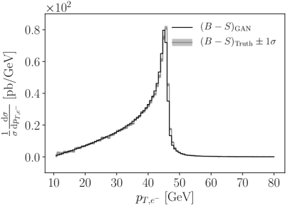
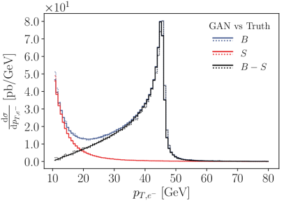
An alternative use for the subtraction GAN are studies of LHC signal processes. For instance, the kinematic distributions of Higgs decays to four fermions reflect the tensor structure of the Higgs coupling to gauge bosons. In traditional methods we start from a combined sample of signal and background events and subtract the background events using some kind of naive or advanced side band analysis [46]. A subtraction GAN could be trained on the measured signal-plus-background sample and an appropriately prepared background sample and then produce signal events with all correlations. In Fig. 3 we show results for the simple example

$$B:\qquad pp \to\ell^{+}\ell^{-}$$

$$S:\qquad pp \to\gamma\to\ell^{+}\ell^{-}\;,$$ (15)

such that $B-S$ gives the $Z$-induced contribution including the interference term. The GAN setup follows Ref. [5], discussed in Sec. 3. In passing, it also illustrates how GANs can surpass statistical limitations from the input samples, as we can see in the right panels of Fig. 3. While the error envelope of the binned subtraction are given by the statistical uncertainty of the two original samples, the smaller variation of the GANned prediction benefits from the combined subtraction and interpolation.

3 Parton shower

The second step in an LHC event simulation is typically the treatment of jet radiation. It is also described by first-principles QCD, if we account for large soft and collinear logarithms [47]. The problems in describing it with a generative network are that it includes a very large number of particles in the final state, that it covers a wide range of energies, and that the self-similar structure of collinearly enhanced radiation needs to be accommodated. Eventually, there will be fully functional GAN showers for LHC analyses [48], but at this stage we only discuss some early applications of neural networks in parton showers.

Figure 4: Comparison between the 500 most signal- or $W$-looking (left) and most background- or QCD-looking (right) jet images, from the truth set (top) and the GANned set (bottom). Figure from Ref. [49].

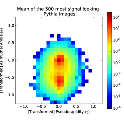
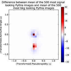
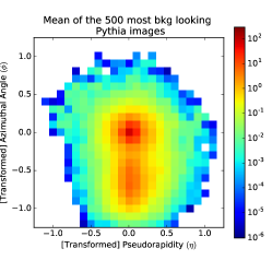
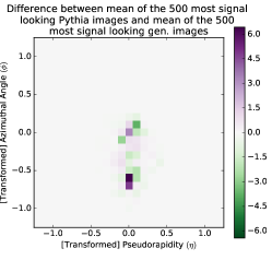
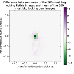
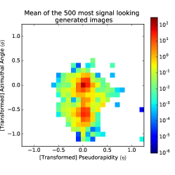
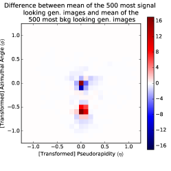
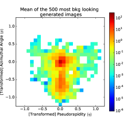
A standard way of representing jets in machine learning is jet images, 2-dimensional pixelized images of the calorimeter output in the rapidity vs azimuthal angle plane. Such images can be GANned using standard machine learning techniques, for instance loss functions which combine fake vs truth discrimination with QCD vs $W$-decay discrimination [49]. The training data for this jet image GAN are large-size Pythia8 [1] jets from QCD or from hadronic $W$-decays. They are required to be in the narrow range $p_{T}=250~{}...~{}300$ GeV, to define a homogeneous sample. In addition, the jet images undergo basic pre-processing such that the hardest constituent is in the center and the second-hardest constituent is rotated to point down. The standard GAN setup is complemented by the additional class information about whether the jet comes from QCD or from $W$-decays. Because it operates on jet images, the network includes a set of convolutional layers, similar to the usual jet classification networks. It is implemented with Keras [40] and Tensorflow [33] and uses the Adam [41] optimizer.

A detailed study of the generated jets shows that they show promise in reproducing the relevant high-level observables like jet mass and subjettiness sample-wise. An interesting way of testing if the GAN has learned the correct patterns is to train a classification network on truth or on GANned samples and then test this network on truth or GANned jets. It turns out that the GANned jets work well as a training sample, apparently too well, suggesting that the GAN has difficulties generating jets in the grey zone between typical QCD and typical $W$-decay jets. In Fig. 4 we show a detailed comparison of the 500 most signal-like and 500 most-background like jets out of 200k truth and GANned jets each. The 2-dimensional histograms for the difference have a linear heat map. For these jets the network reproduces the QCD and $W$-decay patterns faithfully, and some of the apparent differences are explained by bin migration.

Another early application of machine learning to parton showers [37] uses a regression network to apply an a-posteriori reweighting to a parton shower. An example are the reference value and the scale choice of $\alpha_{s}(\mu_{R}^{2})$, which enters the parton shower in a non-trivial way. Varying these two parameters allows us to include theory uncertainties in an analysis of parton showers. The study finds that even a relatively simple network predicts the re-weighting factors for different observables with a precision of better than 2% with a promising gain in speed.

Figure 5: Comparison of true and generated jets in terms of the number of activated pixels per image, the reconstructed soft-drop multiplicity, and the jet mass from the modified Mass Drop Tagger. Figure from Ref. [6].

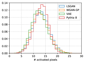
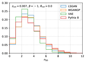
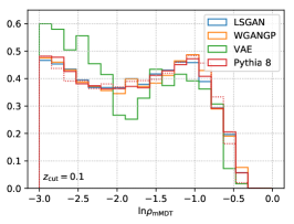
Our last example for using neural networks on parton showers generates Lund plane images using a GAN [6]. The starting points are large jets with $p_{T}>500$ GeV generated with Pythia8 [1] and then passed through the fast detector simulation Delphes [50]. Each jet is then encoded through its clustering history in a sparsely populated 2-dimensional image of the $R$-separation and the relative transverse momentum. This 2-dimensional representation is different from the usual jet images, which are defined as sparsely scattered pixels encoding the energy measured in calorimeter cells. The usual jet images encoding the calorimeter or even particle flow output define a starting point whenever we want to use machine learning on low-level observables. In contrast, Lund plane images represent the high-level output of a jet algorithm. They images are grouped into batches of 32 and used as training input to a least-square GAN, a gradient-penalty WGAN, and a VAE. The GANs employ a set of 2-dimensional kernels. In Fig. 5 we compare the generated showers with the truth information in terms of different observables. While the two GANs lead to comparable results, the VAE performs visibly worse. Of the two GANs the LS version performs better when generating individual sparse Lund images rather than distributions over batches. At this stage it is still too early to speculate what the optimal architecture for Lund plan images will be.

4 SHERPA and normalizing flows

The authors of the event generator Sherpa [51] have published two studies on how the phase space sampling could be improved using deep learning. Both of them use normalizing flows with their invertible coupling layers. The authors of Ref. [21] start from the architecture of the i-flow integrator [22], implement it in Sherpa, and study the LHC process

$$pp\to W/Z+n~{}\text{jets}\;.$$ (16)

The neural network replaces the Vegas-like importance sampling. Its task is to re-write an $x$-integration of a function $f(x)$ into a new variable $x^{\prime}$ such that the combination of the original integrand with the Jacobian, $w=f(x^{\prime})/J$, is as close to a constant value over phase space as possible. All other parts of the Sherpa integration, including the multi-channel structure, remain the same. This implies that the sampling is still guaranteed to cover the full phase space. We recall that a standard generative network evaluates phase space following the training events, without any guaranteed coverage. Any improvement in constructing a phase space mapping by multi-dimensional interpolation should be visible in the unweighting efficiency of the phase space points. This efficiency can be estimated by the ratio of the average to the maximum event weights $\langle w\rangle/w_{\text{max}}$, where the size of the denominator can be limited by evaluating it in batches.

Unweighting efficiencies for the standard Sherpa integration and the normalizing flow network. Table slightly modified from Ref. [21]. unweighting efficiency LO QCD NLO QCD (RS) $\langle w\rangle/w_{\rm max}$ $n=$0 $n=$1 $n=$2 $n=$3 $n=$4 $n=$0 $n=$1 $W^{+}\text{$+n$ jets}$ Sherpa $3\cdot 10^{-1}$ $4\cdot 10^{-2}$ $8\cdot 10^{-3}$ $2\cdot 10^{-3}$ $8\cdot 10^{-4}$ $1\cdot 10^{-1}$ $5\cdot 10^{-3}$ NN+NF $6\cdot 10^{-1}$ $1\cdot 10^{-1}$ $1\cdot 10^{-3}$ $2\cdot 10^{-3}$ $9\cdot 10^{-4}$ $1\cdot 10^{-1}$ $4\cdot 10^{-3}$ Gain 2.2 3.3 1.4 1.2 1.1 1.6 0.91 $W^{-}\text{$+n$ jets}$ Sherpa $3\cdot 10^{-1}$ $4\cdot 10^{-2}$ $8\cdot 10^{-3}$ $2\cdot 10^{-3}$ $1\cdot 10^{-3}$ $1\cdot 10^{-1}$ $5\cdot 10^{-3}$ NN+NF $7\cdot 10^{-1}$ $2\cdot 10^{-1}$ $1\cdot 10^{-2}$ $2\cdot 10^{-3}$ $8\cdot 10^{-4}$ $2\cdot 10^{-1}$ $4\cdot 10^{-3}$ Gain 2.4 3.3 1.4 1.1 0.82 1.5 0.91 $Z\text{$+n$ jets}$ Sherpa $3\cdot 10^{-1}$ $4\cdot 10^{-2}$ $2\cdot 10^{-2}$ $5\cdot 10^{-3}$ $1\cdot 10^{-1}$ $5\cdot 10^{-3}$ NN+NF $4\cdot 10^{-1}$ $1\cdot 10^{-1}$ $1\cdot 10^{-2}$ $2\cdot 10^{-3}$ $2\cdot 10^{-3}$ $6\cdot 10^{-3}$ Gain 1.2 2.9 0.91 0.51 1.5 1.1

In Tab. 4 we show the comparison of unweighting efficiencies with the standard Sherpa integrator and the i-flow network. It uses narrow jets with $p_{T}>20$ GeV and $|\eta|<6$, so a relatively large number of jets is expected in a typical LHC event, challenging the event generation. The gain in unweighting efficiency is clearly visible for the first two jets. Beyond this the flow network gains little, which contradicts the naive expectation based on an improved neural network interpretation for high-dimensional phase spaces. Instead, there seems to be a limiting factor to the performance of the flow network, which might have to do with the fact that all other parts of the generator, including the multi-channeling, are kept the same.

A second Sherpa study [23] also uses a normalizing flow network to replace the importance sampling module, but with a slightly different setup of the coupling layers. It studies the reference process

$$pp\to n~{}\text{gluons}\;,$$ (17)

also with small jets and $p_{T}>30$ GeV. Here we know that the QCD (antenna) radiation pattern defines up to 120 Feynman diagram topologies or channels, which can be mapped onto three independent channels for $n=4$. The analysis of the unweighting efficiencies confirms the bottom line of Ref. [21], namely that there is an improvement visible for $n=3$, but not anymore for $n=4$. This apparent breakdown is unexpected and needs more detailed studies.

Figure 6: Comparison of events from classic and flow network importance sampling in terms of $p_{T}$ of the leading three jets (for up to four jets). The middle panes compare the Monte Carlo errors, the lower panes show the mean event weights per bin. Figure from Ref. [23].

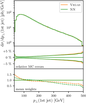
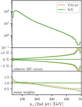
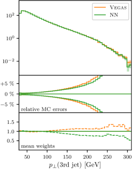
In Fig. 6 we show a physics result from this study, namely the spectra of the three leading jets for $n=4$. In the top panels we see that the two importance sampling approaches, Vegas and flow networks, both produce consistent results. Below, we see that also the MC uncertainty for the two approaches are consistent and remain below 2% as long as we stay away from the tails. Finally, in the bottom panes we show the mean weights $w=f/J$ introduced above. The perfect importance sampling would lead to a flat $w$-distribution over phase space, in this case unity everywhere. For the two leading jets both methods sample the tail too often, filling the histogram with many events of smaller weight. For the third jet Vegas starts to under-populate the tail while the flow network maintains the pattern from the leading two jets.

An interesting aspect of this application of normalizing flows is that it does not use the invertible nature of the coupling layers. Instead, it benefits from the easy calculation of the derivative of the Jacobian. The integrator networks are similar to other generative networks in the sense that they map a random number input to phase space events. They do, however, produce weighted events, which by unfolding can be turned into unweighted events the same way they are produced by other generative networks.

4 GANs and VAEs as event generators

In simulating LHC events increased precision comes at a high price in computing. Leading order calculations are typically cheap, but can really only be considered order-of-magnitude estimates; NLO-QCD predictions have meaningful theory errors anywhere in the 20% to 50% range and are available through automized tools [52, 51]; precision analyses require NNLO or even N³LO in QCD and often require a wealth of numerical tricks to be used in LHC analyses, some of them involving machine learning, as discussed in Sec. 2. An alternative way of employing machine learning beyond improving generators is to train generative networks on any combination of simulated and actual events and then use their ability to learn and interpolate phase space structures to simulate large reference samples. We describe recent developments in this direction for three benchmark processes: the Drell-Yan process, multi-jet production, and top pair production at the LHC.

1 $Z\to\ell\ell$ production

The, arguably, best-studied standard candle at the LHC is the Drell-Yan process

$$pp\to\ell^{+}\ell^{-}\;+\text{jets},$$ (18)

where $\ell$ symbolizes visible leptons as well as invisible neutrinos, the latter being the leading background to dark matter searches.

In Ref. [53] the authors design a GAN to generate these events, described by the 4-vectors of the, in that case, two muons and up to five jets. In Sec. 3 we saw that for a sufficiently large number of jets this process is indeed a challenge and standard benchmark for Monte Carlo generators. The network is trained on Pythia8 [1] events including the fast detector simulation Delphes [50] and a pile-up rate of 20 collisions on average. This simulation defines additional observable features which are evaluated for the network training, namely the number of primary vertices, the detector-induced missing transverse momentum vector, and the muon isolation.

Figure 7: Comparison of true and GANned $pp\to\ell^{+}\ell^{-}$ events in terms of standard kinematic distributions. Figure from Ref. [53].

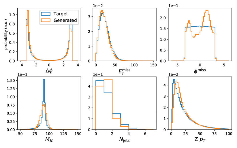
The GAN employed for this paper includes a regression loss involving one process-specific feature, namely the position and the width of the $Z$-peak, in addition to the binary cross entropy

$$L=L_{\text{BCE}}+\lambda_{m}\left(m_{Z}-m_{\ell\ell}\right)^{2}+\lambda_{\sigma}\left(\sigma_{Z}-\sigma_{\ell\ell}\right)^{2}\;,$$ (19)

with $\lambda_{m}=\lambda_{\sigma}=10^{-4}$. The width $\sigma_{Z}=7.7$ GeV is given by the detector simulation. The network is implemented in Keras [40] with a Tensorflow [33] back-end, with a LeakyReLU activation. The comparison of the $Z$-mass and width goes beyond individual events and uses an event batch produced by the generator.

The quality of the GANned events can be tested with a list of kinematic observables, including the invariant mass of the two leptons and the number of jets with $p_{T}>15$ GeV. The corresponding distributions are shown in Fig. 7. Removing the two $Z$-related terms from Eq.(19) has a negligible effect on the muon momenta and on their central invariant mass, but leads to an over-estimate of the detector-level $Z$-width by almost a factor of two. We will come back to such intermediate mass peaks in Sec. 3. The only other class of problematic observables are the transverse jet momenta, because of the combination of the actual spectra and the peak from zero-padding events with fewer jets. Nevertheless, in the lower center panel of Fig. 7 we see that the number of jets above threshold is reproduced reasonably well at least up to three jets.

Figure 8: Comparison of the $E_{T}^{\text{miss}}$ distribution for true and GANned $pp\to\ell^{+}\ell^{-}$ events in the low-pileup and high-pileup regime. Figure from Ref. [53].

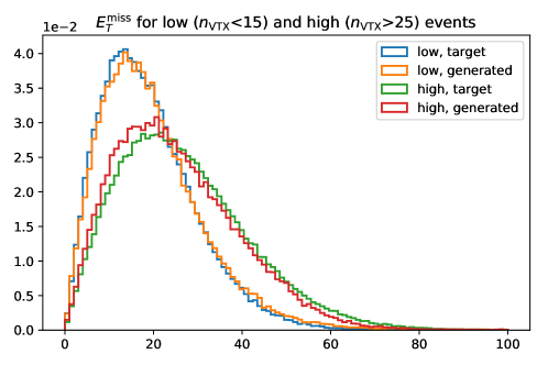
An especially interesting aspect of Ref. [53] is the effect of pile-up, also studied in Ref. [54]. In Fig. 8 we show the missing transverse energy for two subsets of events, with low and high number of pile-up vertices. This application is an example for networks not enforcing energy-momentum conservation, which increases the dimensionality of phase space but allows for detector smearing. As we can see, the GAN reproduces the correlation between the number of pile-up vertices and the smearing of the detector-induced missing energy very well.

A similar physics process, but at an electron-positron collider

$$e^{+}e^{-}\to Z\to\ell^{+}\ell^{-}$$ (20)

is the starting point of Ref. [14]. The authors train on combined MG5aMCNLO samples [52] for $\ell=e,\mu$, where depending on the lepton flavor one set of 4-momenta is always set to zero. This setup increases the dimensionality of the final state from eight to 16. Because the simulation does not include detector effects, the $m_{\ell\ell}$ distribution now has a Breit-Wigner shape with the physics $Z$-width. This simulation also does not include any explicit information on the intermediate particle in the loss function.

The generative network employed here is a modification of a VAE based on a combination of MSE and KL-divergence, as mentioned in Sec. 2. The so-called B-VAE developed for this purpose buffers density information in the latent space and is implemented with Keras [40], Tensorflow [33] and cuDNN [55].

Figure 9: Comparison of $e^{+}e^{-}\to\ell^{+}\ell^{-}$ events for the truth, a VAE with a standard normal prior (blue) and the B-VAE (red). Figure from Ref. [14].

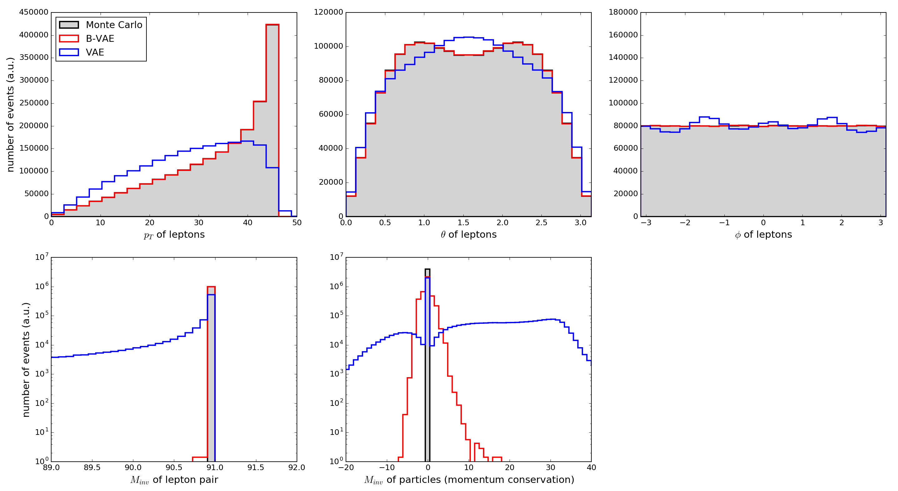
In Fig. 9 we show the corresponding kinematic distributions and confirm that unlike a naive VAE the B-VAE reproduces all of them. The last panel shows the invariant masses of the leptons, which should be zero and is now spread because the network learns the components of the external 4-vectors without the mass constraint. This observed smearing reflects a problem of generative networks, namely that they are not good at learning constant numbers [56]. The reason is that the combination of generator and discriminator updates will constantly force the two networks to move within a typical phase space distance and generate a noisy distribution.

2 Multi-jets

Multi-jet production is the most frequent process at the LHC and affects a huge number of analyses. Depending on the kinematic cuts, the hard process includes at least two hard partons

$$pp\to q\bar{q},gg,qg,\bar{q}g\;,$$ (21)

where these hard partons then generate at least two hard jets. Additional jets can be produced through hard scattering, initial state radiation, or final state radiation. Because of the collinear enhancement and the relatively large strong coupling, most jet events at the LHC have many more than two jets. Simple analyses study, for instance, the relative rate of $n$ and $n+1$ jets, which can be predicted from QCD [47]. The challenges in simulating multi-jet events are, on the one hand, the variable number of jets in the final and, on the other hand, the required precision of a given analysis. The former comes from the fact that we cannot rely on counting powers of the strong coupling in perturbation theory, but have to re-sum large logarithms of jet radiation. The latter means that we have to combine fixed-order calculations with resummed calculation to high precision [47]. An alternative approach to simulating jet backgrounds could be generative networks describing this process based on data rather than theory simulations.

Figure 10: Comparison of true (gray) and GANned (black) multi-jet events including detector effects. Figure from Ref. [57].

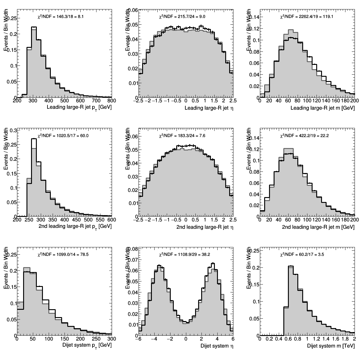
The authors of Ref. [57] train a GAN to simulated LHC events with at least two hard jets. The training data is simulated with MG5aMCNLO [52] and Pythia8 [1]. It relies on Delphes [50] for fast detector simulation and FastJet [58] for jet reconstruction. The large jet size of $R=1.0$ ensures that there are not too many jets in the final state, for example from final state splittings. To enforce hard jets, all events are required to have a scalar sum of all transverse momenta $H_{T}>500$ GeV.

The GAN is implemented in Keras [40] and Tensorflow [33] with the Adam [41] optimizer. All layers except for the last have a LeakyReLU activation function. In the input format the azimuthal angle of the leading jets is set to zero, exploiting a symmetry of the physical system. Another, symmetry is exploited through doubling the training data by reversing the rapidity.

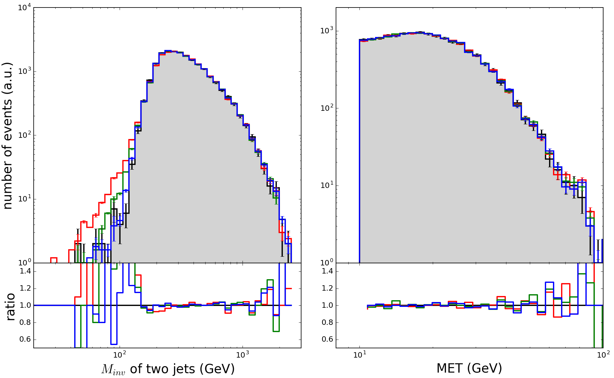
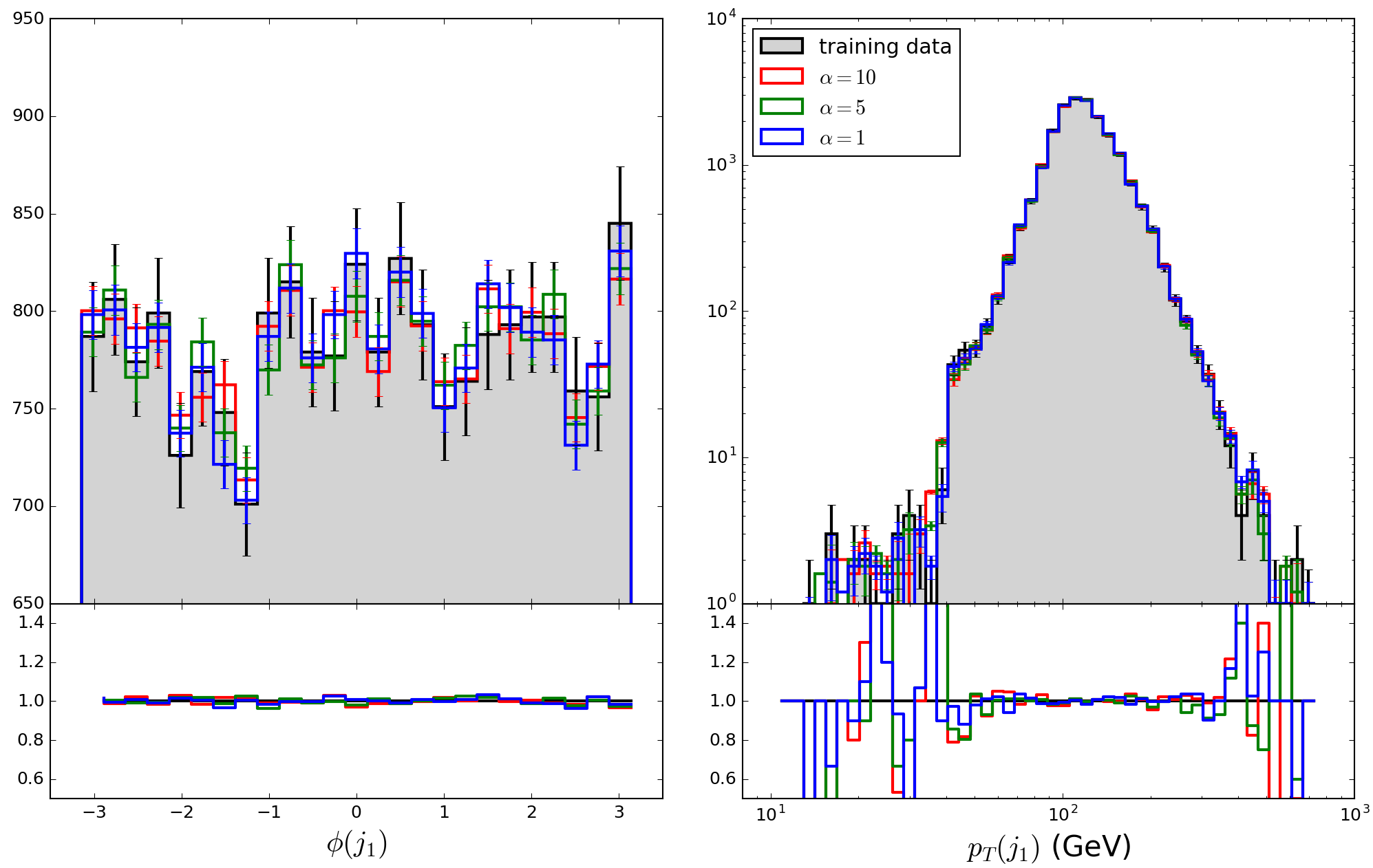
In Fig. 10 we show a set of kinematic distributions for the training events and the generated events. The quoted $\chi^{2}$ value quantifies the agreement between the respective true and GAN distributions. A typical feature of the multi-jet process is that most of the kinematic distributions are flat compared to processes with intermediate mass peaks. The only critical feature, already discussed in Sec. 3, is the sharp phase space boundary for $p_{T}^{\text{min}}$, in this case enforced through a cut on $H_{T}$ and not fully aligned with the shown $p_{T}$. We know that a slight misalignment between a sharp boundary and the input parametrization helps the GAN to model the feature, because it softens the sharp edge. Nevertheless, there remains a slight deviation for instance around the $p_{T}$-threshold of the second-hardest jet. The last row of plots in Fig. 10 shows the kinematic recoil to the leading two jets. This recoil is generated by radiating a variable number of additional jets, so the results illustrate that the multi-jet GAN learns this variable number of jets.

Figure 11: Comparison of true (gray) and GANned (black) multi-jet events without detector effects. The red line shows a 4-parameter function fitted to the training data, including the high-$m_{jj}$ tail. Figure from Ref. [57].

Figure 12: Comparison between experimentally measured truth (gray) and B-VAE results (colored) for the CMS MultiJet primary data set [59]. Figure from Ref. [14].

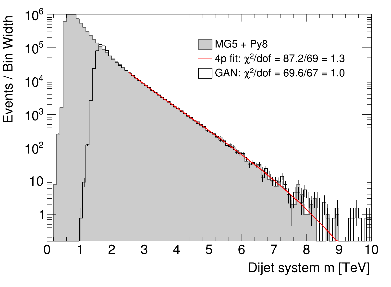
An interesting question lingering in all applications of generative networks is if networks can learn structures not only interpolating between phase space points, but extrapolating into poorly populated regions. For the dijet GAN [57] the authors train their model on a sub-set of the training data with $m_{jj}>1.5$ GeV, This means they focus on the high-mass tail of the distribution and we can ignore issues in the low-mass range. In Fig. 11 we first show the training data, including a 4-parameter fit to the $m_{jj}$ distribution as the baseline description. In addition, we show that the GANned events agree with the training data in the same $m_{jj}$ distribution. The main difference appears for $m_{jj}\gtrsim 8.5$ TeV, where the number of training events becomes small, the fit function exhibits a sharp drop, and the GAN still provides a small number of events.

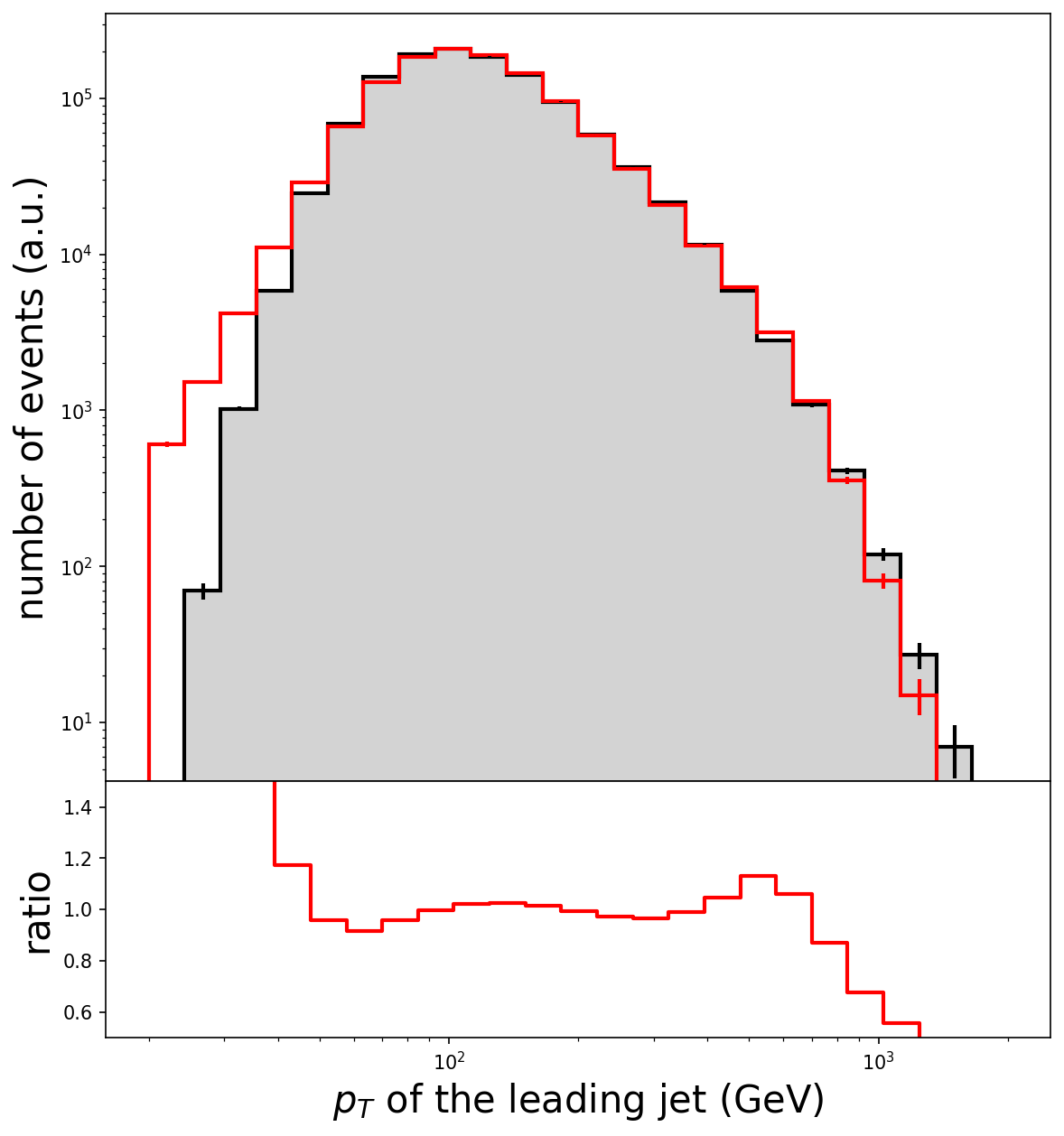
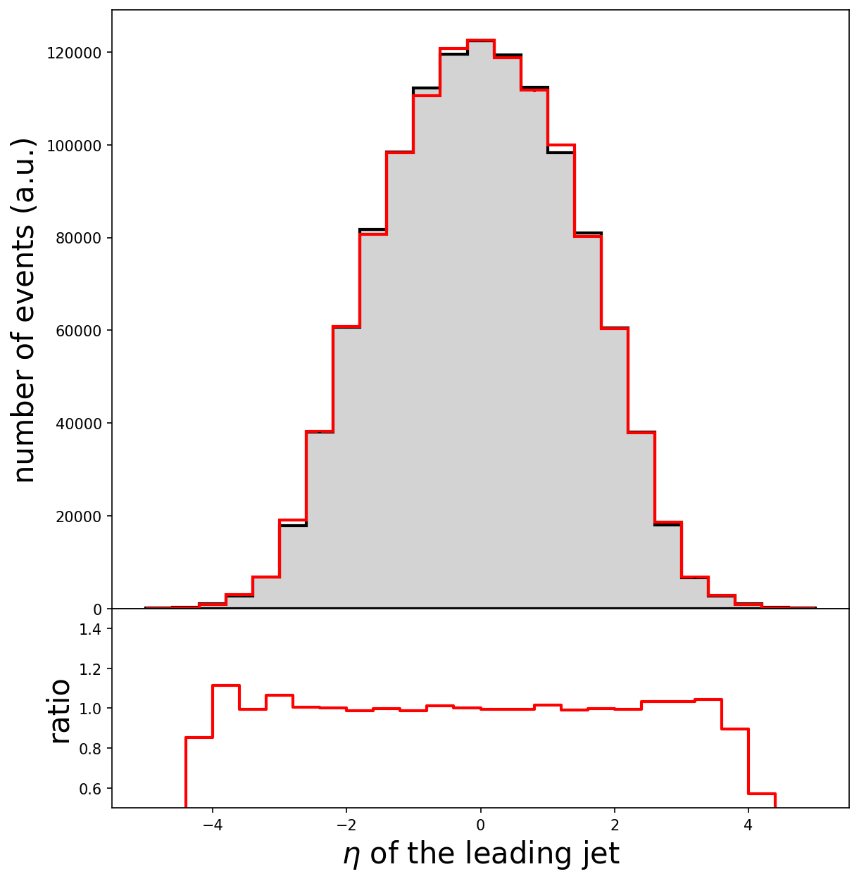
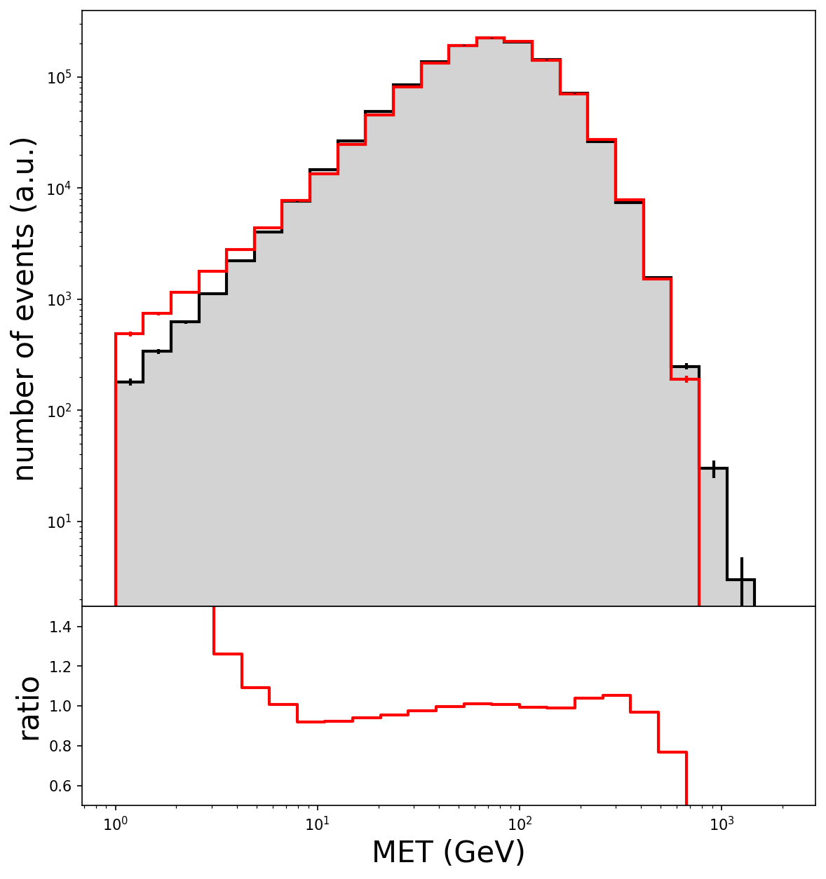
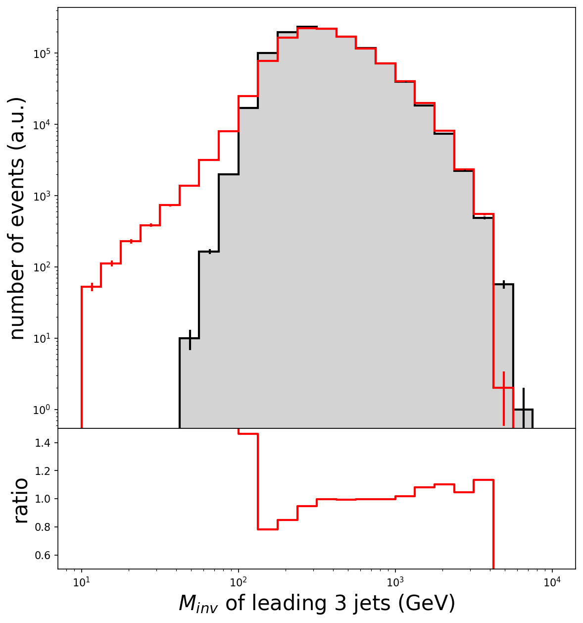
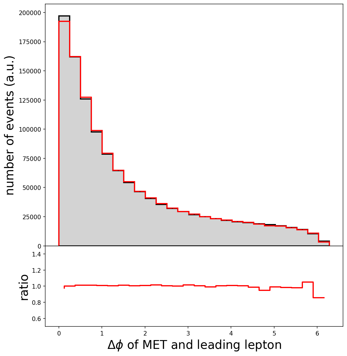
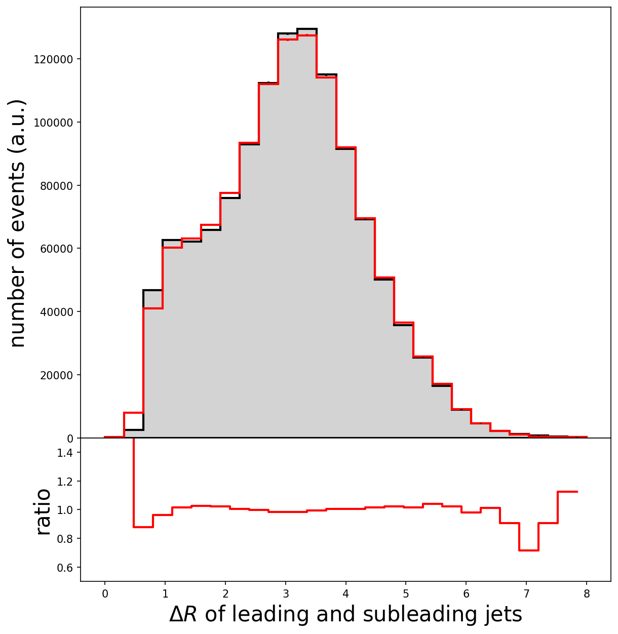
Finally, the B-VAE strategy of Ref. [14] illustrates for multi-jet production how an event sample can be generated from real data as opposed to simulated samples, in this case CMS data from a 7 TeV supersymmetry search [59]. In the original CMS paper this jet sample has been shown to agree with a Pythia8 [1] multi-jet simulation, based on the hard di-jet process. The jet triggers effectively prefer leading jets with $p_{T}\gtrsim$ 100 GeV and a sizeable di-jet mass. Missing transverse energy only appears through detector effects.

The employed B-VAE uses 4-momenta $(E,p_{T},\eta,\phi)$ as input and operates on a 10-dimensional latent space for a variable number of standard jets. In Fig. 12 we show the agreement of the generated events with the original data. In contrast to typical simulated event samples the CMS data does not have sharp phase space boundaries or cliffs in a kinematic distribution. This allows the generative network to, for instance, describe the $m_{jj}$ distribution over essentially the full range.

3 Top pairs

Figure 13: Comparison of true (grey) and VAE (red) events for $t\bar{t}$ production. We show a subset of distributions from Ref. [14].

Top pair production at the LHC,

$$pp\to t\bar{t}$$ (22)

is an especially challenging process because it includes six particles in the final state, out of which we have to construct two intermediate $W$-propagators and two intermediate $t$-propagators.

In Ref. [14] the authors use their B-VAE to describe top pair production with one leptonic top decay. In that case the final state consists of exactly four jets and two leptons. The training data is produced with MG5aMCNLO [52] and supplemented with a fast detector simulation using Delphes3 [50]. The 4-vectors are represented as $(E,p_{T},\eta,\phi)$, defining a 26-dimensional phase space including the two parton-momentum fractions $x$. Hyper-parameters which need to be optimized for the B-VAE include the $B$-parameter weighting the MSE and KL-divergence in the loss function and the dimensionality of the latent space. It is interesting to note that the best-performing models for a set of one- and two-dimensional kinematic distributions in Ref. [14] have an approximately 20-dimensional latent space.

Figure 14: Comparison of true and GANned events. The additional panels give the bin-wise ratio. The third panels show the statistic uncertainty on the number of training events in the tails. Figure from Ref. [5].

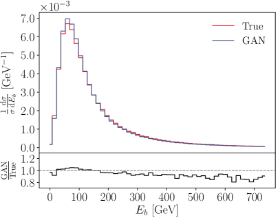
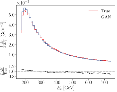
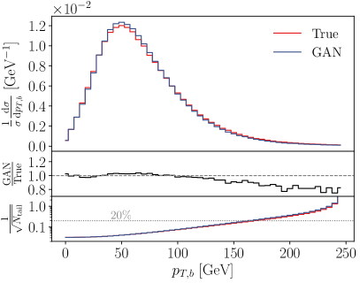
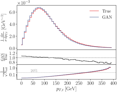
In Fig. 13 we show some of the kinematic distributions, describing the final state particle in the upper row and correlating the final state particles in the lower row. In general, the B-VAE learns the features of the production process. The challenge in the transverse momentum distribution, as compared to the rapidity, is the sharp drop-off for small $p_{T,j}$. Such sharp features or even phase space boundaries are a known and obvious challenge for any generative network [56, 60]. The reason is that the end of such a distribution is described by a very small number of events, so the network will be limited by the training statistics. Good examples for smooth distributions are $\eta_{J,1}$, $\Delta\phi(\ell,\text{MET})$, or $\Delta R(j_{1},j_{2})$ where the precision of the B-VAE is shown to be around 10% at least.

The $t\bar{t}$ study in Ref. [5] focuses on an open question from the results shown in Ref. [14] and an obvious problem found in Ref. [53], namely intermediate on-shell resonances. These narrow phase space features are also a known problem for standard matrix element integrators, which typically employ dedicated coordinate transformations or (multi-channel) phase space mappings. In this case, the training data are top pair events simulated with MG5aMCNLO [52], now decaying into an all-hadronic final state. As a simplification, events with additional jets are not considered. A detector simulation would lead to broader intermediate mass peaks, so it is omitted in reference to the main challenge of the analysis.

The input to the network are the six 4-vectors $(E,p_{x},p_{y},p_{z})$, but with an explicit on-shell condition for each final state particle. They are fed into a GAN with a gradient penalty, implemented in Keras [40] and Tensorflow [33]. The gradient penalty stabilizes the training to a level comparable with a Wasserstein GAN. Some kinematic distributions are shown in Fig. 14, again indicating an agreement with the training data at the 10% level.

Figure 15: Comparison of different kernel functions for the $W$-boson and top mass peaks in the top-pair GAN. Figure from Ref. [5].

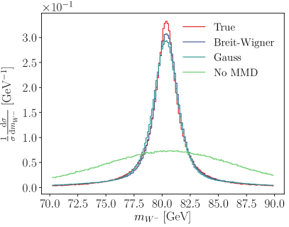
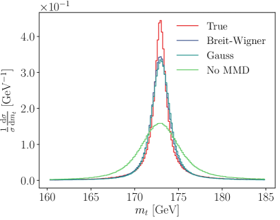
Coming back to the main challenge, invariant masses, like many other narrow phase space features, can be cast into well-defined one-dimensional distributions. In the loss function such a distribution can, for instance, be enforced through a maximum mean discrepancy (MMD) [61], a kernel-based method to compare two samples drawn from different distributions. Using one batch of true data points following a distribution $P_{T}$ and one batch of generated data points following $P_{G}$, it computes a distance between the distributions

$$\text{MMD}^{2}=\big{\langle}k(x,x^{\prime})\big{\rangle}_{x,x^{\prime}\sim P_{T}}+\big{\langle}k(y,y^{\prime})\big{\rangle}_{y,y^{\prime}\sim P_{G}}-2\big{\langle}k(x,y)\big{\rangle}_{x\sim P_{T},y\sim P_{G}}\;,$$ (23)

where $k(x,y)$ can be for instance Gaussian or Breit-Wigner kernels. In both cases the kernel width is a hyperparameter of the network. We show the effect of the different kernels in Fig. 15.

Figure 16: Correlation between $p_{T,t}$ and $p_{T,b}$ for truth (upper left), GAN (upper right), and their relative difference (lower left). We also show $p_{T,b}$ sliced at $p_{T,t}=100\pm 1$ GeV. Figure from Ref. [5].

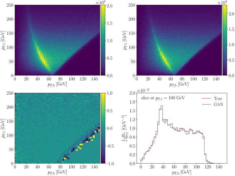
Finally, because not only astronomy lives from nice pictures we also compare a 2-dimensional correlation between the true data and the GAN output in Fig. 16. The correlation between the two transverse momenta includes a Jacobian peak as well as a sharp phase space boundary. The slice in the lower-right panel indicates that the GAN learns the Jacobian peak as well as the sharp boundary with high precision.

5 Inverting the simulation chain

While the LHC simulation chain discussed in Sec. 3 is statistically invertible, it is only ever applied in one direction: we define a physics hypothesis for instance at the hard matrix element level, derive predictions for a data set, and compare with measured data. This procedure turns around our actual physics question, which for instance asks how a kinematic distribution, assuming a hard process, looks for a measured data set. For the interaction between theory and experiment it would therefore be extremely useful, if we could move up and down the simulation chain and compare measurement and theory at any level of data processing.

A simple case would be inverting detector effects, starting from detector-level events and showing parton-level kinematic features. This special case is called unfolding detector effects, and it is an established procedure for one ore two phase space dimensions. Similarly, analyses based on estimating parton-level matrix elements are known as using the matrix element method. The hope is that inverting the LHC simulation chain with machine learning will open new ways to analyze LHC data and compare it to theory predictions without always implementing them into event generators.

1 Parton shower from CycleGANs

When we model an, in principle, invertible simulation like event generation with a neural network, we actually have to decide in which direction we want to apply the network. A intuitive way out is to define a network which maps the incoming data set to the outgoing data set and back. An example is given in Ref. [6], where a CycleGAN turns QCD jets and $W$-decay jets into each other. Alternatively, the same CycleGAN can apply and invert detector effects on a set of jets.

Specifically, the training data are QCD jets and $W$-decay jets from Pythia8 [1], which are passed through Delphes [50]. Each jet is represented by a Lund plane image, introduced in Sec. 3. The mapping of a sample of QCD jets onto a sample of $W$-jets (and vice versa) could help in providing a realistic and large set of fat jets at low simulation cost, similar to the generative networks discussed in Sec. 4. The difference to the other generator models is that it works on a sample of QCD jets, not from scratch. This relieves the network from having to learn the basic structure of a jet and should speed up the generation. On the other hand, a pre-defined structure always bears the danger of introducing a bias into the network.

Figure 17: Top: jet translation from parton-level to detector-level and back. Bottom: corresponding sampled event. Figure from Ref. [6].

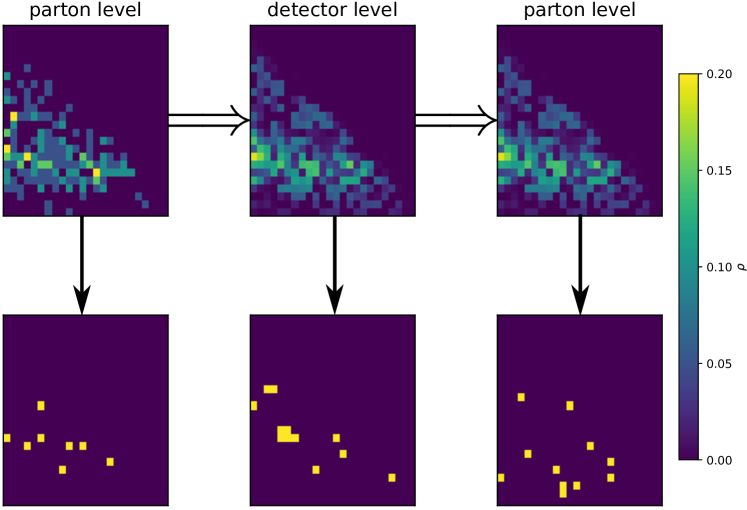
The, arguably, more interesting application is the unfolding of non-perturbative QCD effects and detector effects from a set of observed jets. We show an illustration of this task in the upper panels of Fig. 17. Because Lund images are defined as superpositions of jet batches we sample individual jets from the images at parton level and at detector level. We show individual jets generated from the Lund images in the lower panels of Fig. 17.

A similar approach to unfolding detector effects starting from a good first estimate and then iterating improvement steps has been developed for full LHC events. This Omnifold [62] approach starts with pairs of simulated events at parton level and at detector level, constructs a mapping between simulated and measured detector-level events, and applies this mapping to the parton-level simulations. The output are parton-level events corresponding to measured events, and the procedure is improved through an iteration. This iteration removes a possible bias from the original paired events.

2 Detector unfolding with FCGANs

Using generative networks to directly unfold detector effects from LHC events was first proposed in Ref. [63]. A first, properly generative approach was then established for the process [64]

$$pp\to WZ\to(q\bar{q}^{\prime})\;(\ell^{+}\ell^{-})\;,$$ (24)

trained on Standard Model events generated with MG5aMCNLO [52] and Pythia8 [1]. These parton-level events are then fed through Delphes [50] and FastJet [58] for the jet reconstruction. The analysis does not allow for additional jet radiation, postponing this issue to the analysis discussed in Sec. 3. The task is to train a generative network on a sample of paired parton-level and detector-level events such that the network generates statistically correct parton-level events from a detector-level event. The detector-level event is represented by 4-vectors of high-level analysis objects, like leptons and jets. This detector unfolding has two shortcomings: first, it is only defined statistically in the sense that it does not produce a probability distribution in parton-level phase space for a given detector-level event. Second, it always assumes an underlying physics hypothesis, in our case the Standard Model describing the hard scattering in the training data.

Figure 18: Comparison of parton-level truth and FCGANned distributions for the process $pp\to WZ\to q\bar{q}\,\ell\ell$. The network is trained on the Standard Model and used to unfold events with an injection of $10\%$ $W^{\prime}$ events with $m_{W^{\prime}}=1.3$ TeV. Figure from Ref. [64].

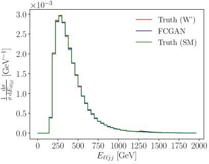
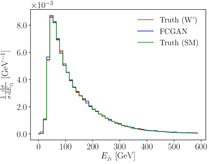
As long as the network is applied to detector-level events which are essentially identical to the training data, the naive GAN approach following Ref.  [63] will work fine. Its architecture follows the event generation GAN in Sec. 3. A problem appears if the test and training data sets are not quite identical. Because the unfolding GAN does not have a notion of similarity in terms of event kinematics, for instance in terms of a latent space metric, it will fail [64]. A way out is to replace the GAN with a fully conditional FCGAN, trained to reproduce a parton-level event only from random noise under the condition of the matching detector-level event with all its physics information. We show the results form this FCGAN in Fig. 18, applied to test data including an irreducible resonance contribution

$$pp\to W^{\prime}\to WZ\to(q\bar{q}^{\prime})\;(\ell^{+}\ell^{-})\;.$$ (25)

While the network does not reproduce the $W^{\prime}$-width correctly, it clearly shows the mass peak which did not exist in the training data. This serves as an indication that it is possible to unfold detector-level events with a controllable model dependence and hence to apply this technique to new physics searches.

3 Hard process from cINNs

Figure 19: Left: illustration of the statistical interpretation of unfolded events for one event. Right: calibration curves for $p_{T,q_{1}}$ extracted from a conditional GAN, a noise-extended eINN, and a conditional cINN. Figure from Ref. [30].

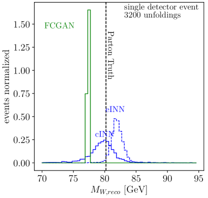
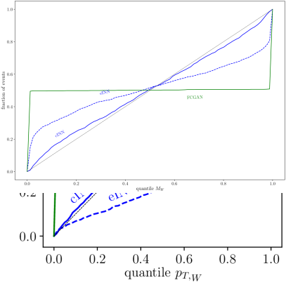
An alternative approach to inverting detector effects is the use of invertible networks [30]. The INN can be trained in the well-defined Delphes [50] direction, mapping parton to detector-level events, and evaluated in the inverse direction to unfold the detector-level distribution. If parton-level and detector-level events live in phase spaces with different dimensions, the smaller representation is extended with noise parameters. Since our task is to construct a non-deterministic mapping, we can try to include more random numbers into the network input and output. Finally, we will use a generative network that includes the foundation of statistical sampling already in the loss function.

The system is benchmarked on the same detector unfolding problem as in Sec. 2 and focus on the statistical interpretation. In the left panel of Fig. 19 we show the distribution in the unfolded parton-level phase space, specifically $p_{T,q_{1}}$ for 3200 independent unfoldings of the same pair of parton-level and detector-level events. First, the FCGAN approach does not allow for a statistical interpretation of the results. While the FCGANned events reproduce the correct kinematic distributions at the parton level, it is not possible to invert a single detector-level event and obtain something like a posterior probability distribution. After padding the standard INN input vectors with a sufficiently large number of random numbers, the so-defined noise-extended eINN does produce a reasonably distribution in parton-level phase space. We can test the width of this distribution through a calibration test: for the right panel of Fig. 19 1500 pairs of parton-level and detector-level events are unfolded 60 times each. For each of them we can look at the position of the parton-level truth in the unfolded distribution, expecting 10% of the 1500 event to lie within the 10% quantile from the left, 20% in the 20% quantile, etc. In the left panel of Fig. 19 we see, however, that the eINN distribution is too narrow to cover the truth. In the right panel we confirm this shortcoming in that the eINN output need re-calibration.

Figure 20: Comparison of parton-level truth and cINNed distributions for the process $pp\to\to(q\bar{q}^{\prime})\;(\ell^{+}\ell^{-})\text{+jets}$. The network is trained on detector-level events with two to four jets. The parton-level events are stacked by number of jets at detector level. Figure from Ref. [30].

We already know that for a statistically sound approach we can try a conditional (invertible) network. As for the FCGAN the direct mapping between parton level and detector level is replaced by a conditioned mapping between parton-level observables and a random variable of the same dimension. Also in Fig. 19 we show the results from this cINN and find that it provides posterior probability distributions with an almost perfect calibration. Modulo an unavoidable model dependence, these studies show that it is possible to compute probability distributions over parton-level phase space for single detector-level events.

An additional benefit of the cINN is that the detector-level input can be of arbitrary dimension. Technically, this makes it possible to unfold events with any number of additional jets [30],

$$pp\to WZ\text{+jets}\to(q\bar{q}^{\prime})\;(\ell^{+}\ell^{-})\text{+jets}\;.$$ (26)

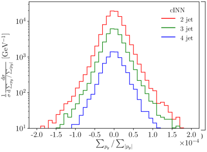
The number of jets in the hard process has to be defined as part of the unfolding model. This flexibility is crucial to include perturbative QCD corrections in the parton-level theory prediction. The stacked $p_{T,q_{1}}$ distribution in Fig. 20 shows how the network unfolds 2-jet, 3-jet, and 4-jet events with similar precision. In the right panel we see that at all unfolded events respect transverse momentum conservation at the level of the hard $2\to 2$ process. Going back to the topic of the review, this last example shows that we cannot just generate events using neural networks, but that we can also invert the generation chain for the LHC. This is a very significant advantage over the usual simulation methods as it allows for completely new ways to compare theory predictions and measured data for future LHC runs.

6 Outlook

We have discussed the application of generative neural networks to event generation for example at the LHC. In the standard approach this is done with Monte Carlo simulations which use Lagrangians as inputs and provide simulated LHC events based on first principles. This approach guarantees full phase space coverage, but it is becoming speed-limited and cannot be inverted in practice. This implies that analyses can only be done at the end of the simulation chain.

We have discussed many ideas to improve and complement this simulation chain using neural networks. In Sec. 3 we have shown how neural networks can be used as modules in contemporary event generators, from phase space simulation to matrix elements and parton showers. Next, we discussed in Sec. 4 how this event generation chain might be replaced by generative networks. We note that this does not imply that neural networks will replace first-principle generators, because only first-principle generators allow us to compare LHC data to complete theory predictions. Instead, event generation networks could be used to increase the number of simulated events or to cover statistical weaknesses of standard simulators for instance in the bulk of high-precision simulations.

Finally, we have discussed how neural networks can invert the simulation chain for the LHC. Such an inversion is at the heart of approaches like the matrix element method. Moreover, a systematic unfolding would enable analyses at any level of the LHC simulation chain and give the experiments access to many more precision predictions. These applications of machine learning to LHC simulations are still at the very beginning, and many conceptual problems are unsolved. For instance, it is not clear how many events a trained network can generate before it is limited by the limited size of the training data, and we do not know how to assign error bars to event samples generated by neural networks. On the other hand, the existing studies clearly indicate the potential of neural networks as part of simulation tools, and there is no doubt that LHC simulations and simulation-based analyses during the upcoming runs will significantly benefit from generative networks.

Acknowledgments

We would like to thank all of our collaborators and discussion partners on generative networks, including Lyonton Ardizzone, Marco Bellagente, Sascha Diefenbacher, Gregor Kasieczka, Ulli Köthe, Ben Nachman, Armand Rousselot, and especially Ramon Winterhalder. We are also grateful to David Rousseau, Paolo Calafiura, and Kazuhiro Terao for giving us this opportunity. Our research is supported by the Deutsche Forschungsgemeinschaft (DFG, German Research Foundation) under grant 396021762 — TRR 257 Particle Physics Phenomenology after the Higgs Discovery.

References

- [1] T. Sjöstrand, S. Ask, J. R. Christiansen, R. Corke, N. Desai, P. Ilten, S. Mrenna, S. Prestel, C. O. Rasmussen, and P. Z. Skands, An Introduction to PYTHIA 8.2, Comput. Phys. Commun. 191 (2015) 159, arXiv:1410.3012 [hep-ph].
- [2] J. Bellm et al., Herwig 7.2 release note, Eur. Phys. J. C 80 (2020) 5, 452, arXiv:1912.06509 [hep-ph].
- [3] S. Höche and S. Prestel, Triple collinear emissions in parton showers, Phys. Rev. D 96 (2017) 7, 074017, arXiv:1705.00742 [hep-ph].
- [4] J. Alwall et al., The automated computation of tree-level and next-to-leading order differential cross sections, and their matching to parton shower simulations, JHEP 07 (2014) 079, arXiv:1405.0301 [hep-ph].
- [5] A. Butter, T. Plehn, and R. Winterhalder, How to GAN LHC Events, SciPost Phys. 7 (2019) 6, 075, arXiv:1907.03764 [hep-ph].
- [6] S. Carrazza and F. A. Dreyer, Lund jet images from generative and cycle-consistent adversarial networks, Eur. Phys. J. C79 (2019) 11, 979, arXiv:1909.01359 [hep-ph].
- [7] M. Arjovsky, S. Chintala, and L. Bottou, Wasserstein gan, arXiv:1701.07875 [stat.ML].
- [8] I. Gulrajani, F. Ahmed, M. Arjovsky, V. Dumoulin, and A. Courville, Improved training of wasserstein gans, arXiv:1704.00028 [cs.LG].
- [9] L. Mescheder, A. Geiger, and S. Nowozin, Which training methods for gans do actually converge?, arXiv:1801.04406 [cs.LG].
- [10] M. Erdmann, L. Geiger, J. Glombitza, and D. Schmidt, Generating and refining particle detector simulations using the Wasserstein distance in adversarial networks, Comput. Softw. Big Sci. 2 (2018) 1, 4, arXiv:1802.03325 [astro-ph.IM].
- [11] M. Erdmann, J. Glombitza, and T. Quast, Precise simulation of electromagnetic calorimeter showers using a Wasserstein Generative Adversarial Network, Comput. Softw. Big Sci. 3 (2019) 1, 4, arXiv:1807.01954 [physics.ins-det].
- [12] J.-Y. Zhu, T. Park, P. Isola, and A. A. Efros, Unpaired image-to-image translation using cycle-consistent adversarial networks, arXiv:1703.10593 [cs.CV].
- [13] D. P. Kingma and M. Welling, Auto-encoding variational bayes, arXiv:1312.6114 [stat.ML].
- [14] S. Otten, S. Caron, W. de Swart, M. van Beekveld, L. Hendriks, C. van Leeuwen, D. Podareanu, R. Ruiz de Austri, and R. Verheyen, Event Generation and Statistical Sampling for Physics with Deep Generative Models and a Density Information Buffer, arXiv:1901.00875 [hep-ph].
- [15] A. Makhzani, J. Shlens, N. Jaitly, I. Goodfellow, and B. Frey, Adversarial autoencoders, arXiv:1511.05644 [cs.LG].
- [16] A. B. L. Larsen, S. K. Sønderby, H. Larochelle, and O. Winther, Autoencoding beyond pixels using a learned similarity metric, arXiv:1512.09300 [cs.LG].
- [17] D. J. Rezende and S. Mohamed, Variational inference with normalizing flows, arXiv:1505.05770 [stat.ML].
- [18] L. Dinh, D. Krueger, and Y. Bengio, Nice: Non-linear independent components estimation, arXiv:1410.8516 [cs.LG].
- [19] I. Kobyzev, S. Prince, and M. A. Brubaker, Normalizing flows: An introduction and review of current methods, arXiv:1908.09257 [stat.ML].
- [20] T. Müller, B. McWilliams, F. Rousselle, M. Gross, and J. Novák, Neural importance sampling, arXiv:1808.03856 [cs.LG].
- [21] C. Gao, S. Hoeche, J. Isaacson, C. Krause, and H. Schulz, Event Generation with Normalizing Flows, arXiv:2001.10028 [hep-ph].
- [22] C. Gao, J. Isaacson, and C. Krause, i-flow: High-dimensional Integration and Sampling with Normalizing Flows, arXiv:2001.05486 [physics.comp-ph].
- [23] E. Bothmann, T. Janßen, M. Knobbe, T. Schmale, and S. Schumann, Exploring phase space with Neural Importance Sampling, arXiv:2001.05478 [hep-ph].
- [24] L. Dinh, J. Sohl-Dickstein, and S. Bengio, Density estimation using real nvp, arXiv:1605.08803 [cs.LG].
- [25] D. P. Kingma, T. Salimans, R. Jozefowicz, X. Chen, I. Sutskever, and M. Welling, Improving variational inference with inverse autoregressive flow, arXiv:1606.04934 [cs.LG].
- [26] G. Papamakarios, T. Pavlakou, and I. Murray, Masked autoregressive flow for density estimation, arXiv:1705.07057 [stat.ML].
- [27] C.-W. Huang, D. Krueger, A. Lacoste, and A. Courville, Neural autoregressive flows, arXiv:1804.00779 [cs.LG].
- [28] L. Ardizzone, J. Kruse, S. Wirkert, D. Rahner, E. W. Pellegrini, R. S. Klessen, L. Maier-Hein, C. Rother, and U. Köthe, Analyzing inverse problems with invertible neural networks, arXiv:1808.04730 [cs.LG].
- [29] L. Ardizzone, C. Lüth, J. Kruse, C. Rother, and U. Köthe, Guided image generation with conditional invertible neural networks, arXiv:1907.02392 [cs.CV].
- [30] M. Bellagente, A. Butter, G. Kasieczka, T. Plehn, A. Rousselot, and R. Winterhalder, Invertible Networks or Partons to Detector and Back Again, arXiv:2006.06685 [hep-ph].
- [31] A. Butter, S. Diefenbacher, G. Kasieczka, B. Nachman, and T. Plehn, GANplifying Event Samples, arXiv:2008.06545 [hep-ph].
- [32] G. P. Lepage, A new algorithm for adaptive multidimensional integration, Journal of Computational Physics 27 (1978) 2, 192 .
- [33] M. Abadi et al., Tensorflow: A system for large-scale machine learning, CoRR (2016) , arXiv:1605.08695 [cs.DC].
- [34] J. Bendavid, Efficient Monte Carlo Integration Using Boosted Decision Trees and Generative Deep Neural Networks, arXiv:1707.00028 [hep-ph].
- [35] M. D. Klimek and M. Perelstein, Neural Network-Based Approach to Phase Space Integration, arXiv:1810.11509 [hep-ph].
- [36] S. Carrazza and J. M. Cruz-Martinez, VegasFlow: accelerating Monte Carlo simulation across multiple hardware platforms, Comput. Phys. Commun. 254 (2020) 107376, arXiv:2002.12921 [physics.comp-ph].
- [37] E. Bothmann and L. Debbio, Reweighting a parton shower using a neural network: the final-state case, JHEP 01 (2019) 033, arXiv:1808.07802 [hep-ph].
- [38] F. Bishara and M. Montull, (Machine) Learning Amplitudes for Faster Event Generation, arXiv:1912.11055 [hep-ph].
- [39] S. Badger and J. Bullock, Using neural networks for efficient evaluation of high multiplicity scattering amplitudes, arXiv:2002.07516 [hep-ph].
- [40] F. Chollet GitHub repository (2015) .
- [41] D. P. Kingma and J. Ba, Adam: A Method for Stochastic Optimization, arXiv:1412.6980 [cs.LG].
- [42] B. Nachman, A guide for deploying Deep Learning in LHC searches: How to achieve optimality and account for uncertainty, arXiv:1909.03081 [hep-ph].
- [43] G. Kasieczka, M. Luchmann, F. Otterpohl, and T. Plehn, Per-Object Systematics using Deep-Learned Calibration, arXiv:2003.11099 [hep-ph].
- [44] S. Bollweg, M. Haußmann, G. Kasieczka, M. Luchmann, T. Plehn, and J. Thompson, Deep-Learning Jets with Uncertainties and More, SciPost Phys. 8 (2020) 1, 006, arXiv:1904.10004 [hep-ph].
- [45] A. Butter, T. Plehn, and R. Winterhalder, How to GAN Event Subtraction, arXiv:1912.08824 [hep-ph].
- [46] A. Andreassen, I. Feige, C. Frye, and M. D. Schwartz, JUNIPR: a Framework for Unsupervised Machine Learning in Particle Physics, Eur. Phys. J. C79 (2019) 2, 102, arXiv:1804.09720 [hep-ph].
- [47] T. Plehn, Lectures on LHC Physics, vol. 886. 2015.
- [48] C. Sauer, “Towards a Data-Driven Simulation of QCD Radiation with Generative Models utilizing Machine Learning Methods.” Heidelberg thesis, 2019.
- [49] L. de Oliveira, M. Paganini, and B. Nachman, Learning Particle Physics by Example: Location-Aware Generative Adversarial Networks for Physics Synthesis, Comput. Softw. Big Sci. 1 (2017) 1, 4, arXiv:1701.05927 [stat.ML].
- [50] DELPHES 3, J. de Favereau, C. Delaere, P. Demin, A. Giammanco, V. Lemaître, A. Mertens, and M. Selvaggi, DELPHES 3, A modular framework for fast simulation of a generic collider experiment, JHEP 02 (2014) 057, arXiv:1307.6346 [hep-ex].
- [51] Sherpa, E. Bothmann et al., Event Generation with Sherpa 2.2, SciPost Phys. 7 (2019) 3, 034, arXiv:1905.09127 [hep-ph].
- [52] J. Alwall et al., The automated computation of tree-level and next-to-leading order differential cross sections, and their matching to parton shower simulations, JHEP 07 (2014) 079, arXiv:1405.0301 [hep-ph].
- [53] B. Hashemi, N. Amin, K. Datta, D. Olivito, and M. Pierini, LHC analysis-specific datasets with Generative Adversarial Networks, arXiv:1901.05282 [hep-ex].
- [54] J. Arjona Martínez, T. Q. Nguyen, M. Pierini, M. Spiropulu, and J.-R. Vlimant, Particle Generative Adversarial Networks for full-event simulation at the LHC and their application to pileup description, arXiv:1912.02748 [hep-ex].
- [55] S. Chetlur, C. Woolley, P. Vandermersch, J. Cohen, J. Tran, B. Catanzaro, and E. Shelhamer, cudnn: Efficient primitives for deep learning, arXiv:1410.0759 [cs.NE].
- [56] A. Butter, T. Plehn, and R. Winterhalder, How to GAN LHC Events, SciPost Phys. 7 (2019) 075, arXiv:1907.03764 [hep-ph].
- [57] R. Di Sipio, M. Faucci Giannelli, S. Ketabchi Haghighat, and S. Palazzo, DijetGAN: A Generative-Adversarial Network Approach for the Simulation of QCD Dijet Events at the LHC, JHEP 08 (2020) 110, arXiv:1903.02433 [hep-ex].
- [58] M. Cacciari, G. P. Salam, and G. Soyez, FastJet User Manual, Eur. Phys. J. C72 (2012) 1896, arXiv:1111.6097 [hep-ph].
- [59] CMS, S. Chatrchyan et al., Search for supersymmetry with razor variables in pp collisions at =7 TeV, Phys. Rev. D 90 (2014) 11, 112001, arXiv:1405.3961 [hep-ex].
- [60] Y. Alanazi, N. Sato, T. Liu, W. Melnitchouk, M. P. Kuchera, E. Pritchard, M. Robertson, R. Strauss, L. Velasco, and Y. Li, Simulation of electron-proton scattering events by a Feature-Augmented and Transformed Generative Adversarial Network (FAT-GAN), arXiv:2001.11103 [hep-ph].
- [61] A. Gretton, K. M. Borgwardt, M. J. Rasch, B. Schölkopf, and A. J. Smola, A kernel method for the two-sample problem, CoRR (2008) , arXiv:0805.2368 [cs.LG].
- [62] A. Andreassen, P. T. Komiske, E. M. Metodiev, B. Nachman, and J. Thaler, OmniFold: A Method to Simultaneously Unfold All Observables, Phys. Rev. Lett. 124 (2020) 18, 182001, arXiv:1911.09107 [hep-ph].
- [63] K. Datta, D. Kar, and D. Roy, Unfolding with Generative Adversarial Networks, arXiv:1806.00433 [physics.data-an].
- [64] M. Bellagente, A. Butter, G. Kasieczka, T. Plehn, and R. Winterhalder, How to GAN away Detector Effects, arXiv:1912.00477 [hep-ph].