A Unified Evaluation of Two-Candidate Ballot-Polling Election Auditing Methods

Abstract

Counting votes is complex and error-prone. Several statistical methods have been developed to assess election accuracy by manually inspecting randomly selected physical ballots. Two ‘principled’ methods are risk-limiting audits (RLAs) and Bayesian audits (BAs). RLAs use frequentist statistical inference while BAs are based on Bayesian inference. Until recently, the two have been thought of as fundamentally different.

We present results that unify and shed light upon ‘ballot-polling’ RLAs and BAs (which only require the ability to sample uniformly at random from all cast ballot cards) for two-candidate plurality contests, which are building blocks for auditing more complex social choice functions, including some preferential voting systems. We highlight the connections between the methods and explore their performance.

First, building on a previous demonstration of the mathematical equivalence of classical and Bayesian approaches, we show that BAs, suitably calibrated, are risk-limiting. Second, we compare the efficiency of the methods across a wide range of contest sizes and margins, focusing on the distribution of sample sizes required to attain a given risk limit. Third, we outline several ways to improve performance and show how the mathematical equivalence explains the improvements.

1 Introduction

Even if voters verify their ballots and the ballots are kept secure, the counting process is prone to errors from malfunction, human error, and malicious intervention. For this reason, the US National Academy of Sciences [4] and the American Statistical Association have recommended the use of risk-limiting audits to check reported election outcomes.

The simplest audit is a manual recount, which is usually expensive and time-consuming. An alternative is to examine a random sample of the ballots and test the result statistically. Unless the margin is narrow, a sample far smaller than the whole election may suffice. For more efficiency, sampling can be done adaptively: stop when there is strong evidence supporting the reported outcome [7].

Risk-limiting audits (RLAs) have become the audit method recommended for use in the USA. Pilot RLAs have been conducted for more than 50 elections in 14 US states and Denmark since 2008. Some early pilots are discussed in a report from the California Secretary of State to the US Election Assistance Commission. In 2017, the state of Colorado became the first to complete a statewide RLA. The defining feature of RLAs is that, if the reported outcome is incorrect, they have a large, pre-specified minimum probability of discovering this and correcting the outcome. Conversely, if the reported outcome is correct, then they will eventually certify the result. This might require only a small random sample, but the audit may lead to a complete manual tabulation of the votes if the result is very close or if tabulation error was an appreciable fraction of the margin.

RLAs exploit frequentist statistical hypothesis testing. There are by now more than half a dozen different approaches to conducting RLAs [8]. Election audits can also be based on Bayesian inference [6].

With so many methods, it may be hard to understand how they relate to each other, which perform better, which are risk-limiting, etc. Here, we review and compare the statistical properties of existing methods in the simplest case: a two-candidate, first-past-the-post contest with no invalid ballots. This allows us to survey a wide range of methods and more clearly describe the connections and differences between them. Most real elections have more than two candidates, of course. However, the methods designed for this simple context are often adapted for more complex elections by reducing them into pairwise contests (see below for further discussion of this point). Therefore, while we only explore a simple scenario, it sheds light on how the various approaches compare, which may inform future developments in more complex scenarios. There are many other aspects to auditing that matter greatly in practice, we do not attempt to cover all of these but we comment on some below.

For two-candidate, no-invalid-vote contests, we explain the connections and differences among many audit methods, including frequentist and Bayesian approaches. We evaluate their efficiency across a range of election sizes and margins. We also explore some natural extensions and variations of the methods. We ensure that the comparisons are ‘fair’ by numerically calibrating each method to attain a specified risk limit.

We focus on ballot-polling audits, which involve selecting ballots at random from the pool of cast ballots. Each sampled ballot is interpreted manually; those interpretations comprise the audit data. (Ballot-polling audits do not rely on the voting system’s interpretation of ballots, in contrast to comparison audits.)

Paper outline: Section 2 provides context and notation. Section 3 sketches the auditing methods we consider and points out the relationships among them and to other statistical methods. Section 4 explains how we evaluate these methods. Our benchmarking experiments are reported in Section 5. We finish with a discussion and suggestions for future work in Section 6.

2 Context and notation: two-candidate contests

We consider contests between two candidates, where each voter votes for exactly one candidate. The candidate who receives more votes wins. Ties are possible if the number of ballots is even.

Real elections may have invalid votes, for example, ballots marked in favour of both candidates or neither; for multipage ballots, not every ballot paper contains every contest. Here we assume every ballot has a valid vote for one of the two candidates. See Section 6.

Most elections have more than two candidates and can involve complex algorithms (‘social choice functions’) for determining who won. A common tactic for auditing these is to reduce them to a set of pairwise contests such that certifying all of the contests suffices to confirm the reported outcome [3, 1, 8]. These contests can be audited simultaneously using methods designed for two candidates that can accommodate invalid ballots, which most of the methods considered below do. Therefore, the methods we evaluate form the building blocks for many of the more complex methods, so our results are more widely relevant.

We do not consider stratified audits, which account for ballots cast across different locations or by different voting methods within the same election.

2.1 Ballot-polling audits for two-candidate contests

We use the terms ‘ballot’ and ‘ballot card’ interchangeably, even though typical ballots in the US consist of more than one card (and the distinction does matter for workload and for auditing methods). We consider unweighted ballot-polling audits, which require only the ability to sample uniformly at random from all ballot cards.

The sampling is typically sequential. We draw an initial sample and assess the evidence for or against the reported outcome. If there is sufficient evidence that the reported outcome is correct, we stop and ‘certify’ the winner. Otherwise, we inspect more ballots and try again, possibly continuing to a full manual tabulation. At any time, the auditor can chose to conduct a full hand count rather than continue to sample at random. That might occur if the work of continuing the audit is anticipated to be higher than that of a full hand count or if the audit data suggest that the reported outcome is wrong. One reasonable rule is to set a maximum sample size (number of draws, not necessarily the number of distinct ballots) for the audit; if the sample reaches that size but the outcome has not been confirmed, there is a full manual tabulation. The outcome according to that manual tabulation becomes official.

There are many choices to be made, including:

How to assess evidence.

Each stage involves calculating a statistic from the sample. What statistic do we use? This is one key difference amongst auditing methods, see Section 3.

Threshold for evidence.

The decision of whether to certify or keep sampling is done by comparing the statistic to a reference value. Often the value is chosen such that it limits the probability of certifying the outcome if the outcome is wrong, i.e. limits the risk (see below).

Sampling with or without replacement.

Sampling may be done with or without replacement. Sampling without replacement is more efficient; sampling with replacement often yields simpler mathematics. The difference in efficiency is small unless a substantial fraction (e.g. 20% or more) of the ballots are sampled.

Sampling increments.

By how much do we increase the sample size if the current sample does not confirm the outcome? We could enlarge the sample one ballot at a time, but it is usually more efficient to have larger ‘rounds’. The methods described here can accommodate rounds of any size.

We assume that the auditors read votes correctly, which generally requires retrieving the correct ballots and correctly applying legal rules for interpreting voters’ marks.

2.2 Notation

Let $X_{1},X_{2},\dots\in\{0,1\}$ denote the sampled ballots, with $X_{i}=1$ representing a vote in favour of the reported winner and $X_{i}=0$ a vote for the reported loser.

Let $n$ denote the number of (not necessarily distinct) ballots sampled at a given point in the audit, $m$ the maximum sample size (i.e. number of draws) for the audit, and $N$ the total number of cast ballots. We necessarily have $n\leqslant m$ and if sampling without replacement we also have $m\leqslant N$.

Each audit method summarizes the evidence in the sample using a statistic of the form $S_{n}(X_{1},X_{2},\dots,X_{n},n,m,N)$. For brevity, we suppress $n$, $m$ and $N$ in the notation.

Let $Y_{n}=\sum_{i=1}^{n}X_{i}$ be the number of sampled ballots that are in favour of the reported winner. Since the ballots are by assumption exchangeable, the statistics used by most methods can be written in terms of $Y_{n}$.

Let $T$ be the true total number of votes for the winner and $p_{T}=T/N$ the true proportion of such votes. Let $p_{r}$ be the reported proportion of votes for the winner. We do not know $T$ nor $p_{T}$, and it is not guaranteed that $p_{r}\simeq p_{T}$.

For sampling with replacement, conditional on $n$, $Y_{n}$ has a binomial distribution with parameters $n$ and $p_{T}$. For sampling without replacement, conditional on $n$, $Y_{n}$ has a hypergeometric distribution with parameters $n$, $T$ and $N$.

2.3 Risk-limiting audits as hypothesis tests

Risk-limiting audits amount to statistical hypothesis tests. The null hypothesis $H_{0}$ is that the reported winner(s) did not really win. The alternative $H_{1}$ is that the reported winners really won. For a single-winner contest,

$$H_{0}\colon p_{T}\leqslant\tfrac{1}{2},\quad\text{(reported winner is false)}$$

$$H_{1}\colon p_{T}>\tfrac{1}{2}.\quad\text{(reported winner is true)}$$

If we reject $H_{0}$, we certify the election without a full manual tally. The certification rate is the probability of rejecting $H_{0}$. Hypothesis tests are often characterized by their significance level (false positive rate) and power. Both have natural interpretations in the context of election audits by reference to the certification rate. The power is simply the certification rate when $H_{1}$ is true. Higher power reduces the chance of an unnecessary recount. A false positive is a miscertification: rejecting $H_{0}$ when in fact it is true. The probability of miscertification depends on $p_{T}$ and the audit method, and is known as the risk of the method. In a two-candidate plurality contest, the maximum possible risk is typically attained when $p_{T}=\frac{1}{2}$.

For many auditing methods we can find an upper bound on the maximum possible risk, and can also set their evidence threshold such that the risk is limited to a given value. Such an upper bound is referred to as a risk limit, and methods for which this is possible are called risk-limiting. Some methods are explicitly designed to have a convenient mechanism to set such a bound, for example via a formula. We call such methods automatically risk-limiting.

Audits with a sample size limit $m$ become full manual tabulations if they have not stopped after drawing the $m$th ballot. Such a tabulation is assumed to find the correct outcome, so the power of a risk-limiting audit is 1. We use the term ‘power’ informally to refer to the chance the audit stops after drawing $m$ or fewer ballots.

3 Election auditing methods

We describe Bayesian audits in some detail because they provide a mathematical framework for many (but not all) of the other methods. We then describe the other methods, many of which can be viewed as Bayesian audits for a specific choice of the prior distribution. Some of these connections were previously described by [11]. These connections can shed light on the performance or interpretation of the other methods. However, our benchmarking experiments are frequentist, even for the Bayesian audits (for example, we calibrate the methods to limit the risk).

Table 1 lists the methods described here; the parameters of the methods are defined below.

Table 1: Summary of auditing methods. The methods in the first part of the table are benchmarked in this report.

Method	Quantities to set	Automatically risk-limiting
Bayesian	$f(p)$	—
Bayesian (risk-max.)	$f(p),\text{for }p>0.5$	✓
BRAVO	$p_{1}$	✓
MaxBRAVO	None	—
ClipAudit	None	—†
KMart	$g(\gamma)$‡	✓
Kaplan–Wald	$\gamma$	✓
Kaplan–Markov	$\gamma$	✓
Kaplan–Kolmogorov	$\gamma$	✓

• Provides a pre-computed table for approximate risk-limiting thresholds

• Extension introduced here

3.1 Bayesian audits

Bayesian audits quantify evidence in the sample as a posterior distribution of the proportion of votes in favour of the reported winner. In turn, that distribution induces a (posterior) probability that the outcome is wrong, $\Pr(H_{0}\mid Y_{n})$, the upset probability.

The posterior probabilities require positing a prior distribution, $f$ for the reported winner’s vote share $p$. (For clarity, we denote the fraction of votes for the reported winner by $p$ when we treat it as random for Bayesian inference and by $p_{T}$ to refer to the actual true value.)

We represent the posterior using the posterior odds,

$$\frac{\Pr(H_{1}\mid X_{1},\dots,X_{n})}{\Pr(H_{0}\mid X_{1},\dots,X_{n})}=\frac{\Pr(X_{1},\dots,X_{n}\mid H_{1})}{\Pr(X_{1},\dots,X_{n}\mid H_{0})}\times\frac{\Pr(H_{1})}{\Pr(H_{0})}.$$

The first term on the right is the Bayes factor (BF) and the second is the prior odds. The prior odds do not depend on the data: the information from the data is in the BF. We shall use the BF as the statistic, $S_{n}$. It can be expressed as,

$$S_{n}=\frac{\Pr(X_{1},\dots,X_{n}\mid H_{1})}{\Pr(X_{1},\dots,X_{n}\mid H_{0})}=\frac{\int_{p>0.5}\Pr(Y_{n}\mid p)\,f(p)\,dp}{\int_{p\leqslant 0.5}\Pr(Y_{n}\mid p)\,f(p)\,dp}.$$

The term $\Pr(Y_{n}\mid p)$ is the likelihood. The BF is similar to a likelihood ratio, but the likelihoods are integrated over $p$ rather than evaluated at specific values (in contrast to classical approaches, see Section 3.2).

3.1.1 Understanding priors.

The prior $f$ determines the relative contributions of possible values of $p$ to the BF. It can be continuous, discrete, or a combination of the two. A conjugate prior is often used [6], which has the property that the posterior distribution is in the same family, which has mathematical and practical advantages. For sampling with replacement the conjugate prior is beta (which is continuous), while for sampling without replacement it is a beta-binomial (which is discrete).

Vora [11] showed that a prior that places a probability mass of 0.5 on the value $p=0.5$ and the remaining mass on $(1/2,1]$ is risk-maximizing. For such a prior, limiting the upset probability to $\upsilon$ also limits the risk: for the specific type of Bayesian audits considered by Vora [11], the risk limit is $\upsilon$; however, for the Bayesian audits described here (see below), the risk limit is $\upsilon/(1-\upsilon)>\upsilon$.

We explore several priors below, emphasizing a uniform prior (an example of a ‘non-partisan prior’ [6]), which is a special case within the family of conjugate priors used here.

3.1.2 Bayesian audit procedure.

A Bayesian audit proceeds as follows. At each stage of sampling, calculate $S_{n}$ and then:

$$\left\{\begin{array}[]{ll}\text{if }S_{n}>h,&\quad\text{terminate and certify,}\\ \text{if }S_{n}\leqslant h,&\quad\text{continue sampling.}\\ \end{array}\right.$$ (*)

If the audit does not terminate and certify for $n\leqslant m$, there is a full manual tabulation of the votes.

The threshold $h$ is equivalent to a threshold on the upset probability: $\Pr(H_{0}\mid Y_{n})<\upsilon$ corresponds to $h=\frac{1-\upsilon}{\upsilon}\frac{\Pr(H_{0})}{\Pr(H_{1})}$. If the prior places equal probability on the two hypotheses (a common choice), this simplifies to $h=\frac{1-\upsilon}{\upsilon}$.

3.1.3 Interpretation.

The upset probability, $\Pr(H_{0}\mid Y_{n})$, is not the risk, which is $\Pr(\text{certify}\parallel p_{T})$. The procedure outlined above limits the upset probability. This is not the same as limiting the risk. Nevertheless, in the election context considered here, Bayesian audits are risk-limiting, with a risk limit that is generally larger than the upset probability threshold.

For a given prior, sampling scheme, and risk limit $\alpha$, we can calculate a value of $h$ for which the risk of the Bayesian audit with threshold $h$ is bounded by $\alpha$. For risk-maximizing priors, taking $h=1/\alpha$ (which is equivalent to a threshold of $\upsilon=\alpha/(1+\alpha)$ on the upset probability) yields an audit with risk limit $\alpha$.

3.2 SPRT-based audits

The basic sequential probability ratio test (SPRT) [12], adapted slightly to suit the auditing context here, tests the simple hypotheses

$$H_{0}\colon p_{T}=p_{0},$$

$$H_{1}\colon p_{T}=p_{1},$$

using the likelihood ratio:

$$\left\{\begin{array}[]{ll}\text{if }S_{n}=\frac{\Pr(Y_{n}\parallel p_{1})}{\Pr(Y_{n}\parallel p_{0})}>\frac{1}{\alpha},&\quad\text{terminate and certify (reject $H_{0}$),}\\ \text{otherwise,}&\quad\text{continue sampling.}\\ \end{array}\right.$$

This is equivalent to (* ‣ 3.1.2) for a prior with point masses of 0.5 on the values $p_{0}$ and $p_{1}$ with $h=1/\alpha$. This procedure has a risk limit of $\alpha$.

The test statistic can be tailored to sampling with or without replacement by using the appropriate likelihood. The SPRT has the smallest expected sample size among all level $\alpha$ tests of these same hypotheses. This optimality holds only when no constraints are imposed on the sampling (such as a maximum sample size).

The SPRT statistic is a nonnegative martingale when $H_{0}$ holds; Kolmogorov’s inequality implies that it is automatically risk-limiting. Other martingale-based tests are discussed in Section 3.4.

The statistic from a Bayesian audit can also be a martingale, if the prior is the true data generating process under $H_{0}$. This occurs, for example, for a risk-maximizing prior if $p_{T}=0.5$.

3.2.1 BRAVO.

In a two-candidate contest, BRAVO [3] applies the SPRT with:

$$p_{0} =0.5,$$

$$p_{1} =p_{r}-\epsilon,$$

where $\epsilon$ is a pre-specified small value for which $p_{1}>0.5$. Because it is the SPRT, BRAVO has a risk limit no larger than $\alpha$.

BRAVO requires picking $p_{1}$ (analogous to setting a prior for a Bayesian audit). The recommended value is based on the reported winner’s share, but the SPRT can be used with any alternative. Our numerical experiments do not involve a reported vote share; we simply set $p_{1}$ to various values.

3.2.2 MaxBRAVO.

As an alternative to specifying $p_{1}$, we experimented with replacing the likelihood, $\Pr(Y_{n}\parallel p_{1})$, with the maximized likelihood, $\max_{p_{1}}\Pr(Y_{n}\parallel p_{1})$, leaving other aspects of the test unchanged. This same idea has been used in other contexts, under the name MaxSPRT [2]. We refer to our version as MaxBRAVO. Because of the maximization, the method is not automatically risk-limiting, so we calibrate the stopping threshold $h$ numerically to attain the desired risk limit, as we do for Bayesian audits.

3.3 ClipAudit

Rivest [5] introduces ClipAudit, a method that uses a statistic that is very easy to calculate, $S_{n}=(A_{n}-B_{n})/\sqrt{A_{n}+B_{n}}$, where $A_{n}=Y_{n}$ and $B_{n}=n-Y_{n}$. Appoximately risk-limiting thresholds for this statistic were given (found numerically), along with formulae that give approximate thresholds. We used ClipAudit with the ‘best fit’ formula [5, equation (6)].

As far as we can tell, ClipAudit is not related to any of the other methods we describe here, but $S_{n}$ is the test statistic commonly used to test the hypothesis $H_{0}\colon p_{T}=0.5$ against $H_{1}\colon p_{T}>0.5$:

$$S_{n}=\frac{A_{n}-B_{n}}{\sqrt{A_{n}+B_{n}}}=\frac{Y_{n}-n+Y_{n}}{\sqrt{n}}=\frac{Y_{n}/n-0.5}{\sqrt{0.5\times(1-0.5)/n}}=\frac{\hat{p}_{T}-p_{0}}{\sqrt{p_{0}\times(1-p_{0})/n}}.$$

3.4 Other methods

Several martingale-based methods have been developed for the general problem of testing hypotheses about the mean of a non-negative random variable. SHANGRLA exploits this generality to allow auditing of a wide class of elections [8]. While we did not benchmark these methods in our study (they are better suited for other scenarios, such as comparison audits, and will be less efficient in the simple case we consider here), we describe them here in order to point out some connections among the methods.

The essential difference between methods is in the definition of the statistic, $S_{n}$. Given the statistic, the procedure is the same: certify the election if $S_{n}>1/\alpha$; otherwise, keep sampling. All of the procedures can be shown to have risk limit $\alpha$.

All the procedures involve a parameter $\gamma$ that prevents degenerate values of $S_{n}$. This parameter either needs to be set to a specific value or is integrated out.

The statistics below that are designed for sampling without replacement depend on the order in which ballots are sampled. None of the other statistics (in this section or earlier) have that property.

We use $t$ to denote the value of $\operatorname{\mathbb{E}}(X_{i})$ under the null hypothesis. In the two-candidate context discussed in this paper, $t=p_{0}=0.5$.

We have presented the formulae for the statistics a little differently to highlight the connections among these methods. For simplicity of notation, we define $Y_{0}=0$.

3.4.1 KMart.

This method was described online under the name KMart and is implemented in SHANGRLA [8]. There are two versions of the test statistic, designed for sampling with or without replacement, respectively:

$$S_{n}=\int_{0}^{1}\prod_{i=1}^{n}\left(\gamma\left[\frac{X_{i}}{t}-1\right]+1\right)d\gamma,\text{ and }S_{n}=\int_{0}^{1}\prod_{i=1}^{n}\left(\gamma\left[X_{i}\frac{\left(\frac{N-i+1}{N}\right)}{t-\frac{1}{N}Y_{i-1}}-1\right]+1\right)d\gamma.$$

This method is related to Bayesian audits for two-candidate contests: for sampling with replacement and no invalid votes, we have shown that KMart is equivalent to a Bayesian audit with a risk-maximizing prior that is uniform over $p>0.5$. The same analysis shows how to extend KMart to be equivalent to using an arbitrary risk-maximizing prior, by inserting an appropriately constructed weighting function $g(\gamma)$ into the integrand.11

There is no direct relationship of this sort for the version of KMart that uses sampling without replacement, since this statistic depends on the order the ballots are sampled but the statistic for Bayesian audits does not.

3.4.2 Kaplan–Wald.

This method is similar to KMart but involves picking a value for $\gamma$ rather than integrating over $\gamma$ [10]. The previous proof 11 shows that for sampling with replacement, Kaplan–Wald is equivalent to BRAVO with $p_{1}=(\gamma+1)/2$; while for sampling without replacement, there is no such relationship.

3.4.3 Kaplan–Markov.

This method applies Markov’s inequality to the martingale $\prod_{i\leqslant n}X_{i}/\operatorname{\mathbb{E}}(X_{i})$, where the expectation is calculated assuming sampling with replacement [9]. This gives the statistic $S_{n}=\prod_{i=1}^{n}\left(X_{i}+\gamma\right)/\left(t+\gamma\right)$.

3.4.4 Kaplan–Kolmogorov.

This method is the same as Kaplan–Markov but with the expectation calculated assuming sampling without replacement [8]. This gives the statistic $S_{n}=\prod_{i=1}^{n}\left[\left(X_{i}+\gamma\right)\left(\frac{N-i+1}{N}\right)\right]/\left[t-\frac{1}{N}Y_{i-1}+\frac{N-i+1}{N}\gamma\right]$.

4 Evaluating auditing methods

We evaluated the methods using simulations; see the first part of Table 1.

For each method, the termination threshold $h$ was calibrated numerically to yield maximum risk as close as possible to 5%. This makes comparisons among the methods ‘fair’. We calibrated even the automatically risk-limiting methods, resulting in a slight performance boost. We also ran some experiments without calibration, to quantify this difference.

We use three quantities to measure performance: maximum risk and ‘power’, defined in Section 2.3, and the mean sample size.

4.0.1 Choice of auditing methods.

Most of the methods require choosing the form of statistics, tuning parameters, or a prior. Except where stated, our benchmarking experiments used sampling without replacement. Except where indicated, we used the version of each statistic designed for the method of sampling used. For example, we used a hypergeometric likelihood when sampling without replacement. For Bayesian audits we used a beta-binomial prior (conjugate to the hypergeometric likelihood) with shape parameters $a$ and $b$. For BRAVO, we tried several values of $p_{1}$.

The tests labelled ‘BRAVO’ are tests of a method related to but not identical to BRAVO, because there is no notion of a ‘reported’ vote share in our experiments. Instead, we set $p_{1}$ to several fixed values to explore how the underlying test statistic (from the SPRT) performs in different scenarios.

For MaxBRAVO and Bayesian audits with risk-maximizing prior, due to time constraints we only implemented statistics for the binomial likelihood (which assumes sampling with replacement). While these are not exact for sampling without replacement, we believe this choice has only a minor impact when $m\ll N$ (based on our results for the other methods when using different likelihoods).

For Bayesian audits with a risk-maximizing prior, we used a beta distribution prior (conjugate to the binomial likelihood) with shape parameters $a$ and $b$.

ClipAudit only has one version of its statistic. It is not optimized for sampling without replacement (for example, if you sample all of the ballots, it will not ‘know’ this fact), but the stopping thresholds are calibrated for sampling without replacement.

4.0.2 Election sizes and sampling designs.

We explored combinations of election sizes $N\in\{500,1000,5000,10000,20000,30000\}$ and maximum sample sizes $m\in\{500,1000,2000,3000\}$. Most of our experiments used a sampling increment of 1 (i.e. check the stopping rule after each ballot is drawn). We also varied the sampling increment (values in $\{2,5,10,20,50,100,250,500,1000,2000\}$) and tried sampling with replacement.

4.0.3 Benchmarking via dynamic programming.

We implemented an efficient method for calculating the performance measures using dynamic programming. This exploits the Markovian nature of the sampling procedure and the low dimensionality of the (univariate) statistics. This approach allowed us to calculate—for elections with up to tens of thousands of votes—exact values of each of the performance measures, including the tail probabilities of the sampling distributions, which require large sample sizes to estimate accurately by Monte Carlo. We expect that with some further optimisations our approach would be computationally feasible for larger elections (up to 1 million votes). The complexity largely depends on the maximum sample size, $m$. As long as this is moderate (thousands) our approach is feasible. For more complex audits (beyond two-candidate contests), a Monte Carlo approach is likely more practical.

5 Results

5.1 Benchmarking results

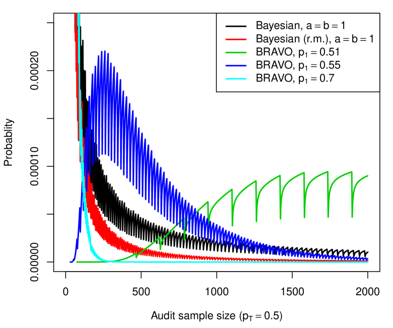
5.1.1 Sample size distributions.

Different methods have different distributions of sample sizes; Figure 1 shows these for a few methods when $p_{T}=0.5$. Some methods tend to stop early; others take many more samples. Requiring a minimum sample size might improve performance of some of the methods; see Section 5.3.

Figure 1: Sample size distributions. Audits of elections with $N=20,000$ ballots, maximum sample size $m=2,000$, and true vote share a tie ($p_{T}=0.5$). Each method is calibrated to have maximum risk 5%. The depicted probabilities all sum to 0.05; the remaining 0.95 probability in each case is on the event that the audit reaches the full sample size ($n=m$) and progresses to a full manual tabulation. ‘Bayesian (r.m.)’ refers to the Bayesian audit with a risk-maximizing prior. The sawtooth pattern is due to the discreteness of the statistics.

5.1.2 Mean sample sizes.

We focus on average sample sizes as a measure of audit efficiency. Table 2 shows the results of experiments with $N=20,000$ and $m=2,000$. We discuss other experiments and performance measures below.

Table 2: Results from benchmarking experiments. Audits of elections with $N=20,000$ ballots and a maximum sample size $m=2,000$. The numeric column headings refer to the value of $p_{T}$; the corresponding margin of victory (mov) is also reported. Each row refers to a specific auditing method. For calibrated methods, we report the threshold obtained. For easier comparison, we present these on the nominal risk scale for BRAVO, MaxBRAVO and ClipAudit (e.g. $\alpha=1/h$ for BRAVO), and on the upset probability scale for the Bayesian methods ($\upsilon=1/(h+1)$). For the experiments without calibration, we report the maximum risk of each method when set to a ‘nominal’ risk limit of 5%. We only report uncalibrated results for methods that are automatically risk-limiting, as well as ClipAudit using its ‘best fit’ formula to set the threshold. ‘Bayesian (r.m.)’ refers to the Bayesian audit with a risk-maximizing prior. The numbers in bold are those that are (nearly) best for the given experiment and choice of $p_{T}$. The section labelled ‘$n\geqslant 300$’ refers to experiments that required the audit to draw at least 300 ballots.

		Power (%)				Mean sample size
	$p_{T}$ (%) $\rightarrow$	52	55	60		52	55	60	64	70
Method	mov (%) $\rightarrow$	4	10	20		4	10	12	28	40
Calibrated	$\alpha$ or $\upsilon$ (%)
Bayesian, $a=b=1$	0.2	35	99	100		1623	637	172	90	46
Bayesian, $a=b=100$	1.2	48	100	100		1551	616	232	150	97
Bayesian, $a=b=500$	3.6	53	100	100		1582	709	318	219	149
Bayesian (r.m.), $a=b=1$	6.1	19	94	100		1742	813	185	89	41
BRAVO, $p_{1}=0.7$	5.8	9	21	84		1828	1592	530	95	37
BRAVO, $p_{1}=0.55$	5.3	37	99	100		1549	562	196	129	85
BRAVO, $p_{1}=0.51$	22.7	55	100	100		1617	791	384	272	190
MaxBRAVO	1.6	30	98	100		1660	680	177	91	45
ClipAudit	4.7	33	98	100		1630	639	169	89	45
Calibrated, $n\geqslant 300$	$\alpha$ or $\upsilon$ (%)
Bayesian, $a=b=1$	0.6	45	99	100		1547	601	311	300	300
Bayesian (r.m.), $a=b=1$	34.4	39	99	100		1554	587	307	300	300
BRAVO, $p_{1}=0.7$	100.0	0	6	83		1994	1900	708	309	300
BRAVO, $p_{1}=0.55$	6.0	38	99	100		1545	583	309	300	300
BRAVO, $p_{1}=0.51$	22.7	55	100	100		1617	791	392	313	300
MaxBRAVO	5.0	44	99	100		1546	595	310	300	300
ClipAudit	11.4	44	99	100		1545	595	310	300	300
Uncalibrated	Risk (%)
Bayesian (r.m.), $a=b=1$	3.7	17	93	100		1785	864	198	95	44
BRAVO, $p_{1}=0.7$	4.3	8	20	83		1846	1621	552	99	38
BRAVO, $p_{1}=0.55$	4.7	37	98	100		1561	572	200	131	86
BRAVO, $p_{1}=0.51$	0.029	6	89	100		1985	1505	760	542	377
ClipAudit	5.1	34	98	100		1618	628	167	88	45

No method was uniformly best. Given the equivalence of BRAVO and Bayesian audits, the comparisons amount to examining dependence on the prior.

In general, methods that place more weight on close elections, such as BRAVO with $p_{1}=0.55$ or a Bayesian audit with a moderately constrained prior ($a=b=100$) were optimal when $p_{T}$ was closer to 0.5. Methods with substantial prior weight on wider margins, such as BRAVO with $p_{1}=0.7$ and Bayesian audits with the risk-maximizing prior, perform poorly for close elections.

Consistent with theory, BRAVO was optimal when the assumptions matched the truth ($p_{1}=p_{T}$). However, our experiments violate the theoretical assumptions because we imposed a maximum sample size, $m$. (Indeed, when $p_{1}=p_{T}=0.51$, BRAVO is no longer optimal in our experiments.)

Two methods were consistently poor: BRAVO with $p_{1}=0.51$ and a Bayesian audit with $a=b=500$. Both place substantial weight on a very close election.

MaxBRAVO and ClipAudit, the two methods without a direct match to Bayesian audits, performed similarly to a Bayesian audit with a uniform prior ($a=b=1$). All three are ‘broadly’ tuned: they perform reasonably well in most scenarios, even when they are not the best.

5.1.3 Effect of calibration on the uncalibrated methods.

For most of the automatically calibrated methods, calibration had only a small effect on performance. BRAVO with $p_{1}=0.51$ is an exception: it was very conservative because it normally requires more than $m$ samples.

5.1.4 Other election sizes and performance measures.

The broad conclusions are the same for a range of values of $m$ and $N$, and when performance is measured by quantiles of sample size or probability of stopping without a full hand count rather than by average sample size.

5.1.5 Sampling with vs without replacement.

There are two ways to change our experiments to explore sampling with replacement: (i) construct versions of the statistics specifically for sampling with replacement; (ii) leave the methods alone but sample with replacement. We explored both options, separately and combined; differences were minor when $m\ll N$.

5.2 Choosing between methods

Consider the following two methods, which were the most efficient for different election margins: (i) BRAVO with $p_{1}=0.55$; (ii) ClipAudit. For $p_{T}=0.52$, the mean sample sizes are 1,549 vs 1,630 (BRAVO saved 81 draws on average). For $p_{T}=0.7$, the equivalent numbers are 85 vs 45 (ClipAudit saved 40 draws on average).

Picking a method requires trade-offs involving resources, workload predictability, and jurisdictional idiosyncrasies in ballot handling and storage—as well as the unknown true margin. Differences in expected sample size across ballot-polling methods might be immaterial in practice compared to other desiderata.

5.3 Exploring changes to the methods

5.3.1 Increasing the sampling increment (‘round size’).

Increasing the number of ballots sampled in each ‘round’ increases the chance that the audit will stop without a full hand count but increases mean sample size. This is as expected; the limiting version is a single fixed sample of size $n=m$, which has the highest power but loses the efficiency that early stopping can provide.

Increasing the sampling increment had the most impact on methods that tend to stop early, such as Bayesian audits with $a=b=1$, and less on methods that do not, such as BRAVO with $p_{1}=0.51$. Increasing the increment also decreases the differences among the methods. This makes sense because when the sample size is $m$, the methods are identical (since all are calibrated to attain the risk limit).

Considering the trade-off discussed in the previous section, since increasing the sampling increment improves power but increases mean sample size, it reduces effort when the election is close, but increases it when the margin is wide.

5.3.2 Increasing the maximum sample size ($m$).

Increasing $m$ has the same effect as increasing the sampling increment: higher power at the expense of more work on average. This effect is stronger for closer elections, since sampling will likely stop earlier when the margin is wide.

5.3.3 Requiring/encouraging more samples.

The Bayesian audit with $a=b=1$ tends to stop too early, so we tried two potential improvements, shown in Table 2.

The first was to impose a minimum sample size, in this case $n\geqslant 300$. This is very costly if the margin is wide, since we would not normally require this many samples. However, it boosts the power of this method and reduces its expected sample size for close contests.

A gentler way to achieve the same aim is to make the prior more informative, by increasing $a$ and $b$. When $a=b=100$, we obtain largely the same benefit for close elections with a much milder penalty when the margin is wide. The overall performance profile becomes closer to BRAVO with $p_{1}=0.55$.

6 Discussion

We compared several ballot-polling methods both analytically and numerically, to elucidate the relationships among the methods. We focused on two-candidate contests, which are building blocks for auditing more complex elections. We explored modifications and extensions to existing procedures. Our benchmarking experiments calibrated the methods to attain the same maximum risk.

Many ‘non-Bayesian’ auditing methods are special cases of a Bayesian procedure for a suitable prior, and Bayesian methods can be calibrated to be risk-limiting (at least, in the two-candidate, all-valid-vote context investigated here). Differences among such methods amount to technical details, such as choices of tuning parameters, rather than something more fundamental. Of course, upset probability is fundamentally different from risk.

No method is uniformly best, and most can be ‘tuned’ to improve performance for elections with either closer or wider margins—but not both simultaneously. If the tuning is not extreme, performance will be reasonably good for a wide range of true margins. In summary:

1. If the true margin is known approximately, BRAVO is best.

2. Absent reliable information on the margin, ClipAudit and Bayesian audits with a uniform prior (calibrated to attain the risk limit) are efficient.

3. Extreme settings, such as $p_{1}\approx 0.5$ or an overly informative prior may result in poor performance even when the margin is small. More moderate settings give reasonable or superior performance if the maximum sample size is small compared to the number of ballots cast.

Choosing a method often involves a trade-off in performance between narrow and wide margins.

There is more to auditing than the choice of statistical inference method. Differences in performance across many ‘reasonable’ methods are small compared to other factors, such as how ballots are organized and stored.

Future work: While we tried to be comprehensive in examining ballot-polling methods for two-candidate contests with no invalid votes, there are many ways to extend the analysis to cover more realistic scenarios. Some ideas include: (i) more than two candidates and non-plurality social choice functions; (ii) invalid votes; (iii) larger elections; (iv) stratified samples; (v) batch-level audits; (vi) multi-page ballots.

Appendix 0.A Risk-limiting Bayesian audits with arbitrary priors

All of the results in this appendix are for ballot-polling audits of two-candidate contests with no invalid votes, the same as for the main text of this paper. For brevity, we often omit stating this assumption in the mathematical statements below.

For such contests, Vora [11] provided a construction of a risk-limiting Bayesian audit, by taking a Bayesian audit with an arbitrary prior and constructing a new prior from it that has the property that a threshold on the upset probability is also a risk limit.

We extend that result to show that any prior has a bounded maximum risk and can therefore be used to conduct a risk-limiting audit. Such a usage would involve calculating a threshold on the upset probability that gives a particular specified bound on the risk. Our derivation also applies to a more general class of Bayesian audits than considered by Vora [11].

First, we need to define some more general procedures and further notation.

0.A.1 General SPRT and Bayesian audits

The SPRT-based and Bayesian audits presented in the main text only terminate sampling in order to certify the election. More generally, we can specify a threshold of evidence for terminating the sampling and proceeding immediately to a full manual tabulation (similar to reaching the sample size limit, $m$, but the threshold could be reached much earlier).

The SPRT-based audit, as per Wald’s original definition, is as follows:

$$\begin{cases}\text{if }S_{n}>\frac{1-\beta}{\alpha},&\text{terminate and certify,}\\ \text{if }S_{n}<\frac{\beta}{1-\alpha},&\text{proceed to full tabulation,}\\ \text{otherwise,}&\text{continue sampling.}\\ \end{cases}$$

The statistic $S_{n}$ is the likelihood ratio, the same as our earlier definition from Section 3.2. The only new component here is $\beta$. When $\beta=0$, we recover the earlier definition, noting that the second inequality here will never be satisfied because $S_{n}$ cannot be negative. Like the earlier definition, this version of the SPRT has a risk limit of $\alpha$.

Analogously, we define a more general Bayesian audit as follows:

$$\begin{cases}\text{if }S_{n}>\frac{1-\upsilon}{\upsilon},&\text{terminate and certify,}\\ \text{if }S_{n}<\frac{1-\phi}{\phi},&\text{proceed to full tabulation,}\\ \text{otherwise,}&\text{continue sampling.}\\ \end{cases}$$

The statistic $S_{n}$ is the Bayes factor, the same as our earlier definition from Section 3.1. If the prior gives equal weight to the two hypotheses, $\Pr(H_{0})=\Pr(H_{1})$, then the inequalities above are equivalent to more straightforward ones in terms of the upset probability, as follows:

$$\begin{cases}\text{if }\Pr(H_{0}\mid Y_{n})<\upsilon,&\text{terminate and certify,}\\ \text{if }\Pr(H_{0}\mid Y_{n})>\phi,&\text{proceed to full tabulation,}\\ \text{otherwise,}&\text{continue sampling.}\\ \end{cases}$$

Setting $\phi=1$ recovers our earlier definition of the Bayesian audit.

0.A.2 Correspondence between the SPRT and Bayesian audits

In Section 3.2, we noted that the SPRT is equivalent to a Bayesian audit with a particular choice of prior (equal point masses on $p_{0}$ and $p_{1}$) and a specific choice of threshold. We can extend this correspondence to the more general definitions above. We keep the choice of prior the same (equal point masses)—this makes $S_{n}$ equivalent under both audit methods—and equate the two sets of thresholds,

$$\frac{1-\beta}{\alpha}=\frac{1-\upsilon}{\upsilon}\quad\text{and}\quad\frac{\beta}{1-\alpha}=\frac{1-\phi}{\phi}.$$

We can solve these for either $\alpha$ and $\beta$, or $\upsilon$ and $\phi$, which respectively gives:

$$\alpha =\frac{\upsilon(2\phi-1)}{\phi-\upsilon} \upsilon =\frac{\alpha}{1-\beta+\alpha}$$

$$\beta =\frac{(1-\phi)(1-2\upsilon)}{\phi-\upsilon} \phi =\frac{1-\alpha}{1-\beta+\alpha}.$$

In other words, the SPRT is equivalent to a Bayesian audit with a prior having equal point masses on $p_{0}$ and $p_{1}$, and the thresholds $\upsilon$ and $\phi$ set to the values given above (in terms of the desired $\alpha$ and $\beta$).

As a corollary, a Bayesian audit with such a prior will have a risk limit given by $\upsilon(2\phi-1)/(\phi-\upsilon)$.

0.A.2.1 Special cases.

The results in the main text were for the special case where $\beta=0$ and $\phi=1$. Under this case, the above correspondence with the SPRT simplifies to $\alpha=\upsilon/(1-\upsilon)$ and $\upsilon=\alpha/(1+\alpha)$.

Vora [11] considered a more restricted version of the Bayesian audit where $\phi=1-\upsilon$ (symmetric thresholds on the upset probability). This is a special case of the general definition given here. Under this special case, the above correspondence with the SPRT simplifies to $\alpha=\beta=\upsilon$ (the risk limit is the same the the threshold on the upset probability).

The relative sizes of the risk limit ($\alpha$) and the upset probability threshold ($\upsilon$) are sometimes of interest. It is instructive to look at the correspondence with the SPRT and consider different cases. In the special case in the main text, we have $\alpha=\upsilon/(1-\upsilon)>\upsilon$; the risk limit is larger than the threshold. For Vora’s special case, the two values coincide. We can also construct audits where the risk limit is smaller than the threshold by setting $\phi<1-\upsilon$; such audits are more likely to terminate early and proceed to a full tabulation, hence reducing the risk.

0.A.2.2 The risk-maximizing prior.

Vora [11] defined a ‘risk-maximising prior’ in order to construct a Bayesian audit for which the threshold on the upset probability was also a risk limit. From the more general analysis above, we see that this construction relies on symmetric thresholds ($\phi=1-\upsilon$) and will not work in general. For example, in the special case considered in the main text here, to obtain a risk limit of $\alpha$ we need to set a stricter threshold on the upset probability: $\upsilon=\alpha/(1+\alpha)<\alpha$. In terms of the Bayes factor, this translates to: $S_{n}>1/\alpha$.

0.A.3 Further definitions and notation

An audit will result in a sequence of $n$ sampled ballots. The sequence ends either once the audit termination condition is met resulting in the certification of the election, or otherwise once it has progressed to a full manual tabulation of the votes (e.g. upon reaching $n=m$ without certification). Let the $\Lambda$ be the set of all sequences that lead to certification, and $\bar{\Lambda}$ the set of all those that do not.

When the reported winner is not the true winner, the sequences in $\Lambda$ will result in miscertification while those in $\bar{\Lambda}$ will lead to discovering the true winner. The risk of the audit will be the probability of obtaining a sequence from $\Lambda$ (rather than $\bar{\Lambda}$). In other words,

$$\Pr(\text{certify}\parallel T,N)=\sum_{s\in\Lambda}\Pr(s\parallel T,N),$$ (1)

where $s=(X_{1},X_{2},\dots,X_{n})$ here represents an arbitrary sequence that leads to certification, and as before $T$ is the true total number of votes for the winner and $N$ the total number of cast ballots. Note that $n$ is not fixed; different sequences can terminate at different values of $n$. The summand is the probability of observing a specific sequence. If sampling with replacement, this will be a product of Bernoulli probabilities,

$$\Pr(s\parallel T,N)=\Pr(s\parallel p_{T})=p_{T}^{Y_{n}}(1-p_{T})^{n-Y_{n}}.$$ (2)

Note that this is the same a binomial probability but without the binomial coefficient, $\binom{n}{Y_{n}}$. It represent the probability of a given ordered sequence of ballots. If sampling without replacement, the probability of the sequence will be an ordered version of a hypergeometric probability,

$$\Pr(s\parallel T,N)=\frac{1}{\binom{n}{Y_{n}}}\frac{\binom{T}{Y_{n}}\binom{N-T}{n-Y_{n}}}{\binom{N}{n}}=\frac{T^{(Y_{n})}(N-T)^{(n-Y_{n})}}{N^{(n)}},$$ (3)

using the notation $n^{(m)}=n(n-1)\cdots(n-m+1)=n!/(n-m)!$.

Before we state the main results of this appendix, we define a property of the auditing methods that we need for later proofs.

Definition 1

An auditing method is called sample-coherent if for every sequence that results in certification ($s\in\Lambda$), the sampled final tally will be in favour of the reported winner, i.e. $Y_{n}/n>0.5$.

This property would be expected of any sensible auditing method, but is not mathematically guaranteed. Indeed, it is possible to define stopping rules for an audit such that this property does not hold. Here, we only consider sample-coherent auditing methods.

0.A.4 Bayesian audits are risk-limiting

Lemma 1

The maximum risk of a sample-coherent ballot-polling audit of a plurality contest with two candidates and no invalid votes is given by the (mis)certification probability when the true tally gives equal votes for each candidate ($T=\frac{N}{2}$, $p_{T}=\frac{1}{2}$), or the closest possible such non-winning tally in the case where we have odd number of cast ballots ($T=\frac{N-1}{2}$).

Proof

We prove this lemma by showing the summand in (1) is monotonically increasing in $T$ when $H_{0}$ is true. This is the same technique used to prove Theorem 2 in Vora [11], for the case of $N$ odd and sampling without replacement. Here we extend the argument to also cover $N$ even and sampling with replacement.

For sampling with replacement, the summand is given by (2). As a function of $p_{T}$ over the unit interval, this is strictly increasing until it reaches a maximum at $p_{T}=Y_{n}/n$ and strictly decreasing thereafter. This is easily shown via calculus (note also that (2) is a binomial likelihood with $Y_{n}/n$ as the corresponding maximum likelihood estimate). By 1, this maximum occurs at a value $p_{T}>0.5$. Therefore, when $H_{0}$ is true ($p_{T}\leqslant 0.5$), the summand is monotonically increasing in $p_{T}$, and therefore also in $T$.

For sampling without replacement, the summand is given by (3). Consider this as a function of $T$. We will increment this by 1 (replacing $T$ with $T+1$), take the ratio with the original version, and show this ratio is positive. Let the ratio be $G$. We have

$$G=\frac{\Pr(s\parallel T+1,N)}{\Pr(s\parallel T,N)}=\frac{T+1}{T-Y_{n}+1}\times\frac{(N-T)-(n-Y_{n})}{N-T}.$$

We assume that $H_{0}$ is still true when $T$ is incremented, that is we have $(T+1)/N\leqslant 0.5$. Also, by 1 we have $0.5<Y_{n}/n$. Therefore,

$$\frac{T+1}{N}<\frac{Y_{n}}{n}.$$

This inequality still holds if we convert both of these probabilities into odds,

$$\frac{(T+1)/N}{(N-T-1)/N} <\frac{Y_{n}/n}{(n-Y_{n})/n}$$

$$\frac{T+1}{N-T-1} <\frac{Y_{n}}{n-Y_{n}}.$$

We also trivially have

$$\frac{T+1}{N-T}<\frac{T+1}{N-T-1}$$

as long as $N-T>1$, i.e. as long as one vote has been cast in favour of the losing candidate. This will be true for all practical scenarios of interest since $N$ will be large (certainly, much larger than 2), and under $H_{0}$ we must have $T$ be at most $N/2$.

Combining the previous two inequalities gives,

$$\frac{T+1}{N-T} <\frac{Y_{n}}{n-Y_{n}}$$

$$\frac{n-Y_{n}}{N-T} <\frac{Y_{n}}{T+1}$$

$$1-\frac{Y_{n}}{T+1} <1-\frac{n-Y_{n}}{N-T}$$

$$\frac{T+1-Y_{n}}{T+1} <\frac{(N-T)-(n-Y_{n})}{N-T}$$

$$1 <\frac{T+1}{T+1-Y_{n}}\times\frac{(N-T)-(n-Y_{n})}{N-T}=G.$$

In other words, the ratio is positive. Therefore, the summand given by (3) is monotonically increasing in $T$ as long as $H_{0}$ is true. ∎

Lemma 2

The risk of a Bayesian audit is a monotone increasing function of $\upsilon$, the threshold on the upset probability. In other words, relaxing the threshold leads to greater risk.

Proof

If $\upsilon$ is increased (i.e. less stringent evidence threshold), then:

• Any sequence in $\Lambda$ remains in $\Lambda$, since if it passed the earlier, stricter threshold then it will also pass the newer, looser one. The only change will be that the audit possibly terminates earlier (i.e. the sample size at which the audit stops is reduced).

• Some sequences in $\bar{\Lambda}$ move to $\Lambda$, because they now meet the newer, relaxed threshold.

Therefore, overall there will be a shift of probability from $\bar{\Lambda}$ to $\Lambda$. Therefore the risk has increased. Note that this is true for any value of $T$, including for the value that maximises the risk. ∎

Note that 2 also holds for any audit procedure with a stopping rule of the form, “stop if $f(\text{sample data})\geqslant\upsilon$”. A Bayesian audit is just one such procedure.

Corollary 1

For any prior, Bayesian ballot-polling audits of a two-candidate, no invalid vote plurality contest can be calibrated to be risk-limiting, in the sense that for any risk limit $\alpha\in(0,1)$, there exists $\upsilon\in(0,1)$ such that terminating the audit when the upset probability is not greater than $\upsilon$ limits the risk of the procedure to $\alpha$. (Typically, this requires $\upsilon<\alpha$.)

Proof

1 shows that any Bayesian audit has a bounded maximum risk. The monotonic relationship from 2 implies that we can reduce this risk by imposing a stricter threshold on the upset probability. In particular, we can reduce it until the maximum risk is less than any pre-specified limit. Thus, we can use any Bayesian audit in a risk-limiting fashion. ∎

To implement this in practice we need to be able calculate the maximum risk for any given threshold and optimise the threshold value until this risk is smaller than the specified limit. This is straightforward for the two-candidate case via either simulation or exact calculation, since we know the value of $T$ that gives rise to the maximum risk. Such a calculation would need to be done separately for any given choice of sampling scheme and prior.

Appendix 0.B KMart as a Bayesian audit

This appendix shows a proof that for sampling with replacement, KMart is equivalent to a Bayesian audit with a risk-maximising prior for the reported winner’s true vote tally, uniform on $(\frac{1}{2},1]$. It also introduces a more general version of the test statistic that corresponds to an arbitrary risk-maximising prior. Both results are shown for a simple two-candidate contest.

0.B.1 KMart is equivalent to a Bayesian audit

As in Section 3.4, we let $t=\operatorname{\mathbb{E}}(X_{1}\parallel H_{0})$, the true proportion of votes for the reported winner under the null hypothesis. Since we assume sampling without replacement, $\{X_{i}\}$ is a sequence of Bernoulli trials with success probability $t$ if the null is true. As explained previously, we set $t=0.5$ since that is the incorrect outcome for which the risk of the method is largest.

In practice we will always have a finite number of total votes, and thus a realistic model would have the support of $t$ be a discrete set (i.e. values of the form $k/N$, where $k$ is the total number of votes in favour of the reported winner). However, for mathematical convenience here we will allow the support of $t$ to be the unit interval, which is continuous.

To distinguish the test statistics ($S_{n}$) from KMart and Bayesian audits, we will refer to the KMart statistic by $A_{n}$ and the Bayesian statistic by $B_{n}$.

0.B.1.1 KMart audits.

For sampling with replacement, the KMart statistic is:

$$A_{n}=\int_{0}^{1}\prod_{i=1}^{n}\left(\gamma\left[\frac{X_{i}}{t}-1\right]+1\right)d\gamma.$$

Since we are working with $t=\frac{1}{2}$, we can rewrite this expression,

$$A_{n}=2^{n}\int_{0}^{1}\prod_{i=1}^{n}\left(\gamma\left[X_{i}-\frac{1}{2}\right]+\frac{1}{2}\right)d\gamma.$$

For a specified risk limit, $\alpha$, the audit proceeds until $A_{n}>1/\alpha$, at which point the election is certified ($H_{0}$ is rejected), or is otherwise terminated in favour of doing a full manual tabulation.

0.B.1.2 Bayesian audits.

The Bayesian statistic is the BF:

$$B_{n}=\frac{\Pr(X_{1},\dots,X_{n}\mid H_{1})}{\Pr(X_{1},\dots,X_{n}\mid H_{0})}.$$

For sampling with replacement, the likelihood is the product of Bernoulli mass functions and can be written completely in terms of $Y_{n}$, the total number of sampled votes in favour of the winner,

$$\Pr(X_{1},\dots,X_{n}\mid p)=p^{Y_{n}}(1-p)^{n-Y_{n}}.$$

We limit our discussion to risk-maximising prior distributions. Reminder: these place a probability mass of $\frac{1}{2}$ on the value of $p=\frac{1}{2}$, and the remaining probability is over the set $p\in(\frac{1}{2},1]$.

The denominator of the BF is simple: the likelihood of the sample at the (point) null value,

$$\Pr(X_{1},\dots,X_{n}\mid H_{0})=\Pr\left(X_{1},\dots,X_{n}\mid p=\tfrac{1}{2}\right)=\left(\tfrac{1}{2}\right)^{Y_{n}}\left(\tfrac{1}{2}\right)^{n-Y_{n}}=1/2^{n}.$$

The numerator requires integrating over the prior under $H_{1}$,

$$\Pr(X_{1},\dots,X_{n}\mid H_{1})=\int_{\frac{1}{2}}^{1}p^{Y_{n}}\left(1-p\right)^{n-Y_{n}}f(p)\,dp.$$

Putting these together gives,

$$B_{n}=2^{n}\int_{\frac{1}{2}}^{1}p^{Y_{n}}\left(1-p\right)^{n-Y_{n}}f(p)\,dp.$$

Similar to KMart, a Bayesian audit proceeds until $B_{n}>1/\alpha$.

0.B.1.3 Equivalence.

Both $A_{n}$ and $B_{n}$ are expressed as integrals but with the $X_{i}$ in different ‘places’ in the integrand. The key to showing they are equivalent is to notice that the $X_{i}$ are binary variables, which allows us to set up an identity that relates the two ways of writing the integral. Specifically, we have the following identity,

$$\gamma\left(X_{i}-\frac{1}{2}\right)+\frac{1}{2}=\left(\frac{1+\gamma}{2}\right)^{X_{i}}\left(\frac{1-\gamma}{2}\right)^{1-X_{i}}.$$

This allows us to rewrite $A_{n}$,

$$A_{n}=2^{n}\int_{0}^{1}\left(\frac{1+\gamma}{2}\right)^{Y_{n}}\left(\frac{1-\gamma}{2}\right)^{n-Y_{n}}d\gamma=\int_{0}^{1}\left(1+\gamma\right)^{Y_{n}}\left(1-\gamma\right)^{n-Y_{n}}d\gamma.$$

Next, let $\gamma=2p-1$ and change the variable of integration,

$$A_{n}=\int_{\frac{1}{2}}^{1}(2p)^{Y_{n}}(2-2p)^{n-Y_{n}}2\,dp=2^{n}\int_{\frac{1}{2}}^{1}p^{Y_{n}}\left(1-p\right)^{n-Y_{n}}2\,dp.$$

Finally, note that this is identical to $B_{n}$ if we set the prior to be uniform over $H_{1}$, i.e. $f(p)=2$.

In other words, a KMart audit is equivalent to a Bayesian audit that uses a risk-maximising prior that is uniform on $(\frac{1}{2},1]$.

0.B.2 Extending KMart to arbitrary priors

From the above result, we can see that $\gamma$ plays a similar role to $p$. The somewhat arbitrary integral over $\gamma$ used to define $A_{n}$ can be generalised by specifying a weighting function $g(\gamma)$,

$$A_{n}=\int_{0}^{1}\prod_{i=1}^{n}\left(\gamma\left[\frac{X_{i}}{t}-1\right]+1\right)g(\gamma)\,d\gamma.$$

Applying the same transformations as above gives

$$A_{n}=2^{n}\int_{\frac{1}{2}}^{1}p^{Y_{n}}\left(1-p\right)^{n-Y_{n}}2\times g(2p-1)\,dp.$$

In other words, this generalised version of KMart is equivalent to a Bayesian audit with the following risk-maximising prior:

$$f(p)=2\times g(2p-1).$$

The original KMart is the special case where $g(\cdot)=1$.

0.B.3 Efficient computation by exploiting the equivalence

We can use the above equivalence to develop fast ways to compute the KMart statistic (when sampling with replacement), by relating it to standard Bayesian calculations using conjugate priors.

First, we show that if we take a conjugate prior distribution, truncate it, and add some point masses, the resulting distribution is still conjugate. Then we use this result to write a formula for the posterior distribution for the same case as above (simple two-candidate election, sampling with replacement).

0.B.3.1 Truncation and point masses preserve conjugacy.

(The proofs shown here are not too hard to derive and may well be described elsewhere.)

Suppose we have a single parameter, $\theta$, some data, $D$, a likelihood function, $L(\theta\mid D)$, and a conjugate prior distribution, $f(\theta)$. That means we have,

$$f(\theta\mid D)\propto L(\theta\mid D)f(\theta).$$

Let the normalising constant be,

$$k=\int L(\theta\mid D)f(\theta)d\theta.$$

This allows us to express the posterior as,

$$f(\theta\mid D)=\frac{1}{k}L(\theta\mid D)f(\theta),$$

The sections that follow each start with these definitions and transform the prior in various ways.

Truncation.

Truncate the prior to a subset $S$ (i.e. we only allow $\theta\in S$). Write this truncated prior as,

$$f^{*}(\theta)=f(\theta)\frac{I_{S}(\theta)}{z_{S}},$$

where $I_{S}(\theta)$ is the indicator function that takes value 1 when $\theta\in S$, and $z_{S}=\int f(\theta)I_{S}(\theta)d\theta=\int_{S}f(\theta)d\theta$ is the normalising constant due to truncation.

If we use this prior, we get the posterior

$$f^{*}(\theta\mid D)=\frac{1}{k^{*}}L(\theta\mid D)f^{*}(\theta),$$

where,

$$k^{*}=\int L(\theta\mid D)f^{*}(\theta)d\theta.$$

Expanding this out gives,

$$f^{*}(\theta\mid D)=\frac{1}{k^{*}z_{S}}L(\theta\mid D)f(\theta)I_{S}(\theta)=\frac{k}{k^{*}z_{S}}f(\theta\mid D)I_{S}(\theta).$$

This is the original posterior truncated to $S$. Thus, the truncation results in staying within the same family of (truncated) probability distributions, which means this family is conjugate.

Adding a point mass.

Define a ‘spiked’ prior where we add a point mass at $\theta_{0}$,

$$f^{*}(\theta)=u\,\delta_{\theta_{0}}(\theta)+vf(\theta),$$

where $u+v=1$. In other words, a mixture distribution with mixture weights $u$ and $v$. The normalising constant is,

$$k^{*}=\int L(\theta\mid D)f^{*}(\theta)d\theta=uL(\theta_{0}\mid D)+vk.$$

We can write the posterior as,

$$f^{*}(\theta\mid D)=\frac{1}{k^{*}}L(\theta\mid D)f^{*}(\theta)=\frac{u\,L(\theta_{0}\mid D)}{k^{*}}\delta_{\theta_{0}}(\theta)+\frac{vk}{k^{*}}f(\theta\mid D).$$

This is a ‘spiked’ version of the original posterior. You can see this more clearly by defining,

$$u^{*}=\frac{u\,L(\theta_{0}\mid D)}{k^{*}},\quad v^{*}=\frac{vk}{k^{*}},$$

where $u^{*}+v^{*}=1$. Thus, ‘spiking’ a distribution results in a conjugate family. Note that the mixture weights get updated as we go from the prior to the posterior.

Truncating and adding point masses.

We can combine both of the previous operations and we will still retain conjugacy. In fact, due to the generality of the proof, we can apply each one an arbitrary number of times, e.g. to add many point masses.

0.B.3.2 Application to KMart.

When sampling with replacement, the conjugate prior for $p$ is a beta distribution.

We showed earlier that KMart was equivalent to using a risk-maximising prior. Starting with any beta distribution, we can form the corresponding risk-maximising prior by truncating to $p\in(\frac{1}{2},1]$ and adding a probability mass of $\frac{1}{2}$ at $p=\frac{1}{2}$. Based on the argument presented above, this prior is conjugate. Moreover, we can express the posterior in closed form.

Let the original prior be $p\sim\text{Beta}(a,b)$. The risk-maximising prior retains the functional form of this prior for $p>\frac{1}{2}$ and also has a mass of $\frac{1}{2}$ at $p=\frac{1}{2}$.

After we observe a sample of size $n$ from the audit, we have a posterior with an updated probability mass at $p=\frac{1}{2}$. This mass will be the upset probability. We can derive an expression for it using equations similar to above (it will correspond to $u^{*}$ using the notation from above).

Let $f(p)$ be the pdf of the original beta prior, $F(p)$ be its cdf, $S=(\frac{1}{2},1]$ the truncation region, $F^{\prime}(p)$ the cdf of the beta-distributed portion of the posterior (i.e. the posterior distribution if we use the original beta prior), and $B(\cdot,\cdot)$ be the beta function. We have,

$$k^{*}=\frac{1}{2}\left(\frac{1}{2}\right)^{n}+\frac{1}{2}\frac{k^{\prime}}{z_{S}},$$

where

$$z_{S}=\int_{\frac{1}{2}}^{1}f(p)dp=1-F\left(\frac{1}{2}\right)$$

and

$$k^{\prime}=\int_{\frac{1}{2}}^{1}L(p\mid D)f(p)dp=\frac{B(Y_{n}+a,n-Y_{n}+b)}{B(a,b)}\left(1-F^{\prime}\left(\frac{1}{2}\right)\right).$$

Putting these together gives,

$$k^{*}=\frac{1}{2^{n+1}}+\frac{1}{2}\times\frac{B(Y_{n}+a,n-Y_{n}+b)}{B(a,b)}\times\frac{1-F^{\prime}\left(\frac{1}{2}\right)}{1-F\left(\frac{1}{2}\right)}.$$

The upset probability is,

$$u^{*}=\frac{\frac{1}{2^{n+1}}}{k^{*}}.$$

These quantities will be straightforward to calculate as long we have efficient ways to calculate:

1. The beta function.

2. The cdf of a beta distribution.

Both have fast implementations in R.

References

- [1] Blom, M., Stuckey, P.J., Teague, V.J.: Ballot-polling risk limiting audits for IRV elections. In: Electronic Voting. pp. 17–34. Springer, Cham (2018)
- [2] Kulldorff, M., Davis, R.L., Kolczak, M., Lewis, E., Lieu, T., Platt, R.: A maximized sequential probability ratio test for drug and vaccine safety surveillance. Sequential Analysis 30(1), 58–78 (2011). https://doi.org/10.1080/07474946.2011.539924
- [3] Lindeman, M., Stark, P.B., Yates, V.S.: BRAVO: Ballot-polling risk-limiting audits to verify outcomes. In: 2012 Electronic Voting Technology Workshop/Workshop on Trustworthy Elections (EVT/WOTE ’12) (2012)
- [4] National Academies of Sciences, Engineering, and Medicine: Securing the Vote: Protecting American Democracy. The National Academies Press, Washington, DC (Sep 2018). https://doi.org/10.17226/25120
- [5] Rivest, R.L.: ClipAudit: A simple risk-limiting post-election audit. arXiv e-prints arXiv:1701.08312 (Jan 2017)
- [6] Rivest, R.L., Shen, E.: A Bayesian method for auditing elections. In: 2012 Electronic Voting Technology/Workshop on Trustworthy Elections (EVT/WOTE ’12) (2012)
- [7] Stark, P.: Conservative statistical post-election audits. Ann. Appl. Stat. 2, 550–581 (2008), http://arxiv.org/abs/0807.4005
- [8] Stark, P.: Sets of half-average nulls generate risk-limiting audits: SHANGRLA. Voting ’20 in press (2020), preprint: http://arxiv.org/abs/1911.10035
- [9] Stark, P.B.: Risk-limiting postelection audits: Conservative -values from common probability inequalities. IEEE Transactions on Information Forensics and Security 4(4), 1005–1014 (Dec 2009). https://doi.org/10.1109/TIFS.2009.2034190
- [10] Stark, P.B., Teague, V.: Verifiable European elections: Risk-limiting audits for D’Hondt and its relatives. USENIX Journal of Election Technology and Systems (JETS) 1(3), 18–39 (Dec 2014), https://www.usenix.org/jets/issues/0301/stark
- [11] Vora, P.L.: Risk-Limiting Bayesian Polling Audits for Two Candidate Elections. arXiv e-prints arXiv:1902.00999 (Feb 2019)
- [12] Wald, A.: Sequential tests of statistical hypotheses. Ann. Math. Statist. 16(2), 117–186 (June 1945). https://doi.org/10.1214/aoms/1177731118