Instance-Aware Graph Convolutional Network for Multi-Label Classification
Abstract.
Graph convolutional neural network (GCN) has effectively boosted the multi-label image recognition task by introducing label dependencies based on statistical label co-occurrence of data. However, in previous methods, label correlation is computed based on statistical information of data and therefore the same for all samples, and this makes graph inference on labels insufficient to handle huge variations among numerous image instances. In this paper, we propose an instance-aware graph convolutional neural network (IA-GCN) framework for multi-label classification. As a whole, two fused branches of sub-networks are involved in the framework: a global branch modeling the whole image and a region-based branch exploring dependencies among regions of interests (ROIs). For label diffusion of instance-awareness in graph convolution, rather than using the statistical label correlation alone, an image-dependent label correlation matrix (LCM), fusing both the statistical LCM and an individual one of each image instance, is constructed for graph inference on labels to inject adaptive information of label-awareness into the learned features of the model. Specifically, the individual LCM of each image is obtained by mining the label dependencies based on the scores of labels about detected ROIs. In this process, considering the contribution differences of ROIs to multi-label classification, variational inference is introduced to learn adaptive scaling factors for those ROIs by considering their complex distribution. Finally, extensive experiments on MS-COCO and VOC datasets show that our proposed approach outperforms existing state-of-the-art methods.
The 1907 Franklin Model D roadster.
1. Introduction
As a fundamental task in computer vision, multi-label image recognition aims to accurately and simultaneously recognize multiple objects present in an image. Compared to single-label image classification, multi-label recognition is more challenging because of usually complex scene, more wide label space, and implicit correlation of objects. In view of the natural co-occurrence of objects in the real-world scene, multi-label image classification is more practical than the single-label one, and has received wide attention (Guillaumin et al., 2009; Boutell et al., 2004; Li et al., 2016a; Ge et al., 2018a) in recent years.
Numerous algorithms have been proposed for multi-label image classification. In early works, deep Convolutional Neural Networks (CNNs) used for single-label recognition (Szegedy et al., 2016; He et al., 2016; Huang et al., 2017; Simonyan and Zisserman, 2015) are leveraged for the multi-label task by treating the multi-label recognition as a set of binary classification tasks. Although boosting the accuracy of multi-label classification, however, this type of methods is still limited due to the ignorance of co-occurrence among objects, which can be reflected in label correlation. To model label dependencies, three lines of works have been proposed in recent literatures including attention mechanism based (Szegedy et al., 2016; Wang et al., 2017), recurrent neural network based (Wang et al., 2016), and graph based algorithms (Li et al., 2016b; Li et al., 2014; Chen et al., 2019). Specifically, in graph based methods, graph convolution is introduced to characterize label correlations by diffusing label dependencies with a label correlation matrix (LCM). With graph inference on labels, graph convolutional neural network (GCN) and its variants (Chen et al., 2019; Wang et al., 2020) have reported state-of-the-art performances in recent literatures.
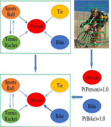
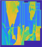
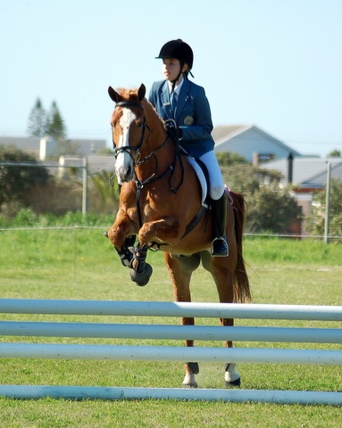
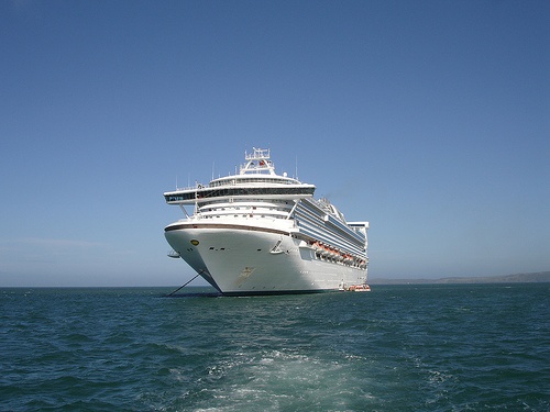
The success of GCN (Kipf and Welling, 2017) indicates the significance of label correlation captured through the LCM for promoting the multi-label classification. In previous GCN (Chen et al., 2019; Wang et al., 2020) based works, the LCM is global and dataset-dependent as it is obtained through the statistic of accessible data. However, in view of the large variation among images, the prior knowledge of label correlation may not well suit for all samples. For instance, the statistical co-occurrence of the bike and person is low, which may mislead the classification for the images of riders. Therefore, individual characteristics of label correlation should also be considered, and used to adaptively modify the prior knowledge. Here, we attempt to construct an adaptive individual LCM for each image instance by utilizing the rough classification scores of ROIs. As shown in Figure 1, as an intuitive understanding, if all ROIs indicate high appearance probabilities of some labels, such as person and bike, then the correlation between person and bike in statistical LCM should be accordingly enhanced for this specific image.
In this paper, we propose an instance-aware graph convolutional neural network (IA-GCN) framework for multi-label classification. The core idea is to adaptively construct one image-dependent label correlation matrix (ID-LCM) for each given image, which better favours the graph inference on labels. For framework construction, considering the previous success of GCN-based methods (Chen et al., 2019; Wang et al., 2020), we build two fused branches of sub-networks in the framework: a global branch modeling the whole image, and an additional region-based branch inferring on ROIs. Moreover, graph inference on labels is conducted to inject label-awareness into the both branches. In this process, different from previous works using statistical LCM (Chen et al., 2019), an image-dependent LCM is constructed by fusing both the statistical LCM and an individual one of each image instance. Specifically, the individual LCM of each image is obtained by mining the label dependencies based on the scores of detected ROIs. Considering the contribution differences of ROIs to multi-label classification, during the generation of the individual LCM, variational inference (Kingma and Welling, 2014) is introduced to learn adaptive scaling factors for those ROIs by considering their complex distribution. As a result, the image-dependent LCM is flexible and benefits the proposed framework in adaptively propagating information on labels for each image instance. Finally, the learned features of both the global and local branches are fused and jointly modeled for the multi-label classification. We test the performance on MS-COCO and VOC datasets, and the results show that our proposed approach outperforms existing state-of-the-art methods.
The main contributions of this paper are as follows:
-
•
We propose a novel IA-GCN framework for the multi-label classification task by jointly modeling the global context of the whole image and local dependencies of ROIs with adaptive information propagation on labels.
-
•
A novel image-dependent LCM is constructed based on both the statistical LCM and an individual one of each image, which endows graph convolution flexibility to handle huge correlation variations among numerous image instances.
-
•
We introduce variational inference to explore label dependencies by considering the distribution of ROI appearances, which results in an adaptive LCM for each image instance.
-
•
We report the state-of-the-art performances on both MS-COCO and VOC datasets, which verifies the effectiveness of our framework.
2. Related work
We first review the related works of multi-label image recognition, and then introduce variational inference and Graph Convolutional Neural Network.
Multi-Label Image Recognition. An initial approach to dealing with multi-label recognition task was to divide it into multiple independent single-label tasks by training a binary classifier for each label. such as the BR method (Tsoumakas and Katakis, 2007) proposed by Tsoumakas. However, the performance of this method is limited by ignoring the correlation among labels. Many researchers proposed various methods for capturing label correlation and have achieved great success. Li et al. (Li et al., 2014) proposed to use probabilistic graph models for formulating the co-occurrence of labels. Gong et al. (Gong et al., 2013) discovered that using a weighted approximated-ranking loss function to train CNN could achieve better performance. Furthermore, Wang et al. (Wang et al., 2016) combined CNN with RNN to learn a joint image-label embedding for characterizing the semantic label dependency and the image-label correlation. In addition, some researchers also applied attention mechanisms to capture label correlation. Wang et al. (Wang et al., 2017) utilized a spatial transformer layer to locate attentional regions and then used long short-term memory (LSTM) to obtain label correlation. Zhu et al. (Zhu et al., 2017) proposed to learn a spatial regularization network in order to explore label relevance.
Variational Inference. There are many problems that are difficult to find their exact solution. Thus, many researchers are committed to finding the approximate solutions of these problems. Variational inference (Kingma and Welling, 2014) is a common method to find the approximate solutions. Agakov (Barber and Agakov, 2003) explored variational bounds on mutual information without considering the objective of the information bottleneck. Mohamed and Rezende (Mohamed and Rezende, 2015) successfully applied variational inference to deep neural networks by exploring the variational boundaries of mutual information based on reinforcement learning. Chalk et al. (Chalk et al., 2016) proposed to achieve nonlinear mapping by the kernel technique and obtained the variational lower bound of the information bottleneck objective. Alexander et al. (Alemi et al., 2016) proposed a Deep VIB model, which applied a neural network to parameterize the information bottleneck model and could obtain an approximate solution of the information bottleneck.
Graph Convolutional Neural Network. The graph is a more effective tool when we explore the correlation of object structure. Li et al. (Li et al., 2014) used the maximum spanning tree algorithm to create a tree-structured label graph. Lee et al. (Lee et al., 2018) utilized knowledge graphs to describe label dependency. Recently, since GCN (Kipf and Welling, 2017) was proposed, it has achieved great success when it was applied to the modeling of non-grid structures. Chen et al. (Chen et al., 2019) built a directed graph of labels and then used GCN to learn an inter-dependent label classifier. Furthermore, Wang et al. (Wang et al., 2020) proposed to superimpose a knowledge prior label graph into a statistical label graph. In this paper, we propose an instance-aware GCN. In detail, firstly, we extract ROIs from each image by Region Proposal Network (RPN) and build an individual LCM for each current image based on the rough labels scores of ROIs. Secondly, we construct an image-dependent LCM fusing both the statistical LCM and an individual LCM of each image instance to adaptively guide information propagation among labels by GCN. Meanwhile, this fused LCM is also used to explore correlation among ROIs by another GCN.
3. Approach
In this part, we first overview the entire IA-GCN architecture, and then introduce four key modules in detail including image-dependent LCM construction, graph convolution on labels, Regions Features Construction and Loss Function.
3.1. Overview
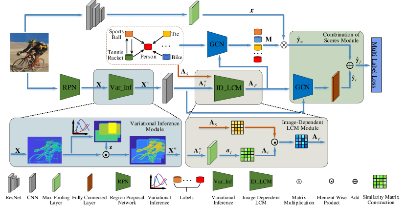
The whole structure of the proposed IA-GCN is illustrated in Figure 2, the purpose of which is to accurately predict the labels of those jointly present objects from given labels. In the learning process, the input image passes through two branches of sub-networks, i.e. a global branch to model the whole image and a region-based branch capturing local dependencies among detected ROIs. For the global branch, considering the success in previous literatures (Chen et al., 2019), we employ ResNet-101 (He et al., 2016) to extract high-level features to describe the context of the whole image. For the region-based branch, we first employ a RPN module (Ren et al., 2015) to generate a fixed number of ROIs and then extract the corresponding features . Considering the contribution differences of those ROIs for multi-label classification, a variational inference module (Kingma and Welling, 2014) is constructed to learn adaptive scaling factors for them. As a result, salient regions for multi-label classification may be highlighted by weighting. Then, the weighted regions endow adaptiveness to the constructed LCMs. In order to inject label-awareness into the two branches above, graph inference is performed on labels with a constructed image-dependent LCM . Specifically, the image-dependent LCM is constructed by fusing a statistical LCM and an individual LCM of each image instance. In detail, the statistical LCM is obtained based on the statistic of accessible training data, and the individual one is constructed based on the rough scores of weighted ROIs. Finally, the two branches are fused to jointly predict the probabilities for those present objects. To optimize the whole framework, multi-label loss is calculated for back-propagation to jointly tune the parameters.
3.2. Image-Dependent LCM Construction
Many exiting works propose to utilize the co-occurrence of labels or the conditional probabilities of labels (Chen et al., 2019) which are both called the statistical information of labels in our paper to construct LCM. However, these methods may be insufficient to handle huge variations among numerous image instances when we just apply global statistical information to guide a single sample. In order to amend these variations, we also need to consider individual labels distribution of each instance. Thus, we integrate the two types labels information for the purpose of achieving their relative balance. In other words, we inject instance information into statistics to realize instance-awareness about labels. We formally present its details as follows.
To achieve label diffusion of instance-awareness and better adaptively guide information propagation among labels, we construct an image-dependent LCM , which is generated by dot product between and .
| (1) |
For the , we construct it by the method of ML-GCN (Chen et al., 2019). For the , we construct it based on the features of weighted ROIs . Specifically, firstly, in order to explore the distribution of labels for each region, we apply CNN layers to learn rough scores of labels.
| (2) |
where is the score of the -th region about -th label. For one column denoted , it represents the probabilities of regions about the -th label. Considering that the goal of multi-label recognition is to judge whether each label of interest exists. Thus, for -th column of , we select the maximum value of as the probability of the current image instance about the -th label. We operate the scores matrix by column-wise max pooling, which also overcomes over-fitting to some extent.
| (3) |
where can be viewed as the rough classification scores of the image instance. We construct individual LCM of the image instance inspired by the statistical information of labels.
| (4) |
3.3. Graph Convolution on Labels
The essential idea of GCN is to update the features of nodes by propagating information among nodes based on an adjacent matrix denoted . In GCN, the features of each node is a mixture of itself and its neighbors from the previous layer. We follow the common operation (Kipf and Welling, 2017). Every GCN layer can be formulated as a non-linear function:
| (5) |
where is the normalized version of adjacent matrix . is the all nodes features at the -th layer. is a transformation matrix and is learned in the training phase. is a non-linear activation function. GCN can capture deep features of nodes by stacking multiple GCN layers.
We view each label as a node and infer its final features by GCN. We first use the fused LCM as adjacent matrix , and then utilize Glove as the initial labels representations which serve as the inputs of GCN. Finally, we can obtain labels representations as object classifiers which are both inter-dependent and image-dependent via stacking multiple GCN layers. We apply the classifiers to the global image features which comes from the global branch and then get a set of scores on all labels of the image instance .
| (6) |
3.4. Region Feature Construction
| Methods | mAP | CP | CR | CF1 | OP | OR | OF1 |
|---|---|---|---|---|---|---|---|
| CNN-RNN (Wang et al., 2016) | 61.2 | - | - | - | - | - | - |
| SRN (Zhu et al., 2017) | 77.1 | 81.6 | 65.4 | 71.2 | 82.7 | 69.9 | 75.8 |
| ResNet-101 (He et al., 2016) | 77.3 | 80.2 | 66.7 | 72.8 | 83.9 | 70.8 | 76.8 |
| Multi-Evidence (Ge et al., 2018b) | - | 80.4 | 70.2 | 74.9 | 85.2 | 72.5 | 78.4 |
| ML-GCN (Chen et al., 2019) | 82.9 | 83.7 | 72.7 | 77.9 | 84.5 | 76.2 | 80.1 |
| KSSNet (Wang et al., 2020) | 83.7 | 84.6 | 73.2 | 77.2 | 87.8 | 76.2 | 81.5 |
| IA-GCN | 86.3 | 85.1 | 77.1 | 80.9 | 85.5 | 80.5 | 82.9 |
| Methods | aero | bike | bird | boat | bottle | bus | car | cat | chair | cow | table | dog | horse | motor | person | plant | sheep | sofa | train | tv | mAP |
|---|---|---|---|---|---|---|---|---|---|---|---|---|---|---|---|---|---|---|---|---|---|
| CNN-RNN (Wang et al., 2016) | 96.7 | 83.1 | 94.2 | 92.8 | 61.2 | 82.1 | 89.1 | 94.2 | 64.2 | 83.6 | 70.0 | 92.4 | 91.7 | 84.2 | 93.7 | 59.8 | 93.2 | 75.3 | 99. | 78.6 | 84.0 |
| RLSD (Zhang et al., 2018) | 96.4 | 92.7 | 93.8 | 94.1 | 71.2 | 92.5 | 94.2 | 95.7 | 74.3 | 90.0 | 74.2 | 95.4 | 96.2 | 92.1 | 97.9 | 66.9 | 93.5 | 73.7 | 97.5 | 87.6 | 88.5 |
| VeryDeep (Simonyan and Zisserman, 2015) | 98.9 | 95.0 | 96.8 | 95.4 | 69.7 | 90.4 | 93.5 | 96.0 | 74.2 | 86.6 | 87.8 | 96.0 | 96.3 | 93.1 | 97.2 | 70.0 | 92.1 | 80.3 | 98.1 | 87.0 | 89.7 |
| ResNet-101 (He et al., 2016) | 99.5 | 97.7 | 97.8 | 96.4 | 65.7 | 91.8 | 96.1 | 97.6 | 74.2 | 80.9 | 85.0 | 98.4 | 96.5 | 95.9 | 98.4 | 70.1 | 88.3 | 80.2 | 98.9 | 89.2 | 89.9 |
| FeV+LV (Yang et al., 2016) | 97.9 | 97.0 | 96.6 | 94.6 | 73.6 | 93.9 | 96.5 | 95.5 | 73.7 | 90.3 | 82.8 | 95.4 | 97.7 | 95.9 | 98.6 | 77.6 | 88.7 | 78.0 | 98.3 | 89.0 | 90.6 |
| HCP (Wei et al., 2016) | 98.6 | 97.1 | 98.0 | 95.6 | 75.3 | 94.7 | 95.8 | 97.3 | 73.1 | 90.2 | 80.0 | 97.3 | 96.1 | 94.9 | 96.3 | 78.3 | 94.7 | 76.2 | 97.9 | 91.5 | 90.9 |
| RNN-Attention (Wang et al., 2017) | 98.6 | 97.4 | 96.3 | 96.2 | 75.2 | 92.4 | 96.5 | 97.1 | 76.5 | 92.0 | 87.7 | 96.8 | 97.5 | 93.9 | 98.5 | 81.6 | 93.7 | 82.8 | 98.6 | 89.3 | 91.9 |
| Atten-Reinforce (Chen et al., 2018) | 98.6 | 97.1 | 97.1 | 95.5 | 75.6 | 92.8 | 96.8 | 97.3 | 78.3 | 92.2 | 87.6 | 96.9 | 96.5 | 93.6 | 98.5 | 81.6 | 93.1 | 83.2 | 98.5 | 89.3 | 9.2 |
| ML-GCN (Chen et al., 2019) | 98.9 | 97.5 | 97.1 | 97.4 | 79.4 | 94.1 | 96.9 | 97.1 | 81.9 | 93.0 | 84.2 | 96.8 | 97.4 | 95.5 | 98.7 | 84.5 | 96.4 | 82.7 | 98.5 | 91.3 | 93.0 |
| IA-GCN | 99.4 | 99.1 | 98.5 | 98.3 | 83.2 | 96.3 | 98.2 | 98.1 | 84.3 | 95.3 | 88.0 | 98.0 | 98.3 | 96.5 | 99.3 | 87.5 | 97.2 | 87.2 | 98.6 | 94.5 | 94.8 |
We extract ROIs from each image by RPN. For the ROIs , considering that the regions may not be complete, some regions may contain useful objects while some regions may be noise. Thus, the contribution of ROIs to multi-label classification may be different. In order to explore the importance of different ROIs, we learn adaptive scaling factors for weighting these ROIs by considering their complex distribution.
| (7) |
where is the adaptive factor learned by variational inference. Specifically, we encode the mean parameters and variance parameters of ROIs.
| (8) |
| (9) |
where and are the learned means and variances. We sample one from , which is a distribution with as the mean and as the variance. We also should note that our sampling operation uses ”Reparameterization Trick” in order to allow variational inference to back-propagation. values of are the weights of ROIs respectively.
From the Eq.(2), we can obtain the which contains the scores of all regions about all labels. We think is also the feature of ROIs in label space to some extent. However, due to the simplicity of its process, the accuracy of may be rough. What’s worse, it doesn’t consider the correlation of labels. Thus, we view each region as a node and apply GCN again to explore the correlations among the ROIs. We also use the as the adjacent matrix and use the as the initial nodes representations. According to the above introduction about GCN, we can formulate the corresponding function.
| (10) |
We obtain another set of labels scores of the image instance on the region-based branch, which is generated according to the output of the fully connected layer after GCN.
Based on the above discussion, two types of labels scores and have been acquired. They come from different branches and focus on different perspectives, which may be complementary. We merge the two sets for making full use of their effective information.
| (11) |
where is a weight coefficient.
3.5. Loss Function
In order to make our model have good performance, we need to enable not only the recognition ability for labels, but also the adaptive generation ability of variational inference module. So our loss function consists of two parts.
| (12) |
For the , it is the traditional multi-label loss function for multi-label recognition task.
| (13) |
where is the ground truth label of an image and denotes whether -th label exits or not. is the sigmoid function. For the , we construct it by Kullback–Leibler () divergence.
| (14) |
4. Experiments
In this section, we first describe the datasets and evaluation metrics. Then, we report the implementation details and comparisons with state-of-the-art methods. Finally, we carry out ablation studies to evaluate the effectiveness of our modules.
4.1. Datasets
Two public datasets, MS-COCO (Lin et al., 2014) and PASCAL VOC (Everingham et al., 2009), are used to test our model and other state-of-the-art methods.
MS-COCO dataset (Lin et al., 2014) is a widely used dataset, which can be used for multi-label recognition, object detection, etc. It contains 82,081 training images and 40,504 validation images. The dataset covers 80 classes. Each image contains 2.9 labels on average. Due to the lack of ground truth labels on the test set, we evaluate the performance of all the methods on the validation set.
PASCAL VOC dataset (Everingham et al., 2009) is also a popular dataset which is used for multi-label recognition task. Its set contains 5,011 images and test set contains 4,952 images. 20 classes are involved in the dataset. The set is used to train our model and the test set is used to evaluate the performance.
4.2. Evaluation Metrics
| Methods | mAP | CP | CR | CF1 | OP | OR | OF1 |
|---|---|---|---|---|---|---|---|
| Base | 82.9 | 83.7 | 72.7 | 77.9 | 84.5 | 76.2 | 80.1 |
| Base+ID_LCM | 85.4 | 86.1 | 73.3 | 79.2 | 88.0 | 75.6 | 81.3 |
| Base+ID_LCM+Var_Inf | 86.0 | 84.7 | 77.0 | 80.6 | 85.3 | 80.1 | 82.6 |
| Base+ID_LCM+Var_Inf+Com_Sco | 86.3 | 85.1 | 77.1 | 80.9 | 85.5 | 80.5 | 82.9 |
| Methods | mAP | CP | CR | CF1 | OP | OR | OF1 |
|---|---|---|---|---|---|---|---|
| Base | 93.0 | 85.9 | 86.1 | 86.0 | 84.7 | 89.3 | 86.9 |
| Base+ID_LCM | 94.0 | 85.5 | 89.7 | 87.6 | 87.1 | 90.0 | 88.5 |
| Base+ID_LCM+Var_Inf | 94.4 | 84.5 | 91.2 | 87.7 | 86.2 | 92.2 | 89.1 |
| Base+ID_LCM+Var_Inf+Com_Sco | 94.8 | 85.9 | 91.0 | 88.3 | 87.7 | 92.2 | 89.9 |
In order to evaluate performance comprehensively and compare with other methods conveniently, we report the average per-class (CP), recall (CR), F1 (CF1), the average overall precision (OP), overall recall (OR), overall F1 (OF1) and the mean average precision (mAP). mAP, OF1 and CF1 are relatively more important among all evaluation metrics. Precision represents the proportion of true positive samples in all predicted positive samples. Recall indicates the proportion of all positive samples that are predicted to be positive. F1 is generally used to measure the comprehensive performance classifiers.
| (15) |
| (16) |
| (17) |
where is the number of labels. is the number of images that are correctly predicted for the -th label. is the number of predicted images for the -th label. is the number of ground truth images for the -th label.
4.3. Implementation Details
Pre-processing. The ResNet-101 (He et al., 2016) used to extract images global features is pre-trained on ImageNet (Deng et al., 2009). For each image, we randomly crop and resize the input images into . We adopt 300-dimensional Glove (Pennington et al., 2014) model to obtain the representations of labels as the initial label embeddings. If one label has multiple words, we average all embeddings of words on the same dimension as its overall representations.
IA-GCN Details. The GCN exploring the label correlations has 3 layers and its output dimensions are 512, 1024 and 2048 respectively. For the GCN capturing the correlations among ROIs, it contains 4 layers with the output dimensions of 256, 512, 1024, 2048 and a fully connected layer with the output dimension of . All non-linear activation functions are all ReLU. The number of ROIs is 40. We set in Eq.(11) to be 0.8.
Training Strategy. During the training phase, SGD is used as the optimizer. Its momentum and weight decay are 0.9 and respectively. Considering that the parameters of ResNet-101 have been pre-trained, in order to maintain the consistency of optimization degree of different parameters, we adopt different learning rate for them. The initial learning rate of ResNet module is 0.001 and the others is 0.01. All parameters decay by a factor of 10 for every 30 epochs. The network is trained for 120 epochs in total.
4.4. Comparisons with State-of-the-Arts
We compare our model with state-of-the-art methods on MS-COCO dataset, including CNN-RNN (Wang et al., 2016), SRN (Zhu et al., 2017), ResNet-101 (He et al., 2016), Multi-Evidence (Ge et al., 2018b), ML-GCM (Chen et al., 2019) and KSSNet (Wang et al., 2020). The specific results are presented in Table 1. The performance of KSSNet (Wang et al., 2020) is best currently. It is a GCN+CNN model that captures the correlations among labels by superimposing the knowledge graph into the statistical graph. We can observe from Table 1 that our model outperforms KSSNet at almost all evaluation matrices. Specifically, our model obtains 86.3% on mAP and outperforms KSSNet by 3.1%. CF1 is improved from 77.2% to 80.9%. OF1 is also increased by 1.7%. These improvements demonstrate the superiority of our model. What’s more, compared with the baseline model ML-GCN (Chen et al., 2019), which only uses the statistical graph to model the correlations among labels, our performance outperforms ML-GCN (Chen et al., 2019) at all evaluation metrics, which sufficiently demonstrates the effectiveness of our model.
Compared with state-of-arts methods on VOC dataset, including CNN-RNN (Wang et al., 2016), RSLD (Zhang et al., 2018), VeryDeep (Simonyan and Zisserman, 2015), ResNet-101 (He et al., 2016), FeV+LV (Yang et al., 2016), HCP (Wei et al., 2016), RNN-Attention (Wang et al., 2017), Atten-Reinforce (Chen et al., 2018) and ML-GCN (Chen et al., 2019), our model still outperforms them. Quantitative results are reported in Table 2. ML-GCN (Chen et al., 2019) is the current state-of-the-arts on VOC dataset. Compared with ML-GCN (Chen et al., 2019), our model obtain 94.8% at mAP metric and outperforms by 1.9%. Furthermore, our model can obtain higher results at average precision evaluation matrices of almost all labels. These improvements demonstrate the effectiveness of our model again.
4.5. Ablation Studies


In this section, we analyze the effectiveness of each module in our model, including the image-dependent LCM, variational inference and the combination of two sets of scores. For the convenience of representation, we abbreviate each module into ID_LCM, Var_Inf and Com_Sco respectively. Simultaneously, we denote ML-GCN (Chen et al., 2019) as Base, which is the baseline model in our paper. From Table 3 and Table 4, we can observe that the performance of most of the indicators will be improved when we add more modules, especially that mAP, CF1 and OF1 indicators show a gradually increasing trend.
Effectiveness of ID_LCM From Table 3 and Table 4, we can observe the comparison results between Base and Base+ID_LCM on two datasets. The performance of most of the indicators is improved, which is caused by ID_LCM. In the baseline, it only uses statistical information to construct the correlations of labels, However, statistical information comes from training set and it ignores the difference between the whole and the individual. Thus, it may be insufficient to handle huge variations among numerous image instances. Our ID_LCM module considers both statistical information and individual label distribution. For each image instance, we construct an individual classifier, which contains the information of label distribution belonging to the instance, to enhance the label-awareness for the instance.
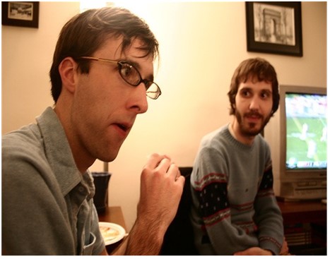
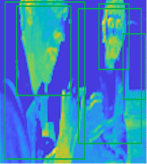
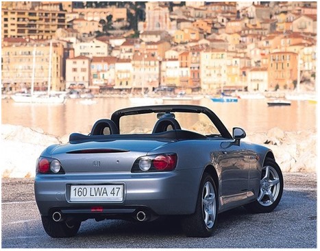
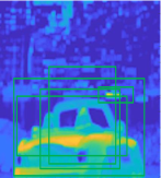
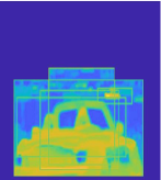
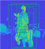
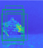
Effectiveness of Var_Inf We explore the effectiveness of the Var_Inf module by adding the module to Base+ID_LCM. It can be observed from Table 3 and Table 4 that the Var_Inf module also improves the performance. For ROIs extracted from each image, Base+ID_LCM thinks that all ROIs have the same importance and the contribution to multi-label classification is the same. However, because some regions may contain useful objects and some regions may be noise, if we treat them equally, those useless noise information will disturb our final classification results. Thus, we need to enhance those useful areas and suppress those noise areas. As shown in Figure 3, in this process, some of detected regions contains target objects, and some detect background information. However, after the regions are processed by this Var_Inf module, the features of regions containing target objects are enhanced and their colors become more prominent and striking. By considering their complex distribution, we apply the Var_Inf module to learn adaptive scaling factors that are used to weight ROIs. For weighted ROIs, more useful information will be sent to the later network, and that useless information will be blocked.
| Methods | mAP | CP | CR | CF1 | OP | OR | OF1 |
|---|---|---|---|---|---|---|---|
| Com_Sco | 84.5 | 75.4 | 81.4 | 78.3 | 79.9 | 84.3 | 82.0 |
| Base | 93.0 | 85.9 | 86.1 | 86.0 | 84.7 | 89.3 | 86.9 |
| Base+ Com_Sco | 93.8 | 87.3 | 87.1 | 87.2 | 87.7 | 89.9 | 88.8 |
| Methods | mAP | CP | CR | CF1 | OP | OR | OF1 |
|---|---|---|---|---|---|---|---|
| Com_Sco | 68.3 | 57.8 | 68.4 | 62.7 | 64.3 | 74.0 | 68.8 |
| Base | 82.9 | 83.7 | 72.7 | 77.9 | 84.5 | 76.2 | 80.1 |
| Base+ Com_Sco | 84.5 | 86.5 | 73.7 | 79.6 | 87.1 | 77.4 | 82.0 |
Effectiveness of Com_Sco We add the module Com_Sco to Base+ID_LCM+Var_Inf for demonstrating the effectiveness of Com_Sco module. As shown in Table 3 and Table 4, the results of comparison demonstrate its effectiveness. After obtaining the rough scores of each region on all labels, we think that score as a measure of the correlation between regions and labels can be viewed as a type of feature in label space. Since there is a correlation among labels, there should also be a correlation among regions. We view each region as a node and explore the correlation. In other words, we use the fused LCM to model a more accurate label distribution of this image instance. This module can make an effective supplement for the ResNet branch. In addition, in order to further prove the effectiveness of Com_Sco, we do more comparative experiments. Three cases are test respectively. Firstly, we only test the region-based branch without the Var_Inf module and the ID_LCM module. We use the individual LCM as the adjacent matrix. Secondly, we only test the global branch without the Var_Inf module, the ID_LCM and the Com_Sco module. The branch use the statistical LCM as the adjacent matrix. Thirdly, we use the fused branch without the Var_Inf module and the the ID_LCM module. They use the statistical LCM and the individual LCM as their adjacent matrixs respectively. The results in Table 5 and Table 6 further demonstrate its effectiveness. Although the performance of the Com_Sco module itself is not very good, it can be used as an effective supplement to the global branch to further improve the performance.
5. Conclusion
How to explore label dependencies is crucial for multi-label recognition task. In order to better model the correlation among labels, we propose an IA-GCNN model which involves a global branch modeling the whole image and a region-based branch exploring dependencies among ROIs. We first fuse both the statistical LCM and an individual one of each image instance that is constructed by mining the label dependencies based on the features of detected ROIs, and then inject adaptive information of label-awareness into the learned features of the model for label diffusion of instance-awareness in graph convolution. Simultaneously, considering the contribution differences of ROIs to multi-label classification, we introduce variational inference to learn adaptive scaling factors for those ROIs by considering their complex distribution. Experiments on MS-COCO and VOC datasets demonstrate the superiority of our proposed model.
References
- (1)
- Alemi et al. (2016) Alexander A. Alemi, Ian C Fischer, Joshua V. Dillon, and Kevin Murphy. 2016. Deep Variational Information Bottleneck. ArXiv abs/1612.00410 (2016).
- Barber and Agakov (2003) David Barber and Felix V. Agakov. 2003. The IM Algorithm: A Variational Approach to Information Maximization. In NIPS.
- Boutell et al. (2004) Matthew R. Boutell, Jiebo Luo, Xipeng Shen, and Christopher M. Brown. 2004. Learning multi-label scene classification. Pattern Recognit. 37 (2004), 1757–1771.
- Chalk et al. (2016) Matthew Chalk, Olivier Marre, and Gasper Tkacik. 2016. Relevant sparse codes with variational information bottleneck. In NIPS.
- Chen et al. (2018) Tianshui Chen, Zhouxia Wang, Guanbin Li, and Liang Lin. 2018. Recurrent Attentional Reinforcement Learning for Multi-label Image Recognition. In AAAI.
- Chen et al. (2019) Zhao-Min Chen, Xiu-Shen Wei, Peng Wang, and Yanwen Guo. 2019. Multi-Label Image Recognition With Graph Convolutional Networks. 2019 IEEE/CVF Conference on Computer Vision and Pattern Recognition (CVPR) (2019), 5172–5181.
- Deng et al. (2009) Jia Deng, Wei Dong, Richard Socher, Li-Jia Li, Kai Li, and Fei-Fei Li. 2009. ImageNet: A large-scale hierarchical image database. 2009 IEEE Conference on Computer Vision and Pattern Recognition (2009), 248–255.
- Everingham et al. (2009) Mark Everingham, Luc Van Gool, Christopher K. I. Williams, John M. Winn, and Andrew Zisserman. 2009. The Pascal Visual Object Classes (VOC) Challenge. International Journal of Computer Vision 88 (2009), 303–338.
- Ge et al. (2018b) Weifeng Ge, Sibei Yang, and Yizhou Yu. 2018b. Multi-evidence Filtering and Fusion for Multi-label Classification, Object Detection and Semantic Segmentation Based on Weakly Supervised Learning. 2018 IEEE/CVF Conference on Computer Vision and Pattern Recognition (2018), 1277–1286.
- Ge et al. (2018a) Zongyuan Ge, Dwarikanath Mahapatra, Suman Sedai, Rahil Garnavi, and Rajib Chakravorty. 2018a. Chest X-rays Classification: A Multi-Label and Fine-Grained Problem. ArXiv abs/1807.07247 (2018).
- Gong et al. (2013) Yunchao Gong, Yangqing Jia, Thomas Leung, Alexander Toshev, and Sergey Ioffe. 2013. Deep Convolutional Ranking for Multilabel Image Annotation. CoRR abs/1312.4894 (2013).
- Guillaumin et al. (2009) Matthieu Guillaumin, Thomas Mensink, Jakob J. Verbeek, and Cordelia Schmid. 2009. TagProp: Discriminative metric learning in nearest neighbor models for image auto-annotation. 2009 IEEE 12th International Conference on Computer Vision (2009), 309–316.
- He et al. (2016) Kaiming He, Xiangyu Zhang, Shaoqing Ren, and Jian Sun. 2016. Deep Residual Learning for Image Recognition. 2016 IEEE Conference on Computer Vision and Pattern Recognition (CVPR) (2016), 770–778.
- Huang et al. (2017) Gao Huang, Zhuang Liu, and Kilian Q. Weinberger. 2017. Densely Connected Convolutional Networks. 2017 IEEE Conference on Computer Vision and Pattern Recognition (CVPR) (2017), 2261–2269.
- Kingma and Welling (2014) Diederik P. Kingma and Max Welling. 2014. Auto-Encoding Variational Bayes. CoRR abs/1312.6114 (2014).
- Kipf and Welling (2017) Thomas Kipf and Max Welling. 2017. Semi-Supervised Classification with Graph Convolutional Networks. ArXiv abs/1609.02907 (2017).
- Lee et al. (2018) Chung-Wei Lee, Wei Fang, Chih-Kuan Yeh, and Yu-Chiang Frank Wang. 2018. Multi-label Zero-Shot Learning with Structured Knowledge Graphs. 2018 IEEE/CVF Conference on Computer Vision and Pattern Recognition (2018), 1576–1585.
- Li et al. (2016b) Qiang Li, Maoying Qiao, Wei Bian, and Dacheng Tao. 2016b. Conditional Graphical Lasso for Multi-label Image Classification. 2016 IEEE Conference on Computer Vision and Pattern Recognition (CVPR) (2016), 2977–2986.
- Li et al. (2014) Xin Li, Feipeng Zhao, and Yuhong Guo. 2014. Multi-label Image Classification with A Probabilistic Label Enhancement Model. In UAI.
- Li et al. (2016a) Yining Li, Chen Huang, Chen Change Loy, and Xiaoou Tang. 2016a. Human Attribute Recognition by Deep Hierarchical Contexts. In ECCV.
- Lin et al. (2014) Tsung-Yi Lin, Michael Maire, Serge J. Belongie, James Hays, Pietro Perona, Deva Ramanan, Piotr Dollár, and C. Lawrence Zitnick. 2014. Microsoft COCO: Common Objects in Context. ArXiv abs/1405.0312 (2014).
- Mohamed and Rezende (2015) Shakir Mohamed and Danilo Jimenez Rezende. 2015. Variational Information Maximisation for Intrinsically Motivated Reinforcement Learning. In NIPS.
- Pennington et al. (2014) Jeffrey Pennington, Richard Socher, and Christopher D. Manning. 2014. Glove: Global Vectors for Word Representation. In EMNLP.
- Ren et al. (2015) Shaoqing Ren, Kaiming He, Ross B. Girshick, and Jian Sun. 2015. Faster R-CNN: Towards Real-Time Object Detection with Region Proposal Networks. IEEE Transactions on Pattern Analysis and Machine Intelligence 39 (2015), 1137–1149.
- Simonyan and Zisserman (2015) Karen Simonyan and Andrew Zisserman. 2015. Very Deep Convolutional Networks for Large-Scale Image Recognition. CoRR abs/1409.1556 (2015).
- Szegedy et al. (2016) Christian Szegedy, Vincent Vanhoucke, Sergey Ioffe, Jon Shlens, and Zbigniew Wojna. 2016. Rethinking the Inception Architecture for Computer Vision. 2016 IEEE Conference on Computer Vision and Pattern Recognition (CVPR) (2016), 2818–2826.
- Tsoumakas and Katakis (2007) Grigorios Tsoumakas and Ioannis Katakis. 2007. Multi-Label Classification: An Overview. IJDWM 3 (2007), 1–13.
- Wang et al. (2016) Jiang Wang, Yi Yang, Junhua Mao, Zhiheng Huang, Chang Huang, and Wei Xu. 2016. CNN-RNN: A Unified Framework for Multi-label Image Classification. 2016 IEEE Conference on Computer Vision and Pattern Recognition (CVPR) (2016), 2285–2294.
- Wang et al. (2020) Ya Wang, Dongliang He, Fu Li, Xiang Long, Zhichao Zhou, Jinwen Ma, and Shilei Wen. 2020. Multi-Label Classification with Label Graph Superimposing. ArXiv abs/1911.09243 (2020).
- Wang et al. (2017) Zhouxia Wang, Tianshui Chen, Guanbin Li, Ruijia Xu, and Liang Lin. 2017. Multi-label Image Recognition by Recurrently Discovering Attentional Regions. 2017 IEEE International Conference on Computer Vision (ICCV) (2017), 464–472.
- Wei et al. (2016) Yunchao Wei, Wei Xia, Min Lin, Junshi Huang, Bingbing Ni, Jian Dong, Yao Zhao, and Shuicheng Yan. 2016. HCP: A Flexible CNN Framework for Multi-Label Image Classification. IEEE Transactions on Pattern Analysis and Machine Intelligence 38 (2016), 1901–1907.
- Yang et al. (2016) H. T. Yang, Joey Tianyi Zhou, Yu Lin Zhang, Bin-Bin Gao, Jianxin Wu, and Jianfei Cai. 2016. Exploit Bounding Box Annotations for Multi-Label Object Recognition. 2016 IEEE Conference on Computer Vision and Pattern Recognition (CVPR) (2016), 280–288.
- Zhang et al. (2018) Junjie Zhang, Qi Wu, Chunhua Shen, J. Andrew Zhang, and Jianfeng Lu. 2018. Multilabel Image Classification With Regional Latent Semantic Dependencies. IEEE Transactions on Multimedia 20 (2018), 2801–2813.
- Zhu et al. (2017) Feng Zhu, Hongsheng Li, Wanli Ouyang, Nenghai Yu, and Xiaogang Wang. 2017. Learning Spatial Regularization with Image-Level Supervisions for Multi-label Image Classification. 2017 IEEE Conference on Computer Vision and Pattern Recognition (CVPR) (2017), 2027–2036.