Elimination of the Blue Loops in the Evolution of Intermediate-mass Stars by the Neutrino Magnetic Moment and Large Extra Dimensions

Abstract

For searching beyond Standard Model physics, stars are laboratories which complement terrestrial experiments. Massless neutrinos in the Standard Model of particle physics cannot have a magnetic moment, but massive neutrinos have a finite magnetic moment in the minimal extension of the Standard Model. Large extra dimensions are a possible solution of the hierarchy problem. Both of these provide additional energy loss channels in stellar interiors via the electromagnetic interaction and radiation into extra dimensions, respectively, and thus affect stellar evolution. We perform simulations of stellar evolution with such additional energy losses and find that they eliminate the blue loops in the evolution of intermediate-mass stars. The existence of Cepheid stars can be used to constrain the neutrino magnetic moment and large extra dimensions. In order for Cepheids to exist, the neutrino magnetic moment should be smaller than the range $\sim 2\times 10^{-10}$ to $4\times 10^{-11}\mu_{\mathrm{B}}$ , where $\mu_{\mathrm{B}}$ is the Bohr magneton, and the fundamental scale in the (4+2)-spacetime should be larger than $\sim 2$ to 5 TeV, depending on the rate of the ¹²C$(\alpha,\gamma)^{16}$O reaction. The fundamental scale also has strong dependence on the metallicity. This value of the magnetic moment is in the range explored in the reactor experiments, but higher than the limit inferred from globular clusters. Similarly the fundamental scale value we constrain corresponds to a size of the compactified dimensions comparable to those explored in the torsion balance experiments, but is smaller than the limits inferred from collider experiments and low-mass stars.

1 Introduction

Intermediate-mass stars deviate from the red giant branch and form a loop towards the blue region in the Hertzsprung-Russell (HR) diagram during central helium burning (Kippenhahn, Weigert & Weiss, 2012). Such a loop is called a “blue loop.” Stars spend considerable time on the blue loop, so many blue giants have been discovered (e.g. McQuinn et al., 2011; Dohm-Palmer & Skillman, 2002; Evans, 1993). The blue loops can cross the Cepheid instability strip if their endpoint extend to high enough temperature. In that case, the stars on the blue loops are observed as Cepheid variables.

Stars have been used to explore beyond-standard physics which may be difficult to reach with laboratory experiments (Raffelt, 1996). Recently, it was pointed out that the blue loops in the evolution of intermediate-mass stars can be eliminated if energy loss from axion emission (Friedland, Giannotti & Wise, 2013) is included in stellar evolution calculations. Because the blue loops are a ubiquitous characteristic of blue giants and Cepheid variables, this is a powerful way to relate new physics to observations. We apply this idea to the exploration of non-standard energy losses that originate from the neutrino magnetic moment ($\mu_{\nu}$; NMM) and large extra dimensions (LEDs).

In the standard model (SM) of particle physics, neutrinos are assumed to be massless. However, neutrino oscillation observations have revealed that they have mass eigenstates (e.g. Fukuda et al., 1998). The NMM is allowed only for massive neutrinos and the minimally extended SM predicts a small but finite magnetic moment (Shrock, 1982; Fujikawa & Shrock, 1980).

Since the NMM is a key to physics beyond the Standard Model, several experiments have been performed to find it and determine its magnitude (Balantekin & Kayser, 2018; Giunti & Studenikin, 2015). The most recent constraint comes from the GEMMA experiment (Beda et al., 2013), which measures the scattering cross sections of electrons and reactor anti-electron neutrinos. This constrains the magnetic moment at $\mu_{\nu}<2.9\times 10^{-11}\mu_{\mathrm{B}}$ (90% C.L.).

In addition to the intermediate-mass stars considered here NMMs can also be constrained from low-mass stars. The luminosity of the tip of red giant branch is sensitive to the energy loss. Theoretical luminosities are compared to the color-magnitude diagram of globular clusters (Arceo-Díaz et al., 2015; Viaux et al., 2013a, b; Raffelt & Weiss, 1992) and a stringent constraint, $\mu_{\nu}<2.2\times 10^{-12}\mu_{\mathrm{B}}$, is reported (Arceo-Díaz et al., 2015).

The idea of LEDs is proposed by Arkani-Hamed, Dimopoulos & Dvali (1998) to solve the hierarchy problem, i.e. the huge difference between the electroweak scale $\sim$ TeV and the Planck scale $\sim 10^{16}$ TeV (Tanabashi et al., 2018). The Planck mass $M_{\mathrm{S}}$ in the $(4+n)$-dimensional spacetime is related with that $M_{\mathrm{P}}$ in the 4-dimensional spacetime as (Barger et al., 1999)

$$M_{\mathrm{P}}^{2}=\Omega_{n}R^{n}M_{\mathrm{S}}^{n+2},$$ (1)

where $R$ is the size of the compactified dimensions and $\Omega_{n}$ is a numerical factor which depends on the geometry of compactification. For example for a torus $\Omega_{n}=(2\pi)^{n}$. In order for the hierarchy problem to be solved, $M_{\mathrm{S}}$ should coincide with the electroweak scale. For the $n=1$ model, this requires $R\sim 10^{10}$ km, which is clearly excluded by the inverse-square law on the scale of the Solar System. In this study, therefore, we focus on the simplest possible case of $n\geq 2$.

The most direct probes of extra dimensions come from torsion balance experiments (Murata & Tanaka, 2015; Adelberger et al., 2009) which measure gravitation at the sub-millimeter range. The gravitational field between two masses $m_{1}$ and $m_{2}$ is often parametrized by the Yukawa potential

$$V(r)=-G\frac{m_{1}m_{2}}{r}\left(1+\alpha e^{-r/R}\right).$$ (2)

The $n=2$ model corresponds to $\alpha=16/3$. The most recent torsion experiments report $R\leq 37\;\mu\mathrm{m}$ (Tan et al., 2020) and $R<30\;\mu\mathrm{m}$ (Lee et al., 2020). For $n=2$ this corresponds to a limit of $M_{\mathrm{S}}\gtrsim 3$ TeV. For $n=3$ this corresponds to a lower limit on $M_{\mathrm{S}}$ which is well below the electroweak scale.

Hadron colliders have also been used to search for gravitons. These cannot be directly detected, so energetic jets are examined for missing transverse energy. From this, the value of $M_{\mathrm{D}}$ is extracted, where $M_{\mathrm{D}}$ is defined as

$$M_{\mathrm{P}}^{2}=R^{n}M_{\mathrm{D}}^{n+2}.$$ (3)

The Compact Muon Solenoid (CMS) experiment at the Large Hadron Collider reports $M_{\mathrm{D}}>9.9$ TeV for $n=2$ (Sirunyan et al., 2018). This corresponds to a limit of $M_{\mathrm{S}}\gtrsim 3.9$ TeV. The corresponding limits from the ATLAS collaboration are slightly lower (Aaboud et al., 2018).

A more stringent bound comes from $\gamma$-ray fluxes from neutron stars (Fermi-LAT Collaboration et al., 2012; Hannestad & Raffelt, 2003). A recent observation by the Fermi Large Area Telescope reports a constraint $R<9.5$ nm for the $n=2$ model (Fermi-LAT Collaboration et al., 2012).

Stellar evolution calculations have shown that the tip of the red giant branch is sensitive to LEDs. Cassisi et al. (2000) conclude that $M_{\mathrm{S}}>3$ TeV by comparing stars in globular clusters and theoretical stellar evolution. This value is similar to the experimental bounds coming from collider and torsion experiments. Both types of experiments – with very different systematic errors – yield bounds in $M_{\mathrm{S}}$ that are comparable to those derived from evaluations of the tip of the red giant branch.

Similarly, bounds on neutrino magnetic moments obtained from arguments of energy-loss in low-mass stars are within an order of magnitude of the experimental bounds. Terrestrial experiments looking for extra dimensions, such as the torsion balance experiments, and those looking for neutrino magnetic moments are reaching their limits of exploration. To improve the limits on the inverse square law requires a significant increase in the background-free sensitivity for the torsion balance experiments which will be rather difficult. To improve the limits on the neutrino magnetic moment requires ability to measure an exceedingly small amount of the electron recoil energy. Limits from both kind of terrestrial experiments are subject to very different systematic errors as compared to the limits from low-mass stars. Hence it is desirable to explore if other astronomical testbeds can yield limits subject to different systematic errors. In this paper we explore bounds obtained from considerations of evolution of intermediate mass stars in the ”blue loop” epoch as these would be subject to different uncertainties than the low-mass stars.

This paper is organized as follows. Section 2 describes the treatment of the extra energy loss due to NMMs and LEDs in stellar models. Section 3 describes the results of stellar evolution calculations. In Section 4, we summarize and discuss the constraints achieved in this study.

2 Method

2.1 Energy Loss by the Neutrino Magnetic Moment

For a non-zero NMM, the neutrino energy loss increases because of an additional electromagnetic contribution to the neutrino emissivity. Here we consider two processes: plasmon decay ($\gamma\rightarrow\nu\bar{\nu}$) and neutrino pair production ($e^{+}e^{-}\rightarrow\nu\bar{\nu}$). The additional energy loss rate due to plasmon decay is given as (Heger et al., 2009; Haft, Raffelt & Weiss, 1994)

$$\epsilon^{\mu}_{\mathrm{plas}}=0.318\left(\frac{\omega_{\mathrm{pl}}}{10\;\mathrm{keV}}\right)^{-2}\left(\frac{\mu_{\nu}}{10^{-12}\mu_{\mathrm{B}}}\right)^{2}\epsilon_{\mathrm{plas}},$$ (4)

where $\epsilon_{\mathrm{plas}}$ is the standard energy loss (Itoh et al., 1996) and $\omega_{\mathrm{pl}}$ is the plasma frequency (Raffelt, 1996)

$$\omega_{\mathrm{pl}}=28.7\;\mathrm{eV}\frac{(Y_{\mathrm{e}}\rho)^{\frac{1}{2}}}{(1+(1.019\times 10^{-6}Y_{\mathrm{e}}\rho)^{\frac{2}{3}})^{\frac{1}{4}}}.$$ (5)

Here $Y_{\mathrm{e}}$ is the electron fraction and $\rho$ is the density in units of $\mathrm{g\;cm^{-3}}$. The additional energy loss rate due to pair production is written as (Heger et al., 2009)

$$\epsilon^{\mu}_{\mathrm{pair}}=1.6\times 10^{11}\;\mathrm{erg\;g^{-1}\;s^{-1}}\left(\frac{\mu_{\nu}}{10^{-10}\mu_{\mathrm{B}}}\right)^{2}\frac{e^{-\frac{118.5}{T_{8}}}}{\rho_{4}},$$ (6)

where $T_{8}=T/(10^{8}\;\mathrm{K})$ and $\rho_{4}=\rho/(10^{4}\;\mathrm{g\;cm^{-3}})$.

2.2 Energy Loss by Large Extra Dimensions

A possible existence of compactified extra dimensions results in Kaluza-Klein (KK) modes of gravitons $G_{\mathrm{KK}}$ with mass $m^{2}_{\bm{n}}={\bm{n}}^{2}/R^{2}$, where $\bm{n}$ is the index for the $n^{th}$ KK modes. The KK gravitons can radiate into extra dimensions and thus work as an additional source of the energy loss, while standard model particles are confined to the 4-dimensional subspace. We consider three processes: photon-photon annihilation ($\gamma\gamma\rightarrow G_{\mathrm{KK}}$), gravi-Compton-Primakoff scattering ($e^{-}\gamma\rightarrow e^{-}G_{\mathrm{KK}}$) and gravi-bremsstrahlung ($e^{-}(Ze)\rightarrow e^{-}(Ze)G_{\mathrm{KK}}$).

The numerical formulae for these processes are given in Hansen et al. (2015) and Barger et al. (1999). The energy loss rates for photon-photon annihilation, gravi-Compton-Primakoff scattering and gravi-bremsstrahlung in the nondegenerate condition are given by

$$\epsilon_{\gamma\gamma}=5.1\times 10^{-9}T^{9}_{7}\rho^{-1}_{6}\left(\frac{M_{\mathrm{S}}c^{2}}{1\;\mathrm{TeV}}\right)^{-4}\;{\mathrm{erg\;g^{-1}\;s^{-1}}},$$ (7)

$$\epsilon_{\mathrm{GCP}}=4.5\times 10^{-6}T^{7}_{7}\left(\frac{M_{\mathrm{S}}c^{2}}{1\;\mathrm{TeV}}\right)^{-4}\;{\mathrm{erg\;g^{-1}\;s^{-1}}},$$ (8)

$$\epsilon_{\mathrm{GB}}=5.8\times 10^{-3}\bar{Z}^{2}_{7}T^{3}_{7}\left(\frac{M_{\mathrm{S}}c^{2}}{1\;\mathrm{TeV}}\right)^{-4}\;{\mathrm{erg\;g^{-1}\;s^{-1}}},$$ (9)

respectively. Here $\bar{Z}_{7}$ is the mean ion charge relative to nitrogen, $T_{7}=T/(10^{7}\;\mathrm{K})$ and $\rho_{6}=\rho/(10^{6}\;\mathrm{g\;cm^{-3}})$.

2.3 Stellar Model

We use a one-dimensional stellar evolution code Modules for Experiments in Stellar Astrophysics (MESA; Paxton et al., 2011, 2013, 2015, 2018, 2019) version 10398. The code adopts the equation of state of Rogers & Nayfonov (2002) and Timmes & Swesty (2000) and opacities of Iglesias & Rogers (1996, 1993) and Ferguson et al. (2005). Nuclear reaction rates are taken from NACRE (Angulo et al., 1999) with weak rates from Langanke & Martínez-Pinedo (2000); Oda et al. (1994); Fuller, Fowler & Newman (1985). The prescription for screening is based on Alastuey & Jancovici (1978) and Itoh et al. (1979).

The initial composition adopted in our models is based on the solar system abundances. Conventionally, the standard solar metallicity has been $Z=0.02$ (Anders & Grevesse, 1989). However, recent literature shows lower metallicities of $Z=0.0122$ (Asplund, Grevesse & Sauval, 2005), 0.0134 (Asplund et al., 2009) and 0.0148 (Lodders, 2020). In our models, we adopt two compositions: $(Y,\;Z)=(0.28,\;0.02)$ from Anders & Grevesse (1989) and $(Y,\;Z)=(0.2463,\;0.0148)$ from Asplund et al. (2009). We call these models Case A and Case B, respectively (Table 1).

	X	Y	Z
Case A	0.70	0.28	0.02
Case B	0.7389	0.2463	0.0148

Table 1: The initial composition adopted in our models.

Convective mixing lengths are fixed to $\alpha=1.6$, which were adopted in Friedland, Giannotti & Wise (2013). The overshoot parameter is set to be $f_{\mathrm{ov}}=0.005$. When the effective temperature $T_{\mathrm{eff}}$ is lower than $10^{4}$ K, the mass loss table compiled by de Jager, Nieuwenhuijzen & van der Hucht (1988) is used. When $T_{\mathrm{eff}}$ is higher than $10^{4}$ K, mass loss is not taken into account. Pulsation-driven mass loss (Neilson, Cantiello & Langer, 2011; Neilson & Lester, 2008) within the Cepheid instability strip is not considered. The nuclear reaction network includes 22 nuclides (approx21_plus_co56.net). Evolution is followed until the end of core helium burning.

3 Results

We calculate non-rotating stellar models with 7, 8, 9, and 10$M_{\odot}$. The adopted NMM is $\mu_{12}=100$, 200 and 300, where $\mu_{12}$ is the neutrino magnetic moment in units of $10^{-12}\mu_{B}$ , and the LED adopted mass scales are $M_{\mathrm{S}}=3$, 2, and 1 TeV. In Section 3.1, we show the HR diagrams of these models. In Section 3.2, we discuss the evolution of the helium burning core and contribution of each elementary process to the energy loss.

3.1 Elimination of the Blue Loops

3.1.1 Case A

The upper panel in Fig. 1 is the HR diagram for the standard case. In this case, all of the models with 7-10$M_{\odot}$ show the blue loops. The loops in this mass range cross the Cepheid instability strip, in which stars pulsate as Cepheid variables.

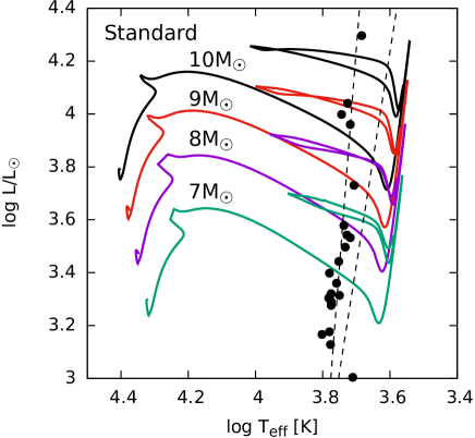
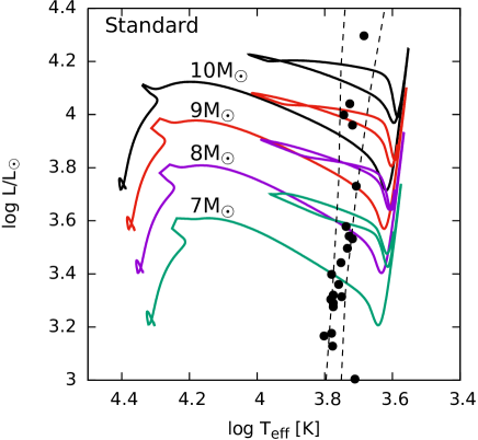
Figure 1: The HR diagram with standard physics. The upper panel shows the models with $Z=0.02$ (i.e. Case A) and the lower shows the models with $Z=0.0148$ (i.e. Case B). The broken lines indicate the edges of the instability strip in models. The $Z=0.02$ models in Bono, Castellani & Marconi (2000a) are adopted for Case A and the $Z=0.014$ model in Anderson et al. (2016) is adopted in Case B. The points are samples of Galactic Cepheids reported in Turner & Burke (2002).

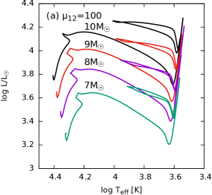
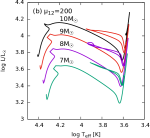
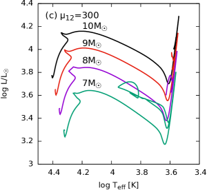
Figure 2: The HR diagram with the NMMs of (a) $\mu_{12}=100$, (b) $\mu_{12}=200$ and (c) $\mu_{12}=300$ in Case A.

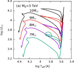
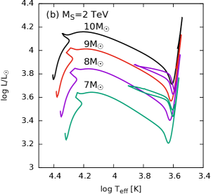
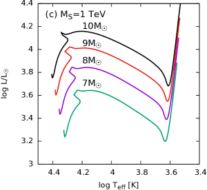
Figure 3: The HR diagram with LED of (a) $M_{\mathrm{S}}=3$ TeV, (b) $M_{\mathrm{S}}=2$ TeV and (c) $M_{\mathrm{S}}=1$ TeV in Case A.

Fig. 2 is the HR diagram of stars with NMMs of $\mu_{12}=100$, 200 and 300. Though the morphology of the blue loops does not change when $\mu_{12}=100$, in the case of $\mu_{12}=200$, the loop is eliminated for the $10M_{\odot}$ star. When the NMM is as large as $\mu_{12}=300$, only the $7M_{\odot}$ model exhibits a blue loop, while its morphology is significantly affected.

Fig. 3 shows HR diagrams of stars with LEDs of $M_{\mathrm{S}}=3$, 2 and 1 TeV. It is seen that, when $M_{\mathrm{S}}=3$ TeV, the blue loops remain in all of the models, but the morphology is affected for the $7M_{\odot}$ model. In the case of $M_{\mathrm{S}}=2$ TeV, the loop is eliminated for the $10M_{\odot}$ and $9M_{\odot}$ stars. When $M_{\mathrm{S}}=1$ TeV, the blue loops are eliminated for all of the models.

Although the blue loops do not disappear for $\mu_{12}=100$ and $M_{\mathrm{S}}=3$ TeV, the duration, $t_{\mathrm{BG}}$, of the blue giant phase becomes shorter because of the additional energy loss. Fig. 4 shows the evolution of the effective temperature as a function of the stellar age for these cases. The upper panel shows the result for various assumptions of the NMM and the lower panel shows the result for various assumptions of LED sizes. The sudden expansion at $\sim 21.5$ Myr is the Hertzsprung gap, where the helium core contracts rapidly and the envelope expands (Kippenhahn, Weigert & Weiss, 2012; Sandage & Schwarzschild, 1952). The bump around $\sim 23.5$ Myr corresponds to the blue loop. It is seen that $t_{\mathrm{BG}}=0.64$ Myr in the standard case, while $t_{\mathrm{BG}}=0.55$ Myr when $\mu_{12}=100$ and $t_{\mathrm{BG}}=0.35$ Myr when $M_{\mathrm{S}}=3$ TeV. This difference is potentially observable from the ratio of blue and red giants (McQuinn et al., 2011; Dohm-Palmer & Skillman, 2002).

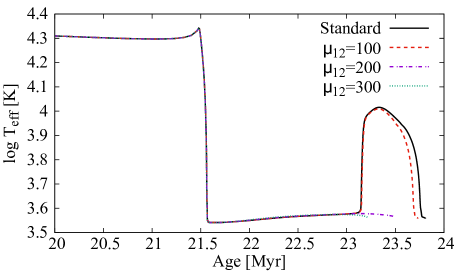
Figure 4: The time evolution of the effective temperature for the $10M_{\odot}$ models in Case A. The upper panel shows the effect of the NMM and the lower panel shows the effect of LED.

3.1.2 Case B

The HR diagram in the standard case is shown in the lower panel of Fig. 1. The blue loops appear in all of the models with 7-10$M_{\odot}$. The edges of the blue loops are bluer than those in Case A.

Fig. 5 is the HR diagram with NMMs of $\mu_{12}=100$, 200 and 300. The blue loops remain in the case of $\mu_{12}=100$, while they are eliminated in the $10M_{\odot}$ model when $\mu_{12}=200$ and in all of the 7, 8, 9 and $10M_{\odot}$ models when $\mu_{12}=300$.

Fig. 6 is the HR diagram with LEDs of $M_{\mathrm{S}}=3$, 2 and 1 TeV. Contrary to the result in Case A, the blue loop in the $10M_{\odot}$ model is eliminated even when $M_{\mathrm{S}}=1$ TeV. The blue loop only in $7M_{\odot}$ model survives when when $M_{\mathrm{S}}=2$ TeV and all of the loops are eliminated when $M_{\mathrm{S}}=3$ TeV.

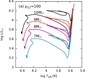
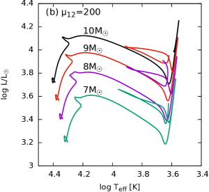
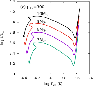
Figure 5: The HR diagram with LED of (a) $\mu_{12}=100$, (b) $\mu_{12}=200$ and (c) $\mu_{12}=300$ in Case B.

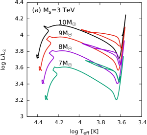
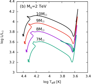
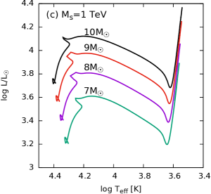
Figure 6: The HR diagram with LED of (a) $M_{\mathrm{S}}=3$ TeV, (b) $M_{\mathrm{S}}=2$ TeV and (c) $M_{\mathrm{S}}=1$ TeV in Case B.

3.2 Evolution of the Core

Fig. 7 shows the central temperature and density evolution for stars of various mass. The upper panel shows the result with an assumed NMM of $\mu_{12}=200$ and the lower panel shows the result with LED of $M_{\mathrm{S}}=2$ TeV. The grey contour shows the enhancement factor, $\log f$, of the energy loss defined as

$$\log f=\log\left(\frac{\epsilon_{\nu}+\epsilon_{\mathrm{extra}}}{\epsilon_{\nu}}\right),$$ (10)

where $\epsilon_{\nu}$ is the standard energy loss and $\epsilon_{\mathrm{extra}}$ is the additional energy loss caused by the NMM of $\mu_{12}=200$ and LED of $M_{\mathrm{S}}=2$ TeV. It is seen that the energy loss rate is enhanced by $10^{2}$-$10^{4}$ times.

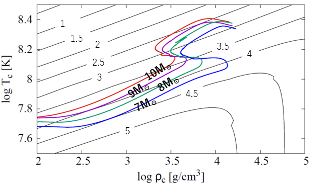
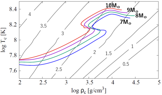
Figure 7: The evolution of the central temperature and density in Case A. The upper panel shows the effect of the NMM of $\mu_{12}=200$ and the lower panel shows the effect of LED of $M_{\mathrm{S}}=2$ TeV. The contour shows the enhancement factor $\log f$ defined in the text.

From Fig. 7, one sees that the contribution of $\epsilon_{\mathrm{extra}}$ decreases as a function of the temperature when $\mu_{12}=200$, while it increases when $M_{\mathrm{S}}=2$ TeV. This is explained in Fig. 8, which shows the energy loss rates of each elementary process at a density of $10^{4}$ g $\mathrm{cm^{-3}}$. The upper panel assumes an NMM of $\mu_{12}=200$ and the lower panel assumes a LED of $M_{\mathrm{S}}=2$ TeV. Here $\epsilon^{\mu}_{\mathrm{plas}},\;\epsilon^{\mu}_{\mathrm{pair}},\;\epsilon_{\gamma\gamma},\;\epsilon_{\mathrm{GCP}}$ and $\epsilon_{\mathrm{GB}}$ are defined in Section 2. The values of $\epsilon^{\mu}_{\mathrm{tot}}$ and $\epsilon^{\mathrm{KK}}_{\mathrm{tot}}$ are the total energy loss due to the NMM and LED, respectively. The values $\epsilon_{\mathrm{pair}},\;\epsilon_{\mathrm{plas}}$ and $\epsilon_{\mathrm{tot}}$ are the standard neutrino energy losses (Itoh et al., 1996). In the case of $\mu_{12}=200$, the dominant process at $\log T\sim 8.2$, where helium burning occurs, is plasmon decay. On the other hand, in the case of $M_{\mathrm{S}}=2$ TeV, the dominant process is photon-photon annihilation. The photoneutrino energy loss rate $\epsilon_{\mathrm{photo}}$ is proportional to $T^{8}$ (Petrosian, Beaudet & Salpeter, 1967), while the plasma energy loss rate $\epsilon^{\mu}_{\mathrm{plas}}$ is proportional to $T^{3}$ (Inman & Ruderman, 1964). This is the reason why $f$ becomes smaller in the hot region when $\mu_{12}=200$. On the other hand, the photon-photon annihilation rates $\epsilon_{\gamma\gamma}$ is proportional to $T^{9}$ (Barger et al., 1999), therefore $f$ is larger in the hot region when $M_{\mathrm{S}}=2$.

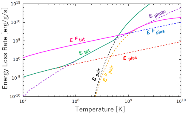
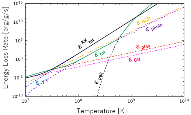
Figure 8: Different contributions to the energy loss rates at $\rho=10^{4}$ g $\mathrm{cm^{-3}}$. The upper panel shows the effect of the NMM of $\mu_{12}=200$ and the lower panel shows the effect of LED of $M_{\mathrm{S}}=2$ TeV.

The physical mechanism at the onset of the blue loops is still under debate (e.g. Kippenhahn, Weigert & Weiss, 2012; Xu & Li, 2004a). One possible mechanism is the so-called mirror reflection principle. When a star leaves the red giant branch to the blue loop, nuclear burning energy is used to expand the core (Choplin et al., 2017). Because of the mirror reflection principle, the expansion of the core leads to the contraction of the envelope and thus higher effective temperature. However, the NMM and LED extract energy from the core and prevent the expansion of the core. Therefore a star cannot start a detour to a blue giant.

Fig. 9 shows the evolution of the helium core radius with different NMMs. It is seen that the core radius $R_{\mathrm{He}}$ increases after $\sim 23.2$ Myr in the case of $\mu_{12}=0$ and 100, while it decreases when $\mu_{12}=200$ and 300. This is consistent with the explanation of the blue loop by the mirror reflection principle.

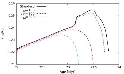
Figure 9: The radii of the helium core as a function of stellar age for the $10M_{\odot}$ models in Case A. The solid line shows the result without the NMM and the others show the results for $\mu_{12}=100,\;200$ and 300.

3.3 Effects of Reaction Rate Uncertainties

In the fiducial models, we adopt the NACRE reaction rates (Angulo et al., 1999). However, uncertainties in nuclear reaction rates can significantly affect morphology of the blue loops (Valle et al., 2009; Xu & Li, 2004a; Brunish & Becker, 1990) and thus the threshold of elimination of the loops. In this section, we study the effects of uncertainties in the triple-$\alpha$ and ¹²C$(\alpha,\;\gamma)^{16}$O reactions, which govern core helium burning.

3.3.1 Triple-$\alpha$ Reaction

NACRE estimates temperature-dependent uncertainties in the triple-$\alpha$ reaction to be $\lesssim 20\%$ at $\sim 10^{8}$ K. We adopt this uncertainties to study the sensitivity of the blue loops.

Fig. 10 shows the evolution of the $10M_{\sun}$ star with the triple-$\alpha$ reactions changed within the NACRE uncertainties. Although the loop extends to the slightly bluer region when the lower rate is adopted, morphology of the blue loops is not affected significantly by the different triple-$\alpha$ rates. This suggests that the threshold of elimination of the loops is robust against the present uncertainties.

Figure 10: The HR diagram of the $10M_{\odot}$ model with different triple-$\alpha$ reaction rates. The solid line adopts the NACRE standard reaction rate, while the broken lines adopt the higher and lower limits of the rate quoted in NACRE table. The initial composition is set to be Case B.

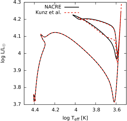
Figure 11: The HR diagram of the $10M_{\odot}$ model with different ¹²C$(\alpha,\;\gamma)^{16}$O reaction rates. The solid line adopts the NACRE standard reaction rate, while the broken line adopts the rate quoted in Kunz et al. (2002). The initial composition is set to be Case B.

3.3.2 ¹²C$(\alpha,\;\gamma)^{16}$O Reaction

The low-energy cross sections of the ¹²C$(\alpha,\;\gamma)^{16}$O reaction have not been measured yet (e.g. deBoer et al., 2017). Kunz et al. (2002) proposed lower reaction rates than NACRE compilation, based on their new measurements of E1- and E2-capture cross sections. Their reaction rates are $\sim 30\%$ smaller than the NACRE rate at $\sim 10^{8}$ K. We adopt the rate recommended by Kunz et al. (2002) to perform a sensitivity study.

Fig. 11 shows the evolution of the $10M_{\odot}$ model with the different ¹²C$(\alpha,\;\gamma)^{16}$O reaction rates. It is seen that the tip of the blue loop becomes redder when the Kunz et al. (2002) rate is adopted and the shape of the loops is significantly different around $\log T_{\mathrm{eff}}\sim 3.65$ between the two.

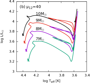
Figure 12: The HR diagram (a) without beyond Standard Model physics, (b) with $\mu_{12}=40$, and (c) with $M_{\mathrm{S}}=5$ TeV. The ¹²C$(\alpha,\;\gamma)^{16}$O rate is from Kunz et al. (2002). The initial composition is set to be Case B.

Fig. 12 shows the evolution of the 7-10$M_{\odot}$ stars with the ¹²C$(\alpha,\;\gamma)^{16}$O rate quoted in Kunz et al. (2002). When beyond-standard physics is not adopted, the tip of the blue loops becomes redder when reaction rate is lower, as reported in Valle et al. (2009) and Brunish & Becker (1990). Interestingly, the threshold of elimination of the loops is much lower than that with the NACRE rate. As shown in Fig. 12, the blue loops are suppressed in the $10M_{\odot}$ model when $\mu_{12}>40$ or $M_{\mathrm{S}}<5$ TeV with the rate in Kunz et al. (2002), while these thresholds are $\mu_{12}>200$ and $M_{\mathrm{S}}<3$ TeV for the NACRE rate, respectively, as has already been discussed in Figs. 2 - 6.

3.4 Effects on Heavier Cepheids

Some of Galactic Cepheid progenitors have been estimated (Turner, 1996) to be as massive as $\sim 20M_{\odot}$, using an empirical mass-period relation of Cepheids. Models of such a massive star do not undergo the blue loop during central helium burning (e.g. Anderson et al., 2016; Valle et al., 2009; Bono et al., 2000; Schaller et al., 1992). Less massive stars with $<15M_{\odot}$ cross the Hertzsprung gap so rapidly that there is little chance to observe those in the instability strip. However, massive stars with $>15M_{\odot}$ achieve the central temperature high enough to ignite helium burning before they reach the red giant branch. In this case, the time to cross the gap slows down, so it becomes more probable to observe them in the instability strip.

Fig. 13 shows evolution of the effective temperature for the $20M_{\odot}$ models in Case B. The black line shows the standard evolution and the purple and red lines adopt $\mu_{12}=100$ and $M_{\mathrm{S}}=3$ TeV, respectively. It is seen that the extra energy losses shorten the timescale of helium burning. The dots show crossing of the blue edge of the instability strip. Although validity of the extrapolation of the model edge (Bono, Castellani & Marconi, 2000a) to higher luminosities is uncertain, the stars spend 10-20 kyr in the instability strip even when $\mu_{12}=100$ or $M_{\mathrm{S}}=3$ TeV is adopted. Therefore these effects do not contradict the observed rare massive Cepheids.

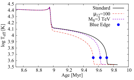
Figure 13: Time evolution of the effective temperature for the $20M_{\odot}$ models in Case B. The black line shows the standard model, and the purple and red lines adopt $\mu_{12}=100$ and $M_{\mathrm{S}}=3$ TeV, respectively. The dots represent crossing of the blue edge of the instability strip (Bono, Castellani & Marconi, 2000a).

3.5 Possible Effects of Mass Loss and Rotation

The purpose of this paper is to show fiducial models of intermediate-mass stars with physics beyond the SM, so exhaustive evaluation of theoretical uncertainties is out of its scope. However, the evolution of intermediate-mass stars is sensitive to other physical processes, which is the very reason why they can potentially used as a probe of new physics.

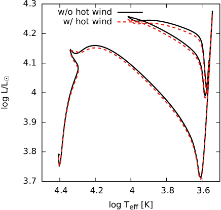
Figure 14: The HR diagram for the $10M_{\odot}$ models with standard physics in Case A. The solid line shows the model without mass loss on the MS, while the broken line shows the model with it.

In our models, the treatment of mass loss in the red supergiant phase and the blue loop is based on de Jager, Nieuwenhuijzen & van der Hucht (1988), which covers the temperature and the luminosity ranges we are interested in. This mass loss rate on the main sequence (MS) is not considered because it is as small as $10^{-8}$-$10^{-9}M_{\odot}$ /yr (de Jager, Nieuwenhuijzen & van der Hucht, 1988). Figure 14 shows the comparison between the $10M_{\odot}$ models with and without mass loss during the MS. The solid line shows the fiducial model which was also shown in Fig. 1 and the broken line shows the model with the additional mass loss based on de Jager, Nieuwenhuijzen & van der Hucht (1988). It is seen that the mass loss during the MS slightly decreases the luminosity of the blue loop. The effect of the mass loss on the MS on morphology of the blue loops is moderate and thus is not a major source of uncertainties.

It has been pointed out that shocks generated by the pulsation drive mass loss up to $10^{-7}M_{\odot}$ /yr (Neilson & Lester, 2008). Because of such pulsation-driven mass loss, Cepheid variables can lose 5-10 % of their mass (Neilson, Cantiello & Langer, 2011). Morphology of the blue loops can be significantly affected by pulsation-driven mass loss, so it is desirable to study uncertainties that originate from it.

Effects of rotation are not included in our models. However, the typical rotational velocity of B-stars on the MS with 5-9$M_{\odot}$ is as high as 10-30 % of the critical velocity (Huang, Gies & McSwain, 2010), so it is important to study the rotational effect. Rotation makes the blue loops more luminous systematically and affect the mass-luminosity relation of Cepheids (Anderson et al., 2016; Ekström et al., 2012).

4 Conclusions

In this paper, we studied the effect of the NMM and LED on the evolution of intermediate-mass stars. We find that the blue loops are eliminated unless $\mu_{12}<200$ or $M_{\mathrm{S}}>2$ TeV, placing observational limits on $\mu_{12}$ and $M_{\mathrm{S}}$. In our models, $10M_{\odot}$ stars are the most sensitive to beyond-standard physics.

From Fig. 1, it is seen that the luminosity of 10$M_{\odot}$ Cepheids is $\log L/L_{\odot}\sim 4.2$. The period-luminosity relation of Cepheids is written as (Cox, 1980)

$$\log\left(\frac{L}{L_{\odot}}\right)=1.15\log\left(\frac{P}{1\;\mathrm{day}}\right)+2.47,$$ (11)

where $P$ is the pulsation period. Putting $\log L/L_{\odot}\sim 4.2$ into this formula, we get $P\sim 32$ days. Cepheids with this period are observed in the Galaxy (Sandage & Tammann, 2006; Berdnikov, Dambis & Vozyakova, 2000; Turner, 1996). The existence of $10M_{\odot}$ Cepheids places an independent constraint on the NMM and LEDs.

The current constraints that come from ground experiments are $\mu_{12}<29$ (Beda et al., 2013). Depending on the ¹²C$(\alpha,\gamma)^{16}$O rate our constraint on the NMM is either somewhat weaker or comparable to the experimental limit, but higher than the limit inferred from globular clusters.

Using Eq. (1), the lower limit on $M_{\mathrm{S}}$ is transformed to an upper limit $R<30$ to $170$ $\mu$m compared to the result $R<30\;\mathrm{\mu m}$ reported by the torsion experiment (Lee et al., 2020). Eq. (3) shows that the constraint $M_{\mathrm{D}}>9.9$ TeV, which was reported by the CMS experiment (Sirunyan et al., 2018), is equivalent to an upper limit of $R<24\;\mathrm{\mu m}$. This is to be compared with our result of $M_{\mathrm{S}}>2$ to $5$ TeV. The fundamental scale value we constrain corresponds to the size of the compactified dimensions comparable to those explored in the torsion balance experiments, but is smaller than the limits inferred from collider experiments and low-mass stars. In the above results the range depends on the input values of both ¹²C$(\alpha,\gamma)^{16}$O rate and the metallicity.

In this study, we focused on the $n=2$ case. We also performed calculations with $n=3$ extra dimensions, using formulae shown in Cassisi et al. (2000) and Barger et al. (1999). It is found that the blue loop of a $10M_{\odot}$ star is eliminated when $M_{\mathrm{S}}\leq 60$ GeV. Therefore the mass scale for the $n=3$ case can be constrained to be $M_{\mathrm{S}}>60$ GeV. The CMS experiment (Sirunyan et al., 2018), on the other hand, reports $M_{\mathrm{D}}>7.5$ TeV, so collider experiments can achieve much tighter constraints than energy-loss arguments do in the $n=3$ case.

More quantitative constraints could be achieved by arguments on the timescale of stellar evolution. We saw that the duration of blue giants is shorter when the NMM or LED is included. In order to compare the results with observations, it is desirable to draw isochrones and to superpose them on the color-magnitude diagram. To do so, one must perform calculations with finer grids of stellar masses. The quantitative approach can potentially tighten the constraints on the NMM and LED, but this is beyond the scope of this paper.

The morphology of the blue loops is very sensitive to input physics including nuclear reaction rates and treatment of metallicity (Halabi, El Eid & Champagne, 2012; Suda, Hirschi & Fujimoto, 2011; Morel et al., 2010; Valle et al., 2009; Xu & Li, 2004a, b).Our results show that there are theoretical uncertainties which originate from these ingredients. To tighten the bounds we obtained it is desirable to perform systematic studies on the effects of different input physics on the constraints of beyond-standard physics.

References

- Aaboud et al. (2018) Aaboud, M., Aad, G., Abbott, B., et al. 2018, Journal of High Energy Physics, 2018, 126
- Adelberger et al. (2009) Adelberger, E. G., Gundlach, J. H., Heckel, B. R., et al. 2009, Progress in Particle and Nuclear Physics, 62, 102
- Alastuey & Jancovici (1978) Alastuey, A., & Jancovici, B. 1978, ApJ, 226, 1034
- Anders & Grevesse (1989) Anders, E., & Grevesse, N. 1989, Geochim. Cosmochim. Acta, 53, 197
- Anderson et al. (2016) Anderson, R. I., Saio, H., Ekström, S., et al. 2016, A&A, 591, A8
- Angulo et al. (1999) Angulo, C., Arnould, M., Rayet, M., et al. 1999, Nucl. Phys. A, 656, 3
- Arceo-Díaz et al. (2015) Arceo-Díaz, S., Schröder, K.-P., Zuber, K., et al. 2015, Astroparticle Physics, 70, 1
- Arkani-Hamed, Dimopoulos & Dvali (1998) Arkani-Hamed, N., Dimopoulos, S., & Dvali, G. 1998, Physics Letters B, 429, 263
- Asplund, Grevesse & Sauval (2005) Asplund, M., Grevesse, N., & Sauval, A. J. 2005, Cosmic Abundances as Records of Stellar Evolution and Nucleosynthesis, 25
- Asplund et al. (2009) Asplund, M., Grevesse, N., Sauval, A. J., et al. 2009, ARA&A, 47, 481
- Balantekin & Kayser (2018) Balantekin, A. B., & Kayser, B. 2018, Annual Review of Nuclear and Particle Science, 68, 313
- Barger et al. (1999) Barger, V., Han, T., Kao, C., et al. 1999, Physics Letters B, 461, 34
- Beda et al. (2013) Beda, A. G., Brudanin, V. B., Egorov, V. G., et al. 2013, Physics of Particles and Nuclei Letters, 10, 139
- Berdnikov, Dambis & Vozyakova (2000) Berdnikov, L. N., Dambis, A. K., & Vozyakova, O. V. 2000, A&AS, 143, 211
- Bono, Castellani & Marconi (2000a) Bono, G., Castellani, V., & Marconi, M. 2000, ApJ, 529, 293
- Bono et al. (2000) Bono, G., Caputo, F., Cassisi, S., et al. 2000, ApJ, 543, 955
- Brunish & Becker (1990) Brunish, W. M., & Becker, S. A. 1990, ApJ, 351, 258
- Cassisi et al. (2000) Cassisi, S., Castellani, V., Degl’Innocenti, S., et al. 2000, Physics Letters B, 481, 323
- Choplin et al. (2017) Choplin, A., Coc, A., Meynet, G., et al. 2017, A&A, 605, A106
- Cox (1980) Cox, J. P. 1980, Theory of Stellar Pulsation (Princeton: Princeton University Press)
- deBoer et al. (2017) deBoer, R. J., Görres, J., Wiescher, M., et al. 2017, Reviews of Modern Physics, 89, 035007
- de Jager, Nieuwenhuijzen & van der Hucht (1988) de Jager, C., Nieuwenhuijzen, H., & van der Hucht, K. A. 1988, A&AS, 72, 259
- Dohm-Palmer & Skillman (2002) Dohm-Palmer, R. C., & Skillman, E. D. 2002, AJ, 123, 1433
- Ekström et al. (2012) Ekström, S., Georgy, C., Eggenberger, P., et al. 2012, A&A, 537, A146
- Evans (1993) Evans, N. R. 1993, AJ, 105, 1956
- Ferguson et al. (2005) Ferguson, J. W., Alexander, D. R., Allard, F., Barman, T., Bodnarik, J. G., Hauschildt, P. H., Heffner-Wong, A., & Tamanai, A. 2005, ApJ, 623, 585
- Fermi-LAT Collaboration et al. (2012) Fermi-LAT Collaboration, Ajello, M., Baldini, L., et al. 2012, J. Cosmology Astropart. Phys, 2012, 012
- Friedland, Giannotti & Wise (2013) Friedland, A., Giannotti, M., & Wise, M. 2013, Phys. Rev. Lett., 110, 061101
- Fujikawa & Shrock (1980) Fujikawa, K., & Shrock, R. E. 1980, Phys. Rev. Lett., 45, 963
- Fukuda et al. (1998) Fukuda, Y., Hayakawa, T., Ichihara, E., et al. 1998, Phys. Rev. Lett., 81, 1562
- Fuller, Fowler & Newman (1985) Fuller, G. M., Fowler, W. A., & Newman, M. J. 1985, ApJ, 293, 1
- Giunti & Studenikin (2015) Giunti, C., & Studenikin, A. 2015, Reviews of Modern Physics, 87, 531
- Haft, Raffelt & Weiss (1994) Haft, M., Raffelt, G., & Weiss, A. 1994, ApJ, 425, 222
- Halabi, El Eid & Champagne (2012) Halabi, G. M., El Eid, M. F., & Champagne, A. 2012, ApJ, 761, 10
- Hannestad & Raffelt (2003) Hannestad, S., & Raffelt, G. G. 2003, Phys. Rev. D, 67, 125008
- Hansen et al. (2015) Hansen, B. M. S., Richer, H., Kalirai, J., et al. 2015, ApJ, 809, 141
- Heger et al. (2009) Heger, A., Friedland, A., Giannotti, M., et al. 2009, ApJ, 696, 608
- Huang, Gies & McSwain (2010) Huang, W., Gies, D. R., & McSwain, M. V. 2010, ApJ, 722, 605
- Iglesias & Rogers (1993) Iglesias, C. A., & Rogers, F. J. 1993, ApJ, 412, 752
- Iglesias & Rogers (1996) Iglesias, C. A., & Rogers, F. J. 1996, ApJ, 464, 943
- Inman & Ruderman (1964) Inman, C. L., & Ruderman, M. A. 1964, ApJ, 140, 1025
- Itoh et al. (1979) Itoh, N., Totsuji, H., Ichimaru, S., & Dewitt, H. E. 1979, ApJ, 234, 1079
- Itoh et al. (1996) Itoh, N., Hayashi, H., Nishikawa, A., et al. 1996, ApJS, 102, 411
- Kippenhahn, Weigert & Weiss (2012) Kippenhahn, R., Weigert, A., & Weiss, A. 2012, Stellar Structure and Evolution (Berlin, Heidelberg: Springer)
- Kunz et al. (2002) Kunz, R., Fey, M., Jaeger, M., et al. 2002, ApJ, 567, 643
- Langanke & Martínez-Pinedo (2000) Langanke, K, & Martínez-Pinedo, 2000, Nucl. Phys. A, 673, 481
- Lee et al. (2020) Lee, J. G., Adelberger, E. G., Cook, T. S., et al. 2020, Phys. Rev. Lett., 124, 101101
- Lodders (2020) Lodders, K. 2020, Solar Elemental Abundances, in The Oxford Research Encyclopedia of Planetary Science, Oxford University Press
- McQuinn et al. (2011) McQuinn, K. B. W., Skillman, E. D., Dalcanton, J. J., et al. 2011, ApJ, 740, 48
- Morel et al. (2010) Morel, P., Provost, J., Pichon, B., et al. 2010, A&A, 520, A41
- Murata & Tanaka (2015) Murata, J., & Tanaka, S. 2015, Classical and Quantum Gravity, 32, 033001
- Neilson, Cantiello & Langer (2011) Neilson, H. R., Cantiello, M., & Langer, N. 2011, A&A, 529, L9
- Neilson & Lester (2008) Neilson, H. R., & Lester, J. B. 2008, ApJ, 684, 569
- Oda et al. (1994) Oda, T., Hino, M., Muto, K., Takahara, M., & Sato, K. 1994, At. Data Nucl. Data Tables, 56, 231
- Paxton et al. (2011) Paxton, B., Bildsten, L., Dotter, A., et al. 2011, ApJS, 192, 3
- Paxton et al. (2013) Paxton, B., Cantiello, M., Arras, P., et al. 2013, ApJS, 208, 4
- Paxton et al. (2015) Paxton, B., Marchant, P., Schwab, J., et al. 2015, ApJS, 220, 15
- Paxton et al. (2018) Paxton, B., Schwab, J., Bauer, E. B., et al. 2018, ApJS, 234, 34
- Paxton et al. (2019) Paxton, B., Smolec, R., Schwab, J., et al. 2019, arXiv e-prints, arXiv:1903.01426
- Petrosian, Beaudet & Salpeter (1967) Petrosian, V., Beaudet, G., & Salpeter, E. E. 1967, Physical Review, 154, 1445
- Raffelt & Weiss (1992) Raffelt, G., & Weiss, A. 1992, A&A, 264, 536
- Raffelt (1996) Raffelt, G. G. 1996, Stars as laboratories for fundamental physics : the astrophysics of neutrinos (Chicago: The University of Chicago Press)
- Rogers & Nayfonov (2002) Rogers, F. J., & Nayfonov, A. 2002, ApJ, 576, 1064
- Sandage & Schwarzschild (1952) Sandage, A. R., & Schwarzschild, M. 1952, ApJ, 116, 463
- Sandage & Tammann (2006) Sandage, A., & Tammann, G. A. 2006, ARA&A, 44, 93
- Schaller et al. (1992) Schaller, G., Schaerer, D., Meynet, G., et al. 1992, A&AS, 96, 269
- Shrock (1982) Shrock, R. E. 1982, Nuclear Physics B, 206, 359
- Sirunyan et al. (2018) Sirunyan, A. M., Tumasyan, A., Adam, W., et al. 2018, Phys. Rev. D, 97, 092005
- Suda, Hirschi & Fujimoto (2011) Suda, T., Hirschi, R., & Fujimoto, M. Y. 2011, ApJ, 741, 61
- Tan et al. (2020) Tan, W.-H., Du, A.-B., Dong, W.-C., et al. 2020, Phys. Rev. Lett., 124, 051301
- Tanabashi et al. (2018) Tanabashi, M., Hagiwara, K., Hikasa, K., et al. 2018, Phys. Rev. D, 98, 030001
- Timmes & Swesty (2000) Timmes, F. X., & Swesty, F. D. 2000, ApJS, 126, 501
- Turner (1996) Turner, D. G. 1996, JRASC, 90, 82
- Turner & Burke (2002) Turner, D. G., & Burke, J. F. 2002, AJ, 124, 2931
- Valle et al. (2009) Valle, G., Marconi, M., Degl’Innocenti, S., et al. 2009, A&A, 507, 1541
- Viaux et al. (2013a) Viaux, N., Catelan, M., Stetson, P. B., et al. 2013, Phys. Rev. Lett., 111, 231301
- Viaux et al. (2013b) Viaux, N., Catelan, M., Stetson, P. B., et al. 2013, A&A, 558, A12
- Xu & Li (2004a) Xu, H. Y., & Li, Y. 2004, A&A, 418, 213
- Xu & Li (2004b) Xu, H. Y., & Li, Y. 2004, A&A, 418, 225