The Strong Convergence and Stability of Explicit Approximations for Nonlinear Stochastic Delay Differential Equations

Abstract

This paper focuses on explicit approximations for nonlinear stochastic delay differential equations (SDDEs). Under the weakly local Lipschitz and some suitable conditions, a generic truncated Euler-Maruyama (TEM) scheme for SDDEs is proposed, which numerical solutions are bounded and converge to the exact solutions in $q$th moment for $q>0$. Furthermore, the ${1}/{2}$ order convergent rate is yielded. Under the Khasminskii-type condition, a more precise TEM scheme is given, which numerical solutions are exponential stable in mean square and $\mathbb{P}-1$. Finally, several numerical experiments are carried out to illustrate our results.

Keywords. stochastic delay differential equations; the truncated Euler-Maruyama scheme; the Khasminskii-type condition; the strong convergence; stability.

1 Introduction

This paper considers a stochastic delay differential equation (SDDE) described by

$$\left\{\begin{array}[]{ll}\mathrm{d}x(t)=f(x(t),x(t-\tau))\mathrm{d}t+g(x(t),x(t-\tau))\mathrm{d}W(t),~{}~{}~{}t>0,&\\ ~{}~{}~{}\!\!\!x(t)=\xi(t),~{}~{}~{}t\in[-\tau,~{}0],&\\ \end{array}\right.$$ (1.3)

where $\tau>0$ is a constant, $f:\mathbb{R}^{d}\times\mathbb{R}^{d}\rightarrow\mathbb{R}^{d}$, and $g:\mathbb{R}^{d}\times\mathbb{R}^{d}\rightarrow\mathbb{R}^{d\times m}$. And $W(t)=(W_{1}(t),~{}W_{2}(t),~{}\cdots,~{}W_{m}(t))^{T}$ is an m-dimensional Brownian motion in the given complete probability space $(\Omega,~{}\mathcal{F},~{}\mathbb{P})$ and ${\mathcal{F}}_{t}$ is a natural filtration satisfying the usual conditions (that is, it is increasing and right continuous while ${\mathcal{F}}_{0}$ contains all $\mathbb{P}$-null sets). The SDDE models play a key role in communications, finance, medical sciences, ecology, and many other branches of industry and science (see, e.g. [1, 2, 4, 7, 16, 17, 19]). However, explicit solutions can hardly be obtained for SDDEs and hence it is necessary and significant to develop their numerical methods.

In fact, numerical methods of SDDEs have attracted a lot of attentions. Due to the easy implementation explicit schemes have been established (see e.g. [2, 3, 4, 6, 8, 9, 12, 13, 18, 19, 20, 25]), such as the Euler-Maruyama (EM) scheme (see e.g.[2, 3, 4, 9, 12, 18, 19]), the truncated EM scheme [8], the truncated Milstein scheme [25], the projected EM scheme [13], and the tamed Euler scheme [6]. Since implicit schemes sometimes achieve the better convergence rate, some concentrated effort have been made into the implicit schemes (see e.g. [10, 11, 21]). However, to the best of our knowledge, most of the results on the strong convergence rate of numerical solutions for nonlinear SDDE (1.3) requires that $f$ and $g$ obey the one-side Lipschitz condition

$$2\langle x-\bar{x},f(x,y)-f(\bar{x},\bar{y})\rangle+|g(x,y)-g(\bar{x},\bar{y})|^{2}\leq C(|x-\bar{x}|^{2}+|y-\bar{y}|^{2}),$$

where $x,~{}\bar{x},~{}y,~{}\bar{y}\in\mathbb{R}^{d}$ and $C$ is a constant. Although a kind of nonlinear SDDEs satisfies this condition, a large kind of SDDEs is unavailable for it. For an example, consider the scalar SDDE

$$\left\{\begin{array}[]{ll}\mathrm{d}x(t)=\left(x(t)-8x^{3}(t)\right)\mathrm{d}t+|x(t-1)|^{\frac{3}{2}}\mathrm{d}W(t),~{}~{}~{}t>0,&\\ ~{}~{}\!x(t)=t^{2},~{}~{}~{}t\in[-1,~{}0].&\\ \end{array}\right.$$ (1.6)

By computation, one notices

$$2\langle x-\bar{x},8x^{3}-8\bar{x}^{3}\rangle+||y|^{\frac{3}{2}}-|\bar{y}|^{\frac{3}{2}}|^{2}$$

$$= 2(x-\bar{x})^{2}-16(x-\bar{x})^{2}(x^{2}+x\bar{x}+\bar{x}^{2})+(|y|^{\frac{1}{2}}-|\bar{y}|^{\frac{1}{2}})^{2}(|y|+|y|^{\frac{1}{2}}|\bar{y}|^{\frac{1}{2}}+|\bar{y}|)^{2},$$

which implies that the one-side Lipschitz condition doesn’t hold for SDDE (1.6). Guo-Mao-Yue in [8] proposed a truncated EM scheme to approximate SDDE (1.6), and yielded the mean square convergence rate, which is less than ${1}/{2}$. Dareiotis-Kumar-Sabanis in [6] gave the tamed Euler scheme for SDDE (1.6) and its convergence rate can achieve to ${1}/{2}$ at some special time $T$. For such kind of SDDEs without one-side Lipschitz condition, to establish an appropriate numerical scheme and to estimate the $L^{q}$-convergence rate in any time interval is still open for $q>2$.

On the other hand, the stability of such SDDEs is one of the major concerns in stochastic processes, systems theory and control [16]. Especially, Mao-Rassias in [17] established the exponential moment stability for such SDDEs under the local Lipschitz condition plus the Khasminskii-type condition

$$\mathcal{L}U(x,y)\leq-c_{1}U(x)+c_{2}U(y)-c_{3}V(x)+c_{4}V(y),$$ (1.7)

where $U(\cdot)$ is a nonnegative continuously twice differentiable function on $\mathbb{R}^{d}$, $V(\cdot)$ is a nonnegative continuously function on $\mathbb{R}^{d}$, the operator $\mathcal{L}$ is defined by (2.1), and constants $c_{i},~{}i=1,\dots,4$ are positive with certain restrictions. Li-Mao in [14] provided us with a criterion on the exponentially almost sure stability of the exact solution for such SDDEs.

According to the requirement of numerical experiments and simulations the stability of the numerical solutions for SDDEs attracts much attention. Wu-Mao-Szpruch in [23] gave a counterexample that the EM scheme can’t reproduce the exponentially almost sure stability for a nonlinear SDDE while the Backward EM (BEM) scheme can. Zhao-Yi-Xu in [26] proved that the implicit split-step theta (SSD) method preserves the exponential mean square stability under the Khasminskii-type condition for $\theta\in(\frac{1}{2},1]$. Nevertheless, it is known that more computational efforts and cost are required using the implicit equation in each iteration. Thus easily implementable explicit methods for nonlinear SDDEs are more desirable in order to capture the stability, which motivated the recent development of modified EM methods. Cong-Zhan-Guo in [5] proposed the partially truncated Euler-Maruyama method which reproduces the almost sure exponentially stability of the exact solution for SDDEs with Markovian Switching under (1.7) with $V(\cdot)\equiv 0$. Although the various stable numerical methods are investigated well to design the explicit scheme keeping the stability for nonlinear SDDEs under the flexible Khasminskii-type condition (1.7) remains to unsolved. Hence, to establish an easy implementable numerical scheme capturing the stability of SDDEs is the other main aim.

Motivated by the above works, borrowing the ideas from [15] we develop the explicit truncated numerical scheme to approximate nonlinear SDDEs. Under the polynomial growth coefficient conditions the ${1}/{2}$ order rate of strong convergence is yielded for the TEM scheme. Moreover, a more precise TEM scheme is constructed, which numerical solutions realize the underlying exponential stability under the flexible Khasminskii-type condition. Some simulations are carried out to check the effectiveness of the TEM schemes.

This paper is organized in the following way. Section 2 gives some notations and preliminary results with respect to the exact solution for SDDE (1.3). Section 3 lists the main results, including the convergence, the convergence rate and the stability. Section 4 gives two examples and the corresponding simulations to illustrate the main results. Section 5 concludes the paper.

2 Notations and preliminary results

We firstly present some standard notations and definitions which are necessary for further consideration. The norm of a vector $x\in\mathbb{R}^{d}$ and the Hilbert-Schmidt norm of a matrix $A\in\mathbb{R}^{d\times m}$ are respectively denoted by $|x|$ and $|A|$. The transpose of a vector $x\in\mathbb{R}^{d}$ is denoted by $x^{T}$ and the inner product of two vectors $x,y\in\mathbb{R}^{d}$ is denoted by $\langle x,y\rangle=x^{T}y$. Let $[a]$ denote the integer part of the real number $a$. For two real numbers a and b, let $a\vee{}b=\max(a,b)$ and $a\wedge{}b=\min(a,b)$. Let $\mathbb{R}_{+}=[0,\infty)$ and $\tau>0$. By $\mathcal{C}([-\tau,~{}0];~{}\mathbb{R}^{d})$, we denote the space of all continuous $\mathbb{R}^{d}$-valued functions defined on $[-\tau,~{}0]$ equipped with the supremum norm $\|\xi\|=\sup_{-\tau\leq\theta\leq 0}|\xi(\theta)|$. By $\mathcal{C}(\mathbb{R}^{d};~{}\mathbb{R}_{+})$, we denote the space of all continuous nonnegative functions defined on $\mathbb{R}^{d}$. By $\mathcal{V}(\mathbb{R}^{d}\times\mathbb{R}^{d};~{}\mathbb{R}_{+})$, we denote the space of all nonnegative functions $\hat{V}(x,y)$ defined on $\mathbb{R}^{d}\times\mathbb{R}^{d}$ satisfying $\hat{V}(x,x)=0$. Moreover, denote by $\mathcal{C}^{2}(\mathbb{R}^{d};~{}{{\mathbb{R}}}_{+})$ the space of all continuously twice differentiable nonnegative functions defined on $\mathbb{R}^{d}$. If $U\in\mathcal{C}^{2}(\mathbb{R}^{d};~{}\mathbb{R}_{+})$, define an operator ${\cal{L}}U$ $:\mathbb{R}^{d}\times\mathbb{R}^{d}\to\mathbb{R}$ by

$${\cal{L}}U(x,y)= \langle f(x,y),U_{x}(x)\rangle+\frac{1}{2}\left\langle g(x,y),U_{xx}(x)g(x,y)\right\rangle.$$ (2.1)

For any set $A$, $\boldsymbol{1}_{A}(x)=1$ if $x\in A$ otherwise 0. Let $\delta_{1},~{}\delta_{2}$ be two $\mathcal{F}_{t}$-stopping times with $\delta_{1}\leq\delta_{2}$ a.s, then define the stochastic interval

$$[[\delta_{1},\delta_{2}]]=\{(t,\omega)\in\mathbb{R}_{+}\times\Omega:\delta_{1}\leq t\leq\delta_{2}\}.$$

Denote a generic positive constant by $C$ which value may vary in different appearance.

We impose the following hypotheses.

(H1) (the weakly local Lipschitz condition) For any $l_{1}>0$, there exists a positive constant $L_{l_{1}}$ such that, for any $x,~{}\bar{x},~{}y\in\mathbb{R}^{d}$ with $|x|\vee|\bar{x}|\vee|{y}|\leq l_{1}$,

$$|f(x,y)-f(\bar{x},y)|\vee|g(x,y)-g(\bar{x},y)|\leq{}L_{l_{1}}|x-\bar{x}|.$$

(H2) (the Khasminskii-type condition) There exist constants $q>0,~{}K_{1}\geq 0,~{}K_{2}\geq 0$ as well as a function $V_{1}\in\mathcal{C}(\mathbb{R}^{d};~{}\mathbb{R}_{+})$ such that

$$(1+|x|^{2})^{\frac{q}{2}-1}\Big{(}\big{\langle}2x,f(x,y)\big{\rangle}+\big{(}(q-1)\vee 1\big{)}|g(x,y)|^{2}\Big{)}$$

$$\leq{}K_{1}(1+|x|^{q}+|y|^{q})-K_{2}(V_{1}(x)-V_{1}(y)),~{}~{}~{}~{}\forall~{}x,~{}y\in\mathbb{R}^{d}.$$ (2.2)

(H3) For any given positive constant $M_{1}>0$, functions $f(x,y)$ and $g(x,y)$ are uniformly continuous in the argument corresponding $y$ for any $x\in\mathbb{R}^{d}$ satisfying $|x|\leq M_{1}$, that is , for any $x,~{}y,~{}\bar{y}\in\mathbb{R}^{d}$ with $|x|\leq M_{1}$,

$$\lim_{y\rightarrow\bar{y}}\sup_{|x|\leq M_{1}}\big{[}|f(x,y)-f(x,\bar{y})|+|g(x,y)-g(x,\bar{y})|\big{]}=0.$$

Theorem 2.1

Let $(\textup{H}1)$ and $(\textup{H}2)$ hold. Then SDDE (1.3) with an initial data $\xi\in{}\mathcal{C}([-\tau,~{}0];~{}\mathbb{R}^{d})$ has a unique global solution $x(t)$ satisfying

$$\sup_{0\leq t\leq T}\mathbb{E}|x(t)|^{q}\leq C,~{}~{}~{}~{}~{}~{}\forall~{}T>0.$$ (2.3)

Furthermore, for any constant $M_{2}>\|\xi\|$, let

$$\vartheta_{M_{2}}=\inf\left\{t\geq-\tau:|x(t)|\geq M_{2}\right\}.$$ (2.4)

Then we obtain

$$\mathbb{P}\{\vartheta_{M_{2}}\leq T\}\leq\frac{C}{M_{2}^{q}}.$$ (2.5)

Proof. Fix a positive constant $l$, it follows from (2) that for any $x,~{}y\in\mathbb{R}^{d}$ with $|y|\leq l$,

$$\big{\langle}2x,f(x,y)\big{\rangle}+|g(x,y)|^{2}$$

$$\leq \frac{1}{(1+|x|^{2})^{\frac{q}{2}-1}}[K_{1}(1+|x|^{q}+|y|^{q})-K_{2}(V_{1}(x)-V_{1}(y))]$$

$$\leq 2K_{1}(1+|x|^{2})+(l^{q}K_{1}+\max_{|y|\leq l}V_{1}(y)K_{2})(1+|x|^{2})\leq C(l)(1+|x|^{2}).$$ (2.6)

Under (H1) and (2), due to [9, Theorem 2.1] SDDE (1.3) admits a unique global solution with the initial data $\xi\in{}\mathcal{C}([-\tau,~{}0];~{}\mathbb{R}^{d})$. Let $U(x)=\big{(}1+|x|^{2}\big{)}^{\frac{q}{2}}$, where $q$ is given in (H2). Due to (2) we compute

$${\cal{L}}U\Big{(}x(t),x\big{(}t-\tau\big{)}\Big{)}$$

$$= \frac{q}{2}\big{(}1+|x(t)|^{2}\big{)}^{\frac{q}{2}-2}\Bigg{[}\big{(}1+|x(t)|^{2}\big{)}\Big{(}\big{\langle}2x(t),f\big{(}x(t),x(t-\tau)\big{)}\big{\rangle}$$

$$+\big{|}g\big{(}x(t),x(t-\tau)\big{)}\big{|}^{2}\Big{)}+\big{(}q-2\big{)}\big{|}\big{\langle}x(t),g\big{(}x(t),x(t-\tau)\big{)}\big{\rangle}\big{|}^{2}\Bigg{]}$$

$$\leq \frac{q}{2}\big{(}1+|x(t)|^{2}\big{)}^{\frac{q}{2}-2}\Bigg{[}\big{(}1+|x(t)|^{2}\big{)}\Big{(}\big{\langle}2x(t),f\big{(}x(t),x(t-\tau)\big{)}\big{\rangle}$$

$$+\big{|}g\big{(}x(t),x(t-\tau)\big{)}\big{|}^{2}\Big{)}+\big{(}(q-2)\vee 0\big{)}\big{|}x(t)\big{|}^{2}\big{|}g\big{(}x(t),x(t-\tau)\big{)}\big{|}^{2}\Bigg{]}$$

$$\leq \frac{q}{2}\big{(}1+|x(t)|^{2}\big{)}^{\frac{q}{2}-1}\Big{(}\big{\langle}2x(t),f\big{(}x(t),x(t-\tau)\big{)}\big{\rangle}$$

$$+((q-1)\vee 1)\big{|}g\big{(}x(t),x(t-\tau)\big{)}\big{|}^{2}\Big{)}$$

$$\leq \frac{q}{2}K_{1}\Big{(}1+\big{|}x(t)\big{|}^{q}+\big{|}x(t-\tau)\big{|}^{q}\Big{)}-\frac{q}{2}K_{2}\Big{(}V_{1}\big{(}x(t)\big{)}-V_{1}\big{(}x(t-\tau)\big{)}\Big{)}.$$ (2.7)

By [17, Theorem 3.1] together with the definition of $U$, it yields

$$\sup_{0\leq t\leq T}\mathbb{E}\big{(}1+|x(t)|^{2}\big{)}^{\frac{q}{2}}$$

$$\leq\bigg{(}U\big{(}\xi(0)\big{)}+\frac{q}{2}\int^{0}_{-\tau}\Big{[}K_{1}U\big{(}\xi(s)\big{)}+K_{2}V_{1}\big{(}\xi(s)\big{)}\Big{]}ds+\frac{q}{2}K_{1}T\bigg{)}e^{qK_{1}T}=:C.$$

Due to (2) and using Dynkin’s formula we get that, for any $0\leq t\leq T$,

$$\mathbb{E}\big{(}1+|x(t\wedge\vartheta_{M_{2}})|^{2}\big{)}^{\frac{q}{2}}$$

$$\leq \big{(}1+|\xi(0)|^{2}\big{)}^{\frac{q}{2}}+\frac{q}{2}\mathbb{E}\int_{0}^{t\wedge\vartheta_{M_{2}}}\bigg{[}K_{1}\Big{(}1+\big{(}1+|x(s)|^{2}\big{)}^{\frac{q}{2}}$$

$$+\big{(}1+|x(s-\tau)|^{2}\big{)}^{\frac{q}{2}}\Big{)}-K_{2}\big{(}V_{1}\big{(}x(s)\big{)}-V_{1}\big{(}x(s-\tau)\big{)}\big{)}\bigg{]}\mathrm{d}s$$

$$\leq \big{(}1+|\xi(0)|^{2}\big{)}^{\frac{q}{2}}+\frac{q}{2}K_{1}T+qK_{1}\mathbb{E}\int_{0}^{t\wedge\vartheta_{M_{2}}}\big{(}1+|x(s)|^{2}\big{)}^{\frac{q}{2}}\mathrm{d}s$$

$$+\frac{q}{2}K_{1}\int_{-\tau}^{0}\big{(}1+|\xi(s)|^{2}\big{)}^{\frac{q}{2}}\mathrm{d}s-\frac{q}{2}K_{2}\mathbb{E}\int_{0}^{t\wedge\vartheta_{M_{2}}}V_{1}\big{(}x(s)\big{)}\mathrm{d}s$$

$$+\frac{q}{2}K_{2}\mathbb{E}\int_{0}^{t\wedge\vartheta_{M_{2}}}V_{1}\big{(}x(s)\big{)}\mathrm{d}s+\frac{q}{2}K_{2}\int_{-\tau}^{0}V_{1}\big{(}\xi(s)\big{)}\mathrm{d}s$$

$$\leq \big{(}1+|\xi(0)|^{2}\big{)}^{\frac{q}{2}}+\frac{q}{2}K_{1}T+qK_{1}\mathbb{E}\int_{0}^{t\wedge\vartheta_{M_{2}}}\big{(}1+|x(s)|^{2}\big{)}^{\frac{q}{2}}\mathrm{d}s$$

$$+\frac{q}{2}K_{1}\int_{-\tau}^{0}\big{(}1+|\xi(s)|^{2}\big{)}^{\frac{q}{2}}\mathrm{d}s+\frac{q}{2}K_{2}\int_{-\tau}^{0}V_{1}\big{(}\xi(s)\big{)}\mathrm{d}s$$

$$=: C_{1}+qK_{1}\mathbb{E}\int_{0}^{t\wedge\vartheta_{M_{2}}}\big{(}1+|x(s)|^{2}\big{)}^{\frac{q}{2}}\mathrm{d}s,$$

which implies

$$\sup_{0\leq t\leq T}\mathbb{E}\big{(}1+|x(t\wedge\vartheta_{M_{2}})|^{2}\big{)}^{\frac{q}{2}}$$

$$\leq C_{1}+qK_{1}\int_{0}^{T}\sup_{0\leq s\leq t}\mathbb{E}\big{(}1+|x(s\wedge\vartheta_{M_{2}})|^{2}\big{)}^{\frac{q}{2}}\mathrm{d}t.$$

Applying the Gronwall inequality [16, p.45, Theorem 8.1] yields that

$$\sup_{0\leq t\leq T}\mathbb{E}\big{(}1+|x(t\wedge\vartheta_{M_{2}})|^{2}\big{)}^{\frac{q}{2}}\leq C_{1}e^{qK_{1}T}.$$

Thus

$$\mathbb{P}\{\vartheta_{M_{2}}\leq T\}M_{2}^{q}\leq\mathbb{E}\Big{[}|x(\vartheta_{M_{2}})|^{q}\boldsymbol{1}_{\{\vartheta_{M_{2}}\leq T\}}\Big{]} \leq\mathbb{E}\big{(}1+|x(T\wedge\vartheta_{M_{2}})|^{2}\big{)}^{\frac{q}{2}}\leq C.$$

Then the required inequality (2.5) follows.      

3 Main results

In order to construct an appropriate numerical scheme, we firstly estimate the growth rate of coefficients. Under (H1) and (H3), choose a strictly increasing continuous function $\Phi:[1,\infty)\rightarrow\mathbb{R}_{+}$ satisfying

$$\sup_{|x|\vee|y|\leq l}\displaystyle\left(\frac{|f(x,y)|}{1+|x|}\vee\frac{|g(x,y)|^{2}}{(1+|x|)^{2}}\right)\leq{}\Phi(l),~{}~{}~{}\forall~{}l\geq 1.$$ (3.1)

Let $\Phi^{-1}:[\Phi(1),\infty)\rightarrow\mathbb{R}_{+}$ be the inverse function of $\Phi$. For any given stepsize $\triangle\in(0,1]$, let

$$h_{\Phi,\mu}(\triangle)=K\triangle^{-\mu},$$ (3.2)

where $K:=\Phi(\|\xi\|\vee 1)$ and $\mu\in(0,\frac{1}{2}]$. Define a truncation mapping $\Upsilon_{\Phi,\mu}^{\triangle}:\mathbb{R}^{d}\rightarrow\mathbb{R}^{d}$ by

$$\Upsilon_{\Phi,\mu}^{\triangle}(x)=\Big{(}|x|\wedge\Phi^{-1}\big{(}h_{\Phi,\mu}(\triangle)\big{)}\Big{)}\frac{x}{|x|},$$

where $\frac{x}{|x|}=\mathbf{0}$ when $x=\mathbf{0}\in\mathbb{R}^{d}$.

Then the truncated Euler-Maruyama(TEM) scheme SDDE (1.3) as follows: Choose a positive integer $N$ such that $\triangle=\frac{\tau}{N}\in(0,~{}1]$. Define $t_{i}=i\triangle,~{}\forall~{}i\geq-N$. And define

$$\left\{\begin{array}[]{lll}z_{i}^{\triangle}=\xi(i\triangle),~{}\forall~{}i=-N,\ldots,0,&\\ \breve{z}_{i+1}^{\triangle}=z_{i}^{\triangle}+f(z_{i}^{\triangle},z_{i-N}^{\triangle})\triangle+g(z_{i}^{\triangle},z_{i-N}^{\triangle})\triangle W_{i},~{}\forall~{}i=0,1,\ldots,&\\ z_{i+1}^{\triangle}=\Upsilon_{\Phi,\mu}^{\triangle}(\breve{z}_{i+1}^{\triangle}),&\\ \end{array}\right.$$ (3.6)

where $\triangle W_{i}=W(t_{i+1})-W(t_{i})$. So this scheme prevents the diffusion term from producing extra-ordinary large value. One observes that

$$|f(z_{i}^{\triangle},z_{i-N}^{\triangle})|\leq h_{\Phi,\mu}(\triangle)(1+|z_{i}^{\triangle}|),~{}~{}~{}|g(z_{i}^{\triangle},z_{i-N}^{\triangle})|\leq h^{\frac{1}{2}}_{\Phi,\mu}(\triangle)(1+|z_{i}^{\triangle}|).$$ (3.7)

Define two continuous-time numerical schemes $\breve{z}_{\triangle}(t),~{}z_{\triangle}(t)$ by

$$\breve{z}_{\triangle}(t):=\breve{z}_{i}^{\triangle},~{}~{}~{}~{}z_{\triangle}(t):=z_{i}^{\triangle},~{}~{}~{}~{}\forall t\in[t_{i},t_{i+1}).$$ (3.8)

3.1 Moment boundedness

To study the convergence of the TEM scheme (3.6), we need to get the $q$th moment boundedness of the TEM scheme (3.6).

Theorem 3.1

Assume that $(\textup{H}1)$-$(\textup{H}3)$ hold. Then the TEM scheme (3.6) has the following property

$$\sup_{0<\triangle\leq 1}\sup_{0\leq i\triangle\leq T}\mathbb{E}|z_{i}^{\triangle}|^{q}\leq C,~{}~{}~{}~{}\forall~{}T>0.$$ (3.9)

Proof. Define $f_{i}=f(z_{i}^{\triangle},z_{i-N}^{\triangle}),~{}g_{i}=g(z_{i}^{\triangle},z_{i-N}^{\triangle})$ for short. For any $T>0$ and $1\leq i\leq[T/\triangle]$, one observes from (3.6) that

$$\!\!\!(1+|\breve{z}_{i}^{\triangle}|^{2})^{\frac{q}{2}}= \Big{[}1+|z_{i-1}^{\triangle}+f_{i-1}\triangle+g_{i-1}\triangle W_{i-1}|^{2}\Big{]}^{\frac{q}{2}}$$

$$= \left(1+|z_{i-1}^{\triangle}|^{2}\right)^{\frac{q}{2}}(1+\Gamma_{i-1})^{\frac{q}{2}},$$ (3.10)

where

$$\Gamma_{i-1}= \big{(}1+|z_{i-1}^{\triangle}|^{2}\big{)}^{-1}\big{[}|f_{i-1}|^{2}\triangle^{2}+|g_{i-1}\triangle W_{i-1}|^{2}+2\langle z_{i-1}^{\triangle},f_{i-1}\rangle\triangle$$

$$+2\langle z_{i-1}^{\triangle},g_{i-1}\triangle W_{i-1}\rangle+2\langle f_{i-1},g_{i-1}\triangle W_{i-1}\rangle\triangle\big{]}.$$

From (3.1) one observes that $\Gamma_{i-1}>-1$. For the given constant $q>0$, choose an integer $k$ such that $2k<q\leq 2(k+1)$. It follows from [24, Lemma 3.3] and (3.1) that

$$\mathbb{E}\left[\left(1+|\breve{z}_{i}^{\triangle}|^{2}\right)^{\frac{q}{2}}\big{|}\mathcal{F}_{t_{i-1}}\right]$$

$$\leq (1+|z_{i-1}^{\triangle}|^{2})^{\frac{q}{2}}\bigg{[}1+\frac{q}{2}\mathbb{E}\big{(}\Gamma_{i-1}\big{|}\mathcal{F}_{t_{i-1}}\big{)}$$

$$+\frac{q(q-2)}{8}\mathbb{E}\big{(}\Gamma_{i-1}^{2}\big{|}\mathcal{F}_{t_{i-1}}\big{)}+\mathbb{E}\big{(}\Gamma_{i-1}^{3}P_{k}(\Gamma_{i-1})\big{|}\mathcal{F}_{t_{i-1}}\big{)}\bigg{]},$$ (3.11)

where $P_{k}(\cdot)$ represents a $k$th-order polynomial whose coefficients depend only on $q$. Noticing that the increment $\triangle W_{i-1}$ is independent of $\mathcal{F}_{t_{i-1}}$. One has for any $A\in\mathbb{R}^{d\times m}$

$$\mathbb{E}((A\triangle W_{i-1})|\mathcal{F}_{t_{i-1}})=0,~{}~{}~{}~{}\mathbb{E}(|A\triangle W_{i-1}|^{2}|\mathcal{F}_{t_{i-1}})=|A|^{2}\triangle.$$ (3.12)

Using (3.2), (3.7) and (3.12), we compute

$$\mathbb{E}\big{[}\Gamma_{i-1}\big{|}\mathcal{F}_{t_{i-1}}\big{]}$$

$$= \displaystyle{(1+|z_{i-1}^{\triangle}|^{2})^{-1}}\Big{(}2\langle z_{i-1}^{\triangle},f_{i-1}\rangle\triangle+|g_{i-1}|^{2}\triangle+|f_{i-1}|^{2}\triangle^{2}\Big{)}$$

$$\leq \displaystyle{(1+|z_{i-1}^{\triangle}|^{2})^{-1}}\Big{(}2\langle z_{i-1}^{\triangle},f_{i-1}\rangle\triangle+|g_{i-1}|^{2}\triangle+h^{2}_{\Phi,\mu}(\triangle)(1+|z_{i-1}^{\triangle}|)^{2}\triangle^{2}\Big{)}$$

$$\leq \displaystyle{(1+|z_{i-1}^{\triangle}|^{2})^{-1}}\Big{(}2\langle z_{i-1}^{\triangle},f_{i-1}\rangle+|g_{i-1}|^{2}\Big{)}\triangle+C\triangle.$$ (3.13)

To estimate ${q(q-2)}\mathbb{E}\big{[}\Gamma_{i-1}^{2}\big{|}\mathcal{F}_{t_{i-1}}\big{]}/{8}$, we consider two cases.

Case (I). If $0<q\leq 2$, then ${q(q-2)}/{8}\leq 0$. One observes,

$$\mathbb{E}((A\triangle W_{i-1})^{2j-1}|\mathcal{F}_{t_{i-1}})=0,$$

$$\mathbb{E}(|A\triangle W_{i-1}|^{j}|\mathcal{F}_{t_{i-1}})\leq C\triangle^{\frac{j}{2}},~{}\forall~{}A\in R^{d\times m},~{}j\geq 2.$$ (3.14)

Using (3.2), (3.7) and (3.1), we have

$$\mathbb{E}\big{[}\Gamma_{i-1}^{2}\big{|}\mathcal{F}_{t_{i-1}}\big{]}$$

$$\geq \big{(}1+|z_{i-1}^{\triangle}|^{2}\big{)}^{-2}\mathbb{E}\Bigg{\{}\bigg{[}|2\langle z_{i-1}^{\triangle},g_{i-1}\triangle W_{i-1}\rangle|^{2}+4\langle z_{i-1}^{\triangle},g_{i-1}\triangle W_{i-1}\rangle$$

$$\times\Big{(}|f_{i-1}|^{2}\triangle^{2}+|g_{i-1}\triangle W_{i-1}|^{2}+2\langle z_{i-1}^{\triangle},f_{i-1}\rangle\triangle$$

$$+2\langle f_{i-1},g_{i-1}\triangle W_{i-1}\rangle\triangle\Big{)}\bigg{]}\bigg{|}\mathcal{F}_{t_{i-1}}\Bigg{\}}$$

$$\geq 4\big{(}1+|z_{i-1}^{\triangle}|^{2}\big{)}^{-2}\big{|}\langle z_{i-1}^{\triangle},g_{i-1}\rangle\big{|}^{2}\triangle-8\big{(}1+|z_{i-1}^{\triangle}|^{2}\big{)}^{-2}|z_{i-1}^{\triangle}||f_{i-1}||g_{i-1}|^{2}\triangle^{2}$$

$$\geq 4\big{(}1+|z_{i-1}^{\triangle}|^{2}\big{)}^{-2}|\langle z_{i-1}^{\triangle},g_{i-1}\rangle|^{2}\triangle-32K^{2}\triangle^{2-2\mu}.$$

Case (II). If $q>2$, then $\frac{q(q-2)}{8}>0$. By the similar way as Case (I) we have

$$\mathbb{E}\big{[}\Gamma_{i-1}^{2}\big{|}\mathcal{F}_{t_{i-1}}\big{]}$$

$$= \big{(}1+|z_{i-1}^{\triangle}|^{2}\big{)}^{-2}\mathbb{E}\Bigg{\{}\bigg{[}|2\langle z_{i-1}^{\triangle},g_{i-1}\triangle W_{i-1}\rangle|^{2}+4\langle z_{i-1}^{\triangle},g_{i-1}\triangle W_{i-1}\rangle$$

$$\times\Big{(}|f_{i-1}|^{2}\triangle^{2}+|g_{i-1}\triangle W_{i-1}|^{2}+2\langle z_{i-1}^{\triangle},f_{i-1}\rangle\triangle+2\langle f_{i-1},g_{i-1}\triangle W_{i-1}\rangle\triangle\Big{)}$$

$$+\Big{(}|f_{i-1}|^{2}\triangle^{2}+|g_{i-1}\triangle W_{i-1}|^{2}+2\langle z_{i-1}^{\triangle},f_{i-1}\rangle\triangle+2\langle f_{i-1},g_{i-1}\triangle W_{i-1}\rangle\triangle\Big{)}^{2}\bigg{]}\bigg{|}\mathcal{F}_{t_{i-1}}\Bigg{\}}$$

$$\leq 4\big{(}1+|z_{i-1}^{\triangle}|^{2}\big{)}^{-2}\big{|}\langle z_{i-1}^{\triangle},g_{i-1}\rangle\big{|}^{2}\triangle+\big{(}1+|z_{i-1}^{\triangle}|^{2}\big{)}^{-2}\Big{[}8|z_{i-1}^{\triangle}||f_{i-1}||g_{i-1}|^{2}\triangle^{2}$$

$$+4|f_{i-1}|^{4}\triangle^{4}+4|g_{i-1}|^{4}\triangle^{2}+16|z_{i-1}^{\triangle}|^{2}|f_{i-1}|^{2}\triangle^{2}+16|f_{i-1}|^{2}|g_{i-1}|^{2}\triangle^{3})$$

$$\leq 4\big{(}1+|z_{i-1}^{\triangle}|^{2}\big{)}^{-2}|\langle z_{i-1}^{\triangle},g_{i-1}\rangle|^{2}\triangle$$

$$+\big{(}1+|z_{i-1}^{\triangle}|^{2}\big{)}^{-2}\Big{[}8h^{2}_{\Phi,\mu}(\triangle)|z_{i-1}^{\triangle}|(1+|z_{i-1}^{\triangle}|)^{3}\triangle^{2}$$

$$+4h^{4}_{\Phi,\mu}(\triangle)(1+|z_{i-1}^{\triangle}|)^{4}\triangle^{4}+4h^{2}_{\Phi,\mu}(\triangle)(1+|z_{i-1}^{\triangle}|)^{4}\triangle^{2}$$

$$+16h^{2}_{\Phi,\mu}(\triangle)|z_{i-1}^{\triangle}|^{2}(1+|z_{i-1}^{\triangle}|)^{2}\triangle^{2}+16h^{3}_{\Phi,\mu}(\triangle)(1+|z_{i-1}^{\triangle}|)^{4}\triangle^{3}\Big{]}$$

$$\leq 4\big{(}1+|z_{i-1}^{\triangle}|^{2}\big{)}^{-2}|\langle z_{i-1}^{\triangle},g_{i-1}\rangle|^{2}\triangle+C\triangle.$$

Combining both cases implies that

$$\frac{q(q-2)}{8}\mathbb{E}\big{[}\Gamma_{i-1}^{2}\big{|}\mathcal{F}_{t_{i-1}}\big{]}\leq\frac{q(q-2)}{2}\big{(}1+|z_{i-1}^{\triangle}|^{2}\big{)}^{-2}|\langle z_{i-1}^{\triangle},g_{i-1}\rangle|^{2}\triangle+C\triangle.$$ (3.15)

To estimate $\mathbb{E}\big{(}\Gamma_{i-1}^{3}P_{k}(\Gamma_{i-1})\big{|}\mathcal{F}_{t_{i-1}}\big{)}$, we begin with $\mathbb{E}\big{(}\Gamma^{3}_{i-1}\big{|}\mathcal{F}_{t_{i-1}}\big{)}$. Using (3.2), (3.7) and (3.1) we obtain

$$\mathbb{E}\left[\Gamma^{3}_{i-1}\big{|}\mathcal{F}_{t_{i-1}}\right]$$

$$= (1+|z_{i-1}^{\triangle}|^{2})^{-3}\mathbb{E}\Big{\{}\big{[}(|f_{i-1}|^{2}\triangle^{2}+|g_{i-1}\triangle W_{i-1}|^{2}+2\langle z_{i-1}^{\triangle},f_{i-1}\rangle\triangle)$$

$$+(2\langle z_{i-1}^{\triangle},g_{i-1}\triangle W_{i-1}\rangle+2\langle f_{i-1},g_{i-1}\triangle W_{i-1}\rangle\triangle)\big{]}^{3}\big{|}\mathcal{F}_{t_{i-1}}\Big{\}}$$

$$= (1+|z_{i-1}^{\triangle}|^{2})^{-3}\mathbb{E}\Big{\{}\big{[}(|f_{i-1}|^{2}\triangle^{2}+|g_{i-1}\triangle W_{i-1}|^{2}+2\langle z_{i-1}^{\triangle},f_{i-1}\rangle\triangle)^{3}$$

$$+3(|f_{i-1}|^{2}\triangle^{2}+|g_{i-1}\triangle W_{i-1}|^{2}+2\langle z_{i-1}^{\triangle},f_{i-1}\rangle\triangle)$$

$$\times(2\langle z_{i-1}^{\triangle},g_{i-1}\triangle W_{i-1}\rangle+2\langle f_{i-1},g_{i-1}\triangle W_{i-1}\rangle\triangle)^{2}\big{]}\big{|}\mathcal{F}_{t_{i-1}}\Big{\}}$$

$$\geq (1+|z_{i-1}^{\triangle}|^{2})^{-3}\mathbb{E}\Big{\{}\big{[}-8|z_{i-1}^{\triangle}|^{3}|f_{i-1}|^{3}\triangle^{3}-6(|f_{i-1}|^{2}\triangle^{2}+|g_{i-1}\triangle W_{i-1}|^{2})^{2}|z_{i-1}^{\triangle}||f_{i-1}|\triangle$$

$$-6|z_{i-1}^{\triangle}||f_{i-1}|\triangle\times(2\langle z_{i-1}^{\triangle},g_{i-1}\triangle W_{i-1}\rangle+2\langle f_{i-1},g_{i-1}\triangle W_{i-1}\rangle\triangle)^{2}\big{]}\big{|}\mathcal{F}_{t_{i-1}}\Big{\}}$$

$$\geq -C(1+|z_{i-1}^{\triangle}|^{2})^{-3}(|z_{i-1}^{\triangle}|^{3}|f_{i-1}|^{3}\triangle^{3}+|z_{i-1}^{\triangle}||f_{i-1}|^{5}\triangle^{5}+|z_{i-1}^{\triangle}||f_{i-1}||g_{i-1}|^{4}\triangle^{3}$$

$$+|z_{i-1}^{\triangle}|^{3}|f_{i-1}||g_{i-1}|^{2}\triangle^{2}+|z_{i-1}^{\triangle}||f_{i-1}|^{3}|g_{i-1}|^{2}\triangle^{4})$$

$$\geq -C(1+|z_{i-1}^{\triangle}|^{2})^{-3}\Big{[}h^{3}_{\Phi,\mu}(\triangle)|z_{i-1}^{\triangle}|^{3}(1+|z_{i-1}^{\triangle}|)^{3}\triangle^{3}+h^{5}_{\Phi,\mu}(\triangle)|z_{i-1}^{\triangle}|(1+|z_{i-1}^{\triangle}|)^{5}\triangle^{5}$$

$$+h^{3}_{\Phi,\mu}(\triangle)|z_{i-1}^{\triangle}|(1+|z_{i-1}^{\triangle}|)^{5}\triangle^{3}+h^{2}_{\Phi,\mu}(\triangle)|z_{i-1}^{\triangle}|^{3}(1+|z_{i-1}^{\triangle}|)^{3}\triangle^{2}$$

$$+h^{4}_{\Phi,\mu}(\triangle)|z_{i-1}^{\triangle}|(1+|z_{i-1}^{\triangle}|)^{5}\triangle^{4}\Big{]}$$

$$\geq -C(\triangle^{3-3\mu}+\triangle^{5-5\mu}+\triangle^{3-3\mu}+\triangle^{2-2\mu}+\triangle^{4-4\mu})\geq-C\triangle.$$

On the other hand,

$$\mathbb{E}\left[\Gamma^{3}_{i-1}\big{|}\mathcal{F}_{t_{i-1}}\right]$$

$$\leq (1+|z_{i-1}^{\triangle}|^{2})^{-3}\Big{[}9(|f_{i-1}|^{6}\triangle^{6}+|g_{i-1}|^{6}\triangle^{3}+8|z_{i-1}^{\triangle}|^{3}|f_{i-1}|^{3}\triangle^{3})$$

$$+24(|z_{i-1}^{\triangle}|^{2}|f_{i-1}|^{2}|g_{i-1}|^{2}\triangle^{3}+|f_{i-1}|^{4}|g_{i-1}|^{2}\triangle^{5}+|z_{i-1}^{\triangle}|^{2}|g_{i-1}|^{4}\triangle^{2}$$

$$+|f_{i-1}|^{2}|g_{i-1}|^{4}\triangle^{4}+2|z_{i-1}^{\triangle}|^{3}|f_{i-1}||g_{i-1}|^{2}\triangle^{2}+2|z_{i-1}^{\triangle}||f_{i-1}|^{3}|g_{i-1}|^{2}\triangle^{4})\Big{]}$$

$$\leq C(1+|z_{i-1}^{\triangle}|^{2})^{-3}\Big{[}h^{6}_{\Phi,\mu}(\triangle)(1+|z_{i-1}^{\triangle}|)^{6}\triangle^{6}+h^{3}_{\Phi,\mu}(\triangle)(1+|z_{i-1}^{\triangle}|)^{6}\triangle^{3}$$

$$+h^{3}_{\Phi,\mu}(\triangle)|z_{i-1}^{\triangle}|^{3}(1+|z_{i-1}^{\triangle}|)^{3}\triangle^{3}+h^{3}_{\Phi,\mu}(\triangle)|z_{i-1}^{\triangle}|^{2}(1+|z_{i-1}^{\triangle}|)^{4}\triangle^{3}$$

$$+h^{5}_{\Phi,\mu}(\triangle)(1+|z_{i-1}^{\triangle}|)^{6}\triangle^{5}+h^{2}_{\Phi,\mu}(\triangle)|z_{i-1}^{\triangle}|^{2}(1+|z_{i-1}^{\triangle}|)^{4}\triangle^{2}$$

$$+h^{4}_{\Phi,\mu}(\triangle)(1+|z_{i-1}^{\triangle}|)^{6}\triangle^{4}+h^{2}_{\Phi,\mu}(\triangle)|z_{i-1}^{\triangle}|^{3}(1+|z_{i-1}^{\triangle}|)^{3}\triangle^{2}$$

$$+h^{4}_{\Phi,\mu}(\triangle)|z_{i-1}^{\triangle}|(1+|z_{i-1}^{\triangle}|)^{5}\triangle^{4}\Big{]}\leq C\triangle.$$

Thus, both of the above inequality imply $\mathbb{E}\left[a_{0}\Gamma^{3}_{i-1}\big{|}\mathcal{F}_{t_{i-1}}\right]\leq C\triangle$ for any constant $a_{0}$, where $a_{j}$ represents the coefficient of $x^{j}$ term in polynomial $P_{k}(x)$. We can also show that for any $j>3$

$$\mathbb{E}\left[|a_{j-3}\Gamma^{j}_{i-1}|\big{|}\mathcal{F}_{t_{i-1}}\right]\leq C(1+|z_{i-1}^{\triangle}|^{2})^{-j}\big{(}|f_{i-1}|^{2j}\triangle^{2j}+|g_{i-1}|^{2j}\triangle^{j}+|z_{i-1}^{\triangle}|^{j}|f_{i-1}|^{j}\triangle^{j}$$

$$+|z_{i-1}^{\triangle}|^{j}|g_{i-1}|^{j}\triangle^{\frac{j}{2}}+|f_{i-1}|^{j}|g_{i-1}|^{j}\triangle^{\frac{3j}{2}})$$

$$\leq C\triangle.$$

These implies

$$\mathbb{E}\big{(}\Gamma_{i-1}^{3}P_{k}(\Gamma_{i-1})\big{|}\mathcal{F}_{t_{i-1}}\big{)}\leq C\triangle.$$ (3.16)

Subsituting (3.1), (3.15), (3.16) into (3.1) and using (H2), we obtain

$$\mathbb{E}\Big{[}(1+|\breve{z}_{i}^{\triangle}|^{2})^{\frac{q}{2}}\big{|}\mathcal{F}_{t_{i-1}}\Big{]}$$

$$\leq \left(1+|z_{i-1}^{\triangle}|^{2}\right)^{\frac{q}{2}}\Big{\{}1+C\triangle$$

$$+\frac{q\triangle}{2}\frac{(1+|z_{i-1}^{\triangle}|^{2})(2\langle z_{i-1}^{\triangle},f_{i-1}\rangle+|g_{i-1}|^{2})+(q-2)|\langle z_{i-1}^{\triangle},g_{i-1}\rangle|^{2}}{(1+|z_{i-1}^{\triangle}|^{2})^{2}}\Big{\}}$$

$$\leq \left(1+C\triangle\right)\left(1+|z_{i-1}^{\triangle}|^{2}\right)^{\frac{q}{2}}+\frac{q\triangle}{2}(1+|z_{i-1}^{\triangle}|^{2})^{\frac{q}{2}-1}\big{(}2\langle z_{i-1}^{\triangle},f_{i-1}\rangle+((q-1)\vee 1)|g_{i-1}|^{2}\big{)}$$

$$\leq \left(1+C\triangle\right)\left(1+|z_{i-1}^{\triangle}|^{2}\right)^{\frac{q}{2}}+\frac{q}{2}\triangle\Big{[}K_{1}\big{(}1+|z_{i-1}^{\triangle}|^{q}+|z_{i-1-N}^{\triangle}|^{q}\big{)}$$

$$-K_{2}\big{(}V_{1}(z_{i-1}^{\triangle})-V_{1}(z_{i-1-N}^{\triangle})\big{)}\Big{]}$$

$$\leq \left(1+C\triangle\right)\left(1+|z_{i-1}^{\triangle}|^{2}\right)^{\frac{q}{2}}+\frac{q}{2}K_{1}\triangle\big{(}1+|z_{i-1-N}^{\triangle}|^{2}\big{)}^{\frac{q}{2}}$$

$$-\frac{q}{2}K_{2}\triangle V_{1}(z_{i-1}^{\triangle})+\frac{q}{2}K_{2}\triangle V_{1}(z_{i-1-N}^{\triangle}).$$ (3.17)

Taking expectations on both sides of (3.1) yields

$$\mathbb{E}\big{[}(1+|z_{i}^{\triangle}|^{2})^{\frac{q}{2}}\big{]}-\mathbb{E}(1+|z_{i-1}^{\triangle}|^{2})^{\frac{q}{2}}$$

$$\leq \mathbb{E}\left\{\mathbb{E}\big{[}(1+|\breve{z}_{i}^{\triangle}|^{2})^{\frac{q}{2}}\big{|}\mathcal{F}_{t_{i-1}}\big{]}\right\}-\mathbb{E}(1+|z_{i-1}^{\triangle}|^{2})^{\frac{q}{2}}$$

$$\leq C\triangle\mathbb{E}(1+|z_{i-1}^{\triangle}|^{2})^{\frac{q}{2}}+\frac{q}{2}K_{1}\triangle\mathbb{E}\big{(}1+|z_{i-1-N}^{\triangle}|^{2}\big{)}^{\frac{q}{2}}$$

$$-\frac{q}{2}K_{2}\triangle\mathbb{E}V_{1}(z_{i-1}^{\triangle})+\frac{q}{2}K_{2}\triangle\mathbb{E}V_{1}(z_{i-1-N}^{\triangle}),$$ (3.18)

which implies

$$\mathbb{E}\left[(1+|z_{i}^{\triangle}|^{2})^{\frac{q}{2}}\right]$$

$$\leq (1+|\xi(0)|^{2})^{\frac{q}{2}}+C\triangle\sum_{k=0}^{i-1}\mathbb{E}(1+|z_{k}^{\triangle}|^{2})^{\frac{q}{2}}+\frac{q}{2}K_{1}\triangle\sum_{k=0}^{i-1}\mathbb{E}(1+|z_{k-N}^{\triangle}|^{2})^{\frac{q}{2}}$$

$$-\frac{q}{2}K_{2}\triangle\sum_{k=0}^{i-1}\mathbb{E}V_{1}(z_{k}^{\triangle})+\frac{q}{2}K_{2}\triangle\sum_{k=0}^{i-1}\mathbb{E}V_{1}(z_{k-N}^{\triangle})$$

$$\leq (1+|\xi(0)|^{2})^{\frac{q}{2}}+C\triangle\sum_{k=0}^{i-1}\mathbb{E}(1+|z_{k}^{\triangle}|^{2})^{\frac{q}{2}}+\frac{Nq}{2}K_{1}\triangle(1+\|\xi\|^{2})^{\frac{q}{2}}$$

$$+\frac{q}{2}K_{1}\triangle\sum_{k=0}^{(i-1-N)\vee 0}\mathbb{E}(1+|z_{k}^{\triangle}|^{2})^{\frac{q}{2}}-\frac{q}{2}K_{2}\triangle\sum_{k=0}^{i-1}\mathbb{E}V_{1}(z_{k}^{\triangle})$$

$$+\frac{Nq}{2}K_{2}\triangle\max_{-N\leq j\leq 0}V_{1}(\xi(t_{j}))+\frac{q}{2}K_{2}\triangle\sum_{k=0}^{(i-1-N)\vee 0}\mathbb{E}V_{1}(z_{k}^{\triangle})$$

$$\leq C\triangle\sum_{k=0}^{i-1}\mathbb{E}(1+|z_{k}^{\triangle}|^{2})^{\frac{q}{2}}+C_{1},$$

where $C_{1}:=(1+|\xi(0)|^{2})^{\frac{q}{2}}+\frac{q\tau}{2}K_{1}(1+\|\xi\|^{2})^{\frac{q}{2}}+\frac{q\tau}{2}K_{2}\max_{-N\leq j\leq 0}V_{1}(\xi(t_{j}))$. Applying the discrete Gronwall inequatity and the fact $i\triangle\leq T$ yield

$$\mathbb{E}\left[\left(1+|z_{i}^{\triangle}|^{2}\right)^{\frac{q}{2}}\right]\leq C_{1}e^{Ci\triangle}\leq C_{1}e^{CT}\leq C.$$

     

3.2 The strong convergence

This section concerns the strong convergence of the TEM scheme. We begin with a probability estimation.

Lemma 3.1

Assume that $(\textup{H}1)$-$(\textup{H}3)$ hold. For any $\triangle,~{}\triangle_{1}\in(0,1]$, let

$$\varrho_{\triangle_{1}}^{\triangle}:=\inf\{t\geq 0:|\breve{z}_{\triangle}(t)|\geq\Phi^{-1}(h_{\Phi,\mu}(\triangle_{1}))\}.$$ (3.19)

Then for any $T>0$ and $\triangle\in(0,\triangle_{1}]\subseteq(0,1]$,

$$\mathbb{P}{\{\varrho_{\triangle_{1}}^{\triangle}\leq T\}}\leq\frac{C}{\big{(}{\Phi}^{-1}(h_{\Phi,\mu}(\triangle_{1}))\big{)}^{q}}.$$ (3.20)

Proof. Set $\zeta_{\triangle_{1}}^{\triangle}:=\inf\{i\geq 0:|\breve{z}_{i}^{\triangle}|\geq\Phi^{-1}(h(\triangle_{1}))\}$. Define

$$\breve{f}_{i}=f(\breve{z}_{i}^{\triangle},\breve{z}_{i-N}^{\triangle}),~{}~{}\breve{g}_{i}=g(\breve{z}_{i}^{\triangle},\breve{z}_{i-N}^{\triangle}),$$

and

$$\breve{f}_{i\wedge\zeta_{\triangle_{1}}^{\triangle}}:=f(\breve{z}_{i\wedge\zeta_{\triangle_{1}}^{\triangle}}^{\triangle},\breve{z}_{(i-N)\wedge\zeta_{\triangle_{1}}^{\triangle}}^{\triangle}),~{}~{}\breve{g}_{i\wedge\zeta_{\triangle_{1}}^{\triangle}}:=g(\breve{z}_{i\wedge\zeta_{\triangle_{1}}^{\triangle}}^{\triangle},\breve{z}_{(i-N)\wedge\zeta_{\triangle_{1}}^{\triangle}}^{\triangle}).$$

For any $i\geq 1$, if $\omega\in\{\zeta_{\triangle_{1}}^{\triangle}\geq i\}$, it is obvious that $z_{i-1}^{\triangle}=\breve{z}_{i-1}^{\triangle}$, $z_{i-1-N}^{\triangle}=\breve{z}_{i-1-N}^{\triangle}$ and

$$\breve{z}_{i\wedge\zeta_{\triangle_{1}}^{\triangle}}^{\triangle}=\breve{z}_{i}^{\triangle}= \breve{z}_{i-1}^{\triangle}+\breve{f}_{i-1}\triangle+\breve{g}_{i-1}\triangle W_{i-1}.$$

Otherwise, $\omega\in\{\zeta_{\triangle_{1}}^{\triangle}<i\}$, we can then write

$$\breve{z}_{i\wedge\zeta_{\triangle_{1}}^{\triangle}}^{\triangle}=\breve{z}_{\zeta_{\triangle_{1}}^{\triangle}}^{\triangle}=\breve{z}_{(i-1)\wedge\zeta_{\triangle_{1}}^{\triangle}}^{\triangle}.$$

Combining both cases we have

$$\breve{z}_{i\wedge\zeta_{\triangle_{1}}^{\triangle}}^{\triangle}=\breve{z}_{(i-1)\wedge\zeta_{\triangle_{1}}^{\triangle}}^{\triangle}+\left[\breve{f}_{(i-1)\wedge\zeta_{\triangle_{1}}^{\triangle}}\triangle+\breve{g}_{(i-1)\wedge\zeta_{\triangle_{1}}^{\triangle}}\triangle W_{i-1}\right]\textbf{1}_{[[0,\zeta_{\triangle_{1}}^{\triangle}]]}(i).$$

Then,

$$\left(1+|\breve{z}_{i\wedge\zeta_{\triangle_{1}}^{\triangle}}^{\triangle}|^{2}\right)^{\frac{q}{2}}=\left(1+|\breve{z}_{(i-1)\wedge\zeta_{\triangle_{1}}^{\triangle}}^{\triangle}|^{2}\right)^{\frac{q}{2}}\left(1+\breve{\Gamma}_{(i-1)\wedge\zeta_{\triangle_{1}}^{\triangle}}\textbf{1}_{[[0,\zeta_{\triangle_{1}}^{\triangle}]]}(i)\right)^{\frac{q}{2}},$$

where

$$\breve{\Gamma}_{(i-1)\wedge\zeta_{\triangle_{1}}^{\triangle}}= \big{(}1+|\breve{z}_{(i-1)\wedge\zeta_{\triangle_{1}}^{\triangle}}^{\triangle}|^{2}\big{)}^{-1}\big{[}|\breve{f}_{(i-1)\wedge\zeta_{\triangle_{1}}^{\triangle}}|^{2}\triangle^{2}+|\breve{g}_{(i-1)\wedge\zeta_{\triangle_{1}}^{\triangle}}\triangle W_{i-1}|^{2}$$

$$+2\langle\breve{z}_{(i-1)\wedge\zeta_{\triangle_{1}}^{\triangle}}^{\triangle},\breve{f}_{(i-1)\wedge\zeta_{\triangle_{1}}^{\triangle}}\rangle\triangle+2\langle\breve{z}_{(i-1)\wedge\zeta_{\triangle_{1}}^{\triangle}}^{\triangle},\breve{g}_{(i-1)\wedge\zeta_{\triangle_{1}}^{\triangle}}\triangle W_{i-1}\rangle$$

$$+2\langle\breve{f}_{(i-1)\wedge\zeta_{\triangle_{1}}^{\triangle}},\breve{g}_{(i-1)\wedge\zeta_{\triangle_{1}}^{\triangle}}\triangle W_{i-1}\rangle\triangle\big{]}.$$

Similar, we obtain that $1\leq i\leq[T/\triangle]$

$$\mathbb{E}\left[(1+|\breve{z}_{i\wedge\zeta_{\triangle_{1}}^{\triangle}}^{\triangle}|^{2})^{\frac{q}{2}}\big{|}\mathcal{F}_{t_{(i-1)\wedge\zeta_{\triangle_{1}}^{\triangle}}}\right]$$

$$\leq (1+|\breve{z}_{(i-1)\wedge\zeta_{\triangle_{1}}^{\triangle}}^{\triangle}|^{2})^{\frac{q}{2}}\big{[}1+\frac{q}{2}\mathbb{E}(\breve{\Gamma}_{(i-1)\wedge\zeta_{\triangle_{1}}^{\triangle}}\textbf{1}_{[[0,\zeta_{\triangle_{1}}^{\triangle}]]}(i)|\mathcal{F}_{t_{i-1}\wedge\zeta_{\triangle_{1}}^{\triangle}})$$

$$+\frac{q(q-2)}{8}\mathbb{E}(\breve{\Gamma}_{(i-1)\wedge\zeta_{\triangle_{1}}^{\triangle}}^{2}\textbf{1}_{[[0,\zeta_{\triangle_{1}}^{\triangle}]]}(i)|\mathcal{F}_{t_{i-1}\wedge\zeta_{\triangle_{1}}^{\triangle}})$$

$$+\mathbb{E}(\breve{\Gamma}_{(i-1)\wedge\zeta_{\triangle_{1}}^{\triangle}}^{3}P_{k}(\breve{\Gamma}_{(i-1)\wedge\zeta_{\triangle_{1}}^{\triangle}})\textbf{1}_{[[0,\zeta_{\triangle_{1}}^{\triangle}]]}(i)|\mathcal{F}_{t_{i-1}\wedge\zeta_{\triangle_{1}}^{\triangle}})\big{]}.$$ (3.21)

By virtue of the martingale property of $W(t)$ and the Doob martingale stopping time theorem [16, p.11, Theorem 3.3], we have

$$\mathbb{E}\left((A\triangle W_{i})\textbf{1}_{[[0,\zeta_{\triangle_{1}}^{\triangle}]]}(i)\big{|}\mathcal{F}_{t_{(i-1)\wedge\zeta_{\triangle_{1}}^{\triangle}}}\right)=0,$$

$$\mathbb{E}\left(|A\triangle W_{i}|^{2}\textbf{1}_{[[0,\zeta_{\triangle_{1}}^{\triangle}]]}(i)\big{|}\mathcal{F}_{t_{(i-1)\wedge\zeta_{\triangle_{1}}^{\triangle}}}\right)=|A|^{2}\triangle\mathbb{E}\left(\textbf{1}_{[[0,\zeta_{\triangle_{1}}^{\triangle}]]}(i)\big{|}\mathcal{F}_{t_{(i-1)\wedge\zeta_{\triangle_{1}}^{\triangle}}}\right),$$ (3.22)

and

$$\mathbb{E}\left((A\triangle W_{i})^{2j-1}\textbf{1}_{[[0,\zeta_{\triangle_{1}}^{\triangle}]]}(i)\big{|}\mathcal{F}_{t_{(i-1)\wedge\zeta_{\triangle_{1}}^{\triangle}}}\right)=0,$$

$$\mathbb{E}\left(|A\triangle W_{i}|^{j}\textbf{1}_{[[0,\zeta_{\triangle_{1}}^{\triangle}]]}(i)\big{|}\mathcal{F}_{t_{(i-1)\wedge\zeta_{\triangle_{1}}^{\triangle}}}\right)\leq C\triangle^{\frac{j}{2}}\mathbb{E}\left(\textbf{1}_{[[0,\zeta_{\triangle_{1}}^{\triangle}]]}(i)\big{|}\mathcal{F}_{t_{(i-1)\wedge\zeta_{\triangle_{1}}^{\triangle}}}\right),$$ (3.23)

where $A\in\mathbb{R}^{d\times m},~{}j\geq 2$. Using these and (H2), by the same way as Theorem 3.1 we yield

$$\mathbb{E}\Big{[}(1+|\breve{z}_{i\wedge\zeta_{\triangle_{1}}^{\triangle}}^{\triangle}|^{2})^{\frac{q}{2}}\big{|}\mathcal{F}_{t_{(i-1)\wedge\zeta_{\triangle_{1}}^{\triangle}}}\Big{]}$$

$$\leq (1+C\triangle)\left(1+|\breve{z}_{i\wedge\zeta_{\triangle_{1}}^{\triangle}}^{\triangle}|^{2}\right)^{\frac{q}{2}}+\frac{q}{2}K_{1}\triangle\big{(}1+|\breve{z}_{(i-1-N)\wedge\zeta_{\triangle_{1}}^{\triangle}}^{\triangle}|^{2}\big{)}^{\frac{q}{2}}$$

$$-\frac{q}{2}K_{2}\triangle V_{1}(\breve{z}_{(i-1)\wedge\zeta_{\triangle_{1}}^{\triangle}}^{\triangle})\mathbb{E}\left(\textbf{1}_{[[0,\zeta_{\triangle_{1}}^{\triangle}]]}(i)|\mathcal{F}_{t_{(i-1)\wedge\zeta_{\triangle_{1}}^{\triangle}}}\right)$$

$$+\frac{q}{2}K_{2}\triangle V_{1}(\breve{z}_{(i-1-N)\wedge\zeta_{\triangle_{1}}^{\triangle}}^{\triangle})\mathbb{E}\left(\textbf{1}_{[[0,\zeta_{\triangle_{1}}^{\triangle}]]}(i)|\mathcal{F}_{t_{(i-1)\wedge\zeta_{\triangle_{1}}^{\triangle}}}\right),$$ (3.24)

which implies

$$\mathbb{E}\left[\left(1+|\breve{z}_{i\wedge\zeta_{\triangle_{1}}^{\triangle}}^{\triangle}|^{2}\right)^{\frac{q}{2}}\right]$$

$$\leq (1+|\xi(0)|^{2})^{\frac{q}{2}}+C\triangle\sum_{k=0}^{i-1}\mathbb{E}\left(1+|\breve{z}_{k\wedge\zeta_{\triangle_{1}}^{\triangle}}^{\triangle}|^{2}\right)^{\frac{q}{2}}$$

$$+\frac{Nq}{2}K_{1}\triangle\left(1+\|\xi\|^{2}\right)^{\frac{q}{2}}+\frac{q}{2}K_{1}\triangle\sum_{k=0}^{(i-1-N)\vee 0}\mathbb{E}\left(1+|\breve{z}_{k\wedge\zeta_{\triangle_{1}}^{\triangle}}^{\triangle}|^{2}\right)^{\frac{q}{2}}$$

$$-\frac{q}{2}K_{2}\triangle\sum_{k=0}^{i-1}\mathbb{E}\bigg{[}V_{1}(\breve{z}_{k\wedge\zeta_{\triangle_{1}}^{\triangle}}^{\triangle})\mathbb{E}\left(\textbf{1}_{[[0,\zeta_{\triangle_{1}}^{\triangle}]]}(k+1)|\mathcal{F}_{t_{k\wedge\zeta_{\triangle_{1}}^{\triangle}}}\right)\bigg{]}$$

$$+\frac{Nq}{2}K_{2}\triangle\max_{-N\leq j\leq 0}V_{1}(\xi(t_{j}))$$

$$+\frac{q}{2}K_{2}\triangle\sum_{k=0}^{(i-1-N)\vee 0}\mathbb{E}\bigg{[}V_{1}(\breve{z}_{k\wedge\zeta_{\triangle_{1}}^{\triangle}}^{\triangle})\mathbb{E}\left(\textbf{1}_{[[0,\zeta_{\triangle_{1}}^{\triangle}]]}(k+1+N)|\mathcal{F}_{t_{(k+N)\wedge\zeta_{\triangle_{1}}^{\triangle}}}\right)\bigg{]}.$$

Due to the fact $\textbf{1}_{[[0,\zeta_{\triangle_{1}}^{\triangle}]]}(k+1+N)\leq\textbf{1}_{[[0,\zeta_{\triangle_{1}}^{\triangle}]]}(k+1)$, one observes

$$\mathbb{E}\left[\left(1+|\breve{z}_{i\wedge\zeta_{\triangle_{1}}^{\triangle}}^{\triangle}|^{2}\right)^{\frac{q}{2}}\right]\leq C\triangle\sum_{k=0}^{i-1}\mathbb{E}\left(1+|\breve{z}_{k\wedge\zeta_{\triangle_{1}}^{\triangle}}^{\triangle}|^{2}\right)^{\frac{q}{2}}+C_{1},$$ (3.25)

where $C_{1}:=(1+|\xi(0)|^{2})^{\frac{q}{2}}+\frac{q\tau}{2}K_{1}\left(1+\|\xi\|^{2}\right)^{\frac{q}{2}}+\frac{q\tau}{2}K_{2}\max_{-N\leq j\leq 0}V_{1}(\xi(t_{j}))$. Applying the discrete Gronwall inequality together with $i\triangle\leq T$ implies

$$\mathbb{E}\left[\left(1+|\breve{z}_{i\wedge\zeta_{\triangle_{1}}^{\triangle}}^{\triangle}|^{2}\right)^{\frac{q}{2}}\right]\leq C_{1}e^{Ci\triangle}\leq C_{1}e^{CT}.$$

Therefore the required assertion follows from

$$\big{(}\Phi^{-1}(h_{\Phi,\mu}(\triangle_{1}))\big{)}^{q}\mathbb{P}{\{\varrho_{\triangle_{1}}^{\triangle}\leq T\}}\leq\mathbb{E}\big{[}|\breve{z}(T\wedge\varrho_{\triangle_{1}}^{\triangle})|^{q}\big{]}\leq \mathbb{E}\left(1+|\breve{z}_{[\frac{T}{\triangle}]\wedge\zeta_{\triangle_{1}}^{\triangle}}^{\triangle}|^{2}\right)^{\frac{q}{2}}\leq C.$$

     

Now we establish the $q$th moment convergence of the TEM scheme (3.8) for $q>0$.

Theorem 3.2

Assume that $(\textup{H}1)$-$(\textup{H}3)$ hold. Then for any $p\in(0,q)$,

$$\lim_{\triangle\rightarrow 0^{+}}\mathbb{E}|x(T)-z_{\triangle}(T)|^{p}=0,~{}~{}~{}~{}\forall~{}T>0.$$ (3.26)

Proof. For any $M>\Phi^{-1}(h_{\Phi,\mu}(1))$, choose $\triangle_{1}\in(0,1)$ such that $\Phi^{-1}(h_{\Phi,\mu}(\triangle_{1}))=M$. Define $\theta_{M}^{\triangle_{1}}=\vartheta_{M}\wedge\varrho_{\triangle_{1}}^{\triangle},$ where $\vartheta_{M}$ and $\varrho_{\triangle_{1}}^{\triangle}$ are defined by (2.4) and (3.19), respectively. For any $\kappa_{1}>0$, by Young’s inequality

$$\mathbb{E}|x(T)-z_{\triangle}(T)|^{p}= \mathbb{E}\left(|x(T)-z_{\triangle}(T)|^{p}\textbf{1}_{\{\theta_{M}^{\triangle_{1}}>T\}}\right)+\mathbb{E}\left(|x(T)-z_{\triangle}(T)|^{p}\textbf{1}_{\{\theta_{M}^{\triangle_{1}}\leq T\}}\right)$$

$$\leq \mathbb{E}\left(|x(T)-z_{\triangle}(T)|^{p}\textbf{1}_{\{\theta_{M}^{\triangle_{1}}>T\}}\right)+\frac{p\kappa_{1}}{q}\mathbb{E}\left(|x(T)-z_{\triangle}(T)|^{q}\right)$$

$$+\frac{q-p}{q\kappa_{1}^{p/(q-p)}}\mathbb{P}{\{\theta_{M}^{\triangle_{1}}\leq T\}}.$$ (3.27)

It follows from Theorem 2.1 and Theorem 3.1 that

$$\frac{p\kappa_{1}}{q}\mathbb{E}\left(|x(T)-z_{\triangle}(T)|^{q}\right)\leq\frac{p\kappa_{1}}{q}2^{q}(\mathbb{E}|x(T)|^{q}+\mathbb{E}|z_{\triangle}(T)|^{q})\leq C\frac{p\kappa_{1}}{q}.$$

For any $\varepsilon_{1}>0$, choose $\kappa_{1}(\varepsilon_{1})>0$ small sufficiently such that $C{p\kappa_{1}}/{q}\leq{\varepsilon_{1}}/{3}$. Then

$$\frac{p\kappa_{1}}{q}\mathbb{E}\left(|x(T)-z_{\triangle}(T)|^{q}\right)\leq\frac{\varepsilon_{1}}{3}.$$ (3.28)

Then we go a further step to choose $M>\|\xi\|\vee\Phi^{-1}(h_{\Phi,\mu}(1))$ such that ${C(q-p)}/({M^{q}{q}\kappa_{1}^{p/({q}-p)}})\leq{\varepsilon_{1}}/{6}$ and choose $\triangle_{1}\in(0,1]$ such that $\Phi^{-1}(h_{\Phi,\mu}(\triangle_{1}))=M.$ From (2.5) and (3.20) we obtain that

$$\frac{q-p}{{q}\kappa_{1}^{p/(q-p)}}\mathbb{P}{\{\theta_{M}^{\triangle_{1}}\leq T\}}$$

$$\leq \frac{q-p}{{q}\kappa_{1}^{p/({q}-p)}}\left(\mathbb{P}{\{\vartheta_{M}\leq T\}}+\mathbb{P}{\{\varrho_{\triangle}^{\triangle_{1}}\leq T\}}\right)$$

$$\leq \frac{q-p}{{q}\kappa_{1}^{p/({q}-p)}}\left(\frac{C}{M^{q}}+\frac{C}{[\Phi^{-1}(h_{\Phi,\mu}(\triangle_{1}))]^{q}}\right)=\frac{2C({q}-p)}{M^{q}{q}\kappa_{1}^{p/({q}-p)}}\leq\frac{\varepsilon_{1}}{3}.$$ (3.29)

So it is sufficient for (3.26) to show

$$\lim_{\triangle\rightarrow 0^{+}}\mathbb{E}\left(|x(T)-z_{\triangle}(T)|^{p}\textbf{1}_{\{\theta_{M}^{\triangle_{1}}>T\}}\right)=0.$$

For this purpose, we define

$$f_{M}(x,y)=f\left(\left(|x|\wedge M\right)\frac{x}{|x|},\left(|y|\wedge M\right)\frac{y}{|y|}\right),$$

$$g_{M}(x,y)=g\left(\left(|x|\wedge M\right)\frac{x}{|x|},\left(|y|\wedge M\right)\frac{y}{|y|}\right).$$

Then (H1) implies that for any $x,~{}\bar{x},~{}y\in R^{d}$,

$$|f_{M}(x,y)-f_{M}(\bar{x},y)|\vee|g_{M}(x,y)-g_{M}(\bar{x},y)|\leq L_{M}|x-\bar{x}|.$$ (3.30)

Clearly, by (3.30) and (H3), we have

$$|f_{M}(x,y)|\vee|g_{M}(x,y)|\leq (L_{M}\vee\max_{|y|\leq M}|f(\textbf{0},y)|\vee\max_{|y|\leq M}|g(\textbf{0},y)|)(1+|x|).$$ (3.31)

So we consider the linear SDDE

$$du(t)=f_{M}(u(t),u(t-\tau))dt+g_{M}(u(t),u(t-\tau))dW(t),$$ (3.32)

with the initial data $\xi\in\mathcal{C}([-\tau,~{}0];~{}\mathbb{R}^{d})$. Due to [9, Theorem 2.1] SDDE (3.32) has a unique global solution $u(t)$ on $t\geq-\tau$. Let $Y_{\triangle}(t)$ be the piecewise EM solution of (3.32). By (H3), (3.30) and (3.31) and according to [12, Theorem 1], it has the property

$$\lim_{\triangle\rightarrow 0^{+}}\mathbb{E}\Big{[}\sup_{0\leq t\leq T}|u(t)-Y_{\triangle}(t)|^{\tilde{p}}\Big{]}=0,~{}\forall~{}T>0,~{}\tilde{p}>0.$$ (3.33)

Obviously,

$$x(t\wedge\vartheta_{M})=u(t\wedge\vartheta_{M}),~{}\forall~{}t\geq 0,~{}~{}\hbox{a.s}.$$ (3.34)

For any $\triangle\in(0,\triangle_{1}]$, the fact $\Phi^{-1}(h_{\Phi,\mu}(\triangle))\geq\Phi^{-1}(h_{\Phi,\mu}(\triangle_{1}))=M$ implies

$$z_{\triangle}(t\wedge\theta_{M}^{\triangle_{1}})=\breve{z}_{\triangle}(t\wedge\theta_{M}^{\triangle_{1}})=Y_{\triangle}(t\wedge\theta_{M}^{\triangle_{1}}),.~{}~{}\forall~{}t~{}\geq 0,~{}\hbox{a.s}.$$ (3.35)

Combining (3.33)-(3.35) derives

$$\lim_{\triangle\rightarrow 0^{+}}\mathbb{E}\left(x(T)-z_{\triangle}(T)|^{p}\textbf{1}_{\{\theta_{M}^{\triangle_{1}}>T\}}\right)$$

$$\leq \lim_{\triangle\rightarrow 0^{+}}\mathbb{E}\left(|x(T\wedge\theta_{M}^{\triangle_{1}})-z_{\triangle}(T\wedge\theta_{M}^{\triangle_{1}})|^{p}\right)$$

$$= \lim_{\triangle\rightarrow 0^{+}}\mathbb{E}\left(|u(T\wedge\theta_{M}^{\triangle_{1}})-Y_{\triangle}(T\wedge\theta_{M}^{\triangle_{1}})|^{p}\right)$$

$$\leq \lim_{\triangle\rightarrow 0^{+}}\mathbb{E}\left(\sup_{0\leq t\leq T}|u(t\wedge\theta_{M}^{\triangle_{1}})-Y_{\triangle}(t\wedge\theta_{M}^{\triangle_{1}})|^{p}\right)$$

$$\leq \lim_{\triangle\rightarrow 0^{+}}\mathbb{E}\left(\sup_{0\leq t\leq T}|u(t)-Y_{\triangle}(t)|^{p}\right)=0.$$ (3.36)

Hence the proof is completed.      

3.3 Convergence rate

Furthermore, we shall obtain the $\frac{1}{2}$ order convergent rate of the TEM scheme $z_{\triangle}(t)$ defined in (3.8). We first state below the relevant assumptions.

(H4) Assume that the initial data $\xi(t)$ satisfies the Hölder continuous with the index $\lambda\geq\frac{1}{2}$, i.e., for any $s_{1},~{}s_{2}\in[-\tau,~{}0]$, there exists a positive constant $K_{3}$ such that

$$|\xi(s_{1})-\xi(s_{2})|\leq K_{3}|s_{1}-s_{2}|^{\lambda}.$$ (3.37)

(H5) Assume that there is a pair of positive constants $\alpha$, $K_{4}$ such that for any $x,~{}\bar{x},~{}y,~{}\bar{y}\in\mathbb{R}^{d}$,

$$|f(x,y)-f(\bar{x},\bar{y})|\leq K_{4}(|x-\bar{x}|+|y-\bar{y}|)(1+|x|^{\alpha}+|\bar{x}|^{\alpha}+|y|^{\alpha}+|\bar{y}|^{\alpha}),$$ (3.38)

$$|g(x,y)-g(\bar{x},\bar{y})|^{2}\leq K_{4}(|x-\bar{x}|^{2}+|y-\bar{y}|^{2})(1+|x|^{\alpha}+|\bar{x}|^{\alpha}+|y|^{\alpha}+|\bar{y}|^{\alpha}).$$ (3.39)

(H6) Assume that there exist positive constants $2\leq r\leq\frac{q}{\alpha+3}\wedge\frac{q}{2\alpha}$, $\beta>r-1$, $K_{5}$, and a function $\hat{V}(\cdot,\cdot)\in\mathcal{V}(\mathbb{R}^{d}\times\mathbb{R}^{d};~{}\mathbb{R}_{+})$, such that

$$|x-\bar{x}|^{r-2}[2\langle x-\bar{x},f(x,y)-f(\bar{x},\bar{y})\rangle+\beta|g(x,y)-g(\bar{x},\bar{y})|^{2}]$$

$$\leq K_{5}(|x-\bar{y}|^{r}+|y-\bar{y}|^{r})-\hat{V}(x,\bar{x})+\hat{V}(y,\bar{y}),~{}~{}~{}~{}\forall~{}x,~{}\bar{x},~{}y,~{}\bar{y}\in\mathbb{R}^{d}.$$

One notices from (3.39) that

$$|g(x,y)|\leq |g(x,y)-g(\mathbf{0},\mathbf{0})|+|g(\mathbf{0},\mathbf{0})|$$

$$\leq \sqrt{K_{4}}(|x|+|y|)(1+|x|^{\frac{\alpha}{2}}+|y|^{\frac{\alpha}{2}})+|g(\mathbf{0},\mathbf{0})|$$

$$\leq C(1+|x|^{\frac{\alpha}{2}+1}+|y|^{\frac{\alpha}{2}+1}).$$ (3.40)

Remark 3.1

Due to (3.1) and $(\textup{H}5)$, we may take

$$\Phi(l)= [|f(\mathbf{0},\mathbf{0})|+3l^{\alpha+1}K_{4}]\vee 2[|g(\mathbf{0},\mathbf{0})|^{2}+3l^{\alpha+2}K_{4}]\leq |f(\mathbf{0},\mathbf{0})|\vee 2|g(\mathbf{0},\mathbf{0})|^{2}+6l^{\alpha+2}K_{4},$$

where $l\geq 1$. Then

$$\Phi^{-1}(l)=\left(\frac{l-|f(\mathbf{0},\mathbf{0})|\vee 2|g(\mathbf{0},\mathbf{0})|^{2}}{6K_{4}}\right)^{\frac{1}{\alpha+2}},$$ (3.41)

where $l\geq|f(\mathbf{0},\mathbf{0})|\vee 2|g(\mathbf{0},\mathbf{0})|^{2}+6K_{4}$. And let $\mu=\frac{r(\alpha+2)}{2(q-r)}\in(0,\frac{1}{2}]$. Thus (3.2) implies

$$h_{\Phi,\mu}(\triangle)=[|f(\mathbf{0},\mathbf{0})|\vee 2|g(\mathbf{0},\mathbf{0})|^{2}+6(\|\xi\|\vee 1)^{\alpha+2}K_{4}]\triangle^{-\frac{r(\alpha+2)}{2(q-r)}}.$$ (3.42)

In order to estimate the convergence rate of the TEM scheme, we prepare a auxiliary process $\tilde{z}_{\triangle}(t)$ described by

$$\left\{\begin{array}[]{ll}\tilde{z}_{\triangle}(t)=z_{i}^{\triangle}+f(z_{i}^{\triangle},z_{i-N}^{\triangle})(t-t_{i})+g(z_{i}^{\triangle},z_{i-N}^{\triangle})(W(t)-W(t_{i})),\forall~{}t\in[t_{i},t_{i+1}),&\\ \tilde{z}_{\triangle}(t)=\xi(t),\forall~{}t\in[-\tau,~{}0].\end{array}\right.$$ (3.45)

Obviously, $\tilde{z}_{\triangle}(t_{i})=z_{\triangle}(t_{i})=z_{i}^{\triangle}$ for $i\geq-N$.

Lemma 3.2

Assume that $(\textup{H}2)$ and $(\textup{H}5)$ hold. Then for any $\tilde{r}\in(0,2q/(\alpha+2)]$,

$$\sup_{0\leq t\leq T}\mathbb{E}\big{(}|\tilde{z}_{\triangle}(t)-z_{\triangle}(t)|^{\tilde{r}}\big{)}\leq C\triangle^{\frac{\tilde{r}}{2}},~{}~{}~{}~{}\forall~{}T>0.$$ (3.46)

Proof. Fix $\tilde{r}\in(0,2q/(\alpha+2)]$. Recalling (3.45), we have that for any $t\in\big{[}t_{i},t_{i+1}\big{)}$

$$\mathbb{E}\big{(}|\tilde{z}_{\triangle}(t)-z_{\triangle}(t)|^{\tilde{r}}\big{)}=\mathbb{E}\big{(}|\tilde{z}_{\triangle}(t)-z_{\triangle}(t_{i})|^{\tilde{r}}\big{)}$$

$$\leq 2^{\tilde{r}}\mathbb{E}|f(z_{i}^{\triangle},z_{i-N}^{\triangle})|^{\tilde{r}}\triangle^{\tilde{r}}+2^{\tilde{r}}\mathbb{E}\big{(}|g(z_{i}^{\triangle},z_{i-N}^{\triangle})|^{\tilde{r}}|W(t)-W(t_{i})|^{\tilde{r}}\big{)}$$

$$\leq C\left(\mathbb{E}|f(z_{i}^{\triangle},z_{i-N}^{\triangle})|^{\tilde{r}}\triangle^{\tilde{r}}+\mathbb{E}|g(z_{i}^{\triangle},z_{i-N}^{\triangle})|^{\tilde{r}}\triangle^{\frac{\tilde{r}}{2}}\right).$$

By (3.2), (3.7), (3.3) and Theorem 3.1,

$$\mathbb{E}\big{(}|\tilde{z}_{\triangle}(t)-z_{\triangle}(t)|^{{\tilde{r}}}\big{)}$$

$$\leq Ch_{\Phi,\mu}^{\tilde{r}}(\triangle)\mathbb{E}(1+|z_{i}^{\triangle}|)^{\tilde{r}}\triangle^{\tilde{r}}+C\mathbb{E}\big{(}1+|z_{i}^{\triangle}|^{\frac{\alpha}{2}+1}+|z_{i-N}^{\triangle}|^{\frac{\alpha}{2}+1}\big{)}^{\tilde{r}}\triangle^{\frac{{\tilde{r}}}{2}}$$

$$\leq C\big{(}1+(\mathbb{E}|z_{i}^{\triangle}|^{q})^{\frac{\tilde{r}}{q}}\big{)}\triangle^{\frac{\tilde{r}}{2}}+C\big{(}1+(\mathbb{E}|z_{i}^{\triangle}|^{q})^{\frac{(\alpha+2)\tilde{r}}{{2q}}}+(\mathbb{E}|z_{i-N}^{\triangle}|^{q})^{\frac{(\alpha+2)\tilde{r}}{{2q}}}\big{)}\triangle^{\frac{\tilde{r}}{2}}$$

$$\leq C\triangle^{\frac{{\tilde{r}}}{2}},$$

which implies the required assertion.      

By the similar way as the Theorem 3.1 and Lemma 3.1, we yield the results for the auxiliary process.

Lemma 3.3

Assume that $(\textup{H}1)$-$(\textup{H}3)$ hold. Then the auxiliary process (3.45) has the property

$$\sup_{0<\triangle\leq 1}\sup_{0\leq t\leq T}\mathbb{E}|\tilde{z}_{\triangle}(t)|^{q}\leq C,~{}~{}~{}~{}\forall~{}T>0.$$ (3.47)

Lemma 3.4

Assume that $(\textup{H}1)$-$(\textup{H}3)$ hold. For any $\triangle\in(0,1]$, let

$$\tilde{\varrho}_{\triangle}:=\inf\{t\geq-\tau:|{\tilde{z}}_{\triangle}(t)|\geq\Phi^{-1}(h_{\Phi,\mu}(\triangle))\}.$$ (3.48)

Then we have that for any $T>0$,

$$\mathbb{P}{\{\tilde{\varrho}_{\triangle}\leq T\}}\leq\frac{K}{\big{(}{\Phi}^{-1}(h_{\Phi,\mu}(\triangle))\big{)}^{{q}}}.$$ (3.49)

We go a further step to estimate the error between the auxiliary process $\tilde{z}_{\triangle}(t)$ and the exact solution $x(t)$. Define $e(t)=x(t)-\tilde{z}_{\triangle}(t)$ for short, which satisfies

$$\mathrm{d}e(t)= \int_{0}^{t}\big{[}f(x(s),x(s-\tau))-f(z_{\triangle}(s),z_{\triangle}(s-\tau))\big{]}\mathrm{d}s$$

$$+\int_{0}^{t}\big{[}g(x(s),x(s-\tau))-g(z_{\triangle}(s),z_{\triangle}(s-\tau))\big{]}\mathrm{d}W(s).$$

Lemma 3.5

Assume that $(\textup{H}2)$, $(\textup{H}4)$-$(\textup{H}6)$ hold. Then one has the property

$$\mathbb{E}\big{|}e(T)\big{|}^{r}\leq C\triangle^{\frac{r}{2}},~{}~{}~{}~{}\forall~{}T\geq 0.$$ (3.50)

Proof. Define $\chi_{\triangle}=\vartheta_{{\Phi}^{-1}(h_{\Phi,\mu}(\triangle))}{\wedge\varrho_{\triangle}^{\triangle}}\wedge\tilde{\varrho}_{\triangle}$, where $\vartheta_{M}$, $\varrho_{\triangle}^{\triangle}$ and $\tilde{\varrho}_{\triangle}$ are defined in (2.4), (3.19) and (3.48), respectively. By Young’s inequality

$$\mathbb{E}|e(T)|^{r}= \mathbb{E}\left(|e(T)|^{r}\textbf{1}_{\{\chi_{\triangle}>T\}}\right)+\mathbb{E}\left(|e(T)|^{r}\textbf{1}_{\{\chi_{\triangle}\leq T\}}\right)$$

$$\leq \mathbb{E}\left(|e(T)|^{r}\textbf{1}_{\{\chi_{\triangle}>T\}}\right)+\frac{r\triangle^{\frac{r}{2}}}{{q}}\mathbb{E}|e(T)|^{q}+\frac{q-r}{q\triangle^{\frac{r^{2}}{2(q-r)}}}\mathbb{P}(\chi_{\triangle}\leq T).$$ (3.51)

By Theorem 2.1 and Lemma 3.3

$$\frac{r\triangle^{\frac{r}{2}}}{{q}}\mathbb{E}|e(T)|^{q}\leq 2^{q-1}\frac{r\triangle^{\frac{r}{2}}}{{q}}\left(\mathbb{E}|x(T)|^{q}+\mathbb{E}|\tilde{z}_{\triangle}(T)|^{q}\right)\leq C\triangle^{\frac{r}{2}}.$$ (3.52)

Using (2.5), (3.20), (3.49), and then by (3.41) and (3.42), we have

$$\frac{q-r}{q\triangle^{\frac{r^{2}}{2(q-r)}}}\mathbb{P}(\chi_{\triangle}\leq T)$$

$$\leq \frac{q-r}{q\triangle^{\frac{r^{2}}{2(q-r)}}}\Big{(}\mathbb{P}{\{\vartheta_{\Phi^{-1}(h_{\Phi,\mu}(\triangle))}\leq T\}}+\mathbb{P}{\{\varrho_{\triangle}^{\triangle}\leq T\}}+\mathbb{P}{\{\tilde{\varrho}_{\triangle}\leq T\}}\Big{)}$$

$$\leq \frac{q-r}{q\triangle^{\frac{r^{2}}{2(q-r)}}}\frac{3C}{({\Phi}^{-1}(h_{\Phi,\mu}(\triangle)))^{{q}}}\leq C\triangle^{\frac{qr}{2(q-r)}-\frac{r^{2}}{2(q-r)}}=C\triangle^{\frac{r}{2}}.$$ (3.53)

Next we estimate the first term on the right hand of (3.3). Using the Itô formula, we have

$$\big{|}e(T\wedge\chi_{\triangle})\big{|}^{r}$$

$$\leq \int_{0}^{T\wedge\chi_{\triangle}}\frac{r}{2}|e(s)|^{r-2}\Big{[}2\langle e(s),f(x(s),x(s-\tau))-f(z_{\triangle}(s),z_{\triangle}(s-\tau))\big{\rangle}$$

$$+(r-1)\big{|}g(x(s),x(s-\tau))-g(z_{\triangle}(s),z_{\triangle}(s-\tau))\big{|}^{2}\Big{]}\mathrm{d}s$$

$$+\int_{0}^{T\wedge\chi_{\triangle}}r|e(s)|^{r-2}\langle e(s),g(x(s),x(s-\tau))-g(z_{\triangle}(s),z_{\triangle}(s-\tau))\big{\rangle}\mathrm{d}W(s).$$ (3.54)

Due to $r\in[2,\beta+1)$, one chooses a constant $\kappa_{2}>0$, such that $(1+\kappa_{2})(r-1)\leq\beta$. It follows from the elementary inequality and (H5) that

$$2\langle e(s),f(x(s),x(s-\tau))-f(z_{\triangle}(s),z_{\triangle}(s-\tau))\big{\rangle}$$

$$+(r-1)\big{|}g(x(s),x(s-\tau))-g(z_{\triangle}(s),z_{\triangle}(s-\tau))\big{|}^{2}$$

$$\leq 2\langle e(s),f(x(s),x(s-\tau))-f(\tilde{z}_{\triangle}(s),\tilde{z}_{\triangle}(s-\tau))\big{\rangle}$$

$$+2\langle e(s),f(\tilde{z}_{\triangle}(s),\tilde{z}_{\triangle}(s-\tau))-f(z_{\triangle}(s),z_{\triangle}(s-\tau))\big{\rangle}$$

$$+(1\!+\kappa_{2})(r-1)|g(x(s),x(s-\tau))\!-g(\tilde{z}_{\triangle}(s),\tilde{z}_{\triangle}(s-\tau))|^{2}$$

$$+\Big{(}1+\frac{1}{\kappa_{2}}\Big{)}(r-1)|g(\tilde{z}_{\triangle}(s),\tilde{z}_{\triangle}(s-\tau))\!-g(z_{\triangle}(s),z_{\triangle}(s-\tau))|^{2}$$

$$\leq 2\langle e(s),f(x(s),x(s-\tau))-f(\tilde{z}_{\triangle}(s),\tilde{z}_{\triangle}(s-\tau))\big{\rangle}$$

$$+\beta|g(x(s),x(s-\tau))\!-g(\tilde{z}_{\triangle}(s),\tilde{z}_{\triangle}(s-\tau))|^{2}$$

$$+2K_{4}|e(s)|(|\tilde{z}_{\triangle}(s)-z_{\triangle}(s)|+|\tilde{z}_{\triangle}(s-\tau)-z_{\triangle}(s-\tau)|)(1+|\tilde{z}_{\triangle}(s)|^{\alpha}$$

$$+|\tilde{z}_{\triangle}(s-\tau)|^{\alpha}+|z_{\triangle}(s)|^{\alpha}+|z_{\triangle}(s-\tau)|^{\alpha})$$

$$+(1\!+\frac{1}{\kappa_{2}})(r-1)K_{4}(|\tilde{z}_{\triangle}(s)-z_{\triangle}(s)|^{2}+|\tilde{z}_{\triangle}(s-\tau)-z_{\triangle}(s-\tau)|^{2})(1+|\tilde{z}_{\triangle}(s)|^{\alpha}$$

$$+|\tilde{z}_{\triangle}(s-\tau)|^{\alpha}+|z_{\triangle}(s)|^{\alpha}+|z_{\triangle}(s-\tau)|^{\alpha}).$$

Inserting the above inequality into (3.3) and using (H6), we derive

$$(|e(T\wedge\chi_{\triangle})|^{r})$$

$$\leq \frac{r}{2}\int_{0}^{T\wedge\chi_{\triangle}}\Big{[}K_{5}|e(s)|^{r}+K_{5}|e(s-\tau)|^{r}-\hat{V}(x(s),\tilde{z}(s))$$

$$+\hat{V}(x(s-\tau),\tilde{z}_{\triangle}(s-\tau))+2K_{4}|e(s)|^{r-1}|\tilde{z}_{\triangle}(s)-z_{\triangle}(s)|(1+|\tilde{z}_{\triangle}(s)|^{\alpha}$$

$$+|\tilde{z}_{\triangle}(s-\tau)|^{\alpha}+|z_{\triangle}(s)|^{\alpha}+|z_{\triangle}(s-\tau)|^{\alpha})$$

$$+2K_{4}|e(s)|^{r-1}|\tilde{z}_{\triangle}(s-\tau)-z_{\triangle}(s-\tau)|(1+|\tilde{z}_{\triangle}(s)|^{\alpha}+|\tilde{z}_{\triangle}(s-\tau)|^{\alpha}+|z_{\triangle}(s)|^{\alpha}$$

$$+|z_{\triangle}(s-\tau)|^{\alpha})+K_{4}\Big{(}1+\frac{1}{\kappa_{2}}\Big{)}(r-1)|e(s)|^{r-2}|\tilde{z}_{\triangle}(s)-z_{\triangle}(s)|^{2}(1+|\tilde{z}_{\triangle}(s)|^{\alpha}$$

$$+|\tilde{z}_{\triangle}(s-\tau)|^{\alpha}+|z_{\triangle}(s)|^{\alpha}+|z_{\triangle}(s-\tau)|^{\alpha})$$

$$+K_{4}\Big{(}1+\frac{1}{\kappa_{2}}\Big{)}(r-1)|e(s)|^{r-2}|\tilde{z}_{\triangle}(s-\tau)-z_{\triangle}(s-\tau)|^{2}(1+|\tilde{z}_{\triangle}(s)|^{\alpha}$$

$$+|\tilde{z}_{\triangle}(s-\tau)|^{\alpha}+|z_{\triangle}(s)|^{\alpha}+|z_{\triangle}(s-\tau)|^{\alpha})\Big{]}\mathrm{d}s$$

$$+\int_{0}^{T\wedge\chi_{\triangle}}r|e(s)|^{r-2}\langle e(s),g(x(s),x(s-\tau))-g(z_{\triangle}(s),z_{\triangle}(s-\tau))\big{\rangle}\mathrm{d}W(s).$$ (3.55)

Owing to $\hat{V}(x,x)=0$ for any $x\in\mathbb{R}^{d}$, we have

$$\int_{0}^{T\wedge\chi_{\triangle}}-\hat{V}(x(s),\tilde{z}_{\triangle}(s))+\hat{V}(x(s-\tau),\tilde{z}_{\triangle}(s-\tau))\mathrm{d}s$$

$$\leq \int_{-\tau}^{0}\hat{V}(x(s),\tilde{z}_{\triangle}(s))\mathrm{d}s=\int_{-\tau}^{0}\hat{V}(\xi(s),\xi(s))\mathrm{d}s=0.$$ (3.56)

By (3.3), (3.3), the Young inequality and the elementary inequality, we yield

$$\mathbb{E}(|e(T\wedge\chi_{\triangle})|^{r})$$

$$\leq \big{(}rK_{5}+2K_{4}(r-1)+K_{4}(1+\frac{1}{\kappa_{2}})(r-1)(r-2)\big{)}\mathbb{E}\int_{0}^{T\wedge\chi_{\triangle}}|e(s)|^{r}\mathrm{d}s$$

$$+K_{4}\mathbb{E}\int_{0}^{T}|\tilde{z}_{\triangle}(s)-z_{\triangle}(s)|^{r}(1+|\tilde{z}_{\triangle}(s)|^{\alpha}+|\tilde{z}_{\triangle}(s-\tau)|^{\alpha}+|z_{\triangle}(s)|^{\alpha}+|z_{\triangle}(s-\tau)|^{\alpha})^{r}\mathrm{d}s$$

$$+K_{4}\mathbb{E}\int_{0}^{T}|\tilde{z}_{\triangle}(s-\tau)-z_{\triangle}(s-\tau)|^{r}(1+|\tilde{z}_{\triangle}(s)|^{\alpha}+|\tilde{z}_{\triangle}(s-\tau)|^{\alpha}+|z_{\triangle}(s)|^{\alpha}$$

$$+|z_{\triangle}(s-\tau)|^{\alpha})^{r}\mathrm{d}s$$

$$+K_{4}(1+\frac{1}{\kappa_{2}})(r-1)\mathbb{E}\int_{0}^{T}|\tilde{z}_{\triangle}(s)-z_{\triangle}(s)|^{r}(1+|\tilde{z}_{\triangle}(s)|^{\alpha}+|\tilde{z}_{\triangle}(s-\tau)|^{\alpha}$$

$$+|z_{\triangle}(s)|^{\alpha}+|z_{\triangle}(s-\tau)|^{\alpha})^{\frac{r}{2}}\mathrm{d}s$$

$$+K_{4}(1+\frac{1}{\kappa_{2}})(r-1)\mathbb{E}\int_{0}^{T}|\tilde{z}_{\triangle}(s-\tau)-z_{\triangle}(s-\tau)|^{r}(1+|\tilde{z}_{\triangle}(s)|^{\alpha}+|\tilde{z}_{\triangle}(s-\tau)|^{\alpha}$$

$$+|z_{\triangle}(s)|^{\alpha}+|z_{\triangle}(s-\tau)|^{\alpha})^{\frac{r}{2}}\mathrm{d}s$$

$$\leq C\mathbb{E}\int_{0}^{T\wedge\chi_{\triangle}}|e(s)|^{r}\mathrm{d}s+J_{1}+J_{2},$$ (3.57)

where

$$J_{1}:= C\mathbb{E}\int_{0}^{T}|\tilde{z}_{\triangle}(s)-z_{\triangle}(s)|^{r}(1+|\tilde{z}_{\triangle}(s)|^{r\alpha}+|\tilde{z}_{\triangle}(s-\tau)|^{r\alpha}+|z_{\triangle}(s)|^{r\alpha}$$

$$+|z_{\triangle}(s-\tau)|^{r\alpha})\mathrm{d}s,$$

$$J_{2}:= C\mathbb{E}\int_{0}^{T}|\tilde{z}_{\triangle}(s-\tau)-z_{\triangle}(s-\tau)|^{r}(1+|\tilde{z}_{\triangle}(s)|^{r\alpha}+|\tilde{z}_{\triangle}(s-\tau)|^{r\alpha}+|z_{\triangle}(s)|^{r\alpha}$$

$$+|z_{\triangle}(s-\tau)|^{r\alpha})\mathrm{d}s.$$

By Hölder’s inequality, Theorem 3.1, Lemma 3.2, and Lemma 3.3, we have

$$J_{1}\leq C\int_{0}^{T}(\mathbb{E}|\tilde{z}_{\triangle}(s)-z_{\triangle}(s)|^{2r})^{\frac{1}{2}}(1+\mathbb{E}|\tilde{z}_{\triangle}(s)|^{2r\alpha}+\mathbb{E}|\tilde{z}_{\triangle}(s-\tau)|^{2r\alpha}$$

$$+\mathbb{E}|z_{\triangle}(s)|^{2r\alpha}+\mathbb{E}|z_{\triangle}(s-\tau)|^{2r\alpha})^{\frac{1}{2}}\mathrm{d}s$$

$$\leq C\int_{0}^{T}\triangle^{\frac{r}{2}}\big{[}1+(\mathbb{E}|\tilde{z}_{\triangle}(s)|^{q})^{\frac{2r\alpha}{q}}+(\mathbb{E}|z_{\triangle}(s)|^{q})^{\frac{2r\alpha}{q}}+(\mathbb{E}|\tilde{z}_{\triangle}(s-\tau)|^{q})^{\frac{2r\alpha}{q}}$$

$$+(\mathbb{E}|z_{\triangle}(s-\tau)|^{q})^{\frac{2r\alpha}{q}}\big{]}^{\frac{1}{2}}\mathrm{d}s\leq C\triangle^{\frac{r}{2}}.$$ (3.58)

By the same way as $J_{1}$, together with (H4), we obtain

$$J_{2}\leq C\int_{0}^{T}(\mathbb{E}|\tilde{z}_{\triangle}(s-\tau)-z_{\triangle}(s-\tau)|^{2r})^{\frac{1}{2}}\big{[}1+(\mathbb{E}|\tilde{z}_{\triangle}(s)|^{q})^{\frac{2r\alpha}{q}}$$

$$+(\mathbb{E}|\tilde{z}_{\triangle}(s-\tau)|^{q})^{\frac{2r\alpha}{q}}+(\mathbb{E}|z_{\triangle}(s)|^{q})^{\frac{2r\alpha}{q}}+(\mathbb{E}|z_{\triangle}(s-\tau)|^{q})^{\frac{2r\alpha}{q}}\big{]}^{\frac{1}{2}}\mathrm{d}s$$

$$\leq C\int_{0}^{T}(\mathbb{E}|\tilde{z}_{\triangle}(s)-z_{\triangle}(s)|^{2r})^{\frac{1}{2}}\mathrm{d}s+C\int_{-\tau}^{0}|\tilde{z}_{\triangle}(s)-z_{\triangle}(s)|^{r}\mathrm{d}s$$

$$\leq C\triangle^{\frac{r}{2}}+C\int_{-\tau}^{0}|\xi(s)-\xi([\frac{s}{\triangle}]\triangle)|^{r}\mathrm{d}s$$

$$\leq \triangle^{\frac{r}{2}}+K_{3}^{r}C\int_{-\tau}^{0}|s-[\frac{s}{\triangle}]\triangle|^{\lambda r}\mathrm{d}s\leq C\triangle^{\frac{r}{2}}.$$ (3.59)

Inserting (3.3), (3.3) into (3.3) and applying the Gronwall inequality yields that

$$\mathbb{E}(|e(T\wedge\chi_{\tau})|^{r})\leq Ce^{CT}\triangle^{r/2}.$$ (3.60)

Subsituting (3.52), (3.3) and (3.60) into (3.3), we get the desired assertion.      

Theorem 3.3

Assume that $(\textup{H}2)$, $(\textup{H}4)$-$(\textup{H}6)$ hold. Then for any $\bar{r}\in(0,r]$, the TEM scheme $z_{\triangle}(t)$ defined in (3.8) has the property

$$\mathbb{E}\big{|}x(T)-z_{\triangle}(T)\big{|}^{\bar{r}}\leq C\triangle^{\frac{\bar{r}}{2}},~{}~{}~{}~{}\forall~{}T>0.$$

Proof. For any $T>0$, by (3.46) and (3.50), we obtain

$$\mathbb{E}\big{|}x(T)-z_{\triangle}(T)\big{|}^{r}\leq 2^{r}\mathbb{E}\big{|}x(T)-\tilde{z}_{\triangle}(T)\big{|}^{r}+2^{r}\mathbb{E}\big{|}\tilde{z}_{\triangle}(T)-z_{\triangle}(T)\big{|}^{r}\leq C\triangle^{\frac{r}{2}},$$

which together with the Hölder inequality implies the desired.      

3.4 Exponential stability

This section focuses on the exponential stability of SDDE (1.3). We firstly give the corresponding results on the exact solutions. Then we construct a more precise scheme to approximate the long-time behaviors of the system. Without loss of generality, we assume $f(\mathbf{0},\mathbf{0})=0,~{}g(\mathbf{0},\mathbf{0})=0$. Moreover,

(H7) Assume that there exist constants $\bar{K}_{6}>K_{6}>0$, $\bar{K}_{7}>K_{7}\geq 0$ and a function $V_{2}(\cdot)\in\mathcal{C}(\mathbb{R}^{d};~{}\mathbb{R}_{+})$ such that for any $~{}x,~{}y\in\mathbb{R}^{d}$,

$$\langle 2x,f(x,y)\rangle+|g(x,y)|^{2}\leq-\bar{K}_{6}|x|^{2}+K_{6}|y|^{2}-\bar{K}_{7}V_{2}(x)+K_{7}V_{2}(y).$$ (3.61)

(H8) For any positive constant $l_{2}$, there exist a positive constant $\hat{L}_{l_{2}}$ such that for any $|y|\leq l_{2}$

$$|f(\textbf{0},y)|+|g(\textbf{0},y)|\leq\hat{L}_{l_{2}}|y|.$$

Using the techniques of [17, Theorem 3.4] and [14, Theorem 2.1], we may get the exponential stability of SDDE (1.3).

Theorem 3.4

Assume that $(\textup{H}1)$ and $(\textup{H}7)$ hold. Then the solution $x(t)$ of SDDE (1.3) with an initial data $\xi\in{}\mathcal{C}([-\tau,~{}0];~{}\mathbb{R}^{d})$ has the property

$$\mathbb{E}|x(t)|^{2}\leq Ce^{-\gamma t},~{}~{}~{}~{}\forall~{}t>0,$$

where $\gamma$ satisfies $K_{6}e^{\gamma\tau}+\gamma\leq\bar{K}_{6}$ and $K_{7}e^{\gamma\tau}\leq\bar{K}_{7}$.

Theorem 3.5

Assume that $(\textup{H}1)$ and $(\textup{H}7)$ hold. Then the solution $x(t)$ of SDDE (1.3) with an initial data $\xi\in{}\mathcal{C}([-\tau,~{}0];~{}\mathbb{R}^{d})$ has the property

$$\limsup_{t\rightarrow\infty}\frac{1}{t}\log|x(t)|\leq-\frac{\gamma}{2},~{}~{}~{}\hbox{a.s},$$

where $\gamma$ is defined in Theorem 3.4.

Next we will give a more precise numerical method keeping the underlying exponential stability in mean square and $\mathbb{P}-1$. Under (H1) and (H8), choose a strictly increasing continuous function $\hat{\Phi}:[1,\infty)\rightarrow\mathbb{R}_{+}$ such that

$$\sup_{|x|\vee|y|\leq l}\displaystyle\left(\frac{|f(x,y)|}{|x|+1\wedge|y|}\vee\frac{|g(x,y)|^{2}}{(|x|+1\wedge|y|)^{2}}\right)\leq\hat{\Phi}(l),~{}~{}~{}\forall~{}l\geq 1.$$ (3.62)

For any given stepsize $\triangle\in(0,1]$, by (3.2) we may take

$$h_{\hat{\Phi},\mu}(\triangle)=\hat{K}\triangle^{-\mu},$$ (3.63)

where $\hat{K}:=\hat{\Phi}(\|\xi\|\vee 1)$ and $\mu\in(0,\frac{1}{2})$. Then the more precise TEM scheme is defined by

$$\left\{\begin{array}[]{lll}y_{i}^{\triangle}=\xi(i\triangle),~{}\forall~{}i=-N,\cdots,0,&\\ \hat{y}_{i+1}^{\triangle}=y_{i}^{\triangle}+f(y_{i}^{\triangle},y_{i-N}^{\triangle})\triangle+g(y_{i}^{\triangle},y_{i-N}^{\triangle})\triangle W_{i},~{}\forall~{}i=0,1,\cdots,&\\ y_{i+1}^{\triangle}=\Upsilon_{\hat{\Phi},\mu}^{\triangle}(\hat{y}_{i+1}^{\triangle}).&\\ \end{array}\right.$$ (3.67)

So we have

$$\big{|}f(y_{i}^{\triangle},y_{i-N}^{\triangle})\big{|}\leq h_{\hat{\Phi},\mu}(\triangle)\big{(}|y_{i}^{\triangle}|+1\wedge|y_{i-N}^{\triangle}|\big{)},~{}~{}~{}~{}~{}\forall~{}x,~{}y\in\mathbb{R}^{d}.$$ (3.68)

Theorem 3.6

Assume that $(\textup{H}1)$, $(\textup{H}7)$ and $(\textup{H}8)$ hold. Then for any $\varepsilon\in(0,\gamma)$, there is $\bar{\triangle}\in(0,1]$ such that for any $\triangle\in(0,\bar{\triangle}]$

$$\mathbb{E}|y_{i}^{\triangle}|^{2}\leq Ce^{(\gamma-\varepsilon)t_{i}},$$ (3.69)

where $\gamma$ is defined in Theorem 3.4.

Proof. Define $f_{i}=f(y_{i}^{\triangle},y_{i-N}^{\triangle}),~{}g_{i}=g(y_{i}^{\triangle},y_{i-N}^{\triangle}),~{}\forall~{}i\geq 0$. By (3.67)

$$\mathbb{E}\Big{[}\big{|}\hat{y}_{i+1}^{\triangle}\big{|}^{2}\big{|}\mathcal{F}_{t_{i}}\Big{]}$$

$$= \mathbb{E}\Big{[}\big{|}y_{i}^{\triangle}+f_{i}\triangle+g_{i}\triangle W_{i}\big{|}^{2}\big{|}\mathcal{F}_{t_{i}}\Big{]}$$

$$= \mathbb{E}\Big{[}\big{(}|y_{i}^{\triangle}|^{2}+|f_{i}|^{2}\triangle^{2}+|g_{i}\triangle W_{i}|^{2}+2\langle y_{i}^{\triangle},f_{i}\rangle\triangle+2\langle y_{i}^{\triangle},g_{i}\triangle W_{i}\rangle+2\langle f_{i},g_{i}\triangle W_{i}\rangle\triangle\big{)}\big{|}\mathcal{F}_{t_{i}}\Big{]}$$

$$= |y_{i}^{\triangle}|^{2}+|f_{i}|^{2}\triangle^{2}+|g_{i}|^{2}\triangle+2\langle y_{i}^{\triangle},f_{i}\rangle\triangle,$$

By (H7), (3.63) and (3.68), we have

$$\mathbb{E}\Big{[}|\hat{y}_{i+1}^{\triangle}\big{|}^{2}|\mathcal{F}_{t_{i}}\Big{]}$$

$$\leq |y_{i}^{\triangle}|^{2}+\Big{[}-\bar{K}_{6}|y_{i}^{\triangle}|^{2}+K_{6}|y_{i-N}^{\triangle}|^{2}-\bar{K}_{7}V_{2}(y_{i}^{\triangle})+K_{7}V_{2}(y_{i-N}^{\triangle})\Big{]}\triangle$$

$$+h_{\hat{\Phi},\mu}^{2}(\triangle)\big{(}|y_{i}^{\triangle}|+1\wedge|y_{i-N}^{\triangle}|\big{)}^{2}\triangle^{2}$$

$$\leq [1-(\gamma\triangle-2\hat{K}\triangle^{2(1-\mu)})]|y_{i}^{\triangle}|^{2}-K_{6}e^{\gamma\tau}\triangle|y_{i}^{\triangle}|^{2}$$

$$+(K_{6}\triangle+2\hat{K}\triangle^{2(1-\mu)})|y_{i-N}^{\triangle}|^{2}-K_{7}e^{\gamma\tau}\triangle V_{2}(y_{i}^{\triangle})+K_{7}\triangle V_{2}(y_{i-N}^{\triangle}),$$ (3.70)

where constant $\gamma$ satisfies

$$K_{6}e^{\gamma\tau}+\gamma\leq\bar{K}_{6},~{}~{}~{}~{}~{}K_{7}e^{\gamma\tau}\leq\bar{K}_{7}.$$

Then taking the expectations on both sides of (3.4) we derive

$$\mathbb{E}|y_{i+1}^{\triangle}|^{2}-\mathbb{E}|y_{i}^{\triangle}|^{2}\leq\mathbb{E}\big{[}\mathbb{E}(|\hat{y}_{i+1}^{\triangle}|^{2}|\mathcal{F}_{t_{i}})\big{]}-\mathbb{E}|y_{i}^{\triangle}|^{2}$$

$$\leq -(\gamma\triangle-2\hat{K}\triangle^{2(1-\mu)})\mathbb{E}|y_{i}^{\triangle}|^{2}-K_{6}e^{\gamma\tau}\triangle\mathbb{E}|y_{i}^{\triangle}|^{2}$$

$$+(K_{6}\triangle+2\hat{K}\triangle^{2(1-\mu)})\mathbb{E}|y_{i-N}^{\triangle}|^{2}-K_{7}e^{\gamma\tau}\triangle\mathbb{E}V_{2}(y_{i}^{\triangle})+K_{7}\triangle\mathbb{E}V_{2}(y_{i-N}^{\triangle}),$$ (3.71)

which implies

$$\mathbb{E}|y_{i+1}^{\triangle}|^{2} \leq|\xi(0)|^{2}-(\gamma\triangle-2\hat{K}\triangle^{2(1-\mu)})\sum_{k=0}^{i}\mathbb{E}|y_{k}^{\triangle}|^{2}-K_{6}e^{\gamma\tau}\triangle\sum_{k=0}^{i}\mathbb{E}|y_{k}^{\triangle}|^{2}$$ (3.72)

$$+(K_{6}\triangle+2\hat{K}\triangle^{2(1-\mu)})N\|\xi\|^{2}+(K_{6}\triangle+2\hat{K}\triangle^{2(1-\mu)})\sum_{k=0}^{(i-N)\vee 0}\mathbb{E}|y_{k}^{\triangle}|^{2}$$

$$-K_{7}e^{\gamma\tau}\triangle\sum_{k=0}^{i}\mathbb{E}V_{2}(y_{k}^{\triangle})+K_{7}\tau\max_{-N\leq j\leq 0}V_{2}(\xi(t_{j}))+K_{7}\triangle\sum_{k=0}^{(i-N)\vee 0}\mathbb{E}V_{2}(y_{k}^{\triangle}).$$ (3.73)

For any $\varepsilon\in(0,\gamma)$, choose a constant $\bar{\triangle}\in(0,~{}1]$ small sufficiently such that for any $\triangle\in(0,\bar{\triangle}]$

$$2\hat{K}\triangle^{2(1-\mu)}\leq\varepsilon\triangle,~{}~{}~{}~{}~{}K_{6}\triangle+2\hat{K}\triangle^{2(1-\mu)}\leq K_{6}e^{\gamma\tau}\triangle.$$ (3.74)

This together with (3.72) implies

$$\mathbb{E}|y_{i+1}^{\triangle}|^{2}\leq -(\gamma-\varepsilon)\triangle\sum_{k=0}^{i}\mathbb{E}|y_{k}^{\triangle}|^{2}+C.$$

A direct application of the discrete Gronwall inequatity derives

$$\mathbb{E}|y_{i+1}^{\triangle}|^{2}\leq Ce^{-(\gamma-\varepsilon)(i+1)\triangle}=Ce^{-(\gamma-\varepsilon)t_{i+1}}.$$ (3.75)

Therefore the desired result follows.      

Using the technique of [22, Theorem 3.4], we yield the almost sure exponential stability of the TEM scheme (3.67).

Theorem 3.7

Under the conditions of Theorem 3.6, for any $\varepsilon\in(0,\gamma)$, there is $\bar{\triangle}\in(0,1]$ such that for any $\triangle\in(0,\bar{\triangle}]$

$$\limsup_{i\rightarrow\infty}\frac{1}{i\triangle}\log{|y_{i}^{\triangle}|}\leq-\frac{\gamma-\varepsilon}{2}~{}~{}\hbox{a.s}.$$ (3.76)

4 Numerical examples

In this section to illustrate our results, we give two nonlinear SDDE examples.

Example 4.1

Let us recall SDDE (1.6) and let $q=15$. By virtue of [16, p.211, Lemma 4.1] we know

$$|a+b|^{p}\leq\frac{|a|^{p}}{\delta^{p-1}}+\frac{|b|^{p}}{(1-\delta)^{p-1}},$$

where $a,~{}b\in\mathbb{R},~{}p>1,\delta\in(0,1)$. This together with the Young inequality implies

$$(1+|x|^{2})^{\frac{q}{2}-1} \Big{(}\big{\langle}2x,f(x,y)\big{\rangle}+14|g(x,y)|^{2}\Big{)}\leq(2^{6.5}+\frac{14}{\delta^{5.5}}+\frac{14}{(1-\delta)^{5.5}})$$

$$+2^{7.5}|x|^{15}+\frac{14}{\delta^{5.5}}|y|^{15}-(16-\frac{182}{16(1-\delta)^{5.5}})|x|^{17}+\frac{42}{16(1-\delta)^{5.5}}|y|^{17}.$$

Choose $\delta$ small sufficiently such that $16-\frac{182}{16(1-\delta)^{5.5}}\geq\frac{42}{16(1-\delta)^{5.5}}$. So (H2) holds with $V_{1}(x)=(16-\frac{140}{16(1-\delta)^{5.5}})|x|^{17}$. By virtue of Theorem 2.1, (1.6) exists a unique global solution.

Let $r=3$ and $\beta>2$. By the elementary inequality we have

$$2|x-\bar{x}|\langle x-\bar{x},f(x,y)-f(\bar{x},\bar{y})\rangle\leq 2|x-\bar{x}|^{3}-8|x-\bar{x}|^{3}(x^{2}+\bar{x}^{2}).$$

Using Young’s inequality and the elementary inequality implies

$$\beta|x-\bar{x}||g(x,y)-g(\bar{x},y)|^{2}\leq \beta|x-\bar{x}||y-\bar{y}|^{2}(|y|^{\frac{1}{2}}+|\bar{y}|^{\frac{1}{2}})^{2}$$

$$\leq \frac{\beta^{3}}{3}|x-\bar{x}|^{3}+\frac{8}{3}|y-\bar{y}|^{3}(y^{2}+\bar{y}^{2})+\frac{16}{3}|y-\bar{y}|^{3}.$$

So we derive

$$|x-\bar{x}|[2\langle x-\bar{x},f(x,y)-f(\bar{x},\bar{y})\rangle+\beta|g(x,y)-g(\bar{x},\bar{y})|^{2}]$$

$$\leq (2+\frac{\beta^{3}}{3})|x-\bar{x}|^{3}+\frac{16}{3}|y-\bar{y}|^{3}-8|x-\bar{x}|^{3}(x^{2}+\bar{x}^{2})+8|y-\bar{y}|^{3}(y^{2}+\bar{y}^{2}).$$

This implies (H6) holds with $\hat{V}(x,\bar{x})=8|x-\bar{x}|^{3}(x^{2}+\bar{x}^{2})$. Obviously, (H4) and (H5) hold with $\lambda=1,K_{4}=12$ and $\alpha=2$. By (3.41), we take $\Phi^{-1}(l)=(\frac{l}{72})^{\frac{1}{4}},~{}\forall~{}l\geq 72$. By (3.42) and $\|\xi\|=1$, then choose $h(\triangle)=72\triangle^{-\frac{1}{2}},~{}\forall~{}\triangle\in(0,1]$. By virtue of Theorem 3.3, the TEM scheme (3.8) satisfies that for any $\triangle\in(0,1]$

$$\mathbb{E}\big{|}x(T)-z_{\triangle}(T)\big{|}^{3}\leq C\triangle^{\frac{3}{2}},~{}~{}~{}~{}\forall~{}T>0.$$

We regard the numerical solution with small stepsize $\triangle=2^{-20}$ as the exact solution $x(t)$, and carry out numerical experiments to compute the error $\mathbb{E}\left(|x(T)-z_{\triangle}(T)|^{3}\right)$ between the exact solution $x(T)$ and the numerical solution $z_{\triangle}(T)$ of the TEM scheme using MATLAB. In Figure 1, the red solid line depicts $\mathbb{E}\left(|x(T)-z_{\triangle}(T)|^{3}\right)$ as the function of $\triangle$ for 1000 sample points as $T=1,~{}2,~{}3$, and $\triangle\in\{2^{-14},~{}2^{-12},~{}2^{-10},~{}2^{-8},~{}2^{-6}\}$. The blue solid line plots the reference function $\triangle^{\frac{3}{2}}$. Figure 1 supports the result of Theorem 3.3 that the rate of $L^{3}$-convergence is ${3}/{2}$.

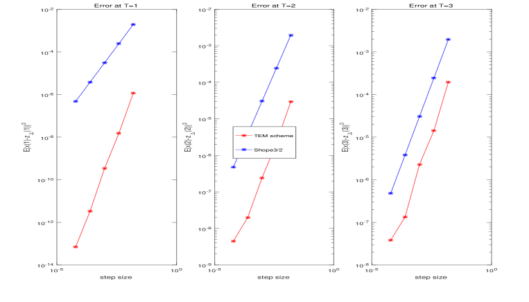
Figure 1: The red solid line depicts the $3$th moment approximation error $\mathbb{E}\left(|x(T)-z_{\triangle}(T)|^{3}\right)$ between the exact solution $x(T)$ and the TEM scheme $z_{\triangle}(T)$, as the function of $\triangle$ for 1000 sample points as $T=1,~{}2,~{}3$, and $\triangle\in\{2^{-14},~{}2^{-12},~{}2^{-10},~{}2^{-8},~{}2^{-6}\}$. The blue solid line plots the reference function $\triangle^{\frac{3}{2}}$.

Example 4.2

Consider 2-dimensional SDDE

$$\left\{\begin{array}[]{ll}\mathrm{d}x_{1}(t)=\left(-\frac{3}{2}x_{1}(t)-x_{1}^{3}(t)\right)\mathrm{d}t+x_{2}^{2}(t-1)\mathrm{d}W_{1}(t),&\\ \mathrm{d}x_{2}(t)=\left(-x_{2}(t)-x_{2}^{3}(t)\right)\mathrm{d}t+x_{1}^{2}(t-1)\mathrm{d}W_{2}(t),~{}~{}t>0,\end{array}\right.$$ (4.3)

with the initial data $(\xi_{1}(\theta),\xi_{2}(\theta))^{T}=(e^{-1.3\theta},0)^{T},~{}\theta\in[-1,~{}0]$. We compute that for any $x,~{}y,~{}\bar{x},~{}\bar{y}\in\mathbb{R}^{2}$

$$|f(x,y)-f(\textbf{0},y)|\leq\frac{3}{2}(1+|x|^{2})|x|,~{}~{}~{}|g(x,y)-g(\textbf{0},y)|^{2}\leq 2|y|^{4},$$

$$f(\textbf{0},y)=0,~{}~{}~{}|g(\textbf{0},y)|^{2}\leq 2|y|^{4},$$

and

$$\langle 2x,f(x,y)\rangle+|g(x,y)|^{2}$$

$$\leq -2|x|^{2}-2(|x_{1}|^{4}+|x_{2}|^{4})+(|y_{1}|^{4}+|y_{2}|^{4}).$$

Then (H1), (H7) and (H8) hold with $V_{2}(x)=|x_{1}|^{4}+|x_{2}|^{4}$, where $\bar{K}_{6}=2$, $K_{6}=0.6$, $\bar{K}_{7}=2$, $K_{7}=1$. Choose $\gamma=0.69$ such that

$$1.8862\approx K_{6}e^{\gamma\tau}+\gamma<\bar{K}_{6}=2,~{}~{}~{}~{}~{}1.9937\approx K_{7}e^{\gamma\tau}<\bar{K}_{7}=2.$$

By virtue of Theorem 3.4 and Theorem 3.5, (4.3) is the exponential stable in mean square and $\mathbb{P}-1$.

By (3.62), we take $\hat{\Phi}(l)=2(1+l^{2})$, where $l\geq 1$.  By (3.63) and $\|\xi\|=e^{1.3}$, we choose $h_{\hat{\Phi},\mu}(\triangle)=2(1+e^{2.6})\triangle^{-\frac{1}{100}},~{}\forall\triangle\in(0,1]$. Let $\varepsilon=0.5\in(0,\gamma)$. we choose $\bar{\triangle}=2^{-7}$ such that for any $\triangle\in(0,\bar{\triangle}]$, (3.74) holds. It follows from Theorem 3.6 and Theorem 3.7 that for any $\triangle\in(0,~{}2^{-7}]$

$$\mathbb{E}|y_{i}^{\triangle}|^{2}\leq Ce^{-0.19t_{i}},~{}\forall~{}i\geq 0,~{}~{}~{}~{}\limsup_{i\rightarrow\infty}\frac{1}{i\triangle}\log{|y_{i}^{\triangle}|}\leq-\frac{0.19}{2},~{}\hbox{a.s}.$$

Figure 2 depicts the sample mean of the TEM scheme $y_{i}^{\triangle}$ defined in (3.67). Figure 3 depicts a sample path of the EM solution $Y_{i}^{\triangle}$ and a sample path of the TEM solution $y_{i}^{\triangle}$.

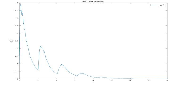
Figure 2: The sample mean of $y_{i}^{\triangle}$ with 1000 sample points, $\triangle=2^{-7}$ and $t\in[0,~{}8]$.

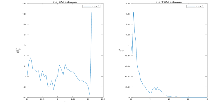
Figure 3: The sample paths of $\ln Y_{i}^{\triangle}$ by the EM and of the TEM solution $y_{i}^{\triangle}$ defined in (3.67) with $\triangle=2^{-7}$ and $t\in[0,~{}4]$.

5 Conclusions

In this paper we construct an explicit numerical scheme under the weakly local Lipschitz condition and the Khasminskii-type condition, which numerical solutions are bounded and converge to the exact solutions in $q$th moment for $q>0$. The ${1}/{2}$ order convergence rate is obtained for the TEM scheme. Moreover, in order to realize the long time dynamical behavior we propose a more precise TEM scheme. The exponential stability is kept well by the numerical solutions of the TEM for a large kind of nonlinear SDDEs.

References

- [1] Arriojas, M., Hu, Y., Mohammed, S.-E. and Pap, G., A delayed black and scholes formula, Stochastic Analysis and Applications, 25(2) (2007), 471-492.
- [2] Baker, Christopher T. and Buckwar, E., Numerical analysis of explicit one-step methods for stochastic delay differential equations, LMS Journal of Computation and Mathematics, 3 (2000), 315-335.
- [3] Bao, J., Yin, G. and Yuan, C., Asymptotic Analysis for Functional Stochastic Differential Equations, Springer, 2016.
- [4] Buckwar, E., Introduction to the numerical analysis of stochastic delay diffierential equations, Journal of Computational and Applied Mathematics, 125 (2000), 297-307.
- [5] Cong, Y., Zhan, W. and Guo, Q., The partially truncated Euler-Maruyama method for highly nonlinear stochastic delay differential equations with Markovian Switching, International Journal of Computational Methods, 17(6) (2020), 1950014.
- [6] Dareiotis, K., Kumar, C. and Sabanis, S., On tamed Euler approximations of SDEs driven by Lévy noise with applications to delay equations, SIAM Journal on Numerical Analysis, 54(3) (2016), 1840-1872.
- [7] Eurich, C. and Milton, J., Noise-induced transitions in human postural sway, Physical Review E, 54(6) (1996), 6681-6684.
- [8] Guo, Q., Mao, X. and Yue, R., The truncated Euler-Maruyama method for stochastic differential delay equations, Numerical Algorithms, 78 (2018), 599-624.
- [9] Gyöngy, I. and Sabanis, S., A note on Euler approximations for stochastic differential equations with delay, Applied Mathematics and Optimization, 68(3) (2013), 391-412.
- [10] Huang, C., Mean square stability and dissipativity of two classes of theta methods for systems of stochastic delay differential equations, Journal of Computational and Applied Mathematics, 259 (2014), 77-86.
- [11] Huang, C., Gan, S. and Wang, D., Delay-dependent stability analysis of numerical methods for stochastic delay differential equations, Journal of Computational and Applied Mathematics, 236(14) (2012), 3514-3527.
- [12] Kumar, C. and Sabanis, S., Strong convergance of Euler approximations of stochastic differential equations with delay under local Lipschitz condition, Stochastic Analysis and Applications, 32(2) (2014), 207-228.
- [13] Li, M. and Huang, C., Projected Euler-Maruyama method for stochastic delay differential equations under a global monotonicity condition, Applied Mathematics and Computation, 366 (2020), 124733.
- [14] Li, X. and Mao, X., The improved LaSalle-type theorems for stochastic differential delay equations, Stochastic Analysis and Applications, 30(4) (2012), 568-589.
- [15] Li, X., Mao, X. and Yin, G., Explicit numerical approximations for stochastic differential equations in finite and infinite horizons: truncation methods, convergence in th moment and stability, IMA Journal of Numerical Analysis, 39(4) (2019), 847-892.
- [16] Mao, X., Stochastic Differential Equations and Applications, second edition, Horwood Publishing, 2007.
- [17] Mao, X. and Rassias, M., Khasminskii-type theorems for stochastic differential delay equations, Stochastic Analysis and Applications, 23(5) (2005), 1045-1069.
- [18] Mao, X. and Sabanis, S., Numerical solutions of stochastic differential delay equations under local Lipschitz condition, Journal of Computational and Applied Mathematics, 151(1) (2003), 215-227.
- [19] Mao, X. and Yuan, C., Stochastic Differential Equations with Markovian Switching, Imperial College Press, 2006.
- [20] Niu, Y., Burrage, K. and Zhang, C., A derivative-free explicit method with order 1.0 for solving stochastic delay differential equations, Journal of Computational and Applied Mathematics, 253 (2013), 51-65.
- [21] Wang, X. and Gan, S., The improved split-step backward Euler method for stochastic differential delay equations, International Journal of Computer Mathematics, 88(11) (2011), 2359-2378.
- [22] Wu, F., Mao, X. and Kloeden, P., Discrete Razumikhin-type technique and stability of the Euler-Maruyama method to stochastic functional differential equations, Discrete and Continnous Dynamical Systems, 33(2) (2013), 885-903.
- [23] Wu, F., Mao, X. and Szpruch, L., Almost sure exponential stability of numerical solutions for stochastic delay differential equations, Numerische Mathematik, 115(4) (2010), 681-697.
- [24] Yang, H. and Li, X., Explicit approximations for nonlinear switching diffusion systems in finite and infinite horizons, Journal of Differential Equations, 265(7) (2018), 2921-2967.
- [25] Zhang, W., Yin, X., Song, M. and Liu, M., Convergence rate of the truncated Milstein method of stochastic differential delay equations, Applied Mathematics and Computation, 357 (2019), 263-281.
- [26] Zhao, J., Yi, Y. and Xu, Y., Strong convergence and stability of the split-step theta method for highly nonlinear neutral stochastic delay integro differential equation, Applied Numerical Mathematics, 157 (2020), 385-404.