Enabling Remote Whole-Body Control with 5G Edge Computing

Abstract

Real-world applications require light-weight, energy-efficient, fully autonomous robots. Yet, increasing autonomy is oftentimes synonymous with escalating computational requirements. It might thus be desirable to offload intensive computation—not only sensing and planning, but also low-level whole-body control—to remote servers in order to reduce on-board computational needs. Fifth Generation (5G) wireless cellular technology, with its low latency and high bandwidth capabilities, has the potential to unlock cloud-based high performance control of complex robots. However, state-of-the-art control algorithms for legged robots can only tolerate very low control delays, which even ultra-low latency 5G edge computing can sometimes fail to achieve. In this work, we investigate the problem of cloud-based whole-body control of legged robots over a 5G link. We propose a novel approach that consists of a standard optimization-based controller on the network edge and a local linear, approximately optimal controller that significantly reduces on-board computational needs while increasing robustness to delay and possible loss of communication. Simulation experiments on humanoid balancing and walking tasks that includes a realistic 5G communication model demonstrate significant improvement of the reliability of robot locomotion under jitter and delays likely to be experienced in 5G wireless links.

I Introduction

Legged robots are favored in many scenarios such as disaster rescue and advanced manufacturing due to their high mobility [1]. However, to cope with dynamic, ever-changing real-world environment, robots need to be vested with fast and reliable sensing, planning and control capabilities, which all require large amount of computation. However, powerful on-board computing increases the weight of the robot and its energy consumption, and consequently affects the autonomy of the robot. For example, ANYmal, one of the most advanced commercially available quadruped robot, carries $3\text{\,}\mathrm{kg}$ of batteries of about $650\text{\,}\mathrm{W}\text{\,}\mathrm{h}$ energy [2] while the high-end Nvidia Titan X consumes more than $250\text{\,}\mathrm{W}$ of power, significantly impacting battery life if such computational power was embedded on the robot.

The idea of offloading computations to the cloud is not novel [3] and has attracted a lot of attention for tasks that do not require real-time performance. Nevertheless, cloud computing remains elusive for latency-critical tasks as limited bandwidth and high latency of wireless communication preclude the transmission of rich multi-modal sensor data to the cloud and the remote execution of fast millisecond scale feedback control loops.

5G cellular network edge computing technology [4] in conjunction with massive broadband links in the millimeter wave (mmWave) bands [5, 6] offer unprecedented access to high bandwidth and low latency communication that could render edge-based real-time control a reality. In traditional wide area networks, packets are typically routed through a centralized gateway before accessing any cloud services. This routing can cause considerable delay—in excess of $40\text{\,}\mathrm{ms}$ in current 4G LTE networks [7]. 5G edge computing, i.e. when the computers are placed at the edge of the network, close to the wireless base stations, dramatically reduces the delay in the core network. At the same time, the mmWave bands offer vast amounts of spectrum that enable ultra-fast communication in the airlink enabling delays of $12\text{\,}\mathrm{ms}$, an order of magnitude lower delays than current 4G links operating in traditional spectrum bands, and within the requirements of state of the art torque control methods [8].

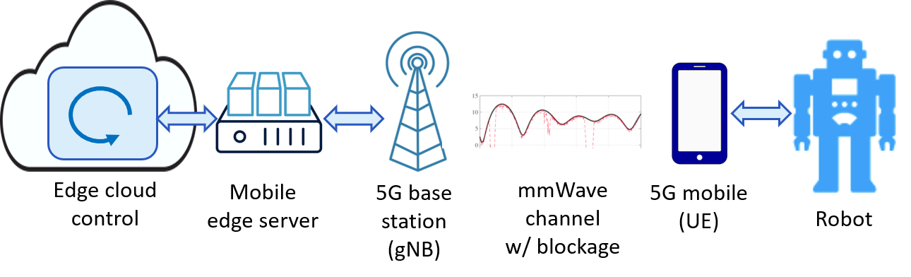
Figure 1: Cloud-based robotic edge whole-body control over a 5G mmWave wireless link.

However, a key challenge with communication in the mmWave bands is that the signals are highly susceptible to blockage by common materials in the environment including buildings, people, and foliage [9, 10, 11, 12]. Robots with metallic parts can also block mmWave signals. As a result, links can intermittently experience outage causing delays, jitter and packet loss. These outages are not permanent as signals can be re-routed or communication can fallback to the 4G network but nevertheless create significant delays. Although robots may be able to detect such circumstances and adapt their behavior accordingly using models of mmWave signal propagation [13], such adaptation of the plan inevitably introduces a nonnegligible time window during which the robot needs to operate under increased communication delays or absence of communication with the network edge.

State-of-the-art whole-body controllers for legged robots are computationally expensive as they typically require the resolution of quadratic programs at a control frequency of $5001000\text{\,}\mathrm{Hz}$ [14]. For example, in [8], one core of a CPU was entirely dedicated to the computation of the control commands. While local computational requirements would significantly decrease by offloading whole-body control to the edge, communication loss or delays are an important challenge as these feedback controllers are very susceptible to delays to maintain proper operating conditions and resist unexpected disturbances. This is especially important for legged robots that need to walk in uncertain environments.

In this work, we propose and study the first edge-based whole-body controller over a 5G communication link capable of handling communication loss and delays as depicted in Fig. 1. Our approach provides an efficient local control algorithm to enhance the performance of a purely remote controller in face of delays. The algorithm separates the computationally expensive part of the control problem and approximates it with a linear feedback controller based on previously obtained information from the external, full capacity controller. Together with the local information measured by the robot, it creates an approximately optimal control command to reduce the violation of task constraints and thus achieve the tasks in the presence of delays. We present a complete simulation environment including a realistic 5G communication model and rigid-body dynamics. Extensive simulations demonstrate the capabilities of the approach for bipedal balancing and walking tasks in disaster response and manufacturing environments.

II Background

II-A Task-space inverse dynamics

In recent years, optimization-based task-space inverse dynamics [15, 16, 17, 18] has become ubiquitous for the control of legged robots as it provides a simple yet principled way of formulating task-space inverse dynamics problems as Quadratic Programs; and more importantly, allows more flexible task descriptions using inequality constraints (e.g. to impose actuation limits or friction cone constraints).

Denoting the robot configuration as $q\in SE(3)\times\mathbb{R}^{j}$, the joint torque as $\tau\in\mathbb{R}^{j}$, where $j$ is the number of the joints, the dynamics of a robot in rigid contact can be written as

$$M\ddot{q}+h =S^{\mathsf{T}}\tau+J^{\mathsf{T}}_{c}f$$ (1a)

$$J_{c}\ddot{q}+\dot{J}_{c}\dot{q} =0\,,$$ (1b)

where $M$ is the generalized inertia matrix; $h$ is a vector of generalized forces including gravity, centrifugal and Coriolis forces; $S^{\mathsf{T}}$ maps actuated joints torques to the generalized coordinates; $f$ denotes the contact forces, and $J_{c}$ is the Jacobian of the contact points.

A task function $s(q)$ maps the robot configuration to the task space, and a desired closed-loop task-space controller is given by $\ddot{s}^{*}$. For example, $s(t)$ can be the Center of Mass (CoM) position; and $\ddot{s}^{*}$ would be the desired CoM acceleration computed from a desired closed-loop CoM dynamics. Task-space inverse dynamics aims to find $\ddot{q},\tau,f$ that satisfy physical consistency constraints while achieving several tasks as well as possible, i.e. getting $\ddot{s}-\ddot{s}^{*}$ as small as possible in the least-square sense. Note that $\tau$ is uniquely determined by $\ddot{q},f$ from (1a) and that the dynamic consistency equation can be reduced to a 6D equation [17] by considering only the unactuated part of the dynamics. The problem can therefore be formulated as a QP solving for the stacked variable $y=(\ddot{q},f)\in\mathbb{R}^{n}$

$$\underset{y=(\ddot{q},f)}{\text{minimize}} \frac{1}{2}\sum_{i}\omega_{i}\left\lVert J_{i}\ddot{q}+\dot{J}_{i}\dot{q}-\ddot{s}_{i}^{*}\right\rVert^{2}$$ (2a)

subject to $$Ay\leq b\,,$$ (2b)

where $\omega_{i}>0$ weights the relative importance of each task and $J_{i}=\frac{\partial s_{i}}{\partial q}$ is the Jacobian of task $i$ that satisfies $\dot{s}_{i}=J_{i}\dot{q}$. Eq. (2b) summarizes all equality and inequality constraints by stacking $K$ constraints $a_{k}^{\mathsf{T}}y\leq b_{k},\ \forall k=0,1,\dots,K$ into the matrix $A$ and the vector $b$, including the dynamic and contact constraints equations (1). Note that in this section we only describe kinematic tasks depending on $\ddot{q}$ for simplicity but force tasks depending on $f$ can be similarly formulated and all results presented in the following trivially carry over to this case.

II-B Active-set method

We solve the constrained QP (2) using an active-set method. Given $y$, a constraint $a_{k}^{\mathsf{T}}y\leq b_{k}$ is called active when $a_{k}^{\mathsf{T}}y=b_{k}$. The active set $\mathcal{A}$ contains thus all equality constraints and the inequality constraints that are satisfied with equality, i.e. $a_{k}^{\mathsf{T}}y=b_{k},\ \forall k\in\mathcal{A}$. Starting from an initial guess of the active-set, an equality constrained problem

$$\underset{y=(\ddot{q},f)}{\text{minimize}} \frac{1}{2}\sum_{i}\omega_{i}\left\lVert J_{i}\ddot{q}+\dot{J}_{i}\dot{q}-\ddot{s}_{i}^{*}\right\rVert^{2}$$ (3a)

subject to $$\bar{A}y=\bar{b}\,,$$ (3b)

is solved at each iteration of the active-set search. $\bar{A}$ and $\bar{b}$ represent the constraints in the current iterate of the active set. If at the current solution ${y}^{*}$ to  (3), there are inequality constraints being violated, one of them will be added (activated) to the active set. Otherwise, an inequality constraint that prevents the solution from going closer to the optimum will be removed (deactivated). The algorithm converges if no inactive violated constraints remain and no active constraints need to be deactivated. At this point the optimal active-set $\mathcal{A}_{\text{opt}}$ is found, and we denote by $\bar{A}_{\text{opt}},\bar{b}_{\text{opt}}$ the stacked matrix and vector of the constraints $a_{k}^{\mathsf{T}}y=b_{k},\ \forall k\in\mathcal{A}_{\text{opt}}$.

The solution ${y}^{*}$ to (3) is found by the Nullspace method [19]. A structured formulation is given by the publicly available solver in [14]: here the solution

$$y^{*}=\underline{A}^{\ddagger}\underline{b}$$ (4)

is found with the hierarchical inverse $\underline{A}^{\ddagger}$. $\underline{A}$ and $\underline{b}$ denote the stacked matrix and the stacked vector

$$\underline{A} =\begin{bmatrix}\bar{A}^{\mathsf{T}}&w_{1}J_{1}^{\mathsf{T}}&\dots&\end{bmatrix}^{\mathsf{T}}$$ (5)

$$\underline{b} =\begin{bmatrix}\bar{b}^{\mathsf{T}}&w_{1}(-\dot{J}_{1}\dot{q}+\ddot{s}_{1}^{*})^{\mathsf{T}}&\dots&\end{bmatrix}^{\mathsf{T}}\,,$$ (6)

respectively. Note that $\underline{A}^{\ddagger}$ is only given implicitly when computing $y^{*}$ by a forward recursion using the Hierarchical Complete Orthogonal Decomposition (HCOD) of $\underline{A}$. This is implied throughout the paper when using the expression $\underline{A}^{\ddagger}$. The computation of the HCOD requires $O(2n^{3})$ operations, while the complexity of the forward recursion is $O(n^{2})$ with $n$ being the number of decision variables. This scheme is potentially applicable to hierarchical problems with any number of priority levels.

In the following, $\underline{A}^{\ddagger}_{\text{opt}}$ is associated to the HCOD of the optimal active set $\bar{A}_{\text{opt}},\bar{b}_{\text{opt}}$ found for (3).

II-C 5G Cloud Edge Computing

Our goal is to study robotic control in scenarios where some of the computation is offloaded to an edge server over a 5G mmWave wireless link. The basic model is shown in Fig. 1. The robot is equipped with a wireless 5G mobile device, called the User Equipment (UE), which is functionally similar to a smartphone. The UE communicates wirelessly to a base station over a mmWave channel. In 5G terminology, the base station is called the gNB [20, 21]. The mmWave bands are a key component of the 5G standard which use high bandwidth signals transmitted in narrow electronically steerable beams. These signals offer massive peak rates ($>$1\text{\,}\mathrm{G}\mathrm{bit}\mathrm{/}\mathrm{s}$$) with very low latency ($12\text{\,}\mathrm{ms}$) over the airlink.

The latency over the airlink (the wireless connection between the UE and gNB) is not the only component of delay. In a traditional 4G cellular network, data must be typically routed to centralized gateway before it can access any third-party cloud services [22, 23]. This architecture can add considerable delay—often in excess of $40\text{\,}\mathrm{ms}$ [7]. To enable low end-to-end delay, 5G networks can combine a low latency airlink with mobile edge cloud architecture [4]. As shown in Fig. 1, data from the base stations can be routed to a mobile edge server that can host edge cloud services that have much lower delay to the base stations—potentially as low as a few milliseconds, depending on the deployment. As per the latest 5G system architecture [24] defined by 3GPP the 5G Core Network selects a User Plane Function (UPF) close to the UE and executes the traffic steering from the UPF to the local Data Network via a N6 interface.

The basic problem we consider in this work is how to partition the control between the local computation on the robot and remote computations on the edge server. The key challenge is that, while 5G mmWave links offer very high peak rates, the signals are intermittent due to blockage as discussed in the introduction [9, 10, 11, 12]. Thus, we wish to find distributed control policies that can exploit low-latency cloud resources when the wireless links are available, but are robust during blockage and outage events.

III Locally assisted remote whole-body control

III-A Structure of the QP solution

The QP solution (4) has several interesting properties: First, the matrix $\underline{A}^{\ddagger}_{\text{opt}}$ depends only on the task Jacobians $J_{i}$ and the optimal active set normal $\bar{A}_{\text{opt}}$. The matrix $\bar{A}_{\text{opt}}$ will change as a function of $q$ and $\dot{q}$, but this change—similarly to the Jacobians—will be rather slow. Thus, the matrix $\underline{A}^{\ddagger}_{\text{opt}}$ will not change too much in a short period of time as long as the optimal active set $\mathcal{A}_{\text{opt}}$ remains the same. This implies that a delayed $\underline{A}^{\ddagger}_{\text{opt}}$ will still approximately enforce all the active constraints if $\underline{b}_{\text{opt}}$ is updated sufficiently fast. Fortunately, $\underline{b}_{\text{opt}}$ only depends on the generalized forces $h$, the robot state $q,\dot{q}$, the task reference $\ddot{s}^{*}$, the task Jacobian $J_{i}$, and its time derivative $\dot{J}_{i}$. These quantities can all be stored and updated efficiently without querying a remote server, as forward kinematics and Jacobian computations can be done in $O(n)$, where $n$ is the robot’s number of Degrees of Freedom. Constructing $\underline{b}_{\text{opt}}$ from these quantities also only requires basic matrix operations that a low-power on-board computer can easily execute. Notably, all the error feedback terms are contained in $\underline{b}_{\text{opt}}$ which therefore renders it the most important quantity for control, while the matrix $\underline{A}^{\ddagger}_{\text{opt}}$ can be seen as a projector that changes slowly.

These properties naturally partition the optimal control command into two parts:

1. the computation of $\underline{A}^{\ddagger}_{\text{opt}}$ which is expensive but less susceptible to delays; and

2. the construction of $\underline{b}_{\text{opt}}$ which contains the error feedback terms and is latency-critical but can be done efficiently.

In this paper, we propose to offload the active-set search and the computation of $\underline{A}^{\ddagger}_{\text{opt}}$ to the remote server, while updating $\underline{b}_{\text{opt}}$ locally on the robot. If the robot fails to recover the latest decomposition $\underline{A}^{\ddagger}_{\text{opt}}$ due to communication delays or packet loss, we approximate it with the most recently received one. This still enables us to perform feedback control for all the tasks and to approximately enforce previously active inequality constraints.

III-B Control scheme

These insights together give rise to the following control scheme illustrated in Fig. 2. At any time $t$, the robot maintains a cache of the decomposition $\underline{\hat{A}}^{\ddagger}_{\text{opt}}$ and the optimal active set $\mathcal{\hat{A}}_{\text{opt}}$ from the most recently successful communication with the remote server, and the robot measures its state $q,\dot{q}$ and constructs the vector $\underline{b}_{\text{opt}}$; then it sends $q,\dot{q}$ to the remote controller to solve the full QP problem (2). Meanwhile, the robot computes the approximate command

$$\hat{y}=\underline{\hat{A}}^{\ddagger}_{\text{opt}}\underline{b}_{\text{opt}}\,.$$

Note that the active-set search is not continued according to the changed right hand side $\underline{b}_{\text{opt}}$ as it is potentially expensive if a lot of active-set iterations are necessary. Instead, the last found optimal active-set $\mathcal{\hat{A}}_{\text{opt}}$ is used when computing the approximate solution.

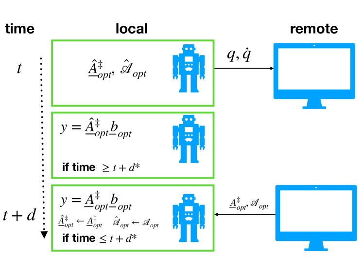
Figure 2: Communication and computation flow between the robot and the edge computer in the proposed control scheme.

At time $t+d$, the robot receives a new decomposition $\underline{{A}}^{\ddagger}_{\text{opt}}$ and the new optimal active set $\mathcal{A}_{\text{opt}}$ from the remote controller, where the delay $d$ depends on the communication channel. The local cache is updated accordingly. Note that this solution may not have been computed based on the state $q,\dot{q}$ measured at time $t$ due to the previous delays.

Given the period of the control loop $T$ (e.g. $T=$1\text{\,}\mathrm{ms}$$), we can set a desired threshold $0<d^{*}<T$ such that the robot applies a control command

$$y=\begin{cases}\underline{A}^{\ddagger}_{\text{opt}}\underline{b}_{\text{opt}}&\text{ if }d<d^{*}\\ \hat{y}&\text{ otherwise }\,.\end{cases}$$ (7)

At time $t+T$, the process described above repeats.

III-C Handling contact switches

The control scheme described above relies on the assumption that the optimal active set does not change when the communication delay occurs. This assumption is plausible for tasks where no contact is broken or established when blocking events occur, such as balancing without external disturbances. However, for contact-switching tasks such as walking, this assumption becomes problematic for two reasons 1. the contact switches introduce very different constraints and thus different optimal active sets; and 2. even in the same contact mode, when the robot approaches the contact switch, the optimal active set changes more frequently due to the friction cone constraints being activated.

To resolve the first issue, we pre-compute the solution to the new contact mode shortly before the contact switch by imposing the new contact constraints on the current robot state. This gives a valid approximation for low-speed locomotion because the state of the robot $q,\dot{q}$ shortly before and after the contact switch is similar. The solution differs mostly due to the different contact forces and the corresponding constraints. Therefore, if the contact switch does happen and we have not yet obtained the corresponding optimal solution from the remote server, we can use the pre-computed solution and approximately enforce the new constraints. On the other hand, for highly dynamic locomotion, the generalized velocity $\dot{q}$ may change significantly across contact switches; to tackle this issue, a more sophisticated prediction of the state $q,\dot{q}$ is required, which we leave for future work.

While this pre-computation can in principle be performed on the edge computer, it has to be completed before the contact switch occurs. However, it is difficult to have a delay upper bound in the 5G network and this upper bound might anyway be too large compared to the timing of one step. In this case, we additionally use the on-board computer to perform the pre-computation. As we assume that the on-board computer has very limited computational capabilities, the QP needs to be started several control cycles prior to the switch. The delay introduced by the on-board computation can be considered upper-bounded by a constant in practice as will be shown in the simulation experiments.

The second issue can also be mitigated in a similar manner—we can solve the full QP problem (2) on-board as well when the contact switch is happening, as the optimal active set is more likely to be similar in a shorter period.

In our implementation, in the time window of length $100\text{\,}\mathrm{ms}$ centered at the planned contact switch time, we perform all computation—including the full QP, the local controller, and the pre-computation (once per contact switch) of the next contact mode—locally, i.e. on the on-board computer. Note, in this case we choose to solve the full QP every $5\text{\,}\mathrm{ms}$ due to limited computational capacity. In addition, the pre-computation will be initiated $10\text{\,}\mathrm{ms}$ before the planned contact switch time. The aforementioned choice of numbers is reasonable for our simulated low-power on-board computer, as later simulation experiments will show that it takes less than $3\text{\,}\mathrm{ms}$ to solve the full QP locally in the worst case. We do still query the remote server to solve the full QP at the same time, so that we get better approximation when the communication with the server is faster than the on-board computation. The increase in on-board computational complexity is minimal as full QPs are only solved on-board in a short period of time around contact switches at a much lower speed than the control frequency.

It is worth noting that the way we handle contact switches as described above heavily relies on the accurate knowledge of when and how the contact switch will happen, resulting in lack of robustness of our approach to unexpected contacts. However, a principled handling of unexpected contact switches is still an open problem for optimization-based task-space inverse dynamics controllers even without control delays. Addressing this issue therefore goes beyond the scope of this paper and we leave the question of robustness to unexpected contact changes to future research.

IV Simulation experiments

In the following simulation experiments, we compare our locally assisted remote control scheme (LA) with a purely remote control scheme (PR). PR sends the measured robot state to the remote controller to compute the optimal solution. If the robot does not recover the latest command from the remote controller, executes the most recently received command. The goal of these experiments is to demonstrate that our approach significantly improves robustness to delays with limited computational overhead.

The simulation experiments consist of robot balancing and walking tasks under two different delay settings: constant delays and simulated stochastic delays in 5G networks. The simulations were conducted on an Intel Xeon CPU at $3.7\text{\,}\mathrm{GHz}$. The on-board computer of the robot is emulated by restricting the computation to a single core of the CPU at $1.2\text{\,}\mathrm{GHz}$. We simulate the $37$-DoF humanoid robot Romeo and use Pinocchio [25] for rigid body dynamics computation.

IV-A Robot tasks

Our control scheme is evaluated on two typical tasks for legged robots, namely balancing and walking.

1. Balancing The task is achieved by stabilizing the CoM of the robot while maintaining rigid contacts between the feet and the ground. To prevent slipping, we constrain the ground reaction forces to stay inside the friction cones approximated with $4$-sided pyramids. In addition, we minimize an error between the current joint positions and a desired upright posture in the whole-body joint space to resolve remaining torque redundancies. We inject Gaussian noise with a noise level $\sigma=1\times 10^{-2}$ to the joint measurements and apply an external push of $100\text{\,}\mathrm{N}$ for $0.2\text{\,}\mathrm{s}$ at the robot base.

2. Walking For this task, we first generate offline a desired CoM trajectory and a footstep plan using a linear inverted pendulum model [26]. The motion of the swing foot is synthesized by interpolating splines from one step location to another and each step takes $0.8\text{\,}\mathrm{s}$. The robot alternates between single support phase (one foot on the ground) and short double support phases of $5\text{\,}\mathrm{ms}$ (both feet on the ground) by following the desired CoM trajectory and foot motion. In the double support phase, both feet have to obey rigid contact constraints and friction cone constraints, while in the single support phase, only the support foot needs to respect those two constraints. The measurement noise level is $\sigma=1\times 10^{-3}$ in this task.

The task objectives and constraints are formulated by TSID [27] and then solved as a constrained QP by the solver [14] as described in Sec. II-B.

IV-B Network and wireless modeling

The communication between the server and the robot over the 5G channel is simulated using ns-3 [28], a widely-used open-source network simulator. We use a state-of-the-art 5G mmWave module in ns-3 to simulate the wireless link and network stack [29] used in several works [30, 31]. This module includes detailed models for the wireless channel, wireless communication stack, core network and networking protocols. We use MmWave3GPPPropogationLossModel to configure the communication channel. Note that at the time of writing, real 5G base stations were not available.

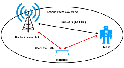
(a) No blockage

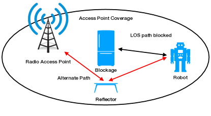
(b) With blockage

Figure 3: Illustration of Line of Sight and Multipath of the signal for non-blocking and blocking scenarios respectively

Our key task is to analyze the robustness due to blockage. To model this, we follow [31, 30] where several moving obstacles are placed in the environment and blockage is computed via ray tracing. We assume fixed number of blockers in the environment and fully digital beamforming to expedite beam search during blocking events.

Fig. 3b illustrates the blocking scenario in the simulation. The blockages move at a speed of $2\text{\,}\mathrm{m}\mathrm{/}\mathrm{s}$. Table I details the parameters used in the ns-3 simulation. The type of blockages and the distance between the access point and the robot is dependent on the simulation scenarios. We consider two scenarios relevant for legged robot applications (parameters for both scenarios can be found in [29]):

1. Smart factory This scenario models the case where robots conduct manufacturing tasks autonomously or with humans. The access point is placed in the middle of the factory; the robot or the blockages can move around it. Solid metal and stone blockages are used in this scenario. It is characterized by infrequent blocking events as the factory environment is well structured. However, delays introduced by blocking events can be as high as $389\text{\,}\mathrm{ms}$ as potential blockages such as containers and manufacturing components are large in size.

2. Burning building This is a mission critical scenario, where a robot is sent inside a burning building to analyze and report back possible threats. The access point is placed on a window while the robot is mobile inside. The blockages in this case are in close proximity of each other and are smaller in size. The type of blockages used are wooden or solid metal. This results in a delay profile characterized by frequent but lower delays; the maximal delay in this scenario does not exceed $91\text{\,}\mathrm{ms}$.

We also note that the simulated delays do not reflect the possible damage to the access point in the burning building scenario.

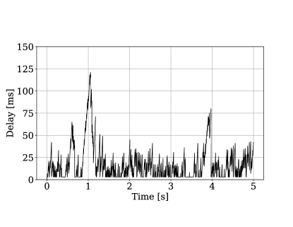
(a) Smart factory

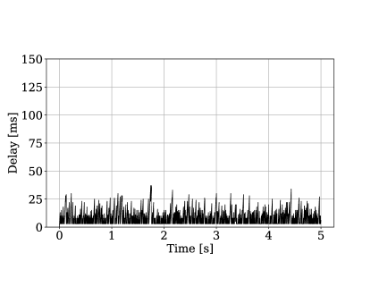
(b) Burning building

Figure 4: An instance of the delay profile in each of the simulated scenarios.

TABLE I: ns-3 simulation parameters

Parameters	Smart factory	Burning building
Channel model	UMi-StreetCanyon	InH-OfficeMixed
Maximal distance between	$100\text{\,}\mathrm{m}$	$30\text{\,}\mathrm{m}$
the access point and robot
Bandwidth	$1\text{\,}\mathrm{GHz}$
Number of blockers	4
Transport layer protocol	UDP
Maximal uplink packet size	$1\text{\,}\mathrm{kB}$
Maximal downlink packet size	$40\text{\,}\mathrm{kB}$
Transmission frequency	$1\text{\,}\mathrm{kHz}$

In both scenarios above, we have assumed a delay from the base station to the mobile edge server of $1\text{\,}\mathrm{ms}$, a realistic value for future 5G edge deployments. At the transport layer, we have assumed UDP instead of TCP. TCP ensures packet delivery using re-transmissions whereas UDP transmits only once and does not wait for any acknowledgement or ensure packet delivery. Since our robotics automation loop discards any packet that does not meet the specified time constraints, re-transmission would only lead to excessive bandwidth consumption and cause more delay.

Fig. 4 shows an instance of the delay profile in each of the scenarios under these assumptions. We generated $100$ different delay profiles for each scenario by randomizing the initial positions of the robot and the blockages. The delay profiles are then introduced into the robotics simulator to assess the effect of the delay.

IV-C Metrics

We examine the control performance by measuring the average CoM tracking error and the average violation of the rigid contact constraint

$$\frac{1}{N}\sum_{n=0}^{N}\left\lVert p-p_{d}\right\rVert\,\text{ and }\frac{1}{N}\sum_{n=0}^{N}\left\lVert J_{c}\ddot{q}+\dot{J}_{c}\dot{q}\right\rVert\,,$$

where $N$ is the total number of the simulation steps; $p$ and $p_{d}$ denotes the actual and desired CoM position; the time indices are dropped for notational simplicity. Due to symmetry, we only report the constraint violation of the left foot for the balancing task; for the walking task, we report the constraint violation of the support foot.

Finally, whether a robot falls or not is used as a qualitative metric to determine the failure or success of a task execution.

IV-D Results

Constant delays

Table II and Table III report the performance of PR and LA in the balancing task and the walking task respectively. The infinity symbol $\infty$ in the tables indicates that the robot fell. The last row of the tables shows the maximal tolerable delay for LA to achieve the task without the robot falling. Recall that we require on-board computation for the walking task—here we simply assume that the on-board computation causes the same respective constant delays; for instance, a $25\text{\,}\mathrm{ms}$ constant delay means that we solve the full QPs onboard every $25\text{\,}\mathrm{ms}$. Different constant delays can be interpreted as the usage of different on-board computational capacities. Across all delay levels, LA had lower tracking error and lower constraint violation than PR. The maximal tolerable constant delay was significantly increased by incorporating the local controller in both the balancing task and the walking task. An important implication of this result is that our approach can also be used to address the delay caused by limited on-board computational resources if the on-board computation scheme is properly scheduled to produce bounded delays, enabling purely local optimization-based whole-body control on a low-power on-board computer. It is thus interesting for future research to investigate the control performance and power consumption of such schemes compared to our locally assisted remote control scheme.

TABLE II: Balancing task performance of PR and LA under various constant delays. The last row shows the maximal delay LA can tolerate.

Delays	CoM error [$\text{\,}\mathrm{cm}$]		Constraint violation [$\text{\,}\mathrm{m}\mathrm{/}\mathrm{s}^{2}$]
	PR	LA	PR	LA
$0\text{\,}\mathrm{ms}$	1.30	1.30	0.00	0.00
$10\text{\,}\mathrm{ms}$	1.35	1.34	2.18	0.04
$20\text{\,}\mathrm{ms}$	1.43	1.38	2.17	0.04
$30\text{\,}\mathrm{ms}$	1.63	1.46	2.21	0.05
$40\text{\,}\mathrm{ms}$	2.21	1.57	2.40	0.05
$50\text{\,}\mathrm{ms}$	$\infty$	1.73	$\infty$	0.06
$90\text{\,}\mathrm{ms}$	$\infty$	2.53	$\infty$	0.16

TABLE III: Walking task performance of PR and LA under various constant delays. The last row shows the maximal delay LA can tolerate.

Delays	CoM error [$\text{\,}\mathrm{cm}$]		Constraint violation [$\text{\,}\mathrm{m}\mathrm{/}\mathrm{s}^{2}$]
	PR	LA	PR	LA
$0\text{\,}\mathrm{ms}$	1.68	1.68	0.00	0.00
$3\text{\,}\mathrm{ms}$	4.52	1.68	5.21	0.02
$5\text{\,}\mathrm{ms}$	$\infty$	1.71	$\infty$	0.03
$25\text{\,}\mathrm{ms}$	$\infty$	1.89	$\infty$	0.41

Simulated delays with blockage

As described in Sec. IV-B, we simulated two different scenarios and generated $100$ delay profiles for each scenario. For the balancing task, both the naive remote controller PR and LA managed to keep the robot in balance with high success rate. However, even though PR was able to complete the task, LA was still advantageous in the sense that it reduced the CoM tracking error and the constraint violation. As shown in Fig. 5, the constraint violation was significantly reduced except when the robot was being pushed.

For the walking task, we simulated on-board full QP computation as described in Sec. III-C by restricting the computation on a single core of the CPU at $1.2\text{\,}\mathrm{GHz}$ within a time window of length $100\text{\,}\mathrm{ms}$ centered at the planned contact switch time. In addition, the pre-computation for contact switch was initiated $10\text{\,}\mathrm{ms}$ before the contact switch. While real hardware implementation will be required to obtain a better estimate of the delay upper bound, $10\text{\,}\mathrm{ms}$ is a reasonable value as we will show later that the full QP for the tasks can be solved in less than $3\text{\,}\mathrm{ms}$ on a single core of the CPU at $1.2\text{\,}\mathrm{GHz}$. The experiments have shown that the naive approach PR could not prevent the robot from falling on the ground in either of the scenarios, while LA completed the walking task with a lower success rate in the smart factory scenario. This suggests that higher delay peaks, even with less frequent occurrence, is more damaging to the control performance than frequent delay peaks of smaller magnitude. This is particularly relevant when there is a large change in the optimal active set, for example when changing contacts.

Fig. 6 illustrates the control performance of LA in one instance of the smart factory scenario. It can be seen that there is a correlation between higher delays and larger constraint violation; especially around $0.5\text{\,}\mathrm{s}$ and $4.2\text{\,}\mathrm{s}$ the two delay peaks have caused very large constraint violation. On the other hand, while the pre-computation of the contact switch caused large discrepancy between the cached and the true optimal active set, the control performance was not significantly deteriorated due to the effective lower delay permitted by the on-board computation of full QPs.

TABLE IV: Task performance of PR and LA in the two scenarios. Performance metrics are computed from only successful trials.

Scenario	Metrics	PR		LA
		Balance	Walk	Balance	Walk
Factory	Success rate	98$\%$	$0\%$	$\mathbf{99\%}$	$\mathbf{85\%}$
	CoM error [$\text{\,}\mathrm{cm}$]	2.60	-	1.46	2.19
	Constraint violation [$\text{\,}\mathrm{m}\mathrm{/}\mathrm{s}^{2}$]	0.77	-	0.03	0.84
Building	Success rate	$\mathbf{100\%}$	$0\%$	$\mathbf{100\%}$	$\mathbf{100\%}$
	CoM error [$\text{\,}\mathrm{cm}$]	1.39	-	1.37	1.83
	Constraint violation [$\text{\,}\mathrm{m}\mathrm{/}\mathrm{s}^{2}$]	0.40	-	0.03	0.05

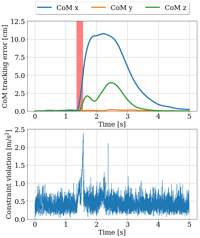
(a) PR control scheme

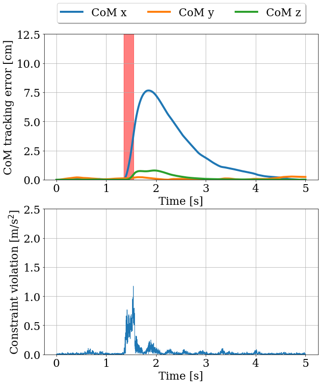
(b) LA control scheme

Figure 5: Typical control performance of PR and LA for the balancing task in the smart factory scenario. Red shaded area indicates the time window where we apply a push.

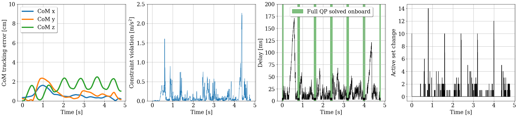
Figure 6: Typical delay profile and control performance of LA (walking in the smart factory scenario). Measurement noise is removed in the plot to better illustrate the relationship between delays and performance metrics.

TABLE V: Computation time in milliseconds of the local controller and the full QP for the walking task on a single core of the CPU at $1.2\text{\,}\mathrm{GHz}$ and $3.7\text{\,}\mathrm{GHz}$ respectively.

CPU frequency	Average		Worst
	QP	Local	QP	Local
$3.7\text{\,}\mathrm{GHz}$	0.36	0.09	0.70	0.22
$1.2\text{\,}\mathrm{GHz}$	1.21	0.30	2.39	0.76

Robustness to active set discrepancy

Our approach assumes that the optimal active set does not change during network delays or communication loss. However, it is inevitable that the cached active set may differ from the true one when the delays are too high and the active set rapidly changes, for example, when the robot switches contact or receives an unexpected push. While we have shown that our approach enabled the robot to complete the task under such circumstances, we further demonstrate empirically how the discrepancy between the cached optimal active set and the true one, hence the cardinality $|(\mathcal{A}_{\text{opt}}\cup\mathcal{\hat{A}}_{\text{opt}})\backslash(\mathcal{A}_{\text{opt}}\cap\mathcal{\hat{A}}_{\text{opt}})|$, affects the control performance in Table VI. Recall that all the equality constraints belong to the active set and the only inequality constraints we imposed are friction cone constraints, hence the change in the optimal active set is always caused by the contact force reaching the friction cone limit. For the walking task, the increased number of different constraints in the active set neither suggests higher CoM tracking error nor higher constraint violation. Indeed, the control performance deteriorates the most when there are about 5 different active constraints. For the balancing task on the other hand, the control performance worsens as long as there is any different active constraints—here we note that the source of the discrepancy in the optimal active set is different for the two tasks considered: for the balancing task, the cached optimal active set differs from the true one when the external push was applied; in the walking task, discrepancy occurs when the robot approaches contact switch, most notably when the pre-computed solution for the next contact mode was used.

TABLE VI: Performance of LA in the burning building scenario when the cached optimal active set differs from the true one. The cardinality of active set discrepancy is defined as $|(\mathcal{A}_{\text{opt}}\cup\mathcal{\hat{A}}_{\text{opt}})\backslash(\mathcal{A}_{\text{opt}}\cap\mathcal{\hat{A}}_{\text{opt}})|.$

Cardinality of	CoM error [$\text{\,}\mathrm{cm}$]		Constraint violation [$\text{\,}\mathrm{m}\mathrm{/}\mathrm{s}^{2}$]
active set discrepancy	Walk	Balance	Walk	Balance
0	1.78	0.01	0.05	0.02
1	1.91	0.05	0.06	0.19
2	1.88	0.05	0.06	0.15
3	1.90	0.06	0.08	0.13
4	2.06	0.06	0.10	0.12
5	2.06	0.06	0.19	0.14
6	1.92	0.06	0.24	0.12
7	1.54	0.06	0.09	0.12
8	1.45	0.06	0.08	0.12
9	1.38	0.06	0.06	0.11
10	1.44	0.06	0.17	0.10
11	1.40	0.06	0.18	0.10
12	1.47	-	0.19	-
13	1.52	-	0.18	-
14	1.41	-	0.19	-

Computation time

We report in Table V the average and worst-case computation time of 1. solving the full QP (2); and 2. constructing the local controller (4) for the walking task in the burning building scenario. The computation time was obtained when the computation was restricted on a single core of the CPU at $1.2\text{\,}\mathrm{GHz}$ and $3.7\text{\,}\mathrm{GHz}$ respectively to emulate a low-power on-board computer required by LA and a high-performance computer by traditional purely local optimization-based whole body inverse dynamics controller. It can be seen that the local controller computation takes significantly less time than solving a full QP. This is not surprising, as the time complexity of the QP is dominated by the HCOD of cubic complexity $O(2n^{3})$ where $n$ is the number of decision variables; in our case, $n=61$. In the case of changes in the active-set, the decomposition is updated in approximately $O(2n^{2})$ operations. On the other hand, the local controller computation is only dominated by a matrix-vector multiplication of time complexity $O(n^{2})$ and can be parallelized if needed.

V Conclusion

In this work, we have presented the first edge-based whole-body control algorithm over a 5G wireless link subject to unpredictable realistic delays. The proposed algorithm complements the remote controller on the network edge to robustly complete the task when there is a temporary unexpected communication delay. Simulation results have shown that the algorithm significantly improves control performance for balancing and walking tasks under both constant and stochastic delays. The proposed local controller is much more efficient than solving a full QP, such that it can be executed on a low-power on-board computer with limited computational resources. We do emphasize that our current framework requires solving full QPs onboard when switching contacts. Although this is a benign requirement, it would be an interesting future research direction to explore the possibilities of handling contact switches when delay occurs, without solving the full QP locally. For example, we can monitor and predict the channel quality online and only make contact switch when we are confident in the connectivity. Another option would be computing offline the QP solution in an explicit MPC manner so that it can be stored locally on the robot and be inquired when needed.

References

- [1] A. Kheddar, S. Caron, P. Gergondet, A. Comport, A. Tanguy, C. Ott, B. Henze, G. Mesesan, J. Englsberger, M. A. Roa, P. Wieber, F. Chaumette, F. Spindler, G. Oriolo, L. Lanari, A. Escande, K. Chappellet, F. Kanehiro, and P. Rabaté, “Humanoid robots in aircraft manufacturing: The airbus use cases,” IEEE Robotics Automation Magazine, vol. 26, no. 4, pp. 30–45, 2019.
- [2] M. Hutter, C. Gehring, D. Jud, A. Lauber, C. D. Bellicoso, V. Tsounis, J. Hwangbo, K. Bodie, P. Fankhauser, M. Bloesch, R. Diethelm, S. Bachmann, A. Melzer, and M. Hoepflinger, “ANYmal - a highly mobile and dynamic quadrupedal robot,” in IEEE RSJ Int. Conference on Intelligent Robots and Systems, 2016, pp. 38–44.
- [3] B. Kehoe, S. Patil, P. Abbeel, and K. Goldberg, “A survey of research on cloud robotics and automation,” IEEE Transactions on automation science and engineering, vol. 12, no. 2, pp. 398–409, 2015.
- [4] Y. C. Hu, M. Patel, D. Sabella, N. Sprecher, and V. Young, “Mobile edge computing—a key technology towards 5g,” ETSI white paper, vol. 11, no. 11, pp. 1–16, 2015.
- [5] S. Rangan, T. S. Rappaport, and E. Erkip, “Millimeter-wave cellular wireless networks: Potentials and challenges,” Proc. of the IEEE, vol. 102, no. 3, pp. 366–385, 2014.
- [6] R. Ford, M. Zhang, M. Mezzavilla, S. Dutta, S. Rangan, and M. Zorzi, “Achieving ultra-low latency in 5G millimeter wave cellular networks,” IEEE Communications Magazine, vol. 55, no. 3, pp. 196–203, 2017.
- [7] M. Laner, P. Svoboda, P. Romirer-Maierhofer, N. Nikaein, F. Ricciato, and M. Rupp, “A comparison between one-way delays in operating HSPA and LTE networks,” in Proc. IEEE WiOpt, 2012, pp. 286–292.
- [8] A. Herzog, N. Rotella, S. Mason, F. Grimminger, S. Schaal, and L. Righetti, “Momentum Control with Hierarchical Inverse Dynamics on a Torque-Controlled Humanoid,” Autonomous Robots, vol. 40, no. 3, pp. 473–491, 2016.
- [9] G. R. MacCartney, S. Deng, S. Sun, and T. S. Rappaport, “Millimeter-wave human blockage at 73 GHz with a simple double knife-edge diffraction model and extension for directional antennas,” in Proc. IEEE VTC-Fall, 2016, pp. 1–6.
- [10] T. Bai and R. W. Heath, “Coverage analysis for millimeter wave cellular networks with blockage effects,” in Proc. IEEE Global Conference on Signal and Information Processing, 2013, pp. 727–730.
- [11] M. Gapeyenko, A. Samuylov, M. Gerasimenko, D. Moltchanov, S. Singh, E. Aryafar, S.-p. Yeh, N. Himayat, S. Andreev, and Y. Koucheryavy, “Analysis of human-body blockage in urban millimeter-wave cellular communications,” in IEEE Int. Conference on Communications, 2016, pp. 1–7.
- [12] C. Slezak, V. Semkin, S. Andreev, Y. Koucheryavy, and S. Rangan, “Empirical effects of dynamic human-body blockage in 60 ghz communications,” IEEE Communications Magazine, vol. 56, no. 12, pp. 60–66, 2018.
- [13] K. Antevski, M. Groshev, L. Cominardi, C. Bernardos, A. Mourad, and R. Gazda, “Enhancing edge robotics through the use of context information,” Proc. of the Workshop on Experimentation and Measurements in 5G, pp. 7–12, 2018.
- [14] A. Escande, N. Mansard, and P. Wieber, “Hierarchical quadratic programming: Fast online humanoid-robot motion generation,” Int. Journal of Robotics Research, vol. 33, no. 7, pp. 1006–1028, May 2014.
- [15] L. Saab, N. Mansard, F. Keith, J.-Y. Fourquet, and P. Souères, “Generation of dynamic motion for anthropomorphic systems under prioritized equality and inequality constraints,” in IEEE Int. Conference on Robotics and Automation, 2011, pp. 1091–1096.
- [16] N. Mansard, “A dedicated solver for fast operational-space inverse dynamics,” in IEEE Int. Conference on Robotics and Automation, 2012, pp. 4943–4949.
- [17] A. Herzog, L. Righetti, F. Grimminger, P. Pastor, and S. Schaal, “Balancing experiments on a torque-controlled humanoid with hierarchical inverse dynamics,” in IEEE/RSJ Int. Conference on Intelligent Robots and Systems, 2014, pp. 981–988.
- [18] A. Del Prete, F. Nori, G. Metta, and L. Natale, “Prioritized motion–force control of constrained fully-actuated robots:“task space inverse dynamics”,” Robotics and Autonomous Systems, vol. 63, pp. 150–157, 2015.
- [19] J. Nocedal and S. J. Wright, Numerical Optimization, 2nd ed. New York, NY, USA: Springer, 2006.
- [20] S. Parkvall, E. Dahlman, A. Furuskar, and M. Frenne, “NR: The new 5G radio access technology,” IEEE Communications Standards Magazine, vol. 1, no. 4, pp. 24–30, 2017.
- [21] 3GPP, “NR; Overall description; Stage-2,” 3GPP TS 38.300.
- [22] ——, “Radio access network (e-utran); S1 general aspects and principles,” 3GPP TS 36.410, 2019.
- [23] ——, “3GPP Group Services and System Aspects; General Packet Radio Service (GPRS) enhancements for Evolved Universal Terrestrial Radio Access Network (E-UTRAN) access,” 3GPP TS 23.401, 2015.
- [24] ——, “Radio access network (e-utran); system architecture for the 5g system,” 3GPP TS 23.501, 2019.
- [25] J. Carpentier, F. Valenza, N. Mansard, et al., “Pinocchio: fast forward and inverse dynamics for poly-articulated systems,” https://stack-of-tasks.github.io/pinocchio, 2015–2019.
- [26] A. Herdt, H. Diedam, P.-B. Wieber, D. Dimitrov, K. Mombaur, and M. Diehl, “Online walking motion generation with automatic footstep placement,” Advanced Robotics, vol. 24, no. 5-6, pp. 719–737, 2010.
- [27] A. D. Prete, J. Carpentier, et al., “Tsid: Task space inverse dynamics,” https://github.com/stack-of-tasks/tsid, 2015–2019.
- [28] T. R. Henderson, M. Lacage, G. F. Riley, C. Dowell, and J. Kopena, “Network simulations with the ns-3 simulator,” SIGCOMM demonstration, vol. 14, no. 14, p. 527, 2008.
- [29] M. Mezzavilla, M. Zhang, M. Polese, R. Ford, S. Dutta, S. Rangan, and M. Zorzi, “End-to-end simulation of 5g mmwave networks,” IEEE Communications Surveys & Tutorials, vol. 20, no. 3, pp. 2237–2263, 2018.
- [30] M. Zhang, M. Polese, M. Mezzavilla, J. Zhu, S. Rangan, S. Panwar, and M. Zorzi, “Will TCP Work in mmWave 5G Cellular Networks?” IEEE Communications Magazine, vol. 57, no. 1, pp. 65–71, 2019.
- [31] R. Ford, M. Zhang, S. Dutta, M. Mezzavilla, S. Rangan, and M. Zorzi, “A framework for end-to-end evaluation of 5G mmWave cellular networks in ns-3,” in Proc. of the Workshop on ns-3, 2016, pp. 85–92.