Estimating the Effective Reproduction Number and Variables of Disease Models for the COVID-19 Epidemic

Abstract

This paper deals with the problem of estimating variables in nonlinear models for the spread of disease and its application to the COVID-19 epidemic. First unconstrained methods are revisited and they are shown to correspond to the application of a linear filter followed by a nonlinear estimate of the effective reproduction number after a change-of-coordinates. Unconstrained methods often fail to keep the estimated variables within their physical range and can lead to unreliable estimates that require aggressively smoothing the raw data. In order to overcome these shortcomings a constrained estimation method is proposed that keeps the model variables within pre-specified boundaries and can also promote smoothness of the estimates. Constrained estimation can be directly applied to raw data without the need of pre-smoothing and the associated loss of information and additional lag. It can also be easily extended to handle additional information, such as the number of infected individuals. The resulting problem is cast as a convex quadratic optimization problem with linear and convex quadratic constraints. It is also shown that both unconstrained and constrained methods when applied to death data are independent of the fatality rate. The methods are applied to public death data from the COVID-19 epidemic.

I Introduction

Several authors have attempted to estimate variables and parameters that can shed light into the progression of the COVID-19 epidemic [1, 2, 3, 4]. The majority of these works utilize classical compartmental epidemic models [5], upon which many predictions and recommendation regarding COVID-19 are being built upon [6]. Such models have also been used to study the epidemic’s behavior in the presence of feedback [7, 8, 9].

Compartmental models are nonlinear low-order continuous-time ordinary differential equations that are suitable to analysis at population levels. One of their main features is the relative low complexity and limited number of parameters which are of easy interpretation [5]. Among the existing works that attempt to estimate such parameters from the available data, for instance [1, 2, 3, 4], none seem to take advantage of the inherent properties of the model’s variables in the process of estimation. This means that, in the inevitable presence of noise, the estimated variables and parameters will often not be compatible with the underlying model and lead to inconsistent estimates. To mitigate such difficulties, virtually all works seem to resort to heavy pre-filtering of the data. Smoothing filters unavoidably lead to information loss as well as delays in the estimates.

The main contribution of the present paper is to introduce a framework in which the model variables and parameters can remain constrained during the process of estimation. One advantage is that all data can be used for estimation without the need of a smoothing pre-filter, therefore without incurring the associated data loss and lag. Susceptible-Infected-Resolving-Deceased-reCovered (SIRDC) models such as the on in [2] are the basic dynamic models used in the present paper. A number of steps is involved.

First, in Section II, the number of equations in the model is reduced from five to three. Then a change of coordinates is introduced with the purpose of isolating all nonlinearities to a single equation and rewrite the model in terms of the Effective Reproduction Number ($R$) [10]. Parametrizing the model in terms of $R$ will be key in rendering certain model constraints linear.

Based on this reformulated model, in Section III, the unconstrained method of [2] is shown to be equivalent to the application of a linear filter followed by the calculation of a nonlinear estimate for $R$. This reformulation brings to light certain properties of the method including the invariance of the estimate of $R$ on the fatality rate.

In Section IV, the problem of estimating the variables and the parameter $R$ of an SRIDC model is reformulated as a quadratic optimization problem involving an auxiliary linear dynamic system. It is this reformulation that enables the incorporation of explicit constraints on the model’s variables and the effective reproduction number, $R$, and its derivative, $\dot{R}$. All such constraints are shown to be linear in the variables of this auxiliary dynamic system. The resulting optimization problem is a convex quadratic program with linear constraints that can be solved efficiently using off-the-shelf algorithms [11]. Besides enforcing constraints, the proposed method also allows one to trade-off accuracy versus smoothness of the estimates, all without requiring any pre-filtering or smoothing of the data. As with the unconstrained approach, the constrained estimate of $R$ is also shown to be independent of the fatality rate. But unlike the unconstrained method, it can be naturally extended to cover the availability of measurements of other variables, such as the number of infected individuals.

The paper is closed in Section V with brief conclusion and the application of the constrained estimation method to publicly available data of the COVID-19 epidemic from several countries [12].

II The SIRDC model for Spread of Disease

The model used in the present papes is the following Susceptible-Infected-Resolving-Deceased-reCovered (SIRDC) model [2]. Consider the following variables:

• $x_{1}$: the population Susceptible (S) to a disease;

• $x_{2}$: the population Infected (I) by a disease;

• $x_{3}$: the population Resolving (R) from the disease.

• $x_{4}$: the population that Died (D) from the disease.

• $x_{5}$: the population reCovered (C) from the disease.

In the present paper all variables above are taken as fractions of a total constant population. The complete SIRDC model is the following system of nonlinear ordinary differential equations:

$$\dot{x}_{1} =-\beta\,x_{1}x_{2}$$ (1)

$$\dot{x}_{2} =\beta\,x_{1}x_{2}-\gamma\,x_{2}$$ (2)

$$\dot{x}_{3} =\gamma\,x_{2}-\theta x_{3},$$ (3)

$$\dot{x}_{4} =\delta\theta x_{3}$$ (4)

$$\dot{x}_{5} =(1-\delta)\theta x_{3}$$ (5)

The main goal of this paper is to estimate all variables in the above model along with the time-varying parameter $\beta$. As it will be seen soon, it is more convenient to work with the effective reproduction number $R$ [10]

$$R =\frac{\beta x_{1}}{\gamma}>0.$$ (6)

The remaining parameters are characteristic of the disease and here are assumed to be constant and known:

• $\gamma$: corresponds to the inverse ammount of time a person is infectious, here $5$ days that is $\gamma\approx 0.2$.

• $\theta$: corresponds to the inverse ammount of time a case resolves, here $10$ days that is $\theta\approx 0.1$.

• $\delta$: the fatality rate, assumed to be $0.65$% [13].

Whereas the values of $\gamma$ and $\theta$ are relatively well studied and can be safely assumed to be known, the fatality rate $\delta$ carries a large degree of uncertainty, with a variety of studies producing conflicting numbers and alluding to potential variations due to local conditions [14, 15, 16]. As it will be seen later, the methods proposed in the present paper, as far as the estimation of $R$ from death records is concerned, are independent of the exact knowledge of $\delta$, which will affect the model’s variables but not $R$. The values of $\gamma$ and $\theta$ above were the ones used in [2].

II-A Reduced order model

Note that not all equations in the SDIRC model (1)–(5) are independent. For instance

$$\dot{x}_{1}+\dot{x}_{2}+\dot{x}_{3}+\dot{x}_{4}+\dot{x}_{5}=0$$

which imply

$${x}_{1}(t)+{x}_{2}(t)+{x}_{3}(t)+{x}_{4}(t)+{x}_{5}(t)=\\ {x}_{1}(0)+{x}_{2}(0)+{x}_{3}(0)+{x}_{4}(0)+{x}_{5}(0)=1$$

which reflects the assumption that the total population is constant. Also

$$\dot{x}_{1}+\dot{x}_{2}+\dot{x}_{3}+\delta^{-1}\dot{x}_{4}=0$$

which implies

$${x}_{1}(t)+{x}_{2}(t)+{x}_{3}(t)+\delta^{-1}{x}_{4}(t)=c,$$

where $c$ is a constant. The value of this constant can be determined as follows. Integrate (4)–(5) to obtain

$$x_{4}(t) =x_{4}(0)+\delta\int_{0}^{t}\theta x_{3}(\tau)\,d\tau,$$

$$x_{5}(t) =x_{5}(0)+(1-\delta)\int_{0}^{t}\theta x_{3}(\tau)\,d\tau$$

from which it follows that

$$(1-\delta)\,(x_{4}(t)-x_{4}(0)) =\delta\,(x_{5}(t)-x_{5}(0)).$$

For instance, if one assumes that $x_{4}(0)=x_{5}(0)=0$, as in the beginning of the disease, then

$$\delta^{-1}x_{4}(t)=x_{4}(t)+x_{5}(t)$$

which implies that $c=1$.

The above relationships means that the SIRDC model can be reduced to its first three equations

$$\dot{x}_{1} =-\beta\,x_{1}x_{2},$$ (7)

$$\dot{x}_{2} =\beta\,x_{1}x_{2}-\gamma\,x_{2},$$ (8)

$$\dot{x}_{3} =\gamma\,x_{2}-\theta\,x_{3},$$ (9)

since the remaining variables

$$x_{4} =\delta\left[1-(x_{1}+x_{2}+x_{3})\right],$$

$$x_{5} =(1-\delta)\left[1-(x_{1}+x_{2}+x_{3})\right],$$

can be obtained from the reduced order model variables. The measurement

$$y =x_{4}=\delta\left[1-(x_{1}+x_{2}+x_{3})\right]$$ (10)

can also be obtained from the first three variables.

The following basic properties of the variables in the SIRDC model will be explicitly used later. Because $\beta>0$, it follows that

$$x_{i} \in[0,1],\quad i=1,2,3, \dot{x}_{1} \leq 0$$ (11)

so that $x_{1}$ is monotonically decreasing. Indeed a distinctive aspect of the approach in the present paper is that such constraints will be enforced throughout the estimation process.

II-B Change of coordinates

The reduced model (7)–(10) is still nonlinear, with the first and second equations containing products of the model variables. The following change of coordinates can confine the nonlinearities to a single equation, a key fact that will be used afterwards, and express the dynamics in terms of the effective reproduction number, $R$, defined in (6). Consider the change of coordinates

$$\begin{pmatrix}z_{1}\\ z_{2}\\ z_{3}\\ R\end{pmatrix} =\begin{pmatrix}x_{1}\\ x_{1}+x_{2}\\ x_{1}+x_{2}+x_{3}\\ \beta z_{1}/\gamma\end{pmatrix}, \begin{pmatrix}x_{1}\\ x_{2}\\ x_{3}\\ \beta\end{pmatrix} =\begin{pmatrix}z_{1}\\ z_{2}-z_{1}\\ z_{3}-z_{2}\\ \gamma R/z_{1}\end{pmatrix}$$

and apply it to (7)–(10) to obtain the equivalent model

$$\dot{z}_{1} =-\gamma R\,(z_{2}-z_{1}),$$ (12)

$$\dot{z}_{2} =-\gamma\,(z_{2}-z_{1}),$$ (13)

$$\dot{z}_{3} =-\theta\,(z_{3}-z_{2}),$$ (14)

and the measurement

$$y =\delta\left[1-z_{3}\right].$$ (15)

Note that the above change of coordinates is well defined because for any initial condition in which $x_{1}(0)>0$ then $x_{1}(t)>0$ for all $t\leq 0$. The properties (11) can be translated in terms of the new variables as

$$z_{i} \in[0,1],\quad i=1,2,3, z_{1} \leq z_{2}\leq z_{3}, \dot{z}_{1} \leq 0$$ (16)

where the ranking of the new variables come from the fact that they are accumulated sums of non-negative values.

II-C Discrete-time model

For most of the remaining of this paper the following first-order (Euler) approximation of the system (12)–(15)

$$z_{1}(k+1) =z_{1}(k)-\gamma R(k)(z_{2}(k)-z_{1}(k)),$$ (17)

$$z_{2}(k+1) =z_{2}(k)-\gamma\,(z_{2}(k)-z_{1}(k)),$$ (18)

$$z_{3}(k+1) =z_{3}(k)-\theta\,(z_{3}(k)-z_{2}(k)),$$ (19)

and the measurement

$$y(k) =\delta-\delta\,z_{3}(k),$$ (20)

will be used. The main goal is to estimate the time-varying parameter $R(k)$ and the variables $x_{1}(k)$ through $x_{3}(k)$ from the measurement $y(k)$ satisfying the constraints

$${z}_{i}(k)\in[0,1],\quad i=1,2,3,\\ {z}_{1}(k)\leq{z}_{2}(k)\leq{z}_{3}(k),\quad{z}_{1}(k+1)\leq{z}_{1}(k),$$ (21)

which are the discrete-time counterparts to (16).

III Unconstrained Estimation

In the presence of the entire state evolution one could estimate $R(k)$ by solving equation (17), that is

$$\hat{R}(k) =\frac{z_{1}(k)-z_{1}(k+1)}{\gamma(z_{2}(k)-z_{1}(k))}.$$ (22)

In fact, assuming that the measurement $y(k)$ is free of noise, it is possible to recursively rewrite $z_{1}(k)$, $z_{2}(k)$ and $z_{3}(k)$ in terms of $y(k)$ and apply (22). This process is equivalent to the method proposed in [2], leading to the exact same results.

As a first contribution of the present paper, it is shown in the Appendix, that this recursion amounts to applying the following linear filter with state space realization

$$\hat{x}(k+1) =A\,\hat{x}(k)+B\,\hat{u}(k)$$ (23)

$$\hat{z}(k) =C\,\hat{x}(k)+D\,\hat{u}(k)$$ (24)

in which

$$A =\begin{bmatrix}0&0\\ 1&0\end{bmatrix},\quad B=\begin{bmatrix}1\\ 0\end{bmatrix},\quad D=\begin{bmatrix}\gamma^{-1}\theta^{-1}\\ 0\end{bmatrix},$$ (25)

$$C =\begin{bmatrix}\theta^{-1}\!+\!\gamma^{-1}\!-\!2\,\theta^{-1}\gamma^{-1}&(1\!-\!\theta^{-1})(1\!-\!\gamma^{-1})\\ \theta^{-1}&(1-\theta^{-1})\end{bmatrix},$$ (26)

to the input

$$\hat{u}(k) =1-\delta^{-1}y(k),$$ (27)

so as to produce the vector of estimates

$$\hat{z}(k) =\begin{pmatrix}\hat{z}_{1}(k)\\ \hat{z}_{2}(k)\end{pmatrix}$$

from which $\hat{R}$ can be calculated as in (22) after substituting $z_{1}$ and $z_{2}$ by the estimates $\hat{z}_{1}$ and $\hat{z}_{2}$. The filter’s initial condition should be initialized as in

$$\hat{x}(0) =C^{-1}\left(\hat{z}(0)-D\hat{u}(0)\right),$$ (28)

$$\hat{z}(0) =\begin{pmatrix}\hat{z}_{1}(0)\\ \hat{z}_{2}(0)\end{pmatrix}=\begin{pmatrix}\hat{x}_{1}(0)\\ \hat{x}_{1}(0)+\hat{x}_{2}(0)\end{pmatrix}$$

where $\hat{x}_{1}(0)$ and $\hat{x}_{2}(0)$ are estimates of the initial susceptible and infected populations.

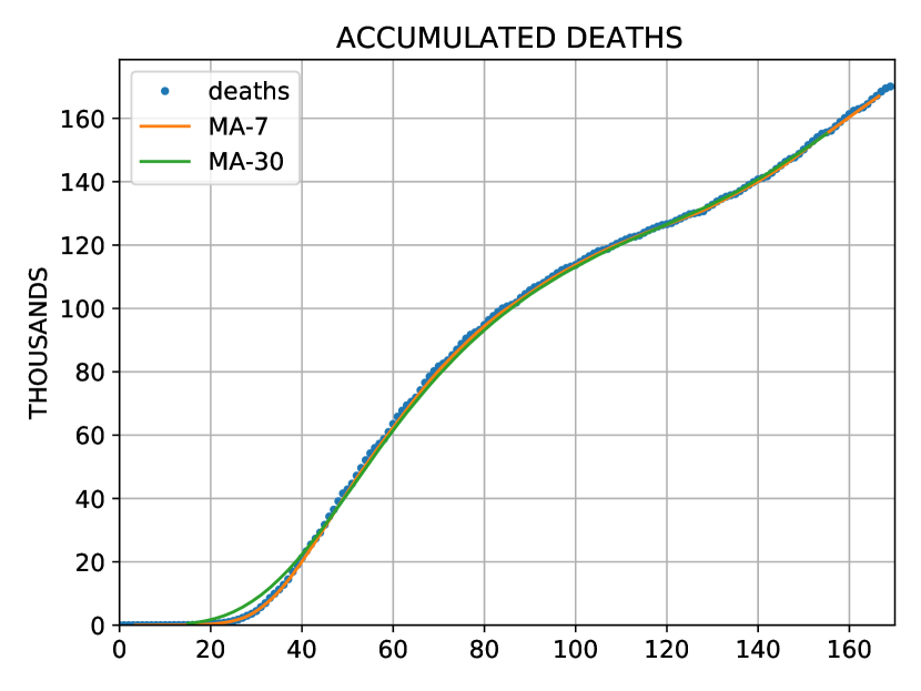
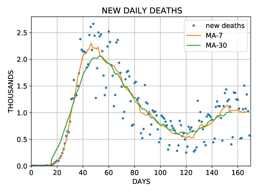
Figure 1: Accumulated and new daily deaths attributed to COVID–19 in the United States from 01/22/2020 through 08/16/2020 [12]. Day $0$ corresponds to the first day in this range in which a non-zero number of deaths was reported. Also shown is the result of the centered moving average with periods of $7$ and $30$ days. Note the large lags introduced by smoothing.

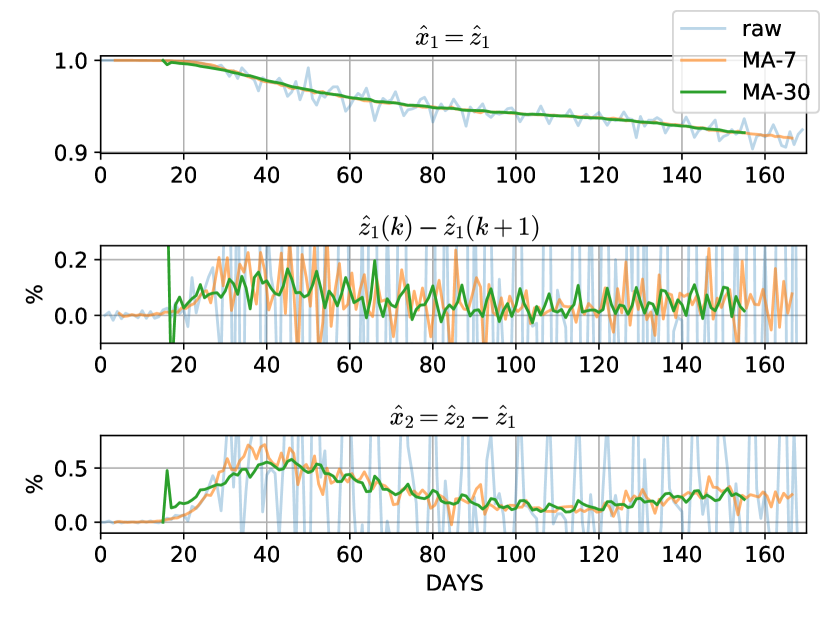
Figure 2: Estimates $\hat{x}_{1}=\hat{z}_{1}$ and $\hat{x}_{2}=\hat{z}_{2}-\hat{z}_{1}$ produced by the filter (22)–(28) for United States data from Fig. 1 for raw and centered moving averages with periods $7$ and $30$ days. Note how $\hat{x}_{1}=\hat{z}_{1}$ is not monotically decreasing, and $\hat{x}_{2}=\hat{z}_{2}-\hat{z}_{1}$ and $\hat{z}_{1}(k)-\hat{z}_{1}(k+1)$ often become negative, even after smoothing.

One problem with the above approach is that, in the presence of noise, there are no guarantees that the estimated variables $\hat{z}_{1}(k)$ and $\hat{z}_{2}(k)$ satisfy the structural constraints (21). Take for example the series of accumulated COVID-19 deaths in the United States shown in Fig. 1 obtained from the COVID-19 Data Repository by the Center for Systems Science and Engineering (CSSE) at Johns Hopkins University [12]. The corresponding estimates $\hat{z}_{1}$ and $\hat{z}_{2}$ and the key differences $\hat{z}_{1}(k)-\hat{z}_{1}(k+1)$ and $\hat{z}_{2}(k)-\hat{z}_{1}(k)$ are shown in Fig. 2. Note how these estimates do not satisfy (21). What this means is that the resulting $\hat{R}$ estimate (22) will experience wild swings and even take negative or very large values. In the example in Fig. 3, even the highly smoothed $30$-day moving average estimate swings below $0$ and above $5$. The raw and $7$-day moving average estimates are basically useless.

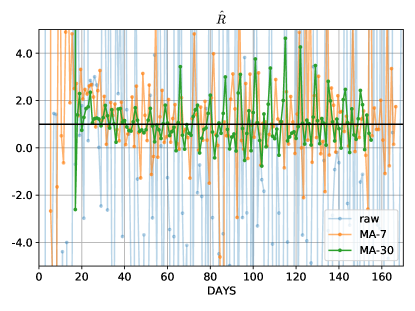
Figure 3: Unconstrained estimation of $R$ produced by the filter (22)–(28) corresponding to the United States deaths in Fig. 1 based on raw and centered moving average with periods of $7$ and $30$ days. All estimates display wide excursion range that take negative and large positive values.

While smoothing the input does improve the quality of the estimates, it does so at the expense of unavoidable loss of information as well as additional lags from filtering. Indeed, the authors of [2] explicitly mention that the above procedure should be fed a smoothed out version of the signal $y(k)$. Related approaches, such as [3], also seem to rely heavily on smoothing. These difficulties are the main motivation for the alternative constrained approach to be introduced in the next section.

This section is closed by presenting a property that is not apparent in [2], given in the following proposition.

Proposition 1.

For $k\geq 2$ the estimate

$$\hat{R}(k) =\frac{\hat{z}_{1}(k)-\hat{z}_{1}(k+1)}{\gamma(\hat{z}_{2}(k)-\hat{z}_{1}(k))}$$ (29)

in which $\hat{z}_{1}$ and $\hat{z}_{2}$ are the components of the output of the time-invariant linear filter (23)–(26) driven by the input (27) is independent of the value of fatality rate, $\delta$.

Proof.

Use linearity to write

$$\hat{z}(k) =\bar{z}(k)-\delta^{-1}\tilde{z}(k)$$

in which $\bar{z}$ and $\tilde{z}$ are such that

$$\bar{x}(k+1)=A\,\bar{x}(k)+B,\\ \bar{z}(k)=C\,\bar{x}(k)+D,\quad\bar{x}(0)=x_{0},$$

and

$$\tilde{x}(k+1)=A\,\tilde{x}(k)+B\,y(k),\\ \tilde{z}(k)=C\,\tilde{x}(k)+D\,y(k),\quad\tilde{x}(0)=0.$$

Then

$$\hat{R}(k) =\frac{\bar{z}_{1}(k)-\bar{z}_{1}(k+1)-\delta^{-1}(\tilde{z}_{1}(k)-\tilde{z}_{1}(k+1))}{\gamma\left(\bar{z}_{2}(k)-\bar{z}_{1}(k)-\delta^{-1}(\tilde{z}_{2}(k)-\tilde{z}_{1}(k))\right)}.$$

Because $A^{i}=0$, $i\geq 2$ and $B+AB=Ce+D=e$, where $e\in\mathbb{R}^{2}$ is a vector of ones, for any $k\geq 2$,

$$\bar{z}(k) =C\bar{x}(k)+D=\bar{x}(k)=A^{k}x_{0}+\sum_{i=0}^{k-1}A^{i}B=e.$$

Because $\bar{z}_{1}(k)=\bar{z}_{1}(k+1)=\bar{z}_{2}(k)=1$ it follows that

$$\hat{R}(k) =\frac{-\delta^{-1}(\tilde{z}_{1}(k)-\tilde{z}_{1}(k+1))}{-\delta^{-1}\gamma(\tilde{z}_{2}(k)-\tilde{z}_{1}(k))}=\frac{\tilde{z}_{1}(k)-\tilde{z}_{1}(k+1)}{\gamma(\tilde{z}_{2}(k)-\tilde{z}_{1}(k))}$$

is independent of $\delta$ for $k\geq 2$. ∎

IV Constrained Estimation

Some basic properties of the variables in the SRIDC model were listed in (21). In this section an alternative method for estimating the model variables and the time-varying parameter $R(k)$ will be introduced that allows one to enforce such and other constraints.

Consider the auxiliary linear time-invariant system

$$z_{1}(k+1) =z_{1}(k)-u(k)$$ (30)

$$z_{2}(k+1) =z_{2}(k)-\gamma\,z_{2}(k)+\gamma z_{1}(k)$$ (31)

$$z_{3}(k+1) =z_{3}(k)-\theta\,(z_{3}(k)-z_{2}(k))$$ (32)

in which $u(k)$ is an input to be determined. Equations (17)–(19) and (30)–(32) will have the exact same trajectories if they have the same initial conditions and

$$u(k) =\gamma\,R(k)(z_{2}(k)-z_{1}(k)).$$ (33)

This means that instead of estimating $R(k)$ from the nonlinear model (17)–(19) it is possible to use (33) to calculate

$$\hat{R}(k) =\frac{\hat{u}(k)}{\gamma\left(\hat{z}_{2}(k)-\hat{z}_{1}(k)\right)},$$ (34)

in which the input $\hat{u}$ and the variables $\hat{z}_{1}$ and $\hat{z}_{2}$ are estimated from the linear time-invariant model (30)–(32).

As it will be seen shortly, this alternative approach has several advantages. First, the resulting estimation problem is a convex problem that can be solved efficiently even with large number of data points. Second, the basic constraints (21) are all linear constraints that can be easily incorporated to the problem without compromising convexity. Third, it is possible to add constraints that will control the range of $R$ and its derivative, $\dot{R}$, as well as explicitly promote smoothness of the estimates.

In order to arrive at the desired problem formulation first introduce the estimator

$$\hat{x}(k+1) =A\,\hat{x}(k)+B\,\hat{u}(k)$$ (35)

in which

$$A=\begin{bmatrix}1&0&0\\ \gamma&(1-\gamma)&0\\ 0&\theta&(1-\theta)\end{bmatrix},\\ B=\begin{bmatrix}-1\\ 0\\ 0\end{bmatrix},\qquad\hat{x}(k)=\begin{pmatrix}\hat{z}_{1}(k)\\ \hat{z}_{2}(k)\\ \hat{z}_{3}(k)\\ \end{pmatrix}.$$ (36)

Equations (35)–(36) correspond to a state-space representation of (30)–(32) if $\hat{u}(k)=u(k)$, $\hat{x}(k)=x(k)$, and $\hat{x}(0)=x(0)$. Consider also the measurement (20) and

$$\hat{y}(k) =1+C\,\hat{x}(k), C =\begin{bmatrix}0&0&-1\end{bmatrix}.$$ (37)

Note that if $\hat{u}(k)=u(k)$ and $\hat{x}(0)=x(0)$ then $\delta\,\hat{y}(k)=y(k)$. This motivates the introduction of the cost function

$$\phi_{y}(w) =\frac{1}{N}\sum_{k=0}^{N-1}q(k)\left(y(k)-w(k)\right)^{2}$$ (38)

and the associated optimal estimation problem

$$\min_{\hat{y},\hat{x},\hat{u}} \phi_{y}(\delta\,\hat{y})$$ (39)

s.t. $$\hat{x}(k+1)=A\hat{x}(k)+B\hat{u}(k)$$

$$\hat{y}(k)=1+C\hat{x}(k)$$

$$\hat{u}(k)\geq 0,\quad k=0,\cdots,N-1$$

$$(\hat{x},\hat{u})\in\Omega$$

in which $\Omega$ is a constraint set that will be detailed below. In this paper, $\Omega$ will be comprised of linear constraints, hence Problem (39) will be a convex optimization problem [11].

The objective of Problem (39) is to produce a non-negative input $\hat{u}(k)$ that minimizes the weighted sum of squares of the error between the available measurement $y(k)$, in this case the deaths, and $\delta\,\hat{y}(k)$ produced by the dynamic model (35)–(36), in the presence of the additional convex constraints expressed in the set $\Omega$.

The weighting function $q(k)$ can be used to reflect the uncertainty level of each measurement. For example, under the assumption that the measurement noise can be modeled as a zero-mean and Gaussian white noise process a natural choice would be $q(k)=v(k)^{-1}$, where $v(k)$ is the variance of the measurement error at time $k$ [17]. The above problem is a variation on a standard finite-horizon linear quadratic optimal control problem [18].

The non-negativity constraint on $\hat{u}(k)$ follows from one of the basic constraints in (21). Indeed $\hat{u}(k)=\hat{z}_{1}(k)-\hat{z}_{1}(k+1)\geq 0$. The remaining constraints in (21) can be expressed in the form

$$\Omega_{b}=\big{\{}(\hat{x},\hat{u}):\quad 0\leq\hat{x}(k)\leq 1,\\ F\hat{x}(k)\leq 0,\quad k=0,\cdots,N\big{\}},$$

in which the matrix

$$F =\begin{bmatrix}1&-1&0\\ 0&1&-1\end{bmatrix}.$$

IV-A Constraints on $R$ and $\dot{R}$

Constraints on the estimates of $R$ and $\dot{R}$ can be translated as constraints on $\hat{x}$ and $\hat{u}$. The constraints discussed in this section implicitly assume that $z_{2}>z_{1}$, which will be the case whenever $z_{2}-z_{1}=x_{2}>0$, that is whenever the number of infected is still positive.

If lower- and upper-bounds on the value of $R\in[\underline{R},\overline{R}]$ are available then the same constraint applied on the estimate (34) can be translated as

$$\gamma\underline{R}(\hat{z}_{2}(k)-\hat{z}_{1}(k))\leq\hat{u}(k)\leq\gamma\overline{R}\,(\hat{z}_{2}(k)-\hat{z}_{1}(k))$$

which can be represented by the set of linear constraints

$$\Omega_{R}=\big{\{}(\hat{x},\hat{u}):\quad\gamma\underline{R}\,G\hat{x}(k)\leq\hat{u}(k)\leq\gamma\overline{R}\,G\hat{x}(k),\\ k=0,\cdots,N-1\big{\}}$$

in which the matrix

$$G =\begin{bmatrix}-1&1&0\\ \end{bmatrix}.$$

Note how important is to formulate the estimation problem in terms of $R$ rather than $\beta$: the equivalent constraints in $\beta$ would be nonlinear while the ones in $R$ are linear.

It is also useful to constrain the derivative of $R$, that is $\dot{R}$, which is easier to manipulate in the continuous-time version of model (30)–(32), namely

$$\dot{z}_{1} =-u,$$

$$\dot{z}_{2} =-\gamma\,(z_{2}-z_{1}),$$

$$\dot{z}_{3} =-\theta\,(z_{3}-z_{2}),$$

from which

$$R =\frac{u}{\gamma(z_{2}-z_{1})}, \dot{R} =\frac{\dot{u}(z_{2}-z_{1})-(\dot{z}_{2}-\dot{z}_{1})u}{\gamma(z_{2}-z_{1})^{2}}.$$ and

If $R\in[\underline{R},\overline{R}]$ then

$$\frac{\dot{u}-\gamma(\dot{z}_{2}-\dot{z}_{1})\overline{R}}{\gamma(z_{2}-z_{1})}\leq\dot{R}\leq\frac{\dot{u}-\gamma(\dot{z}_{2}-\dot{z}_{1})\underline{R}}{\gamma(z_{2}-z_{1})}$$

Therefore, since $z_{2}>z_{1}$, if

$$(\dot{z}_{2}-\dot{z}_{1})\overline{R}+\underline{\dot{R}}(z_{2}-z_{1})\leq\gamma^{-1}\dot{u}\leq\\ (\dot{z}_{2}-\dot{z}_{1})\underline{R}+\overline{\dot{R}}(z_{2}-z_{1}),$$

then $\dot{R}\in[\underline{\dot{R}},\overline{\dot{R}}]$. These inequalities can be expressed approximately in terms of the discrete-time variables in model (30)–(32) upon substituting

$$\dot{u} \approx u(k+1)-u(k),$$

$$\dot{z}_{2}-\dot{z}_{1} \approx z_{2}(k+1)-z_{1}(k+1)-z_{2}(k)+z_{1}(k)$$

$$\qquad\qquad=u(k)+\gamma(z_{1}(k)-z_{2}(k)),$$

leading to the constraints on the estimates

$$(\gamma\overline{R}-\underline{\dot{R}})\hat{z}_{1}(k)-(\gamma\overline{R}-\underline{\dot{R}})\hat{z}_{2}(k)+\overline{R}\hat{u}(k)\leq\\ \gamma^{-1}(\hat{u}(k+1)-\hat{u}(k))\leq\\ (\gamma\underline{R}-\overline{\dot{R}})\hat{z}_{1}(k)-(\gamma\underline{R}-\overline{\dot{R}})\hat{z}_{2}(k)+\underline{R}\hat{u}(k).$$

An extension is to have bounds on $\dot{R}(k)$ that vary depending on $k$. This is especially useful to capture the higher uncertainties associated with the beginning of the pandemic, a period when noisy date might suggest a wider variation on $R$ and hence its derivative. Such time dependent constraint can be represented by the set

$$\Omega_{\dot{R}}=\big{\{}(\hat{x},\hat{u}):\\ \gamma\underline{H}(k)\hat{x}(k)+\gamma\overline{R}u(k)\leq\hat{u}(k+1)-\hat{u}(k),\\ \hat{u}(k+1)-\hat{u}(k)\leq\gamma\overline{H}(k)\hat{x}(k)+\gamma\underline{R}u(k),\\ k=0,\cdots,N-1\big{\}}$$

in which

$$\underline{H}(k) =\begin{bmatrix}(\gamma\overline{R}-\underline{\dot{R}}(k))&-(\gamma\overline{R}-\underline{\dot{R}}(k))&0\end{bmatrix},$$

$$\overline{H}(k) =\begin{bmatrix}(\gamma\underline{R}-\overline{\dot{R}}(k))&-(\gamma\underline{R}-\overline{\dot{R}}(k))&0\end{bmatrix},$$

and $\dot{R}(k)\in[\underline{\dot{R}}(k),\overline{\dot{R}}(k)]$. Even though the above constraints, having been ported from the continuous-time model to the discrete-time model, are approximations, they are very effective, as it will be illustrated by examples later.

IV-B Initial Condition

It is not necessary to have an estimate of the initial condition, $\hat{x}(0)$, to solve Problem (39). The optimal solution will provide a suitable estimate of the initial condition. However, it is interesting to note that it is always possible to chose $\hat{x}(0)$ so that $\hat{y}(k)=\delta^{-1}y(k)$ for $k=\{0,1,2\}$ without further constraining $\hat{u}(k)$. Indeed, verify that

$$CB=CAB=0$$

and that

$$\begin{bmatrix}C\\ CA\\ CA^{2}\end{bmatrix}x(0) =\delta^{-1}\begin{pmatrix}y(0)\\ y(1)\\ y(2)\end{pmatrix}-e,$$

in which $e\in\mathbb{R}^{3}$ is a vector of ones. Because the above coefficient matrix is the Observability Matrix [18] associated with the pair $(A,C)$ which, for $A$ and $C$ from (36) and (37), is square and non-singular, one can calculate

$$\mu_{0} =\begin{bmatrix}C\\ CA\\ CA^{2}\end{bmatrix}^{-1}\begin{pmatrix}\delta^{-1}y(0)-1\\ \delta^{-1}y(1)-1\\ \delta^{-1}y(2)-1\end{pmatrix}.$$ (40)

As discussed above, fixing $\hat{x}(0)=\mu_{0}$ may not lead to the best possible overall estimate but one could incorporate such knowledge, if desired, by adding the function

$$\phi_{0}(\hat{x}(0))=\|\Pi(\hat{x}(0)-\mu_{0})\|_{2}^{2}$$ (41)

to the cost of Problem (39). Matrix $\Pi$ can be used to weigh the user confidence on the estimate $\mu_{0}$. The examples shown in the present paper do not make use of (41). However, weighing prior knowledge on the initial condition can be useful in the presence of additional measurements, to be discussed in Section IV-G.

IV-C Smoothness Cost

The estimation Problem (39) takes the form of a finite horizon optimal control problem [18]. However, a typical finite horizon optimal control problems is often formulated with two more types of costs: a penalty on the terminal state and a direct penalty on the control cost, typically a measure of the energy of the signal $\hat{u}(k)$. There are lots of good reasons for such penalties to be part of the cost [18]. Here a penalty on the signal $\hat{u}$ will be used as a way to promote smoothness of the estimates.

Consider first a penalty on the terminal state. As it is typical of discrete-time dynamic systems, the effects of the input signal $\hat{u}$ may not appear in the output signal $\hat{y}$ until a number of iterations has taken place. In the case of the model (35)–(37), since $BC=BAC=0$, it takes at least two iterations for the input to show up at the output. That is, the value of the input $\hat{u}(k)$ will only appear in the output $\hat{y}(k+2)$. See also the discussion in Section IV-B. This means that the final two values of $\hat{u}(k)$ have no effect on the cost function of Problem (39). However, they will have an effect on the state, which ultimately affects the estimate $\hat{R}(k)$. This means that the last two estimates of $\hat{R}(k)$ should probably not be trusted. This is equivalent to the two-step delay of the unconstrained estimator discussed earlier in Section III.

In a typical control problem, a terminal cost ensures that, even in the absence of measurements that can help determine $u(k)$ on those final instants, the final state is steered toward a desired state. However, in Problem (39) there does not seem to be a clear choice of a desired state, unless the analysis pertains to past events in which the disease has already reached equilibrium and information on the equilibrium state is available. For this reason, in the context of the COVID-19 epidemic, no terminal constraint shall be imposed.

As for a running cost on the signal $\hat{u}$, solutions to Problem (39) are likely to still produce a signal $\hat{u}(k)$ that can have significant variations, even after imposing the constraints discussed so far. Indeed, the very nature of the Problem (39) is to produce an optimal $\hat{u}(k)$ that will do its best to capture the variations implied by a changing $y(k)$. However, as far as estimating $R(k)$, it may not be important to capture every single variation, but rather to smooth out the trends. This goal is achieved by adding the smoothness cost

$$\phi_{s}(\hat{u})=\\ \frac{1}{N\!-\!2}\left(r(0)|\hat{u}(0)|^{2}+\!\sum_{k=1}^{N-3}r(k)\left|\hat{u}(k)-\hat{u}(k-1)\right|^{2}\right)$$ (42)

which penalizes the total variations of $\hat{u}$ measured at consecutive samples. This cost function promotes smoothness of $\hat{u}(k)$, which in turns promotes smoothness of $\hat{R}(k)$, as it will be seen in the examples. Note also that (42) does not penalize the last two values of $\hat{u}(k)$ since, as discussed above, they do not affect the measurements at $k=N-2$ and $N-1$.

IV-D Trading-off Accuracy Versus Smoothness

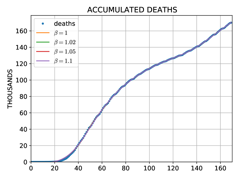
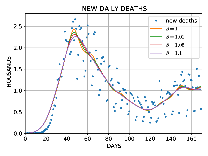
Figure 4: Accumulated and new daily deaths attributed to COVID–19 in the United States from 01/22/2020 through 08/16/2020 [12]. Day $0$ corresponds to the first day in this range in which a non-zero number of deaths was reported. Also shown is the corresponding constrained estimates produced by solving Problem (43) for various values of $\beta$. The solution to Problem (39) corresponds to $\beta=1$.

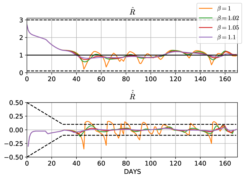
Figure 5: Constrained estimates produced by solving Problem (43) for various values of $\beta$ for the data in Fig. 4. The constraints imposed on the estimated $R$ and $\dot{R}$ are shown by the dashed lines.

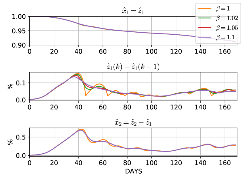
Figure 6: Constrained estimates $\hat{x}_{1}=\hat{z}_{1}$ and $\hat{x}_{2}=\hat{z}_{2}-\hat{z}_{1}$ produced by solving Problem (43) for various values of $\beta$ for the data in Fig. 4. Note how $\hat{x}_{1}=\hat{z}_{1}$ is monotonically decreasing and remains below one, and $\hat{x}_{2}=\hat{z}_{2}-\hat{z}_{1}$ and $\hat{z}_{1}(k)-\hat{z}_{1}(k+1)$ remain positive.

This section will illustrate how the optimization problem and the constraints discussed so far can be used to produce smooth estimates of the SIRDC model variables and the parameter $R$. Let us start by solving Problem (39) for the United States data shown before in Fig. 1. The following constant parameters were used:

$$\gamma =0.2, \theta =0.1, \delta =0.065, \overline{R} =3, \underline{R} =0.1,$$

with the constraint set

$$\Omega=\Omega_{b}\cap\Omega_{R}\cap\Omega_{\dot{R}}.$$

The derivative of $R$, $\dot{R}$, was constrained by the time-dependent bounds

$$\underline{\dot{R}}(k) =-\overline{\dot{R}}(k),$$

$$\overline{\dot{R}}(k) =\begin{cases}0.5(k/30)+0.1(1-k/30),&k\leq 30,\\ 0.1,&k>30,\end{cases}$$

which allows larger variations at the beginning of the epidemic, and a constant weight

$$q(k) =1, k =0,\cdots,N-1,$$

was used in the cost function. No penalty on the initial condition was imposed.

The estimated deaths and new daily deaths and the corresponding estimates for $R$ and $\dot{R}$ obtained by Problem (39) are shown in Fig. 4 and 6, with the label $\beta=1$. Note how the constraints on $R$ are enforced at all times while the constraints on $\dot{R}$ are approximately enforced, as discussed in Section IV-A. All numerical examples in this paper were formulated using CVXPY [19] and solved using MOSEK’s conic solver [20].

Enforcing the constraints on the model variables and parameters during the estimation process ensures that the estimates produced are much better behaved and smoother when compared with the estimates obtained by the unconstrained estimation methods of Section III. The smoothness of the estimate can be further enhanced by incorporating a smoothness cost as discussed in Section IV-C. As it is customary, one could modify Problem (39) by replacing its cost function by

$$\phi_{y}(\delta\,\hat{y})+\eta\,\phi_{s}(\hat{u})$$

where $\eta>0$ is a penalty parameter. The correct tuning of the parameter $\eta$ can however be tricky. Instead, perform the following two step procedure:

1. Solve the convex optimization Problem (39) and determine its global optimal solution and cost. Let $\rho^{*}$ be the minimal cost.

2. Select $\beta\geq 1$ and solve the convex quadratic optimization problem with linear and convex quadratic constraints

   $$\min_{\hat{y},\hat{x},\hat{u}} \delta^{2}\,\phi_{s}(\hat{u})$$ (43)

   s.t. $$\hat{x}(k+1)=A\hat{x}(k)+B\hat{u}(k)$$

   $$\hat{y}(k)=C\hat{x}(k)+Er(k)$$

   $$\hat{u}(k)\geq 0,\quad k=0,\cdots,N-1$$

   $$(\hat{x},\hat{u})\in\Omega$$

   $$\phi_{y}(\delta\,\hat{y})\leq\beta\,\rho^{*}$$

The reason for scaling the cost function by the square of the fatality rate $\delta$ will be made clear in Section IV-E.

The parameter $\beta\geq 1$ can be interpreted as how much accuracy one is willing to trade for smoothness. Indeed when $\beta=1$, Problems (39) and (43) admit the exact same optimal solution. However, as $\beta$ increases, smoother solutions are possible at the expense of a higher estimation error. In the case of the United States COVID-19 data, the estimates produced with $\beta=\{1.02,1.05,1.1\}$ are also shown in Figs. 4–6.

The impact of the value of $\beta$ is still data dependent. Indeed, the more noise is present in the data the less smooth one would expect the solution to Problem (39) to be, and the higher one might need to set $\beta$ for the desired level of smoothness. Note also that as the penalty $\beta$ increases the constraints on $R$ and its derivative becomes less and less active. However, solving Problem 39 without these constraints would make the choice of $\beta$ much more difficult, as the value of the cost function of Problem 39 is allowed to be reduced further by increasingly less smooth solutions. By enforcing these constraints earlier in Problem (39) it is found that a choice of $\beta\in[1,2]$ is enough to produce suitable solutions for data from diverse countries, to be presented in Section V.

IV-E Independence of the Fatality Rate

The constrained estimator obtained as the solution to the optimization problems (39) and (43) enjoy the same independence of the fatality rate, $\delta$, as the unconstrained estimator from Section III. The following result is analogous to Proposition 1. Its proof reveals the need for the scaling of the objective function in Problem (43).

Proposition 2.

The estimate

$$\hat{R}(k) =\frac{\hat{u}(k)}{\gamma(\hat{z}_{2}(k)-\hat{z}_{1}(k))}$$ (44)

in which $\hat{z}_{1}$ and $\hat{z}_{2}$ are obtained as solutions to Problem (39) or Problem (43) is independent of the value of the fatality rate, $\delta$.

Proof.

Let $\hat{y}_{\delta}$, $\hat{x}_{\delta}$ and $\hat{u}_{\delta}$ be the optimal solution to Problem (39) for some $\delta>0$, that is

$$(\hat{y}_{\delta},\hat{x}_{\delta},\hat{u}_{\delta}) =\arg\min_{(\hat{y},\hat{x},\hat{u})\in\hat{\Omega}}\phi_{y}(\delta\,\hat{y})$$

in which

$$\hat{\Omega}=\big{\{}(\hat{y},\hat{x},\hat{u}):\quad\hat{x}(k+1)=A\hat{x}(k)+B\hat{u}(k),\\ \hat{y}(k)=1+C\hat{x}(k),\quad\hat{u}(k)\geq 0,\quad k=1,\cdots,N-1,\\ (\hat{x},\hat{u})\in\Omega=\Omega_{b}\cap\Omega_{R}\cap\Omega_{\dot{R}}\big{\}},$$

for $A$, $B$, and $C$ from (36)–(37). Since $\delta$ only affects the value of the cost function, there will exist an optimal solution for any $\delta>0$ as long as $\hat{\Omega}\neq\emptyset$.

Now let $0<\lambda\leq 1$, and calculate

$$\hat{x}_{\lambda}(k+1)=A\,\hat{x}_{\lambda}(k)+B\,\hat{u}_{\lambda}(k),\\ \bar{x}_{\lambda}(0)=\lambda\,\hat{x}_{\delta}(0)+(1-\lambda)\,e,\quad\hat{u}_{\lambda}(k)=\lambda\,\hat{u}_{\delta}(k),$$

in which $e\in\mathbb{R}^{3}$ is a vector of ones, and use the fact that $A^{k}e=e$, $k=0,1,\cdots$, to show that

$$\hat{x}_{\lambda}(k) =\lambda\,\hat{x}_{\delta}(k)+(1-\lambda)\,e.$$

Since $0\leq\hat{x}_{\delta}(k)\leq e$ and $0<\lambda\leq 1$

$$0\leq\hat{x}_{\lambda}(k)\leq e.$$

Furthermore $Fe=0$ so that

$$F\hat{x}_{\lambda}(k)=\lambda\,F\hat{x}_{\delta}(k)\leq 0$$

and $\hat{x}_{\lambda}(k)\in\Omega_{b}$. Likewise, because $G\,e=0$, $\underline{H}(k)\,e=\overline{H}(k)\,e=0$, $\hat{x}_{\lambda}(k)\in\Omega_{R}\cap\Omega_{\dot{R}}$. Finally, using the fact that $C\,e=-1$,

$$\hat{y}_{\lambda}(k)=1+C\hat{x}_{\lambda}(k)=\\ 1+(1-\lambda)\,Ce+\lambda\,C\hat{x}_{\delta}(k)=\lambda\,\hat{y}_{\delta}(k),$$

from which one concludes that $(\hat{y}_{\lambda},\hat{x}_{\lambda},\hat{u}_{\lambda})\in\hat{\Omega}$.

Note that for any $y$, $z$ and $0<\lambda\leq 1$ it is true that

$$N\phi_{y}(\lambda^{-1}z) =\|y-\lambda^{-1}z\|_{Q}^{2}$$

$$\geq\lambda^{-1}\left(\|z\|_{Q}^{2}-2\,z^{T}Qy\right)+\|y\|_{Q}^{2}$$

$$\geq\|y-z\|_{Q}^{2}=N\phi_{y}(z),$$

in which $Q=\operatorname{diag}(q(0),\cdots,q(N-1))$ and $\|x\|_{Q}^{2}=x^{T}Q\,x$, so that

$$\min_{(\hat{y},\hat{x},\hat{u})\in\hat{\Omega}}\phi_{y}(\lambda^{-1}\delta\,\hat{y}) \geq\min_{(\hat{y},\hat{x},\hat{u})\in\hat{\Omega}}\phi_{y}(\delta\,\hat{y})=\phi_{y}(\delta\,\hat{y}_{\delta}).$$

On the other hand, since $(\hat{y}_{\lambda},\hat{x}_{\lambda},\hat{u}_{\lambda})\in\hat{\Omega}$,

$$\min_{(\hat{y},\hat{x},\hat{u})\in\hat{\Omega}}\phi_{y}(\lambda^{-1}\delta\,\hat{y})\leq\phi_{y}(\lambda^{-1}\delta\,\hat{y}_{\lambda})=\phi_{y}(\delta\,\hat{y}_{\delta}).$$

Combining these two inequalities it is possible to conclude that

$$\min_{(\hat{y},\hat{x},\hat{u})\in\hat{\Omega}}\phi_{y}(\lambda^{-1}\delta\,\hat{y})=\phi_{y}(\delta\,\hat{y}_{\delta}),\quad\text{for all }0<\lambda\leq 1,$$

which proves the proposition for Problem (39) since the above discussion holds for any small enough $\delta>0$.

As for Problem (43), the above discussion means that the constraint

$$\phi_{y}(\delta\,\hat{y})\leq\beta\,\rho^{*}$$

will be unaffected by the choice of $\delta$ since $\rho^{*}$ is independent of $\delta$. Therefore, an argument similar to the one used for Problem (43) in which

$$(\hat{y}_{\delta},\hat{x}_{\delta},\hat{u}_{\delta})=\arg\min_{(\hat{y},\hat{x},\hat{u})\in\hat{\Omega}_{s}}\delta^{2}\,\phi_{s}(\hat{u}),\\ \hat{\Omega}_{s}=\{(\hat{y},\hat{x},\hat{u})\in\hat{\Omega}:\quad\phi_{y}(\delta\,\hat{y})\leq\beta\,\rho^{*}\},$$

leads to

$$\min_{(\hat{y},\hat{x},\hat{u})\in\hat{\Omega}_{s}}\!\lambda^{-2}\delta^{2}\,\phi_{s}(\hat{u})\geq\!\min_{(\hat{y},\hat{x},\hat{u})\in\hat{\Omega}_{s}}\!\delta^{2}\,\phi_{s}(\hat{u})=\delta^{2}\,\phi_{s}(\hat{u}_{\delta})$$

for all $0<\lambda\leq 1$ and, since $(\hat{y}_{\lambda},\hat{x}_{\lambda},\hat{u}_{\lambda})\in\hat{\Omega}_{s}$,

$$\min_{(\hat{y},\hat{x},\hat{u})\in\hat{\Omega}_{s}}\!\lambda^{-2}\delta^{2}\,\phi_{s}(\hat{u})\leq\lambda^{-2}\delta^{2}\,\phi_{s}(\hat{u}_{\lambda})=\delta^{2}\,\phi_{s}(\hat{u}_{\delta}),$$

from which

$$\min_{(\hat{y},\hat{x},\hat{u})\in\hat{\Omega}_{s}}\!\lambda^{-2}\delta^{2}\,\phi_{s}(\hat{u})=\delta^{2}\,\phi_{s}(\hat{u}_{\delta}),$$

for all $0<\lambda\leq 1$, as in Problem (39). ∎

IV-F Problem Summary

The optimization problems (39) and (43) are convex quadratic programs with linear and convex quadratic constraints. It is possible to take advantage of the linear nature of the equations (35)–(36) to propagate the state evolution as a function of the inputs and the initial condition. That is the entire state $\hat{x}(k)$, $k=0,\cdots,N$, can be written as

$$\begin{pmatrix}\hat{x}(0)\\ \hat{x}(1)\\ \vdots\\ \hat{x}(N)\end{pmatrix} =\mathsf{T}\,\mathsf{x}, \mathsf{x} =\begin{pmatrix}\hat{x}_{0}\\ \hat{u}(0)\\ \hat{u}(1)\\ \vdots\\ \hat{u}(N-1)\end{pmatrix}$$

in which

$$\mathsf{T} =\begin{bmatrix}I&0&0&\cdots&0\\ A&B&0&\cdots&0\\ \vdots&\vdots&\vdots&\ddots&\vdots\\ A^{N}&A^{N-1}B&A^{N-2}B&\cdots&B\end{bmatrix}.$$

Using the above, one can write

$$\phi_{0}(\hat{x}(0))+\phi_{y}(\delta\,\hat{y})=\|\mathsf{Q}^{1/2}\left(\mathsf{A}\,\mathsf{x}-\mathsf{y}\right)\|_{2}^{2}$$

in which $\mathsf{Q}=\operatorname{diag}(q(0),\cdots,q(N-1))$ and

$$\mathsf{y} =\begin{pmatrix}\Pi\,\mu_{0}\\ y(0)-\delta\\ y(1)-\delta\\ \vdots\\ y(N-1)-\delta\end{pmatrix},$$

$$\mathsf{A} =\begin{bmatrix}\Pi&0&0&\cdots&0\\ \delta\,C&0&0&\cdots&0\\ \delta\,CA&\delta\,CB&0&\cdots&0\\ \vdots&\vdots&\vdots&\ddots&\vdots\\ \delta\,CA^{N-1}&\delta\,CA^{N-2}B&\delta\,CA^{N-3}B&\cdots&0\end{bmatrix}.$$

The cost function of Problem (39) is a special case in which $\Pi=0$.

Similar manipulations can convert the linear constraints $\Omega_{b}$ and $\Omega_{R}$ to the form

$$0\leq\mathsf{T}\,\mathsf{x} \leq 1, \mathsf{F}\,\mathsf{x} \leq 0, \gamma\,\underline{R}\,\mathsf{G}\,\mathsf{x} \leq\mathsf{I}\,\mathbf{x}\leq\gamma\,\overline{R}\,\mathsf{G}\,\mathsf{x},$$

in which $\mathsf{I}=\begin{bmatrix}0&I\end{bmatrix}$,

$$\mathsf{F} =\begin{bmatrix}F&0&0&\cdots&0\\ FA&FB&0&\cdots&0\\ \vdots&\vdots&\vdots&\ddots&\vdots\\ FA^{N}&FA^{N-1}B&FA^{N-2}B&\cdots&FB\end{bmatrix},$$

$$\mathsf{G} =\begin{bmatrix}G&0&0&\cdots&0\\ GA&GB&0&\cdots&0\\ \vdots&\vdots&\vdots&\ddots&\vdots\\ GA^{N-1}&GA^{N-2}B&GA^{N-3}B&\cdots&0\end{bmatrix}.$$

The constraints in $\Omega_{\dot{R}}$ can be reformulated as

$$\gamma\,\underline{\mathsf{H}}\,\mathsf{x} \leq\mathsf{D}\,\mathbf{x}\leq\gamma\,\overline{\mathsf{H}}\,\mathsf{x}$$

in which

$$\underline{\mathsf{H}} =\begin{bmatrix}\underline{H}(0)&\overline{R}&\cdots&0\\ \underline{H}(1)A&\underline{H}(1)B&\cdots&0\\ \vdots&\vdots&\ddots&\vdots\\ \underline{H}(N-1)A^{N-1}&\underline{H}(N-1)A^{N-2}B&\cdots&\overline{R}\end{bmatrix},$$

$$\overline{\mathsf{H}} =\begin{bmatrix}\overline{H}(0)&\underline{R}&\cdots&0\\ \overline{H}(1)A&\overline{H}(1)B&\cdots&0\\ \vdots&\vdots&\ddots&\vdots\\ \overline{H}(N-1)A^{N-1}&\overline{H}(N-1)A^{N-2}B&\cdots&\underline{R}\end{bmatrix},$$

$$\mathsf{D} =\begin{bmatrix}0&-1&1&\cdots&0\\ 0&0&-1&\cdots&0\\ \vdots&\vdots&\vdots&\ddots&\vdots\\ 0&0&0&\cdots&1\end{bmatrix}.$$

The above can be put together to reformulate Problem (39) as the following convex quadratic program with linear constraints

$$\min_{\mathsf{x}}\quad \|\mathsf{Q}^{1/2}\left(\mathsf{A}\,\mathsf{x}-\mathsf{y}\right)\|_{2}^{2}$$

s.t. $$0\leq\mathsf{T}\,\mathsf{x}\leq 1,\quad\mathsf{F}\,\mathsf{x}\leq 0,$$

$$\gamma\,\underline{R}\,\mathsf{G}\,\mathsf{x}\leq\mathsf{I}\,\mathbf{x}\leq\gamma\,\overline{R}\,\mathsf{G}\,\mathsf{x},$$

$$\gamma\,\underline{\mathsf{H}}\,\mathsf{x}\leq\mathsf{D}\,\mathbf{x}\leq\gamma\,\overline{\mathsf{H}}\,\mathsf{x}$$

Likewise, the cost $\phi_{s}$ can be expressed as

$$\phi_{s}(\hat{u}) =\|\mathsf{R}^{1/2}\,\mathsf{B}\,\mathsf{x}\|_{2}^{2}$$

in which $\mathsf{R}=\operatorname{diag}(r(0),\cdots,r(N-1))$,

$$\mathsf{B} =\begin{bmatrix}0&1&0&\cdots&0\\ 0&-1&1&\cdots&0\\ \vdots&\vdots&\vdots&\ddots&\vdots\\ 0&0&0&\cdots&1\end{bmatrix}.$$

This means that problem (43) can be formulated as the convex quadratic program with quadratic constraints

$$\min_{\mathsf{x}}\quad \delta^{2}\,\|\mathsf{R}^{1/2}\,\mathsf{B}\,\mathsf{x}\|_{2}^{2}$$

s.t. $$0\leq\mathsf{T}\,\mathsf{x}\leq 1,\quad\mathsf{F}\,\mathsf{x}\leq 0,$$

$$\gamma\,\underline{R}\,\mathsf{G}\,\mathsf{x}\leq\mathsf{I}\,\mathbf{x}\leq\gamma\,\overline{R}\,\mathsf{G}\,\mathsf{x},$$

$$\gamma\,\underline{\mathsf{H}}\,\mathsf{x}\leq\mathsf{D}\,\mathbf{x}\leq\gamma\,\overline{\mathsf{H}}\,\mathsf{x},$$

$$\|\mathsf{Q}^{1/2}\left(\mathsf{A}\,\mathsf{x}-\mathsf{y}\right)\|_{2}^{2}\leq\beta\,\rho^{*}$$

The above problems can be formulated and solved efficiently using modern convex optimization algorithms in stock desktop computers for problems with tens of thousands of variables and constraints.

IV-G Handling Additional Measurements

The proposed constrained optimization approach can be extended to handle additional measurements. For example, one could leverage testing data to estimate the current number of infected and resolving cases, that is to provide additional measurements of the model variables $x_{2}$ and $x_{3}$. By grouping these measurements into a vector $y(k)\in\mathbb{R}^{3}$ in which the first entry is the fraction of deaths, the second entry is the fraction of infected individuals, and the third entry is the fraction of resolving individuals, one can calculate the best constrained estimate by using the exact same estimator dynamic model as (35)–(36) with the extended measurement model

$$\hat{y}(k) =g+H\hat{x}(k), \!\!H =\begin{bmatrix}0&0&-\delta\\ -1&1&0\\ 0&-1&1\end{bmatrix}\!, \!\!g =\begin{pmatrix}\delta\\ 0\\ 0\end{pmatrix}\!,$$

resulting into the optimization problem

$$\min_{\hat{y},\hat{x},\hat{u}} \phi_{y}(\hat{y})$$ (45)

s.t. $$\hat{x}(k+1)=A\hat{x}(k)+B\hat{u}(k)$$

$$\hat{y}(k)=g+H\hat{x}(k)$$

$$\hat{u}(k)\geq 0,\quad k=0,\cdots,N-1$$

$$(\hat{x},\hat{u})\in\Omega$$

Note how the fatality rate has been incorporated into the matrix $H$ and vector $g$. It should not be expected that the independence property of Proposition 2 holds in the presence of the additional measurements since scaling the infected and resolving population to match a given fatality rate, as done in the proof of Proposition 2, will no longer preserve optimality. In fact, one might use the additional data to jointly estimate the parameter $\delta$.

Another possible extension that might be especially useful in the presence of additional measurement is the relaxation of the dynamic equality constraints in Problem (45) as a penalty function, as usually done in smoothing problems [17]. Additional nonlinear model features could also be added at the expense of loosing convexity of the overall optimization problem.

V Conclusions and Discussion

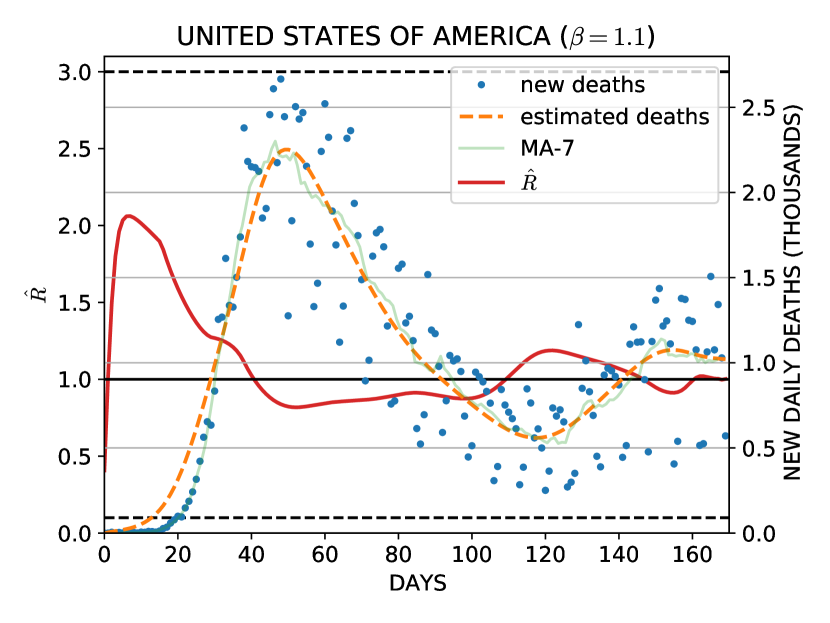
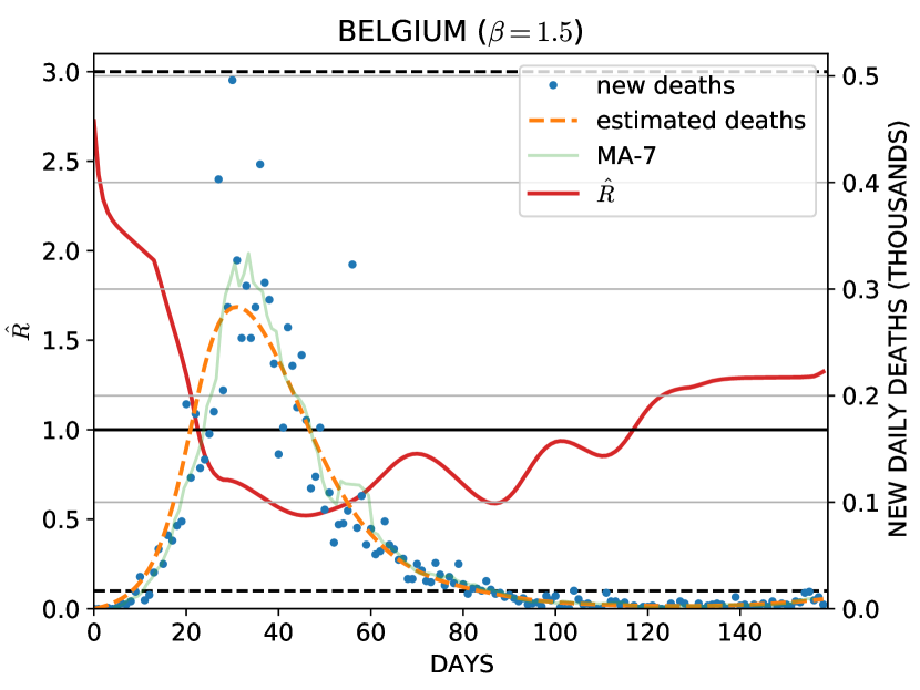
Figure 7: New daily deaths attributed to COVID–19 in the United States and Belgium from 01/22/2020 through 08/16/2020 [12] along with estimates for new deaths and $R$ produced by solving Problem (43). The value of $\beta$ used is shown in the legends. Also show for comparison is a $7$-day moving average of new deaths.

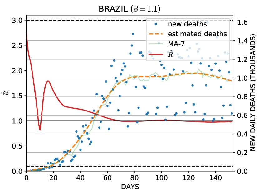
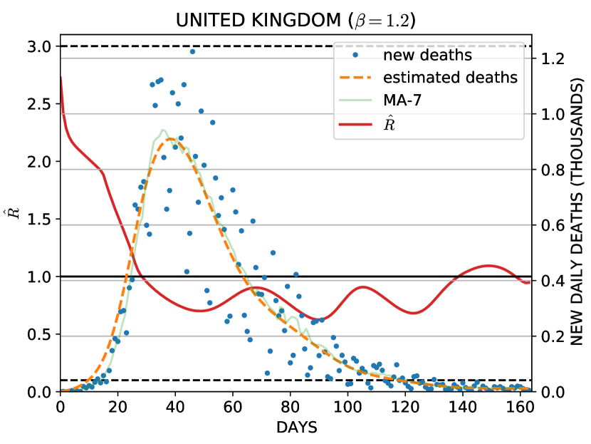
Figure 8: New daily deaths attributed to COVID–19 in the Brazil and the United Kingdom from 01/22/2020 through 08/16/2020 [12] along with estimates for new deaths and $R$ produced by solving Problem (43). The value of $\beta$ used is shown in the legends. Also show for comparison is a $7$-day moving average of new deaths.

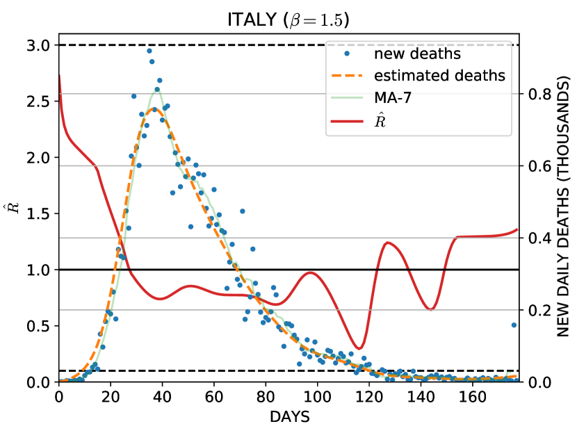
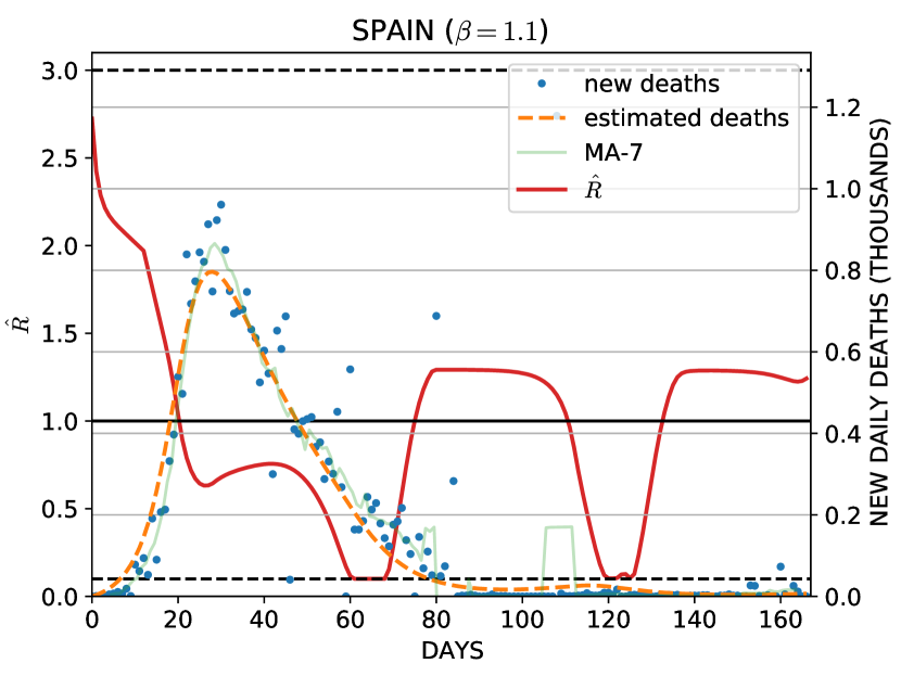
Figure 9: New daily deaths and $7$-day moving average attributed to COVID–19 in Italy and Spain from 01/22/2020 through 08/16/2020 [12] along with estimates for new deaths and $R$ produced by solving Problem (43). The value of $\beta$ used is shown in the legends. Also show for comparison is a $7$-day moving average of new deaths.

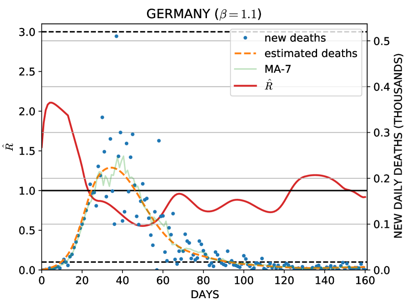
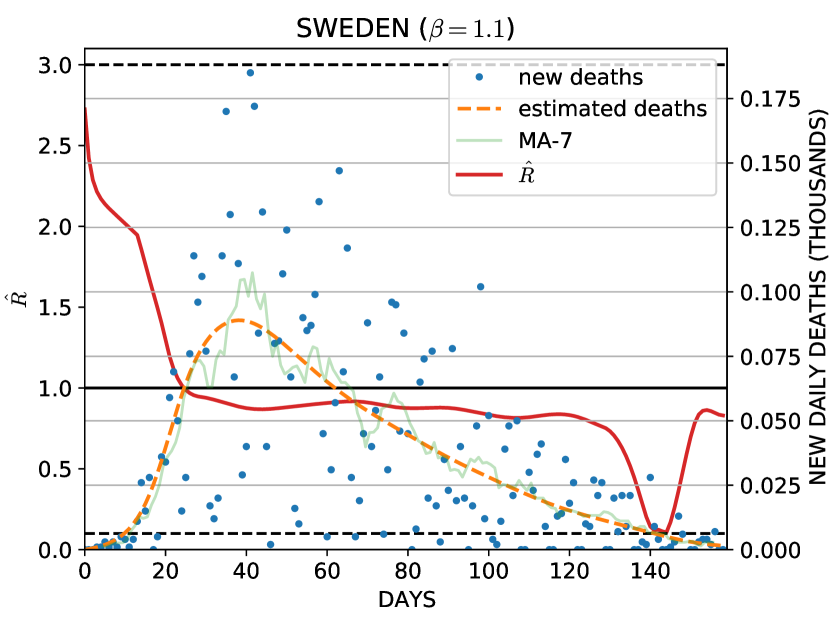
Figure 10: New daily deaths and $7$-day moving average attributed to COVID–19 in Germany and Sweden from 01/22/2020 through 08/16/2020 [12] along with estimates for new deaths and $R$ produced by solving Problem (43). The value of $\beta$ used is shown in the legends. Also show for comparison is a $7$-day moving average of new deaths.

The present paper has revisited unconstrained and proposed new constrained methods for estimation of the variables and time-varying parameters of compartmental models with application to the present COVID-19 epidemic. Even though the underlying model is nonlinear, a change of coordinates enables the estimation to be done using an auxiliary linear model that results in convex quadratic optimization problems which can be solved globally and very efficiently, as well as be applied to large data sets. The constrained method has been shown to preserve the physical properties of the model variables throughout the estimation. Through an additional penalty on the total variation of the estimates one can trade-off accuracy versus smoothness of the obtained estimates.

The paper is concluded by showing the results obtained by solving the constrained estimation Problem (43) for COVID-19 death records for select countries obtained from the COVID-19 Data Repository by the Center for Systems Science and Engineering (CSSE) at Johns Hopkins University [12]. The selected countries were: United States of America (already considered earlier), Belgium, Brazil, United Kingdom, Italy, Spain, Germany, Sweden, all with the same settings used before in Section IV-D except for the parameter $\beta$, which was selected differently for each country depending on the noise levels of the data. The results and the corresponding value of $\beta$ is shown for each country in Figs. 7–10.

One can rearrange the last two equations from (17)–(19) as in

$$z_{1}(k) =\gamma^{-1}z_{2}(k+1)+(1-\gamma^{-1})z_{2}(k)$$

$$z_{2}(k) =\theta^{-1}z_{3}(k+1)+(1-\theta^{-1})z_{3}(k)$$

where $z_{1}$ and $z_{2}$ are the system’s state and

$$z_{3}(k) =1-\delta^{-1}\,y(k)$$

can be thought of as an input. The above dynamic system is clearly non-causal as the present values of the state depend on future values of the inputs. Making use of the $z$-transform operator [18] one can relate the transform of the output $z_{1}$, $z_{2}$ with the transform of the input $z_{3}$ as the following inproper transfer-functions

$$Z_{1}(z) =\left(\gamma^{-1}z+(1-\gamma^{-1})\right)\left(\theta^{-1}z+(1-\theta^{-1})\right)Z_{3}(z)$$

$$Z_{2}(z) =\left(\theta^{-1}z+(1-\theta^{-1})\right)Z_{3}(k)$$

A causal filter can be constructed by delaying the output by two samples, that is the filter

$$\hat{Z}_{1}(z) =z^{-2}Z_{1}(z), \hat{Z}_{2}(z) =z^{-2}Z_{2}(k)$$

which corresponds to the state-space realization (23)–(26). Because matrix $C$ is invertible, the initial conditions must satisfy

$$\begin{pmatrix}\hat{z}_{1}(0)\\ \hat{z}_{2}(0)\end{pmatrix} =C\begin{pmatrix}x_{1}(0)\\ x_{2}(0)\end{pmatrix}+D\,u(0)$$

which can be inverted to produce (28).

References

- [1] W. Yang, D. Zhang, L. Peng, C. Zhuge, and L. Hong, “Rational evaluation of various epidemic models based on the COVID-19 data of China.” medRxiv preprint, Mar. 2020.
- [2] J. Fernández-Villaverde and C. I. Jones, “Estimating and simulating a SIRD model of COVID-19 for many countries, states, and cities.” NBER Working Paper No. 27128, May 2020.
- [3] S. R. Buckman, R. Glick, K. J. Lansing, N. Petrosky-Nadeau, and L. M. Seitelman, “Replicating and projecting the path of COVID-19 with a model-implied reproduction number.” Federal Reserve Bank of San Francisco Working Paper 2020-24, July 2020.
- [4] C. Anastassopoulou, L. Russo, A. Tsakris, and C. Siettos, “Data-based analysis, modelling and forecasting of the COVID-19 outbreak,” PLOS ONE, 2020.
- [5] H. W. Hethcote, “The mathematics of infectious diseases,” SIAM Review, vol. 42, no. 4, pp. 599–653, 2000.
- [6] N. Ferguson, D. Laydon, G. Nedjati Gilani, N. Imai, K. Ainslie, M. Baguelin, S. Bhatia, A. Boonyasiri, Z. Cucunuba Perez, G. Cuomo-Dannenburg, A. Dighe, I. Dorigatti, H. Fu, K. Gaythorpe, W. Green, A. Hamlet, W. Hinsley, L. Okell, S. Van Elsland, H. Thompson, R. Verity, E. Volz, H. Wang, Y. Wang, P. Walker, C. Walters, P. Winskill, C. Whittaker, C. Donnelly, S. Riley, and A. Ghani, “Impact of non-pharmaceutical interventions (NPIs) to reduce COVID19 mortality and healthcare demand,” tech. rep., Imperial College, 2020.
- [7] M. M. Morato, S. B. Bastos, D. O. Cajueiro, and J. E. Normey-Rico, “An optimal predictive control strategy for COVID-19 (SARS-CoV-2) social distancing policies in Brazil,” Annual Reviews in Control, 2020. In Press, Corrected Proof.
- [8] G. Stewart, K. van Heusden, and G. A. Dumont, “How control theory can help us control COVID-19,” IEEE Spectrum, 2020.
- [9] J. Cochrane, “An SIR model with behavior.” https://johnhcochrane.blogspot.com/2020/05/an-sir-model-with-behavior.html, May 2020.
- [10] P. L. Delamater, E. J. Street, T. F. Leslie, Y. T. Yang, and K. H. Jacobsen, “Complexity of the basic reproduction number (),” Emerging Infectious Diseases, vol. 25, pp. 1–4, Jan. 2019.
- [11] S. P. Boyd and L. Vandenberghe, Convex Optimization. Cambridge University Press, 2004.
- [12] E. Dong, H. Du, and L. Gardner, “An interactive web-baseddashboard to trackcovid-19 in real time,” The Lancet Infectious Diseases, vol. 20, pp. 533–534, Feb. 2020.
- [13] U. S. C. for Disease Control and Prevention www.cdc.gov/coronavirus/2019-ncov/hcp/planning-scenarios.html.
- [14] A. Atkeson, “How deadly is COVID-19? Understanding the difficulties with estimation of its fatality rate.” NBER Working Paper No. 26965, Apr. 2020.
- [15] T. W. Russell, J. Hellewell, C. I. Jarvis, K. Van Zandvoort, S. Abbott, R. Ratnayake, S. Flasche, R. M. Eggo, W. J. Edmunds, and A. J. Kucharski, “Estimating the infection and case fatality ratio for COVID-19 using age-adjusted data from the outbreak on the Diamond Princess cruise ship,” February 2020. Euro Surveillance, vol. 12, pp. 1–5, Feb. 2020.
- [16] R. Verity, L. C. Okell, I. Dorigatti, P. Winskill, C. Whittaker, N. Imai, G. Cuomo-Dannenburg, H. Thompson, P. T. Walker, H. Fu, A. Dighe, J. T. Griffin, M. Baguelin, S. Bhatia, A. Boonyasiri, A. Cori, Z. Cucunubá, R. FitzJohn, K. Gaythorpe, W. Green, A. Hamlet, W. Hinsley, D. Laydon, S. Nedjati-Gilani, G.and Riley, S. van Elsland, E. Volz, H. Wang, Y. Wang, X. Xi, C. A. Donnelly, A. C. Ghani, and N. M. Ferguson, “Estimates of the severity of coronavirus disease 2019: A model-based analysis,” Lancet Infectious Diseases, vol. 20, pp. 669–677, Mar. 2020.
- [17] B. D. O. Anderson and J. B. Moore, Optimal Filtering. Englewood Cliffs, NJ: Prentice Hall, 1979.
- [18] H. Kwakernaak and R. Sivan, Linear optimal control systems. New York: Wiley-Interscience, 1972.
- [19] S. Diamond and S. Boyd, “CVXPY: A Python-embedded modeling language for convex optimization,” Journal of Machine Learning Research, vol. 17, no. 83, pp. 1–5, 2016.
- [20] E. D. Andersen, C. Roos, and T. Terlaky, “On implementing a primal-dual interior-point method for conic quadratic optimization,” Mathematical Programming, vol. 95, Feb. 2003.