Hierarchical Mean-Field $\mathbb{T}$ Operator Bounds on Electromagnetic Scattering:
Upper Bounds on Near-Field Radiative Purcell Enhancement

Abstract

We show how the central equality of scattering theory—the definition of the $\mathbb{T}$ operator—can be used to generate hierarchies of mean-field constraints that act as natural complements to the standard electromagnetic design problem of optimizing some objective with respect to structural degrees of freedom. Proof-of-concept application to the problem of maximizing radiative Purcell enhancement for a dipolar current source in the vicinity of a structured medium, an effect central to many sensing and quantum technologies, yields performance bounds that are frequently more than an order of magnitude tighter than all current frameworks, highlighting the irreality of these models in the presence of differing domain and field-localization length scales. Closely related to domain decomposition and multi-grid methods, similar constructions are possible in any branch of wave physics, paving the way for systematic evaluations of fundamental limits beyond electromagnetism.

Accelerating over the last decade, the adoption of inverse design techniques like “density” (“topology”) or level-set optimization in photonics Jensen and Sigmund (2011); Molesky et al. (2018)—ideally matching structural degrees of freedom to the computational grid—has vastly simplified the challenge of discovering geometries with remarkable optical characteristics, leading to improved designs for wide band-gap photonic crystals Men et al. (2014); Meng et al. (2018); Chen et al. (2019), enhanced polarization control Okoro et al. (2017); Callewaert et al. (2018), ultra-thin optical elements Meem et al. (2020); Chung and Miller (2020); Lin et al. (2020), and topological materials Lin et al. (2016); Long et al. (2019); Christiansen et al. (2019). However, because navigating the immense range of allowed structures in such formulations necessitates reliance on local information (approximations based on function evaluations, gradients, etc. Gill et al. (2019)) and the relation between fields and structural variations set by Maxwell’s equations is non-convex Angeris et al. (2019), it is rarely known how close these solutions are to true (global) optima, or to what extent they are determined by design choices (e.g. system length scales, material susceptibility, and properties of the algorithm) as opposed to physical principles.

Recently, a number of promising proposals for addressing these knowledge gaps have been put forward by combining Lagrange duality with physical consequences of scattering theory Molesky et al. (2020a); Gustafsson et al. (2020); Kuang et al. (2020); Trivedi et al. (2020)—relaxing the true local constraints of wave physics to global conservation principles, Fig. 1. And in particular, exploiting an optical theorem requiring that real and reactive power be conserved on average Jackson (1999); Gustafsson et al. (2020), has been shown to produce performance limits for propagating waves that accurately anticipate the results of density optimization (usually within factors of unity) across a variety of examples Molesky et al. (2020a). Yet, when these same techniques are applied to situations where evanescent (near-field) wave effects dominate overall behavior, Fig. 2, calculated bounds and objective values obtained by density optimization often differ by several orders of magnitude, and exhibit markedly different trends.

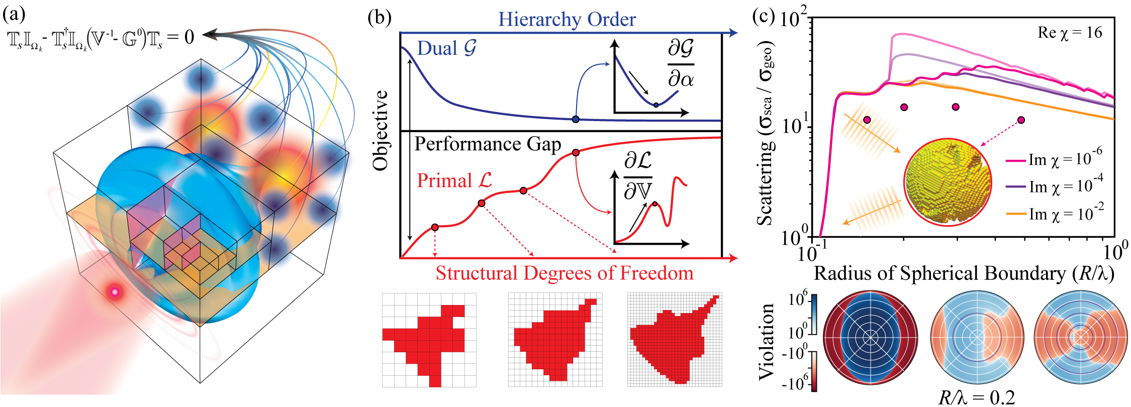
Figure 1: Schematic mean-field hierarchical bounds and application to scattering cross sections. (a) Like Maxwell’s equations, the definition of the $\mathbb{T}$ operator, (1), implicitly contains relations that must be obeyed at every spatial point. Present approaches to electromagnetic limits, however, only impose that this equality be satisfied on average, allowing bound solutions to exhibit highly unphysical local features. (b) By enforcing that the definition of the $\mathbb{T}$ operator be respected on successively smaller subdomains or clusters, described by constraints $\alpha$, the dual bound objective $\mathcal{G}$ given in (6) acquires a hierarchical structure that mirrors the primal problem of optimizing some objective $\mathcal{L}$ in (4), in terms of an increasing number of structural degrees of freedom contained in the scattering potential $\mathbb{V}$. In the limit of point clusters and complete structural freedom, the two problem statements are equivalent; see discussion in main text. (c) Upper bounds on the plane-wave scattering cross-section $\sigma_{\text{sca}}$, relative to the geometric cross section of the domain $\sigma_{\text{geo}}$, for any structure bounded by a sphere of radius $R$. Lighter lines result by enforcing that power be conserved globally, as in Refs. Molesky et al. (2020a); Gustafsson et al. (2020). Similarly colored dark lines result when analogous equalities are asserted over eight, evenly spaced, radial subdomains. A profile of one of the density-optimized structures is shown as an inset. Shown below are logarithmic color maps of the corresponding violation in the real part of (2) for one, two and four (evenly spaced) shell clusters, in the plane perpendicular to both the incoming wave vector and direction of polarization.

In this Letter, we remedy this issue, and euclidate fundamental connections between dual bounds and structural optimization, by proposing the adoption of constraint hierarchies originating from the central equality of scattering theory—the definition of the $\mathbb{T}$ operator. The approach functions, in essence, as a collection of successively refined mean-field theories Opper and Saad (2001). At the base of the hierarchy, only the global (spatially integrated) real and reactive power constraints studied in Refs. Molesky et al. (2020a); Gustafsson et al. (2020) are imposed on the optimization objective, equating these prior results to a first-order mean-field approximation. In every subsequent refinement, the computational domain is decomposed (partitioned) into increasingly small, nested, subdomains, which, through projection, induces additional scattering constraints and results in a higher-order approximation, Fig. 1. Reminiscent of multi-grid and multi-scale methods Chen and Liu (2012); Zhu and Cangellaris (2006), the order of the hierarchy thus acts as a resolution “knob” for systematically controlling the extent to which Maxwell’s equations are respected locally, allowing multiple length scales (beyond the size of the domain) to be considered concurrently. Correspondingly, the method also presents a complementary top-down approach to inverse design: the solution of any optimization problem in the constraint hierarchy is always “more optimal” than what is conceptually possible if full wave physics are completely obeyed, whereas inverse design in a finite number of structural degrees of freedom is always suboptimal; in the limit of point subdomains (infinite mean-field order) and infinitesimal structural variations (vanishing “voxels”) the two views agree, and, if strong duality holds Boyd and Vandenberghe (2004), the bounds solution in fact determines a globally optimal structure. More concretely, proof-of-concept application of the method to the problem of enhancing radiative emission from a dipolar current source in the near field of a structured medium, crucial to optical sensing and quantum information technologies Raussendorf and Briegel (2001); Belushkin et al. (2018); Chakravarthi et al. (2020), yields bounds that come substantially closer to the values found by density optimization.

Notation—Throughout, $\mathbb{I}$ is used to denote the identity operator, and subscripts on operators (blackboard bold letters) are used as a booking device for the domains and codomains of definition. When only a single subscript is shown, the domain and codomain are identical. The subscripts $b$ and $s$ mark spatial locations as part of either the background ($b$) or scattering object ($s$) within in some predefined domain, $\Omega$. When an operator appears without subscripts, its domain and codomain are $\Omega$. $\mathbb{G}^{\text{0}}$ refers to the background Green’s function Molesky et al. (2020a), and hence depends on $\Omega$. $\mathbb{V}$ is used to denote the scattering potential, i.e. any polarizable medium not included in $\mathbb{G}^{\text{0}}$.

Constraints—In scattering theory Tsang et al. (2004); Molesky et al. (2020b), the role commonly played by wave equations (e.g. Maxwell’s equations) is typified by the $\mathbb{T}$ operator, defined as

$$\mathbb{I}_{s}=\mathbb{I}_{s}\left(\mathbb{V}^{-1}-\mathbb{G}^{\text{0}}\right)\mathbb{T}_{s};$$ (1)

which, together with knowledge of $\mathbb{G}^{\text{0}}$ and $\mathbb{V}$, abstractly determines all fields for a given source. This operational picture lies at the heart of the hierarchical construction. Any number of manifestly true relations can be generated by probing (1) with linearly independent combinations of fields from the right and linear functionals from the left, and, by Lagrange duality, any set of constraints can be used to produce calculable bounds on any given optimization objective (so long as the dual remains soluble) Boyd and Vandenberghe (2004). Therefore, because every relation derived from (1) is physical, each and every such collection of equalities generates some physical bound on any wave process.

As may be expected, certain choices are more naturally motivated than others, and the difficulty of the associated convex optimization problem that must be solved in each case depends closely on the particular constraints chosen. If all identities contained in (1) are imposed over some complete basis, then the associated primal problem is equivalent to completely free structural optimization, and in computing a solution to the dual (convex) system an actual $\mathbb{T}$ operator must be nearly constructed. (The collection of all input–output relationships determines any operator, and so, the only caveat that makes this statement inexact is that the solution of the dual problem may not satisfy every constraint.) Hence, making full use of (1) likely results in an optimization problem comparable to bottom-up structural inverse design Lazarov et al. (2016); Jin et al. (2020). On the other hand, if only a select subset of the information contained in (1) is kept, the simplicity of determining bounds can be greatly reduced, at the cost of allowing the discovered solution to inevitably violate some local scattering relation(s). But, unlike standard calculations where the implications of some “partially valid” model on actual solutions are seldom known a priori, solving a dual problem always determines a bound on performance, and therefore always yields useful information.

To begin, it is simplest to work with (1) using either the image or polarization field resulting from the action of $\mathbb{T}_{s}$ on a single source field $\left|\textbf{S}\right>$, $\mathbb{T}_{s}\left|\textbf{S}\right>\mapsto\left|\textbf{T}\right>$ Molesky et al. (2020a), or, with this image and the action of $\mathbb{I}_{s}$ on $\left|\textbf{S}\right>$, $\left\{\mathbb{T}_{s}\left|\textbf{S}\right>\mapsto\left|\textbf{T}\right>,~{}\mathbb{I}_{s}\left|\textbf{S}\right>\mapsto\left|\textbf{R}\right>\right\}$ . Letting $\mathcal{R}=\left\{\Omega_{k}\right\}_{{}_{K}}$ denote the sets of chosen subdomains, the first choice leads to cluster constraints of the form

$$\left(\forall\Omega_{k}\in\mathcal{R}\right)~{}\left<\textbf{S}\right|\mathbb{I}_{{}_{\Omega_{k}}}\left|\textbf{T}\right>=\left<\textbf{T}\right|\mathbb{U}\mathbb{I}_{{}_{\Omega_{k}}}\left|\textbf{T}\right>,$$ (2)

where $\mathbb{U}=\mathbb{V}^{-1\dagger}-\mathbb{G}^{\text{0}\dagger}$ so that $\operatorname{Asym}\left[\mathbb{U}\right]$ is positive definite, and $\langle\textbf{F}|\textbf{G}\rangle=\int d^{3}\textbf{x}\,\textbf{F}(\textbf{x})^{*}\cdot\textbf{G}(\textbf{x})$ is a complex-conjugate inner product (spatial integration over the entire domain). The second choice allows for greater variety, and, $\left(\forall\Omega_{k}\in\mathcal{R}\right)$, any combination of

$$\left<\textbf{S}\right|\mathbb{I}_{{}_{\Omega_{k}}}\left|\textbf{R}\right>=\left<\textbf{R}\right|\mathbb{I}_{{}_{\Omega_{k}}}\left|\textbf{R}\right>, \left<\textbf{S}\right|\mathbb{I}_{{}_{\Omega_{k}}}\left|\textbf{T}\right> =\left<\textbf{R}\right|\mathbb{I}_{{}_{\Omega_{k}}}\left|\textbf{T}\right>,$$

$$\left<\textbf{S}\right|\mathbb{I}_{{}_{\Omega_{k}}}\left|\textbf{R}\right>=\left<\textbf{T}\right|\mathbb{U}\mathbb{I}_{{}_{\Omega_{k}}}\left|\textbf{R}\right>,$$ (3)

appear to be, at least presently, sensible.

Both (2) and (3) follow from (1) based on the properties of $\mathbb{I}_{s}$, $\mathbb{T}_{s}$, and the commutativity of spatial projection. $\left(\forall~{}U,~{}V\subset\mathbb{R}^{n}\right)~{}U\cap V=V\cap U$, and so, as $\mathbb{I}_{s}$ and $\mathbb{I}_{{}_{\Omega_{j}}}$ both denote projections into spatial locations, $\mathbb{I}_{{}_{\Omega_{j}}}\mathbb{I}_{s}=\mathbb{I}_{s\cap_{\Omega_{j}}}=\mathbb{I}_{s}\mathbb{I}_{{}_{\Omega_{j}}}$, implying that (for any $\Omega_{j}\subset\Omega$) $\mathbb{I}_{s}\mathbb{I}_{{}_{\Omega_{j}}}=\mathbb{I}_{s}^{2}\mathbb{I}_{{}_{\Omega_{j}}}=\mathbb{I}_{s}\mathbb{I}_{{}_{\Omega_{j}}}\mathbb{I}_{s}$, $\mathbb{I}_{{}_{\Omega_{j}}}\mathbb{T}_{s}=\mathbb{I}_{{}_{\Omega_{j}}}\mathbb{I}_{s}\mathbb{T}_{s}=\mathbb{I}_{s}\mathbb{I}_{{}_{\Omega_{j}}}\mathbb{T}_{s}$, and $\mathbb{I}_{{}_{\Omega_{j}}}\mathbb{I}_{s}=\mathbb{I}_{{}_{\Omega_{j}}}\mathbb{T}_{s}^{\dagger}\mathbb{U}\mathbb{I}_{s}=\mathbb{T}_{s}^{\dagger}\mathbb{U}\mathbb{I}_{{}_{\Omega_{j}}}\mathbb{I}_{s}$. If only a single cluster corresponding to the entire domain $\Omega$ is used, then (2) reduces to the constraints examined in Ref. Molesky et al. (2020a), with the symmetric (Hermitian) and anti-symmetric (skew-Hermitian) parts of (2), $\operatorname{Im}\left[\left<\textbf{S}|\textbf{T}\right>\right]=\left<\textbf{T}\right|\operatorname{Asym}\left[\mathbb{U}\right]\left|\textbf{T}\right>$ and $\operatorname{Re}\left[\left<\textbf{S}|\textbf{T}\right>\right]=\left<\textbf{T}\right|\operatorname{Sym}\left[\mathbb{U}\right]\left|\textbf{T}\right>,$ representing the global (averaged over the entire scatterer) conservation of real and reactive power, respectively.

Every equality of the form given by (2) represents a similar requirement on how power may be transferred between an exciting field and the response (polarization) current it generates. As verified in Fig. 2, these additions are crucial for properly describing near-field interactions. When no constraints other than the global conservation of real and reactive power are imposed, the optimal $\left|\textbf{T}\right>$ discovered via the method presented in Refs. Molesky et al. (2020a); Gustafsson et al. (2020) conserves power only by canceling equally large positive and negative violations over $\Omega$, Fig. 1: locally, the power drawn from the incident field is either far greater, or far smaller, than what can be accounted for by absorption and scattering. By successively subdividing the domain, the scale over which such cancellations of unphysical behavior can occur is continually reduced, and because there is always an implicit interaction length scale in $\mathbb{U}$ set by material loss and the background Green’s function, these tighter requirements ultimately lead to increasingly physical fields. Intuitively, beyond a certain critical size, the effect produced by rapid spatial variations of violation is no different than an averaged “mean” field which respects the constraints at all spatial points.

Though notionally similar, the role of (1) in (3) (third line) requires a distinct interpretation. Rather than describing how power may be transferred between the source and the polarization field it generates within subregions of the domain, these relations state that within the scatterer $\mathbb{U}^{\dagger}$ must effectively “invert” $\left|\textbf{T}\right>$, reproducing the projection of the source into the scattering object, $\left|\textbf{R}\right>$. If (3) were true pointwise, instead of on average over some finite collection of subsets, then both $\left|\textbf{R}\right>$ and $\left|\textbf{T}\right>$ would be produced by a geometry with scattering material at all locations x where $\textbf{R}(\textbf{x})=\textbf{S}(\textbf{x})$, equating this limit with structural inverse design.

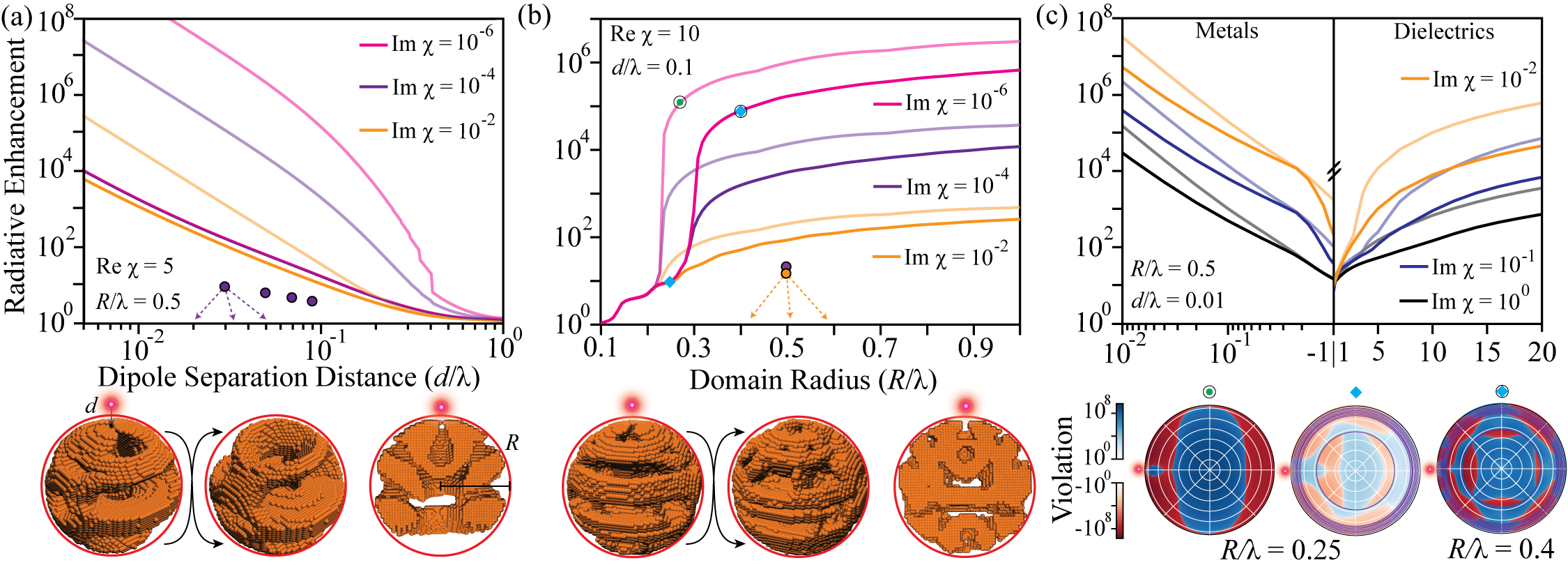
Figure 2: Application to radiative Purcell enhancement. Following the same conventions as Fig. 1(c), for a dipolar source, proof-of-concept radial shell cluster constraint hierarchies are found to substantially alter both the conditions under which resonant (loss dependent) radiative emission enhancement can possibly occur, panels (a) and (b), and generally reduce the dependence of calculated limits on material properties, all panels. Throughout, the solid lines are calculated with $r_{\text{shell}}/R=\left\{0.97,0.95,0.93,0.91,0.89,0.87,0.85,0.6\right\}$. Key features are described in the main text. Profiles and cross cuts of two representative density optimized structures are displayed below (a) and (b). The color maps below (c) show spatial violations in the real part of (2) for the parameter values marked in (b). No notable Purcell enhancement is observed for $-1<\text{Re}\left[\chi\right]<1$.

Hierarchy—Through (2) and (3), any set of regions in $\Omega$ defines a collection of constraints on any observable property of the associated scattering theory; and in turn, these constraints define an optimization problem that bounds the observable, along with a dual solution $\left|\textbf{T}_{d}\right>$ or $\left\{\left|\textbf{T}_{d}\right>,~{}\left|\textbf{R}_{d}\right>\right\}$. Consider the collection $\mathcal{C}$ of all such sets of regions, $\mathcal{R}=\left\{\Omega_{k}\right\}_{K}$, with the properties that $\bigcup_{K}\Omega_{k}=\Omega$ and $\left(\forall k\neq j\right)~{}\Omega_{k}\cap\Omega_{j}=\emptyset$. Call $\mathcal{R}^{\prime}$ a refinement of $\mathcal{R}$, $\mathcal{R}^{\prime}\geq\mathcal{R}$, if $\left(\forall\Omega_{k}\in\mathcal{R}\right)~{}\exists\left\{\Omega_{j}\right\}_{J}\subset\mathcal{R}^{\prime}\ni\Omega_{k}=\bigcup_{j\in J}\Omega_{j}$, giving $\mathcal{C}$ a partial ordering. Directly, the map between collections of spatial sets and bounds on a given observable described above, restricted to $\mathcal{C}$, is monotonic. If $\mathcal{R}^{\prime}\geq\mathcal{R}$ then the associated bound for $\mathcal{R}^{\prime}$ is necessarily tighter (bigger or smaller depending on the objective) than the bound for $\mathcal{R}$. Every refinement $\mathcal{R}^{\prime}\geq\mathcal{R}$ in $\mathcal{C}$ results in a split of multipliers of the optimization Lagrangian, as each constraint is decomposed into a set of constraints over the matching subregions. Therefore, the codomain of the dual function corresponding to $\mathcal{R}^{\prime}$ contains the codomain of the dual function corresponding to $\mathcal{R}$, and so the minima (resp. maxima) of the dual functions maintains the ordering of $\mathcal{C}$, leading to a monotonically tighter bounds, Fig. 1. Hence, successive division of the spatial regions used in generating constraints via (1) indeed yields a well defined hierarchy of $\mathbb{T}$ operator bounds, approximating any optimization problem with increasingly better accuracy. Moreover, less refined solutions are always dual feasible points for more refined optimizations, and by evaluating the pointwise versions of (2) and (3) that would hold under complete compliance with the scattering theory for any given dual solution $\left|\textbf{T}_{d}\right>$ (resp. $\left\{\left|\textbf{T}_{d}\right>,~{}\left|\textbf{R}_{d}\right>\right\}$), as in the heat maps of Fig. 1 and Fig. 2, it is possible to assess where inconsistency is occurring, and use this knowledge to inform further regional decompositions.

The hierarchy construction amounts, conceptually, to a set of successively expanded mean-field theories Soukoulis and Levin (1977); Plefka (1982); Jin et al. (2016). Traditionally, one of the standard ways in which a mean-field theory is constructed is to consider the question of minimizing the Gibb’s free energy of a system over the collection of all possible statistical distributions, parameterized by constraints on its moments (expectation values, two-point correlations, etc). To make such problems tractable, the form of the distribution is simplified in some way (e.g. partitioning the true system into effectively interacting spatial clusters) before carrying out a local optimization on the resulting (generally nonconvex) problem. The solution, stationary and self-consistent with respect to the moments, is called a mean field since to lowest order it describes each component of the system as interacting with one other “averaged” body. By switching to a scattering description, the need for simplification is shifted from the objective to the constraints, but the interpretation of the solution is virtually unaltered. In either case, it is a field that is self-consistent when variations around average values are neglected.

Bounds—Generalizing the program given in Ref. Molesky et al. (2020a), in any order of the hierarchy, the calculation of bounds for any net power transfer (scattering) objective can be equated with a domain monotonic optimization problem described by a sesquilinear Lagrangian. Grouping the source terms for the constraints and objective, $\left|\textbf{S}\right>$ and $\left|\textbf{Q}\right>$, together as the super source $\left|\underline{\textbf{S}}\right>$

$$\mathcal{L}\left(\left\{\alpha_{k}^{\left(1\right)}\right\},\left\{\alpha_{k}^{\left(2\right)}\right\},\left|\textbf{T}\right>\right)=\begin{bmatrix}\left<\textbf{T}\right|&\left<\underline{\textbf{S}}\right|\end{bmatrix}\begin{bmatrix}\mathbb{Z}^{{}_{TT}}&\mathbb{Z}^{{}_{T\underline{S}}}\\ \mathbb{Z}^{{}_{\underline{S}T}}&\textbf{0}\end{bmatrix}\begin{bmatrix}\left|\textbf{T}\right>\\ \left|\underline{\textbf{S}}\right>\end{bmatrix};$$ (4)

where, supposing an objective of the form $\operatorname{Im}\left[\left<\textbf{Q}|\textbf{T}\right>\right]-\left<\textbf{T}\right|\mathbb{O}\left|\textbf{T}\right>$ Molesky et al. (2020a), the $\mathbb{Z}^{{}_{-,-}}$ operators are the linear couplings (depending on the multipliers) between the various fields

$$-\mathbb{Z}^{{}_{TT}} =\mathbb{O}+\sum_{k\in K}\alpha_{k}^{\left(1\right)}\operatorname{Sym}\left[\mathbb{U}\mathbb{I}_{{}_{\Omega_{k}}}\right]+\alpha_{k}^{\left(2\right)}\operatorname{Asym}\left[\mathbb{U}\mathbb{I}_{{}_{\Omega_{k}}}\right]$$

$$=\mathbb{O}+\operatorname{Sym}\left[\mathbb{U}\mathbb{R}^{\left(1\right)}\right]+\operatorname{Asym}\left[\mathbb{U}\mathbb{R}^{\left(2\right)}\right],$$

$$\mathbb{Z}^{{}_{TS}} =\mathbb{Z}^{{}_{ST}*}=\sum_{k\in K}\frac{\alpha_{k}^{\left(1\right)}}{2}\mathbb{I}_{{}_{\Omega_{k}}}+\frac{i\alpha_{k}^{\left(2\right)}}{2}\mathbb{I}_{{}_{\Omega_{k}}}=\frac{\mathbb{R}^{\left(1\right)}}{2}+\frac{i\mathbb{R}^{\left(2\right)}}{2},$$

$$\mathbb{Z}^{{}_{TQ}} =\mathbb{Z}^{{}_{QT}*}=\frac{i}{2}\mathbb{I},$$ (5)

$\mathbb{R}^{\left(1\right)}=\sum_{k\in K}\alpha_{k}^{\left(1\right)}\mathbb{I}_{{}_{\Omega_{k}}}$, $\mathbb{R}^{\left(2\right)}=\sum_{k\in K}\alpha_{k}^{\left(2\right)}\mathbb{I}_{{}_{\Omega_{k}}}$, and $\left\{\alpha^{\left(1\right)}_{k}\right\}$ and $\left\{\alpha^{\left(2\right)}_{k}\right\}$ are the sets of Lagrange multipliers for all symmetric and anti-symmetric constrains respectively. For both scattering and radiative Purcell enhancement, $\mathbb{O}=\operatorname{Asym}\left[\mathbb{V}^{-1\dagger}\right]$; see Ref. Molesky et al. (2020a) for further details. Because optimization is always formulated in terms of real numbers, the total $\mathbb{Z}$ matrix is Hermitian.

The unique stationary point of $\eqref{Lgen}$ with respect to variations in $\left|\textbf{T}\right>$ occurs when $\left|\textbf{T}\right>=\mathbb{Z}^{{}_{TT}-1}\mathbb{Z}^{{}_{T\underline{S}}}\left|\underline{\textbf{S}}\right>=\mathbb{Z}^{{}_{TT}-1}\left(\mathbb{Z}^{{}_{TS}}\left|\textbf{S}\right>+\mathbb{Z}^{{}_{TQ}}\left|\textbf{Q}\right>\right),$ and so the dual of (4), $\mathcal{G}=\text{max}_{\mathcal{F}}~{}\mathcal{L}$ where the domain $\mathcal{F}$ is set by the criterion that $\text{max}~{}\mathcal{L}$ is finite, is

$$\mathcal{G}=-\left<\underline{\textbf{S}}\right|\mathbb{Z}^{{}_{\underline{S}T}}\mathbb{Z}^{{}_{TT-1}}\mathbb{Z}^{{}_{T\underline{S}}}\left|\underline{\textbf{S}}\right>.$$ (6)

Note that a set $\left\{\left<\alpha^{\left(1\right)}_{k},\alpha^{\left(2\right)}_{k}\right>\right\}$ lies within $\mathcal{F}$ so long as $\mathbb{Z}^{{}_{TT}-1}$ is positive definite Strang (2007).

Because the dual problem is convex and gradients of the dual reproduce the constraints set by (2), if a stationary point within the feasibility region is found, then strong duality holds and the maximum of the objective is $\operatorname{Im}\left[\left<\textbf{Q}|\textbf{T}\right>\right]-\left<\textbf{T}\right|\mathbb{O}\left|\textbf{T}\right>$, with $\left|\textbf{T}\right>$ determined as above using the multiplier values set by the simultaneous zero point of the gradients (constraints). If no such point exists in $\mathcal{F}$, then the unique minimum value of $\mathcal{G}$ attained on the boundary, caused by $\mathbb{Z}^{{}_{TT}}$ becoming semi-definite, remains a bound on the optimization problem.

Example—As an initial exploration of $\mathbb{T}$ operator constraint hierarchies, under (2), Fig. 2 illustrates how the introduction of spherically symmetric (concentric) shell clusters alters bounds on Purcell enhancement (radiative emission from a dipolar current source in the vicinity of a structured medium normalized to emission in vacuum) compared to past global-conservation arguments Molesky et al. (2020a); Gustafsson et al. (2020). Even with a choice of relatively simple clusters, which leads to considerable numerical simplifications, but also limit the extent to which violation can be localized, two promising trends are observed. First, the number of material and domain size combinations displaying resonant response characteristics, as qualified by a roughly inverse scaling between radiative enhancement and material loss $\text{Im}\left[\chi\right]$, is reduced. To the best of our knowledge, no compact single dielectric material device design exhibits such behavior for values of $\text{Im}\left[\chi\right]$ comparable to those considered here, leading to potentially gigantic gaps between calculated limits and the findings of density optimization, Fig. 2 (a). So long as strong duality is present, which holds for all of (a) and (b) below $R/\lambda\approx 0.3$, the dependence of the cluster bounds on $\text{Im}\left[\chi\right]$ is greatly suppressed; and when a relation between these quantities is observed for $\text{Im}\left[\chi\right]\lesssim 10^{-2}$, the corresponding optimal polarization field, $\left|\textbf{T}\right>$, implies large local constraint violations, as shown by the spatial color maps of the real part of (2) included below Fig. 2 (c). Similarly, Fig. 2 (b) and (c), for separations as small as $d/\lambda=10^{-2}$ and domains as large as $R/\lambda=1$, cluster-bound values are substantially smaller (often an order of magnitude or more) for strong metallic and dielectric materials, $|\text{Re}\left[\chi\right]|\gg 5$. Nevertheless, the limits remain several orders of magnitude larger than what is observed in devices discovered by density optimization when such values of $\chi$ are supposed, suggesting further room for improvement.

This work was supported by the National Science Foundation under Grants No. DMR 1454836, DMR 1420541, DGE 1148900, EFMA 1640986, the Cornell Center for Materials Research MRSEC (award no. DMR1719875), and the Defense Advanced Research Projects Agency (DARPA) under Agreement No. HR00112090011. The views, opinions and/or findings expressed herein are those of the authors and should not be interpreted as representing the official views or policies of any institution. The authors thank Cristian L. Cortes for useful discussion.

References

- Jensen and Sigmund (2011) J. S. Jensen and O. Sigmund, Laser & Photonics Reviews 5, 308 (2011).
- Molesky et al. (2018) S. Molesky, Z. Lin, A. Y. Piggott, W. Jin, J. Vučković, and A. W. Rodriguez, Nature Photonics 12, 659 (2018).
- Men et al. (2014) H. Men, K. Y. Lee, R. M. Freund, J. Peraire, and S. G. Johnson, Optics express 22, 22632 (2014).
- Meng et al. (2018) F. Meng, B. Jia, and X. Huang, Advanced Theory and Simulations 1, 1800122 (2018).
- Chen et al. (2019) Y. Chen, F. Meng, B. Jia, G. Li, and X. Huang, Physica Status Solidi (RRL)–Rapid Research Letters 13, 1900175 (2019).
- Okoro et al. (2017) C. Okoro, H. E. Kondakci, A. F. Abouraddy, and K. C. Toussaint, Optica 4, 1052 (2017).
- Callewaert et al. (2018) F. Callewaert, V. Velev, P. Kumar, A. Sahakian, and K. Aydin, Scientific Reports 8, 1358 (2018).
- Meem et al. (2020) M. Meem, S. Banerji, C. Pies, T. Oberbiermann, A. Majumder, B. Sensale-Rodriguez, and R. Menon, Optica 7, 252 (2020).
- Chung and Miller (2020) H. Chung and O. D. Miller, Optics Express 28, 6945 (2020).
- Lin et al. (2020) Z. Lin, C. Roques-Carmes, R. Pestourie, M. Soljačić, A. Majumdar, and S. G. Johnson, arXiv:2006.09145 (2020).
- Lin et al. (2016) Z. Lin, A. Pick, M. Lončar, and A. W. Rodriguez, Physical Review Letters 117, 107402 (2016).
- Long et al. (2019) Y. Long, J. Ren, Y. Li, and H. Chen, Applied Physics Letters 114, 181105 (2019).
- Christiansen et al. (2019) R. E. Christiansen, F. Wang, and O. Sigmund, Physical Review Letters 122, 234502 (2019).
- Gill et al. (2019) P. E. Gill, W. Murray, and M. H. Wright, Practical optimization (SIAM, 2019).
- Angeris et al. (2019) G. Angeris, J. Vučković, and S. P. Boyd, ACS Photonics 6, 1232 (2019).
- Molesky et al. (2020a) S. Molesky, P. Chao, W. Jin, and A. W. Rodriguez, Physical Review Research 2, 033172 (2020a).
- Gustafsson et al. (2020) M. Gustafsson, K. Schab, L. Jelinek, and M. Capek, New Journal of Physics (2020).
- Kuang et al. (2020) Z. Kuang, L. Zhang, and O. D. Miller, arXiv:2002.00521 (2020).
- Trivedi et al. (2020) R. Trivedi, G. Angeris, L. Su, S. Boyd, S. Fan, and J. Vuckovic, arXiv:2003.00374 (2020).
- Jackson (1999) J. D. Jackson, Classical electrodynamics (AAPT, 1999).
- Opper and Saad (2001) M. Opper and D. Saad, Advanced mean field methods: Theory and practice (MIT press, 2001).
- Chen and Liu (2012) J. Chen and Q. H. Liu, Proceedings of the IEEE 101, 242 (2012).
- Zhu and Cangellaris (2006) Y. Zhu and A. C. Cangellaris, Multigrid finite element methods for electromagnetic field modeling, Vol. 28 (John Wiley & Sons, 2006).
- Boyd and Vandenberghe (2004) S. Boyd and L. Vandenberghe, Convex Optimization (Cambridge university press, 2004).
- Raussendorf and Briegel (2001) R. Raussendorf and H. J. Briegel, Physical Review Letters 86, 5188 (2001).
- Belushkin et al. (2018) A. Belushkin, F. Yesilkoy, and H. Altug, ACS Nano 12, 4453 (2018).
- Chakravarthi et al. (2020) S. Chakravarthi, P. Chao, C. Pederson, S. Molesky, K. Hestroffer, F. Hatami, A. W. Rodriguez, and K.-M. C. Fu, arXiv:2007.12344 (2020).
- Tsang et al. (2004) L. Tsang, J. A. Kong, and K.-H. Ding, Scattering of electromagnetic waves: theories and applications, Vol. 27 (John Wiley & Sons, 2004).
- Molesky et al. (2020b) S. Molesky, P. S. Venkataram, W. Jin, and A. W. Rodriguez, Physical Review B 101, 035408 (2020b).
- Lazarov et al. (2016) B. S. Lazarov, F. Wang, and O. Sigmund, Archive of Applied Mechanics 86, 189 (2016).
- Jin et al. (2020) W. Jin, W. Li, M. Orenstein, and S. Fan, arXiv:2005.04840 (2020).
- Note (1) Additional sources and fields, not necessarily related to the problem, may also be included to more completely explore , and push the resulting primal optimization problem towards structural inverse design.
- Soukoulis and Levin (1977) C. Soukoulis and K. Levin, Physical Review Letters 39, 581 (1977).
- Plefka (1982) T. Plefka, Journal of Physics A 15, 1971 (1982).
- Jin et al. (2016) J. Jin, A. Biella, O. Viyuela, L. Mazza, J. Keeling, R. Fazio, and D. Rossini, Physical Review X 6, 031011 (2016).
- Strang (2007) G. Strang, Computational science and engineering (Wellesley-Cambridge Press, 2007).