Complementary Language Model and Parallel Bi-LRNN for False Trigger Mitigation

Abstract

False triggers in voice assistants are unintended invocations of the assistant, which not only degrade the user experience but may also compromise privacy. False trigger mitigation (FTM) is a process to detect the false trigger events and respond appropriately to the user. In this paper, we propose a novel solution to the FTM problem by introducing a parallel ASR decoding process with a special language model trained from “out-of-domain” data sources. Such language model is complementary to the existing language model optimized for the assistant task. A bidirectional lattice RNN (Bi-LRNN) classifier trained from the lattices generated by the complementary language model shows a $38.34\%$ relative reduction of the false trigger (FT) rate at the fixed rate of $0.4\%$ false suppression (FS) of correct invocations, compared to the current Bi-LRNN model. In addition, we propose to train a parallel Bi-LRNN model based on the decoding lattices from both language models, and examine various ways of implementation. The resulting model leads to further reduction in the false trigger rate by $10.8\%$.

Index Terms: Voice Trigger Detection, False Trigger Mitigation, Lattice RNN, Language Model

1 Introduction

Voice trigger detection is a vital part of current voice assistant products. In such systems, one or multiple trigger phrases are defined for users to invoke the device to process voice requests. The design of a trigger detector is often constrained by limited computation resources and power consumption of hardware, therefore we often adopt simple DSP and acoustic models [1, 2]. In practice, a trigger detector is usually operated in a low-false-rejection mode in order to allow most acoustic samples to be passed to downstream processes. However, such design may cause the assistant (wrongly) respond to unintended acoustic inputs. There are also cases when users accidentally invoke the assistant through a UI element such as a button-press or a particular gesture. Such unintended invocations of voice assistants can be referred to as “false triggers”. To mitigate the false trigger cases, one can introduce an extra process to determine whether an acoustic sample is intended or not, which is in essence a binary classification problem.

The false trigger mitigation process can make use of both acoustic and linguistic clues from the input sample. When the errors are due to voice trigger detector, an intuitive approach is to feed the acoustic sample into an ASR system and check for the existence of trigger phrases in the 1-best output [3]. In more general cases, the text output contains the intent information from the user, therefore can be used as input to the classifier. In [4], the 1-best output is encoded as an LSTM embedding to represent the linguistic feature. It is combined with the LSTM embedding of the acoustic features, and decoder features including trellis entropy, Viterbi cost, confidence and average number of arcs as the final input feature set to the classier. Considering the ASR results may contain errors, the decoder features are designed explicitly to capture the ambiguity during the decoding process. A recent follow-up work [5] focuses on improving the acoustic features by incorporating utterance-level representations. It also introduces dialog-type information to facilitate the classifier to make better decisions.

To build an intent classifier, the authors of [6] propose a condense representation of lattices from ASR decoder, called “Lattice RNN” (LRNN). By introducing a pooling operation over the incoming arcs of each node in the lattice, and a propagation operation over the outgoing arcs of the nodes, the authors are able to construct a neural network on a lattice, and encode the whole lattice information as the vector output from the final node of the lattice. The LRNN embedding is used as the input vector of the intent classifier, which achieves better accuracy and faster run-time, compared to the baseline model running on N-best results. A similar approach can be applied to the FTM task. Our previous work [7] redefined the feature set attached to each arc in the decoder lattice, and extended the network to bi-directional (Bi-LRNN). The decoding lattice is encoded as the concatenation of hidden layers from the start and end nodes of the lattice. Thus a classifier built on top of the Bi-LRNN is able to mitigate the false trigger cases significantly. A recent work [8] explored the use of graph neural networks (GNN) to encode the decoding lattice, which achieves similar accuracy as the Bi-LRNN representation with more efficient training.

In this paper, we investigate the impact of the decoder’s language model (LM) on false trigger mitigation. Considering that the voice assistant’s LM is usually well trained with in-domain data, and the LM also tends to see more usage data with the trigger phrase at the beginning, it is likely that the LM is biased towards the in-domain data, which thereby biases it towards detecting the trigger phase. This bias may reduce the power of the decoding lattice in mitigating false triggers. In our study, we train a new LM that is not biased to the trigger phrase and in-domain data. We compare the mitigation performance between the Bi-LRNN classifiers built from the the lattice outputs of different LMs. We further investigate how to make use of the complementary information in two different language models, and propose some approaches to build parallel Bi-LRNN, which leads to further improvement in false trigger mitigation.

2 Method

2.1 Bi-LRNN for false trigger mitigation

In our baseline Bi-LRNN system, we obtain the word hypothesis lattice $L$ for an acoustic sample $X$, from the ASR decoder. The lattice consists of a start node, an end node, and other intermediate nodes. The nodes are connected via arcs and each arc has a feature vector associated with it. The Bi-LRNN computes a forward and backward latent embedding for each node in the lattice (refer to [7] for more details).

The final outputs of the Bi-LRNN are the forward latent embedding of the end node $\textbf{h}_{f}(s_{end})$ and backward latent embedding of the start node $\textbf{h}_{b}(s_{start})$, where $s_{start}$ and $s_{end}$ denote the lattice’s start and end nodes. A feed-forward classifier then takes the input as $[\textbf{h}_{f}(s_{start}),\textbf{h}_{b}(s_{end})]$. The classifier gives a real valued output $y\in[0,1]$, which is converted to a label $l_{pred}\in\{0,1\}$ by choosing a threshold $t$. The threshold can be kept fixed at certain value, or can be evaluated empirically on the cross validation set, to achieve the desirable False Suppression (FS) of invocation rate.

2.2 Parallel decoding with complementary LMs

A typical ASR decoding process can be formulated as searching the best word sequence $W^{*}$ that maximizes (1), where $P\left(X\mid W\right)$ denotes acoustic model (AM), representing the conditional probability of acoustic features $X$ given a word sequence $W$, and $P\left(W\right)$ denotes language model (LM), representing the probability of any word sequence $W$. Ideally, the LM of an ASR system should approximate the distribution of all the word sequences that could reach the decoder. However, in practice, the voice assistant application is only designed to respond to a relevant set of user requests. So the LM is usually trained to maximize the likelihood of in-domain sentences. If we refer to the in-domain sentences as a class $\mathcal{L}_{D}$, and out-of-domain sentences as a class $\mathcal{L}_{O}$, the ASR LM trained from in-domain data can be explicitly represented as $P\left(W\mid\mathcal{L}_{D}\right)$ in (2), with $P\left(\mathcal{L}_{D}\right)$ denoting the prior probability of in-domain usage.

$$W^{*} =\arg\underset{W}{\max}\left\{P\left(X\mid W\right)P\left(W\right)\right\}$$ (1)

$$=\arg\underset{W}{\max}\left\{P\left(X\mid W,\mathcal{L}_{D}\right)P\left(W\mid\mathcal{L}_{D}\right)P\left(\mathcal{L}_{D}\right)\right\}$$ (2)

To use the ASR decoding information to determine whether a sequence of acoustic features represent an unintended invocation, we can compute the probability of in-domain usage given the acoustic observation, $P\left(\mathcal{L}_{D}\mid X\right)$. This measurement can be expanded as in (4), in which the first factor is the summation of AM and LM probabilities over all sentence hypotheses. An approximation can be made to apply the summation over the resulting lattice paths during decoding, when ignoring the low likelihood word sequences being pruned. The Bi-LRNN embedding can be interpreted as an implicit representation of such measurement with more flexibility and modeling capacity. [7]

$$P\left(\mathcal{L}_{D}\mid X\right) =P\left(X\mid\mathcal{L}_{D}\right)P\left(\mathcal{L}_{D}\right)/P\left(X\right)$$ (3)

$$= \frac{\sum_{i}\left\{P\left(X\mid W_{i},\mathcal{L}_{D}\right)P\left(W_{i}\mid\mathcal{L}_{D}\right)\right\}P\left(\mathcal{L}_{D}\right)}{P\left(X\right)}$$ (4)

The drawback of the above measurement in (4) is that $P\left(W\mid\mathcal{L}_{D}\right)$ only contains in-domain information, so its power of rejecting false triggered samples may be limited. If we have a good estimation of out-of-domain sentences with LM $P\left(W\mid\mathcal{L}_{O}\right)$, we can construct a complementary measurement, $P\left(\mathcal{L}_{O}\mid X\right)$, which in theory should have more power to reject false trigger. Equation (5) implies we will run ASR decoding with a different set of LM, $P\left(W\mid\mathcal{L}_{O}\right)$, to generate lattices different from the default ones. We can apply the similar Bi-LRNN operation on the out-of-domain lattices for more modeling capacity.

$$P\left(\mathcal{L}_{O}\mid X\right)=\frac{\sum_{i}\left\{P\left(X\mid W_{i},\mathcal{L}_{O}\right)P\left(W_{i}\mid\mathcal{L}_{O}\right)\right\}P\left(\mathcal{L}_{O}\right)}{P\left(X\right)}$$ (5)

Furthermore, we can derive a probability ratio measurement as shown in (6), which adopts the ratio between the in-domain and out-of-domain probabilities given the acoustic observation to balance the suppression/trigger decision. This measurement implies two ASR decoders can be run in parallel to achieve two different lattices from the same acoustic input. By combining the information from both lattices, we may be able to achieve better discriminative capacity between the two classes. Once more, this measurement can be generalized by training two Bi-LRNNs from the lattices of two decoders, and hopefully the network can learn more complex relationship between the two lattices when the targeting cost function is set to minimize the classification errors.

$$\frac{P\left(\mathcal{L}_{D}\mid X\right)}{P\left(\mathcal{L}_{O}\mid X\right)}=\frac{\sum_{i}\left\{P\left(X\mid W_{i},\mathcal{L}_{D}\right)P\left(W_{i}\mid\mathcal{L}_{D}\right)\right\}P\left(\mathcal{L}_{D}\right)}{\sum_{j}\left\{P\left(X\mid W_{j},\mathcal{L}_{O}\right)P\left(W_{j}\mid\mathcal{L}_{O}\right)\right\}P\left(\mathcal{L}_{O}\right)}$$ (6)

2.3 Ensembling parallel Bi-LRNNs

In the error analysis (Section 3.4), we show that the base model is more accurate for some examples, and the out-of-domain model is better on others, depending on the true label of the example. Thus, the language models likely represent complementary information, and a model comprised of both the LMs could out-perform the individual models based on either of the LMs. To achieve this, the outputs from the two Bi-LRNN models can be combined in different ways before passing to the classifier. We explore the following ensembling techniques, and compare the FT rates achieved by each of them in Section 3.5:

• Combine scores from the pre-trained Bi-LRNNs: We take the prediction scores $y_{1}$ and $y_{2}$ from the two Bi-LRNNs trained separately, and pass them to a shallow classifier. (Only classifier layers are trained).

• Combine the Bi-LRNN embeddings from the pre-trained Bi-LRNNs: We take the latent Bi-LRNN embeddings $\textbf{h}_{1_{f}},\textbf{h}_{1_{b}},\textbf{h}_{2_{f}},\textbf{h}_{2_{b}}$ from the pre-trained Bi-LRNNs, and pass them to a classifier (Here again, only the classifier is trained).

• Train the Bi-LRNNs in parallel, by back-propagating the classifier loss: The setting is the same as the previous case, but we back-propagate the classifier loss to both the Bi-LRNNs as well. Thus, the entire model is trained end-to-end (from scratch or by loading the weights of the trained Bi-LRNNs and fine-tuning them). The schematic of the model is shown in Figure 1.

• Mixture of Experts: Instead of concatenating the embeddings of the two Bi-LRNNs, we can pass their weighted sum to the classifier. A Mixture of Experts model [9], computes the relative importance of each “expert” (in this case, the two Bi-LRNNs are the “experts”), and weighs the outputs of the models by a parameter $\alpha$. The weight parameter $\alpha$ determines the reliability of each Bi-LRNN for an input sample, and we pass a weighted sum of the lattice embeddings to a classifier $\left(\left[\alpha\mathbf{h}_{1_{f}}+\left(1-\alpha\right)\mathbf{h}_{2_{f}},\alpha\mathbf{h}_{1_{b}}+\left(1-\alpha\right)\mathbf{h}_{2_{b}}\right]\right)$. The model is trained end-to-end. The schematic of the model is shown in Figure 2.

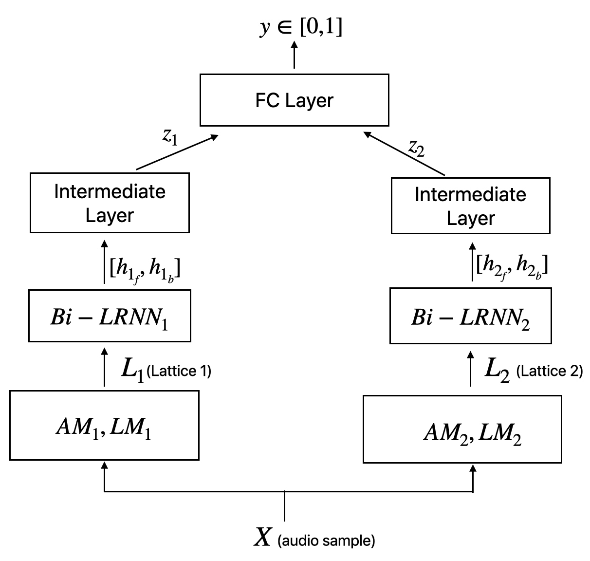
Figure 1: Schematic diagram of Parallel LRNN model

3 Experiment and results

3.1 FTM Dataset and evaluation metrics

All our experiments are performed on an FTM dataset [8], which is composed of far field usage samples with manual labels of “true trigger” (TT) and “false trigger” (FT) classes. The raw audio data are split into train, cv, dev, and eval sets for the purposes of training, cross-validation, development and evaluation. The train and cv sets are augmented by adding gain, noise, and speed perturbations, which increases the amount of training data by 3x. Table 1 summarizes the amount of data in each set and condition.

We train FTM classifiers for multiple epochs on the train set. The training epoch which achieved the lowest FT on the cv set is evaluated on the dev and eval sets. We expect our voice assistant to have minimal false triggers, and maximum true positives (minimal FS), for a good user-experience. We thus focus on the low FS regime in our DET curves, and the lower the AUC (Area Under Curve) of the DET curve, the better the model. In our experiments, we arbitrarily choose a small FS rate of $0.4\%$ to act as the operating point. So the False Trigger (FT) rate at this FS rate is the key metric in evaluating the false trigger mitigation models, while the AUC gives us an estimate of how good the model performs overall, irrespective of the operating point. We set the threshold that achieves the target FS rate (0.4%) on the dev set. The performance metric of concern to us is the corresponding FT rate on the eval set.

Label	train	cv	dev	eval
True Trigger	$14,225\times 3$	$1,582\times 3$	$5,829$	$11,646$
False Trigger	$6,223\times 3$	$691\times 3$	$5,657$	$11,316$

Table 1: FTM dataset for model training and evaluation

3.2 ASR decoder and baseline models

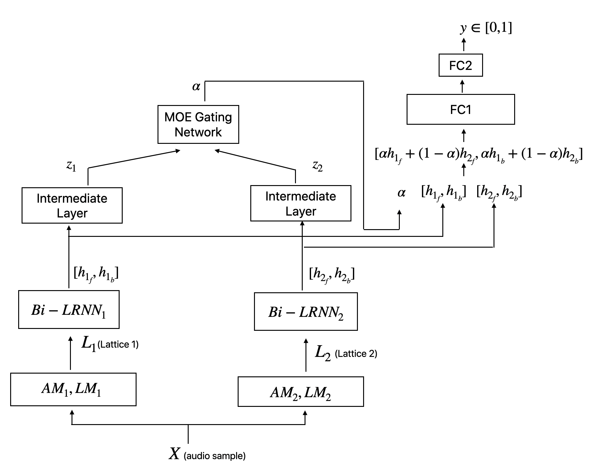
Figure 2: Schematic diagram of Mixture of Experts model

In all experiments, we adopt an internal ASR decoder with various model configurations. The acoustic model has an Hidden Markov model (HMM) and Convolutional Neural Network (CNN) hybrid structure [10], which is trained with filter bank features from US English speech data using cross-entropy and subsequent BMMI objective functions [11]. The CNN comprises 50 layers and uses the scaled exponential linear unit (SELU) activation function to achieve self-normalization during training [12], which achieves state-of-art performance. The baseline language model in the decoder is a 4-gram model interpolated from multiple sub-LMs trained from different data sources that are relevant to the far field application (in-domain). The data sources include enumerations of various usage domains, the re-decoding transcripts of live usage, and accumulated error corrections from the users. All the sub-LMs share a word lexicon with a vocabulary size of around $570K$. The final interpolated LM is pruned to contain about $4.9M$ 4-grams, $8.0M$ trigrams and $4.8M$ bigrams. We refer to this as the BaseLM.

3.3 Bi-LRNN based on complementary LM

In order to capture the out-of-domain usages, we consider the following data sources to train a complementary language model called ChatterLM. The first data source is from the automatic transcriptions of the dictation application; the second source is from the voice search application. The language usage styles of these two applications are different from that of the assistant application in our current study. The third source is artificial data generated from enumeration of extra use cases that are not relevant to the specific device under study. The ChatterLM is built in the same way as the BaseLM in production, then combined with the baseline AM for the ASR decoder to use.

With the two sets of ASR models, we generate decoding lattices on the FTM train and cv sets, then build two separate Bi-LRNN classifiers from the lattice features. To compare the accuracy between the two classifiers, we plot the DET curves of them on the eval sets in Figure 3 (We plot only the region of interest of the DET curve, ie $FS<1\%$). At the operation points around the fixed FS rate of $0.4\%$, the ChatterLM based classifier achieves a lower FT rate than the baseline classifier based on BaseLM. The relative reduction of FT rate is $38.34\%$ (FT reduces from $19.35\%$ for the BaseLM based Bi-LRNN to $11.93\%$ for the ChatterLM based Bi-LRNN). Such a significant FT rate reduction clearly indicates that the LM trained from out-of-domain data sources is more capable of detecting false triggers than the LMs trained from in-domain data sources.

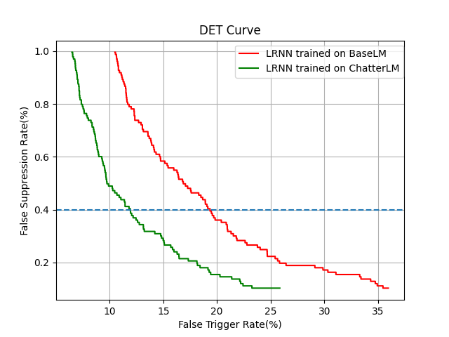
Figure 3: DET curves of BaseLM and ChatterLM LRNN models.

3.4 Error Analysis

We choose the two Bi-LRNN classifiers, which use lattices from the BaseLM and the ChatterLM respectively, to further analyze the error patterns. The idea is that if the models make mistakes on different samples, then ensembling them would provide complementary information, and thus improve the overall performance. We compute the matrix showing the number of samples for which the BaseLM Bi-LRNN and the ChatterLM Bi-LRNN got the predictions correct and incorrect (see Table 2). Both models achieve very high accuracy on the True Trigger (TT) class, with BaseLM being the more accurate of the two. For the False Trigger (FT) class, both models are less accurate, and ChatterLM is more accurate than BaseLM (only $3.66\%$ samples where BaseLM Bi-LRNN gets correct and ChatterLM Bi-LRNN gets wrong, cf. $20.27\%$ samples where BaseLM Bi-LRNN gets wrong and ChatterLM Bi-LRNN gets correct). These results align with our expectations, as the ChatterLM Bi-LRNN model is expected to be more accurate for unintended speech samples since it uses an LM trained on out-of-domain data, while the BaseLM Bi-LRNN uses the LM primarily trained on in-domain data. Thus, the models are stronger in different sample spaces, and should be able to complement each other when used together in an ensemble model.

		ChatterLM Correct	ChatterLM Wrong
TT	BaseLM Correct	$99.4\%$	$0.39\%$
	BaseLM Wrong	$0.08\%$	$0.09\%$
FT	BaseLM Correct	$66.3\%$	$3.66\%$
	BaseLM Wrong	$20.27\%$	$9.76\%$

Table 2: Error Analysis of True (TT) and False (FT) Triggers

3.5 Parallel Bi-LRNNs

Assuming we have two ASR models available, one comprising of the LM trained on in-domain data (BaseLM), and the other comprising of LM trained on out-of-domain data (ChatterLM), we can leverage the two complementary lattices by training parallel Bi-LRNN classifiers. We implement the different ensembling methods proposed in Section 2.3 to compare their performance. Figure 4 shows the DET curves (restricted to the region of interest) of different parallel Bi-LRNN models, along with that of the single ChatterLM based Bi-LRNN. Table 3 shows the FT rates of these classifiers at the fixed FS rate of $0.4\%$, and the Area under the DET curve.

Classifier	FT at FS = 0.4%	AUC
BaseLM based Bi-LRNN	$19.35\%$	$0.0067$
ChatterLM based Bi-LRNN	$11.93\%$	$0.0041$
Classifier on merged scores	$12.4\%$	0.0037
Classifier on merged embedding vectors	$13.83\%$	$0.0087$
Fully trained parallel Bi-LRNN
(random initialization)	$\mathbf{10.64}\%$	$0.0049$
Fully trained parallel Bi-LRNN
(initialized with pre-trained weights)	$10.80\%$	$0.0043$
Mixture of Experts	$12.18\%$	$0.0051$

Table 3: False Trigger rates for different models

Fully trained parallel Bi-LRNNs achieve a better FT rate than the ChatterLM based single Bi-LRNN classifier, while the classifiers trained on merged scores or embeddings, and the Mixture of Experts model perform better than the BaseLM based Bi-LRNN classifier, but worse than the ChatterLM based classifier alone. The best performance is achieved by the classifier trained by fully back-propagating the loss to the Parallel Bi-LRNNs – $10.8\%$ relative reduction in FT rate (over the ChatterLM based Bi-LRNN baseline). Initializing the Bi-LRNNs with individually pre-trained Bi-LRNNs gives almost identical results as random initialization (red and cyan curves in Fig 4); At the operating point (FS = 0.4%), fine-tuning the pre-trained Bi-LRNNs is slightly worse than training from random initialization, although the former has marginally lower AUC. The improvement made by parallel Bi-LRNN model over the single ChatterLM based Bi-LRNN is consistently significant in our region of interest, ie, for FS rates below $1\%$.

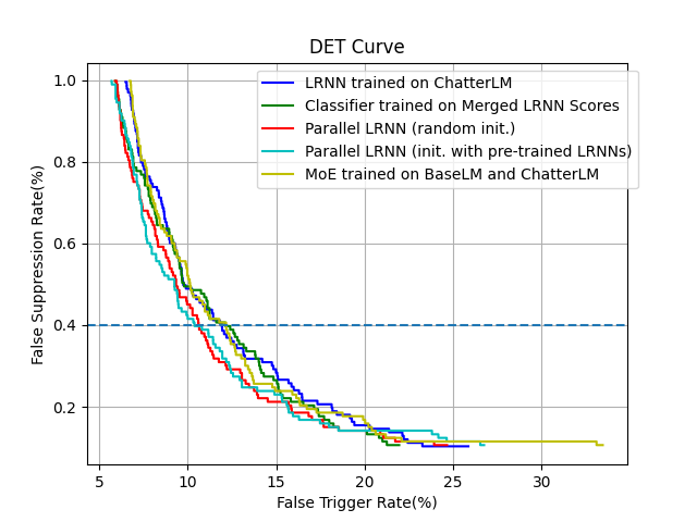
Figure 4: DET curves of ChatterLM and Ensemble of parallel Bi-LRNNs trained on BaseLM and ChatterLM

4 Conclusions

We proposed a novel solution to the ASR lattice based false trigger mitigation approach by introducing a complementary LM to the decoding process. The LM is trained from out-of-domain data sources and provides complementary information to the original LM optimized for in-domain ASR accuracy. We demonstrated that a Bi-LRNN classifier built from the lattices generated from the complementary LM significantly outperforms the classifier built from the baseline ASR model set. With this single ChatterLM Bi-LRNN, we achieved a $38.34\%$ relative reduction of the FT rate at the fixed $0.4\%$ FS level comparing to the current production FTM model. Furthermore, we proposed a novel approach of parallel Bi-LRNN, and examined multiple ways to implement and train the classifier. By back-propagating the training loss fully to the parallel Bi-LRNN network, we saw a further $10.8\%$ relative reduction of the FT rate. These results indicate that there is room for improving the traditional ASR decoder in the FTM task, and encourage us to reconsider the architecture design that can enable parallel LM decoding and parallel Bi-LRNN computation.

References

- [1] S. Sigtia, R. Haynes, H. Richards, E. Marchi, and J. Bridle, “Efficient Voice Trigger Detection for Low Resource Hardware,” in Proc. Interspeech, Sept 2018, pp. 2092–2096. [Online]. Available: http://dx.doi.org/10.21437/Interspeech.2018-2204
- [2] M. Wu, S. Panchapagesan, M. Sun, J. Gu, R. Thomas, S. N. Prasad Vitaladevuni, B. Hoffmeister, and A. Mandal, “Monophone-Based Background Modeling for Two-Stage On-Device Wake Word Detection,” in 2018 IEEE International Conference on Acoustics, Speech and Signal Processing (ICASSP), 2018, pp. 5494–5498.
- [3] A. H. Michaely, X. Zhang, G. Simko, C. Parada, and P. Aleksic, “Keyword Spotting for Google Assistant Using Contextual Speech Recognition,” in 2017 IEEE Automatic Speech Recognition and Understanding Workshop (ASRU), 2017, pp. 272–278.
- [4] S. Mallidi, R. Maas, K. Goehner, A. Rastrow, S. Matsoukas, and B. Hoffmeister, “Device-directed Utterance Detection,” in Proc. Interspeech, Sept 2018, pp. 1225–1228.
- [5] C.-W. Huang, R. Maas, S. H. Mallidi, and B. Hoffmeister, “A Study for Improving Device-Directed Speech Detection Toward Frictionless Human-Machine Interaction,” in Proc. Interspeech, Sept 2019, pp. 3342–3346. [Online]. Available: http://dx.doi.org/10.21437/Interspeech.2019-2840
- [6] F. Ladhak, A. Gandhe, M. Dreyer, L. Mathias, A. Rastrow, and B. Hoffmeister, “LatticeRnn: Recurrent Neural Networks Over Lattices,” in Proc. Interspeech, Sept 2016, pp. 695–699. [Online]. Available: http://dx.doi.org/10.21437/Interspeech.2016-1583
- [7] W. Jeon, L. Liu, and H. Mason, “Voice Trigger Detection from LVCSR Hypothesis Lattices Using Bidirectional Lattice Recurrent Neural Networks,” in 2019 IEEE International Conference on Acoustics, Speech and Signal Processing (ICASSP), May 2019, pp. 6356–6360.
- [8] P. Dighe, S. Adya, N. Li, S. Vishnubhotla, D. Naik, A. Sagar, Y. Ma, S. Pulman, and J. Williams, “Lattice-Based Improvements for Voice Triggering Using Graph Neural Networks,” in ICASSP 2020 - 2020 IEEE International Conference on Acoustics, Speech and Signal Processing (ICASSP), 2020, pp. 7459–7463.
- [9] R. Jacobs, M. I. Jordan, S. J. Nowlan, and G. E. Hinton, “Adaptive Mixtures of Local Experts,” Meual Computation, February 1991.
- [10] Z. Huang, T. Ng, L. Liu, H. Mason, X. Zhuang, and D. Liu, “SNDCNN: Self-Normalizing Deep CNNs with Scaled Exponential Linear Units for Speech Recognition,” in ICASSP 2020 - 2020 IEEE International Conference on Acoustics, Speech and Signal Processing (ICASSP), 2020, pp. 6854–6858.
- [11] K. Veselý, A. Ghoshal, L. Burget, and D. Povey, “Sequence Discriminative Training of Deep Neural Networks,” in Proc. Interspeech, Aug 2013.
- [12] G. Klambauer, T. Unterthiner, A. Mayr, and S. Hochreiter, “Self-Normalizing Neural Networks,” in Advances in Neural Information Processing Systems 30, 2017, pp. 971–980. [Online]. Available: http://papers.nips.cc/paper/6698-self-normalizing-neural-networks.pdf