A class of Finite difference Methods for solving inhomogeneous damped wave equations

Abstract.

In this paper, a class of finite difference numerical techniques is presented to solve the second-order linear inhomogeneous damped wave equation. The consistency, stability, and convergences of these numerical schemes are discussed. The results obtained are compared to the exact solution, ordinary explicit, implicit finite difference methods, and the fourth-order compact method (FOCM). The general idea of these methods is developed by using $C_{0}$-semigroups operator theory. We also showed that the stability region for the explicit finite difference scheme depends on the damping coefficient.

1. introduction

The damped wave equation is an important evolution model. Physicists and engineers widely use it in describing the propagation of water waves, sound waves, electromagnetic waves, etc. For instance, a model that describes the transverse vibrations of a string of a finite length in the presence of an external force proportional to the velocity satisfies the following partial differential equation (PDE)

(1) $$u_{tt}=\Delta u-\gamma(x)u_{t}+g(x,t),\hskip 10.0pt\text{for}\hskip 10.0pt~{}~{}~{}a\leq x\leq b,~{}~{}t\in R,$$

with initial conditions

$$u(x,0)=\phi(x),~{}~{}~{}~{}~{}~{}~{}~{}~{}u_{t}(0,x)=\psi(x),\hskip 10.0pt\text{for}~{}a\leq x\leq b,$$

and boundary conditions

$$u(a,t)=u_{a}(t)\hskip 10.0ptu(b,t)=u_{b}(t),\hskip 30.0pt~{}~{}~{}t\in R,$$

where $\gamma\geq 0$ is the damping force, $u(x,t)$ is the position of a point $x$ in the string, at instant $t$. The functions $\phi(x),\psi(x)$ and their derivatives are continuous functions of $x$ and the forcing function $g(x,t)\in L_{x}^{1}(\mathbb{R})$. The study of the numerical solution of this model will be our main focus in this article.

In general, the damping reduces the amplitude of vibration, and therefore, it is desirable to have some amount of damping to achieve stability in the system. One can find a detailed study in [4, 2, 14] of the effect of damping in the long-time stability of the equation (1). Also, for practical purposes, it is important to know how much damping is needed in the system to ensure the fastest decay rate in the amplitude of the wave as time evolves. For example, in the case of the 3D tsunami wave, we would like to know the size and structure of the damping force to bring the amplitude of the tsunami to a safe level before it hits the shore (see [17] and references within). In the case of the damping terms as a function of time and space, obtaining an analytic solution is a challenging problem. There comes the numerical study to find the approximate solution to such problems. In recent years, much attention has been given to studying the behaviours of the numerical solution of (1); see for example [18, 3, 13, 5, 8].

In this manuscript, we develop a class of methods based on the properties of $C_{0}$-semigroups of the evolution equations, as well as the finite difference method (FD). Generally speaking, the FD methods are easy to apply to partial differential equitations, but they may not lead to optimal results depending on the type of equation. The techniques used in this article take advantage of the $C_{0}$-semigroup property and Padé approximation, which lead to a better performance of new numerical schemes presented in this article.

At the time of writing this paper, we became aware of [12] that have a similar approach in which the authors drive a fourth-order implicit finite difference scheme to solve a second-order telegraph equation with constant coefficients. However, the author of [12] did not consider the explicit finite difference schemes and used the higher-order approximation terms of the space derivative and time integration to attain higher-order accuracy of the numerical solution. In this manuscript, in addition to driving a class of explicit and implicit methods, we discussed the issue of the instability of the explicit finite difference methods. Moreover, this paper explains the importance of the non-zero damping term in the existence of the stability region as well. We have also shown that the explicit finite difference method produces better results and costs a lot fewer calculations in its stability region.

An outline of the contents of this paper is as follows. In section 2, we set our numerical schemes and derive our method. Section 3 is devoted to the analytical properties of the method, i.e., consistency, stability, and convergence. Finally, in section 4, the numerical results of our method are compared with some of the existing methods.

2. The semigroup approach

To present a more convenient form of (1), we define a new vector function

(2) $$U(x,t)=(u,u_{t})^{T},\ \ U_{0}=(\phi(x),\psi(x))^{T}.$$

With these changes, the equation (1) turns into an evolution equation of first-order in time

(3) $$U_{t}=\mathcal{A}U+G,$$

where

$$\mathcal{A}=\left(\begin{array}[]{cc}0&I\\ \\ \ \Delta&-\gamma(x)\end{array}\right),\ \ \ \ G(x,t)=\left(\begin{array}[]{c}0\\ \\ g(x,t)\end{array}\right),$$

with initial condition

$$U(x,0)=\left(u(x,0),u_{t}(x,0)\right)^{T}.$$

The system above is defined on a Hilbert space $\mathcal{H}=H^{1}[a,b]\times L^{2}(\mathbb{R})$. The domain of $\mathcal{A}$ is $D(\mathcal{A})=H^{2}[a,b]\times H^{1}(\mathbb{R})$. Since $-\mathcal{A}$ is a dissipative and invertible operator on a Hilbert space, it generates a $C_{0}$-semigroup of contractions for $t\geq 0$ by the Lumber-Phillips theorem [10]. Also, note that the inclusion $D(\mathcal{A})\hookrightarrow\mathcal{H}$ is compact by the Rellich-Kondrachiv theorem. Thus, the spectrum of $\mathcal{A}$ contains only eigenvalues of finite multiplicity.

2.1. Discretization

We use the central discretization for the Laplacian operator $\Delta$ as

$$\Delta u(x,t)=\frac{u(x-h,t)-2u(x,t)+u(x+h,t)}{h^{2}}.$$

We set the mesh points

$$x_{i}=a+ih,~{}~{}i=0,1,2\dots N,~{}~{}~{}~{}~{}~{}~{}~{}~{}\text{where $h=\frac{b-a}{N}$}$$

of the interval $[a,b]$. Then the continuous operator $\mathcal{A}$ can be approximated by the matrix operator

$$\mathcal{M}_{(2N-2)}=\left[\begin{array}[]{cc}0&I\\ \\ \frac{1}{h^{2}}A&-\Gamma\end{array}\right],$$

where $I$ is the identity matrix of order $N-1$, and

(18) $$A=\left[\begin{array}[]{cccccc}-2&1&0&\cdots&0\\ \\ 1&-2&1&\cdots&0\\ 0&1&-2&\ddots&0\\ \vdots&\ddots&\ddots&\ddots&\vdots\\ 0&\cdots&0&1&-2\\ \end{array}\right]_{(N-1)\times(N-1)},\Gamma=\left[\begin{array}[]{cccc}\gamma(x_{1})&0&\cdots&0\\ \\ 0&\gamma(x_{2})&\dots&0\\ \\ 0&0&\cdots&0\\ \vdots&\ddots&\ddots&\vdots\\ 0&\cdots&0&\gamma(x_{N-1})\\ \end{array}\right]_{(N-1)\times(N-1).}$$

The discrete operator $\mathcal{M}_{(2N-2)}$ is defined on the finite-dimensional Banach space $X_{(2N-2)}=\mathbb{C}^{(2N-2)}[a,b]$.
Let $V_{2N-2}(t)=\left[\begin{array}[]{c}u(x_{1},t),u(x_{2},t)\dots u(x_{N-1},t),u_{t}(x_{1},t),\cdots u_{t}(x_{N-1})\end{array}\right]^{T}$ be a vector which discretizes the function $U(x,t)=(u(x,t),\partial_{t}u(x,t))$ over the interval $[x_{1},x_{N-1}]$, then (3) leads us to the following dynamical system

(28) $$\frac{dV_{2N-2}(t)}{dt}=\left[\begin{array}[]{cc}0&I\\ \\ \frac{1}{h^{2}}{A}&-\Gamma\end{array}\right]V_{2N-2}(t)+\left[\begin{array}[]{c}0\\ \\ G(t)\end{array}\right]+\left[\begin{array}[]{c}0\\ \\ \frac{1}{h^{2}}B(t)\end{array}\right],$$

where $G(t)=\left[g(x_{1},t),g(x_{2},t),\dots,g(x_{N-1},t)\right]^{T}$, $B(t)=\left[\begin{array}[]{c}u_{a}(t),0,0,\ldots,0,0,u_{b}(t)\end{array}\right]$ and the initial condition

$$V_{2N-2}(0)=\left[\begin{array}[]{c}\phi(x_{1}),\phi(x_{2})\dots\phi(x_{N-1}),\psi(x_{1}),\cdots\psi(x_{N-1})\end{array}\right]^{T}.$$

We will now drop the subscript $2N-2$ and write $V_{2N-2}(x,t)$ by $V(t)$, and $\mathcal{M}_{2N-2}$ by $\mathcal{M}$ in the rest of our presentation.

Since $\mathcal{M}$ is a bounded linear operator on a finite-dimensional space $X_{(2N-2)}\times H_{0}^{1}(\mathbb{R})$, it generates a $C_{0}$-semigroup for each $N$. Then, by using the $C_{0}$-semigroup theory of inhomogeneous evolution equations, we can construct the sequences of approximating solutions to (28) as

$$V(t)=e^{\mathcal{M}t}V(0)+\int_{0}^{t}e^{\mathcal{M}(t-s)}F(s)~{}ds,$$

where

$$F(t)=\left[\begin{array}[]{c}0\\ \\ G(t)\end{array}\right]+\left[\begin{array}[]{c}0\\ \\ \frac{1}{h^{2}}B(t)\end{array}\right].$$

We replace $t$ by $t+k$ in the above equation and use the $C_{0}$-semigroup property, $e^{\mathcal{M}(t+k)}=e^{\mathcal{M}t}e^{\mathcal{M}k}$, we get

$$V(t+k) = e^{\mathcal{M}(t+k)}V(0)+\int_{0}^{t+k}e^{\mathcal{M}(t+k-s)}F(s)~{}ds$$

$$= e^{\mathcal{M}k}e^{\mathcal{M}t}V(0)+e^{\mathcal{M}k}\int_{0}^{t}e^{\mathcal{M}(t-s)}F(s)~{}ds+e^{\mathcal{M}k}\int_{t}^{t+k}e^{\mathcal{M}(t-s)}F(s)~{}ds$$

$$= e^{\mathcal{M}k}\left(V(t)-\int_{0}^{t}e^{\mathcal{M}(t-s)}F(s)~{}ds\right)+e^{\mathcal{M}k}\int_{0}^{t}e^{\mathcal{\mathcal{M}}(t-s)}F(s)~{}ds$$

$$+ e^{\mathcal{M}k}\int_{t}^{t+k}e^{\mathcal{M}(t-s)}F(s)~{}ds.$$

Thus,

(31) $$V(t+k) = e^{\mathcal{M}(k)}V(t)+e^{\mathcal{M}k}\int_{t}^{t+k}e^{\mathcal{M}(t-s)}F(s)~{}ds.$$

To approximate the term $e^{\mathcal{M}k}$, we make use of the rational approximation of exponential functions, i.e., the Padé approximation.

2.2. Padé Approximant

The Padé approximation is a rational approximation of a function of a given order [1]. The technique was developed around 1890 by Henri Padé, but it goes back to F. G. Frobenius who introduced the idea and investigated the features of rational approximations of power series. The Padé approximation is usually superior when functions contain poles because the use of rational function allows them to be well represented. The Padé approximation often gives a better approximation of the function than truncating its Taylor series, and it may still work where the Taylor series does not converge.

Padé approximation gives the exponential functions $e^{\theta}$ as

$$e^{\theta}=\frac{1+a_{1}\theta+a_{2}\theta^{2}+\cdots+a_{T}\theta^{T}}{1+b_{1}\theta+b_{2}\theta^{2}+\cdots+_{T}\theta^{S}}+c_{S+T+1}\theta^{S+T+1}+O(\theta^{S+T+2}),$$

where $C_{S+T+1}$, $a_{i}$’s and $b$’s are constants. The rational function

(32) $$R_{S,T}(\theta):=\frac{1+a_{1}\theta+a_{2}\theta^{2}+\cdots+a_{T}\theta^{T}}{1+b_{1}\theta+b_{2}\theta^{2}+\cdots+_{T}\theta^{S}}=\frac{P_{T}(\theta)}{Q_{S}(\theta)}$$

is the so-called Padé approximation of order $(S,T)$ to $e^{\theta}$ with the leading error $c_{S+T+1}\theta^{S+T+1}$. The table below gives some Padé approximations of the exponential function[18].

$$\begin{array}[]{p{2in}p{3in} p{2in} }\hline\cr\hline\cr\vskip 2.0pt\centering(S,T)\@add@centering&\vskip 2.0pt\centering$R_{S,T}(\theta)$\@add@centering&\vskip 2.0pt$\text{Leading error}$\vskip 3.0pt\\ \hline\cr\centering\vskip 2.0pt(0,1)\@add@centering&\centering\vskip 2.0pt$1+\theta$\@add@centering&\vskip 2.0pt$\frac{1}{2}\theta^{2}$\vskip 3.0pt\\ \centering\vskip 2.0pt(0,2)\@add@centering&\centering\vskip 2.0pt$1+\theta+\frac{1}{2}\theta^{2}$\@add@centering&\vskip 2.0pt$\frac{1}{6}\theta^{3}$\vskip 3.0pt\\ \centering\vskip 2.0pt(1,0)\@add@centering&\centering\vskip 2.0pt$\dfrac{1}{1-\theta}$\@add@centering&\vskip 2.0pt$-\frac{1}{2}\theta^{2}$\vskip 3.0pt\\ \centering\vskip 2.0pt(1,1)\@add@centering&\centering\vskip 2.0pt$\dfrac{1+\frac{1}{2}\theta}{1-\frac{1}{2}\theta}$\@add@centering&\vskip 2.0pt$-\frac{1}{12}\theta^{3}$\vskip 3.0pt\\ \hline\cr\hline\cr\end{array}$$

Now combining (2.1) and (32), we get

$$Q_{S}(\mathcal{M}k)V(t+k) = P_{T}(\mathcal{M}k)V(t)$$

$$+ P_{T}({\mathcal{M}k})\int_{t}^{t+k}P_{T}({\mathcal{M}(t-s)})(Q_{S}({\mathcal{M}(t-s)}))^{-1}F(s)~{}ds.$$

For the integration term on the right-hand side, one can use the numerical integration formula. Here, we will use the Trapezoidal approximation of integration to get the following numerical scheme

(34) $$Q_{S}(\mathcal{M}k)V(t+k) = P_{T}(\mathcal{M}k)V(t)+\frac{k}{2}P_{T}(\mathcal{M}k)F(t)+\frac{k}{2}Q_{S}(\mathcal{M}k)F(t+k).$$

This is the general form of our scheme, and each choice of $Q_{S}$ and $P_{T}$ produces explicit and implicit finite difference methods to the solution of the damped wave equation (1). Next, we present two schemes by taking $(S,T)=(0,1)$ and $(S,T)=(1,1)$. Similarly, we can develop more schemes of different order by taking different values of $S$ and $T$ mentioned in the table above.
Explicit Method ($FD-(0,1)$): If we set $(S,T)=(0,1)$ i.e. $Q_{0}(\theta)=1$ and $P_{1}(\theta)=1+\theta$ in (34), we will obtain the FD-(0,1) as

(35) $$\begin{cases}V{(t+k)}=(1+\mathcal{M}k)V{(t)}+\frac{k}{2}(I+\mathcal{M}k)F(t)+\frac{k}{2}F(t+k),\\ V^{0}=[u_{1}(0),\cdots,u_{N-1}(0),\partial_{t}u_{1}(0),\cdots,\partial_{t}u_{N-1}(0)].\end{cases}$$

Implicit Method ($FD-(1,1)$): By a choice of $P_{1}(\theta)=1+\frac{1}{2}\theta$ and $Q_{1}(\theta)=1-\frac{1}{2}\theta$ in (34), we will obtain the FD-(1,1) as

(36) $$\begin{cases}\left(1-\frac{1}{2}\mathcal{M}k\right)V(t+k)=\left(1+\frac{1}{2}\mathcal{M}k\right)V(t)+\frac{k}{2}\left(I+\frac{1}{2}\mathcal{M}k\right)F(t)\\ \hskip 80.00012pt+\frac{k}{2}\left(I-\frac{1}{2}\mathcal{M}k\right)F(t+k),\\ V^{0}=[u_{1}(0),\cdots,u_{N-1}(0),\partial_{t}u_{1}(0),\cdots,\partial_{t}u_{N-1}(0)].\end{cases}$$

In the case of the implicit method, we need to solve a more extensive system of equations in each time step due to the implicit nature of the system. However, the analysis and numerical results suggest that the implicit scheme gives us an accurate approximation and, more importantly, an unconditionally stable scheme.

3. Consistency, Stability and Convergence

In this section, we will investigate the analytical properties of our numerical schemes (35) and (36). We will prove that the numerical methods (35) and (36) are consistent, stable, and hence convergent. We will use the direct analysis to prove the consistency, the matrix method to prove the stability, and the Lax-equivalence theorem to prove the convergence of our numerical schemes.

3.1. Consistency

Given a partial differential equation $Lu=f$ and a finite difference scheme, $F_{h,k}v=f$, we say that the finite difference scheme is consistent with the partial differential equation if for any smooth function $\phi(x,t)$,

$$L\phi-F_{h,k}\phi\to 0~{}~{}\text{as}~{}~{}h,k\to 0,$$

or in other words, the local truncation goes to zero as the mesh size $h$ and $k$ tends to zero. The partial differential equation

$$U_{t}-\left(\begin{array}[]{cc}0&I\\ \\ \ \Delta&-\gamma(x)\end{array}\right)U-\left(\begin{array}[]{c}0\\ \\ g(x,t)\end{array}\right)=0,$$

is approximated at the point $(x_{i},t)$ by the $n^{th}$ row of the following difference equations

$$\frac{1}{k}\left(Q_{S}({\mathcal{M}k})V(t+k)-P_{T}({\mathcal{M}k})V(t)\right)-\frac{1}{2}P_{T}({\mathcal{M}k})F(t)-\frac{1}{2}Q_{S}({\mathcal{M}k})F(t+k)=0,$$

for $n=1,2,\cdots,(2N-2).$
Then the local truncation error $T_{i,t}(U)$ is defined as the $n^{th}$ row of

$$\frac{1}{k}\left(Q_{S}({\mathcal{M}k})U(t+k)-P_{T}({\mathcal{M}k})U(t)\right)-\frac{1}{2}P_{T}({\mathcal{M}k})F(t)-\frac{1}{2}Q_{S}({\mathcal{M}k})F(t+k),$$

for $n=1,\cdots,(2N-2)$.
The truncated error depends on the choice of $Q_{S}$ and $P_{T}$. Therefore, we should consider them case by case. Here we consider $FD-(0,1)$ and $FD-(1,1)$. The remaining cases follow the same path.

3.1.1. $FD-(0,1)$

The local truncation error $T^{0,1}_{i,t}(U)$ of the explicit $FD-(0,1)$ is defined as the $n^{th}$ row of

$$\frac{1}{k}\left(U(t+k)-(I+{\mathcal{M}k})U(t)\right)-\frac{1}{2}(I+{\mathcal{M}k})F(t)-\frac{1}{2}F(t+k)$$

for $n=1,2\cdots,(2N-2)$.
Thus for $i=1,2,\cdots N-1$, we get the following system of $(2N-2)$ equations

$$T^{0,1}_{i,t}(U)=\frac{1}{k}\left(u(x_{i},t+k)-u(x_{i},t)\right)-u_{t}(x_{i},t)-\frac{k}{2}g(x_{i},t),$$

and

$$T^{0,1}_{i+N-1,t}(U)=\frac{1}{k}u_{t}(x_{i},t+k)-\frac{1}{h^{2}}(u(x_{i}-h,t)-2u(x_{i},t)+u(x_{i}+h,t))$$

$$-{\frac{1}{k}(1-k\gamma(x_{i}))u_{t}(x_{i},t)}-~{}\frac{(1-\gamma(x_{i})k)}{2}g(x_{i},t)-\frac{1}{2}g(x_{i},t+k).$$

By Taylor series expansion, we get

$$T^{0,1}_{i,t}(U)=\frac{k}{2!}u_{tt}(x_{i},t)+\frac{k^{2}}{3!}u_{ttt}(x_{i},t)+\cdots-\frac{k}{2}g(x_{i},t)$$

and

$$T^{0,1}_{i+N-1,t}(U) = \left(u_{tt}(x_{i},t)-u_{xx}(x_{i},t)+\gamma(x_{i})u_{t}(x_{i},t)-g(x_{i},t)\right)$$

$$+\frac{k}{2!}u_{ttt}(x_{i},t)+O(k^{2})-\frac{2h^{2}}{4!}u_{xxxx}(x_{i},t)+O(h^{4})+\frac{\gamma(x_{i})k}{2}g(x_{i},t)$$

$$-\frac{k}{2}g_{t}(x_{i},t)+O(k^{2}).$$

for  $i=1,2,\cdots,(N-1)$.
By (1), the last ($N-1$), equations can be written as

$$T^{0,1}_{i,t}(U) = \frac{k}{2!}u_{ttt}(x_{i},t)+O(k^{2})-\frac{2h^{2}}{4!}u_{xxxx}(x_{i},t)+O(h^{4})+\frac{\gamma(x_{i})k}{2}g(x_{i},t)$$

$$- \frac{k}{2}g_{t}(x_{i},t)+O(k^{2}).$$

We observe as $h$ and $k$ go to zero, the truncation error $T_{i,t}(U)\to 0$. Hence, the numerical scheme is consistent. .

3.1.2. $FD-(1,1)$

The local truncation error $T^{1,1}_{i,t}(U)$ of the explicit $FD-(1,1)$ is defined as the $n^{th}$ row of

$$\frac{1}{k}\left(\left(I-\frac{1}{2}{\mathcal{M}k}\right)U(t+k)-\left(I+\frac{1}{2}{\mathcal{M}k}\right)U(t)\right)-\frac{1}{2}\left(I+\frac{1}{2}{\mathcal{M}k}\right)F(t)-\frac{1}{2}\left(I-\frac{1}{2}{\mathcal{M}k}\right)F(t+k)$$

for $n=1,2,\cdots,(2N-2)$.
Thus for $i=1,2\cdots,N-1$, we get the following system of $(2N-2)$ equations

$$T^{1,1}_{i,t}(U)=\frac{1}{k}\left(u(x_{i},t+k)-u(x_{i},t)\right)-u_{t}(x_{i},t)-\frac{k}{4}\left(g(x_{i},t+k)-g(x_{i},t)\right),$$

and

$$T^{1,1}_{i+N-1,t}(U) = \left[-\frac{1}{2h^{2}}\left(u(x_{i}-h,t+k)-2u(x_{i},t+k)+u(x_{i}+h,t+k)\right)+\frac{1}{k}\left(1+\frac{\gamma k}{2}\right)u_{t}(x_{i},t+k)\right]$$

$$-\left[\frac{1}{2h^{2}}\left(u(x_{i}-h,t)-2u(x_{i},t)+u(x_{i}+h,t)\right)+\frac{1}{k}\left(1-\frac{\gamma k}{2}\right)u_{t}(x_{i},t)\right]$$

$$-\frac{1}{2}\left[(1+\frac{\gamma k}{2})g(x_{i},t)+(1-\frac{\gamma k}{2})g(x_{i},t+k)\right].$$

By Taylor series expansion, we get

$$T^{1,1}_{i,t}(U)=\frac{k}{2}u_{tt}(x_{i},t)-\frac{k^{2}}{4}g_{t}(x_{i},t)+O(k^{3}),$$

and

$$T^{1,1}_{i+N-1,t}(U) = \left(u_{tt}(x_{i},t)-u_{xx}(x_{i},t)+\gamma(x_{i})u_{t}(x_{i},t)-g(x_{i},t)\right)$$

$$+ \frac{k}{2}u_{ttt}(x_{i},t)+O(k^{2})-\frac{k}{2}u_{xxt}(x_{i},t)+{O}(k^{2})-\frac{h^{2}}{2}u_{xxxx}(x_{i},t)+O(h^{4})$$

$$- \frac{kh^{2}}{6}u_{xxxxt}+h^{2}O(k^{2})-\frac{k}{2}g_{t}(x_{i},t)+O(k^{2})+\frac{k^{3}\gamma(x_{i})}{4}g_{t}(x_{i},t)+O(k^{3}),$$

for $i=1,2,\cdots,(N-1)$.
By (1), the last ($N-1$), equations can be written as

$$T^{1,1}_{i,t}(U) = \frac{k}{2}u_{ttt}(x_{i},t)+O(k^{2})-\frac{k}{2}u_{xxt}(x_{i},t)+{O}(k^{2})-\frac{h^{2}}{2}u_{xxxx}(x_{i},t)+O(h^{4})$$

$$- \frac{kh^{2}}{6}u_{xxxxt}+h^{2}O(k^{2})-\frac{k}{2}g_{t}(x_{i},t)+O(k^{2})+\frac{k^{3}\gamma(x_{i})}{4}g_{t}(x_{i},t)+O(k^{3}).$$

As $h$ and $k$ go to zero, the truncation error $T_{i,t}(U)\to 0$. Hence, the numerical scheme is consistent.

3.2. Stability

To prove the stability of our numerical schemes, we show that there exists a region $\Lambda$ so that for every $h,k\in\Lambda$, all the eigenvalues of the amplification matrix related to the numerical schemes lie in or on the unit circle.

Proposition 1.

The explicit FD-(0,1) approximation defined in (34) is stable for $k<\frac{2}{\gamma_{*}}$ and $\frac{\sqrt{k}}{h}<\frac{\sqrt{\gamma_{*}}}{2}$, where $\gamma_{*}=\max_{x\in[a,b]}\gamma(x)$.

The following lemma will be used to prove Proposition 1.

Lemma 1.

Let $p(x)=ax^{2}+bx+c$ be a polynomial function with $a>0$, then necessary and sufficient conditions for the polynomial $p(x)$ to have the modulus of its roots less or equal to 1 are

• $|c|<a$

• $p(1)>0$ and $p(-1)>0$.

One can find the proof of the above lemma in [7, 16].
Proof of proposition 1. The eigenvalues of the amplification matrix $I+k\mathcal{M}$ are the roots of the following quadratics equation

$$\lambda^{2}+(-2+\gamma(x_{n})k)\lambda+1-k\gamma(x_{n})+4r^{2}\sin^{2}\left(\frac{n\pi}{2N}\right)=0,\ \ n=1,\cdots,(N-1),$$

where $r=k/h$.
Note for each $n$, there are two roots of the above polynomial, and hence we have $2N-2$ eigenvalues for the matrix $I+k\mathcal{M}$.
Next, in order to satisfy the conditions $(i)$ and $(ii)$ of lemma (1), we impose restrictions on $\gamma_{*}$ and $r$. Indeed, the assumption $(i)$ is satisfied if

$$-1<1-k\gamma(x_{n})+4r^{2}\sin^{2}\left(\frac{n\pi}{2N}\right)<1,~{}~{}~{}n=1,2,\cdots,N-1.$$

The right-hand inequality gives us

$$4r^{2}\sin^{2}\left(\frac{n\pi}{2N}\right)<k\gamma(x_{n})\leq k\gamma_{*},$$

$$r^{2}<\frac{k\gamma_{*}}{4\sin^{2}\left(\frac{n\pi}{2N}\right)}.$$

Thus, $\frac{\sqrt{k}}{h}<\frac{\sqrt{\gamma_{*}}}{2}$.
Now, the first part of the assumption (ii) is satisfied if

$$p(1)=4r^{2}\sin^{2}\left(\frac{n\pi}{2N}\right)>0,$$

which is true as long as $r>0$.
Now, the second part of assumption (ii) is satisfied if

$$p(-1)=4-2k\gamma(x_{n})+4r^{2}\sin^{2}\left(\frac{n\pi}{2N}\right)>0,$$

which is true if

$$k\gamma_{*}<2.$$

Hence the second part of the assumption (ii) of lemma (1) is satisfied for $k<\frac{2}{\gamma_{*}}$.

Proposition (1) tells us that the damping term plays an important role in the stability of the explicit method (34). The finite difference scheme (34) will be unstable for any values of $h$ and $k$ if the damping term $\gamma(x)$ is identically zero or $h$ and $k$ are out of the required bounds of the proposition (1).

Proposition 2.

The implicit FD-(1,1) approximation defined by (36) is unconditionally stable.

Proof.

The eigenvalues of the matrix $\mathcal{M}$ are given by

$$\lambda_{n}^{\pm}=-\frac{\gamma(x_{n})}{2}\pm\frac{1}{2}\sqrt{\gamma(x_{n})^{2}-\frac{16}{h^{2}}\sin^{2}(\frac{n\pi}{2N})},~{}~{}~{}~{}~{}~{}n=1,\cdots,N-1.$$

Then, by using functional calculus, the eigenvalues $\mu_{n}^{\pm}$ of the matrix $(I-\frac{1}{2}k\mathcal{M})^{-1}((I+\frac{1}{2}k\mathcal{M}))$ are given by

$$\mu_{n}^{\pm}=\frac{1+\frac{k}{2}\lambda_{n}^{\pm}}{1-\frac{k}{2}\lambda_{n}^{\pm}},\ \ n=1,\cdots,N-1.$$

Also, we have $Re(\lambda_{n})\leq 0$ because $\gamma\geq 0$. Thus, for any values of $n,h,k$, and $\gamma(x_{n})$, we get $|\mu_{n}^{\pm}|\leq 1$. Hence, the implicit method (36) is unconditionally stable. ∎

A direct application of the Lax Equivalence Theorem [9, 15] leads to the convergence of our models.

Corollary 1.

The finite difference explicit $FD-(0,1)$ of (34) and implicit $FD-(1,1)$ of (36) are convergent.

4. Performance of Numerical schemes

In this section, we will see the performance of each finite difference scheme on a sample problem.
Sample Problem: We consider the following damped wave equation

$$u_{tt}=u_{xx}-2u_{t},$$

over the region $\Omega=[0\leq x\leq\pi]\times(t>0)$ with initial conditions

$$u(x,0)=\sin(x),\hskip 30.0ptu_{t}(x,0)=-\sin(x),$$

and boundary conditions

$$u(0,t)=0=u(\pi,t),\;\;\text{for}~{}t>0.$$

The exact solution of the above problem is $u(x,t)=e^{-t}\sin(x)$.

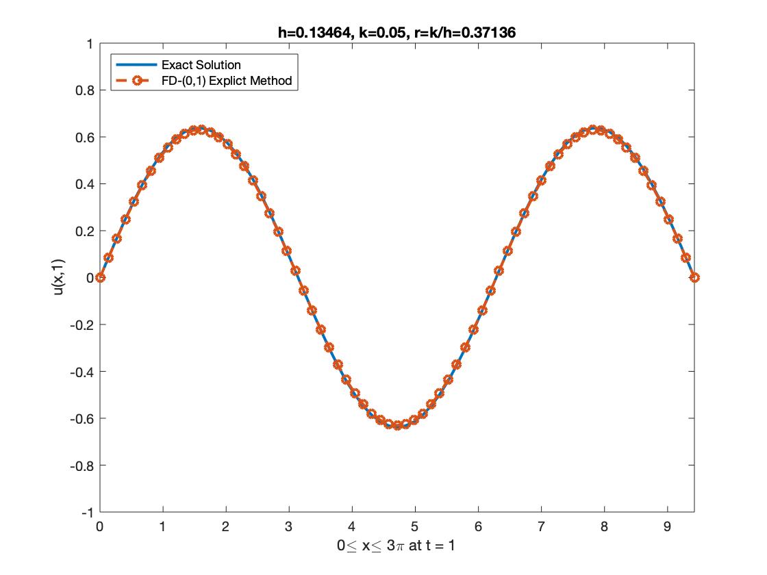
Figure 1. The approximate solution given by explicit FD-(0,1) of (35) at $t=1$ with $k=0.05$, $h=0.13464$.

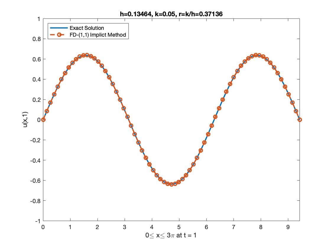
Figure 2. The approximate solution given by implicit FD-(1,1) of (36) at $t=1$ with $k=0.05$, $h=0.13464$.

FIGURE (1) and (2) show the numerical solutions using finite difference methods (34) and (36) at $t=1$. From the obtained numerical results, we can conclude that the numerical solutions are in good agreement with the exact solution.

4.1. Comparison with other methods

In this section, we compare our result with the ordinary explicit and implicit finite difference methods mentioned below. We also compare our result with the FOCM method of [6]. We take the same test example mentioned above for this comparison.
Ordinary Explicit Finite Difference Scheme (OEFD): The ordinary explicit finite difference scheme in the matrix form is

(38) $$(1+\frac{\gamma k}{2})u(t+k)=(2I-r^{2}A)u(t)+\left(\frac{\gamma k}{2}-1\right)u^{n-1}+r^{2}B(t),$$

where $r=k/h$, $B(t)=\left[\begin{array}[]{c}u_{a}(t),0,0,\ldots,0,0,u_{b}(t)\end{array}\right]$, and the matrix $A$ is defined in equation (18).
Ordinary Implicit Finite Difference Scheme(OIFD): The ordinary implicit finite difference scheme in the matrix form is

(39) $$\left(1+\frac{\gamma(x_{n})k}{2}-\frac{r^{2}}{2}A\right)u(t+k)=\left(2+\frac{r^{2}}{2}A\right)u(t)+\left(\frac{\gamma(x_{n})k}{2}-1\right)u(t-k)$$

$$+\frac{r^{2}}{2}\left(B(t+k)+B(t)\right),$$

where $r=k/h$, $B(t)=\left[\begin{array}[]{c}u_{a}(t),0,0,\ldots,0,0,u_{b}(t)\end{array}\right]$, and the matrix $A$ is defined in equation (18). The derivation of these schemes can be found in [11].

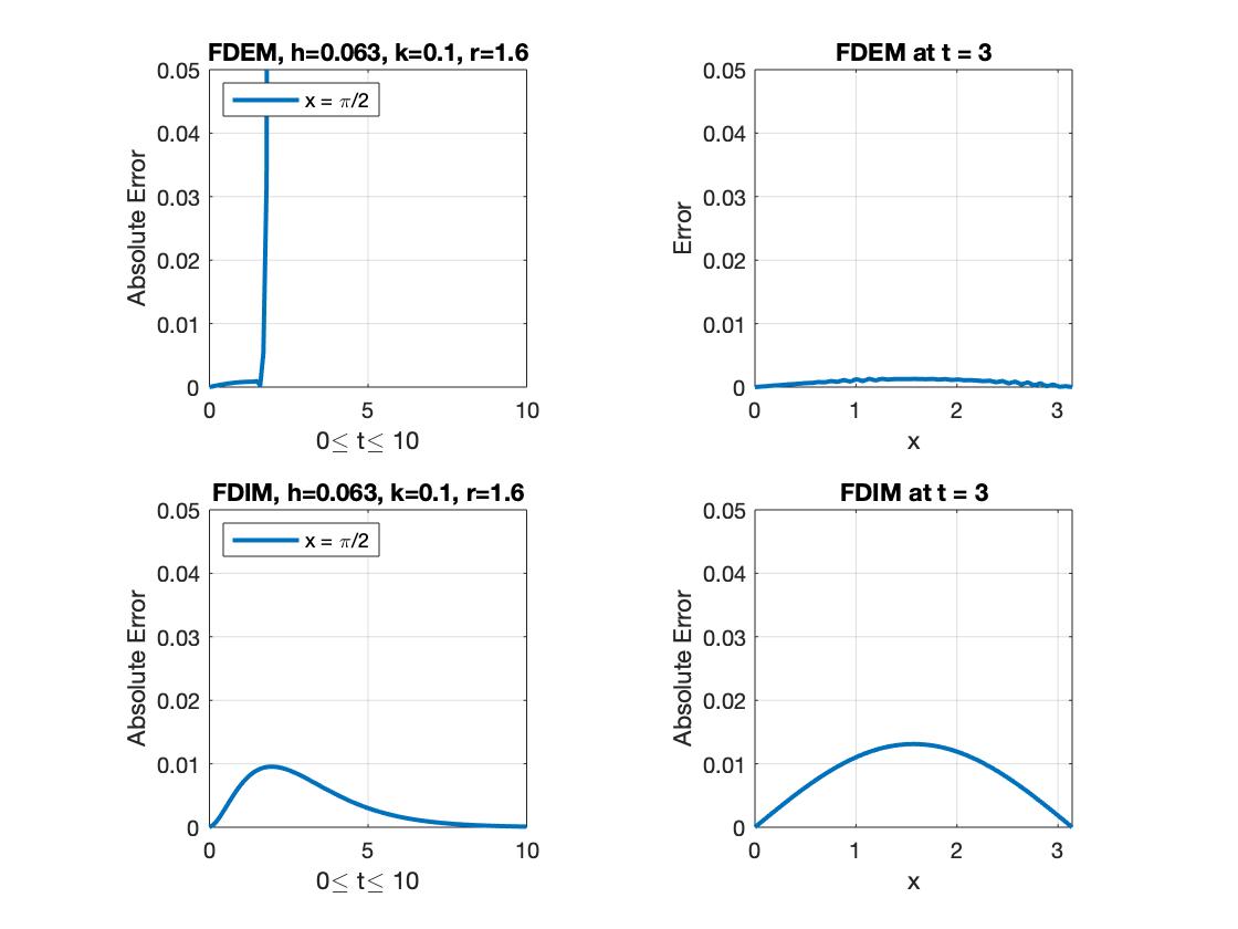
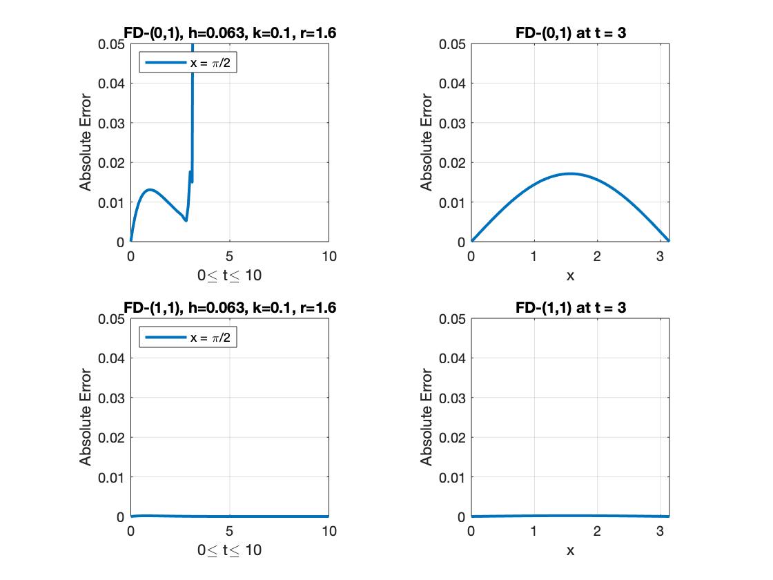
FIGURE (3) and (4) show the performances of our methods (35) and (36) in comparison with finite difference schemes (38) and (39) using $k=0.01$ and $h=0.063$. The implicit FD-(1,1) produces a much better result even for a large value of $r$. When the values of $h$ and $k$ fail to satisfy the stability conditions of the explicit FD-(0,1), it can be seen that the numerical solution became unstable after some time iterations. However, it is interesting to see that even in this case the global numerical solution fails to exist, the local numerical solution does exist for a small time and it was very close to the exact solution. It is apparent that the explicit finite difference scheme (38) and (34) are not stable for large values of $r$. The implicit FD-(1,1) is very stable and produces a much better result when compared to the ordinary implicit finite difference scheme (39).

Figure 3. The absolute error of the method (35) and (36) for $r=1.5915$.

Figure 4. The absolute error of the method (38) and (39) for $r=1.5915$.

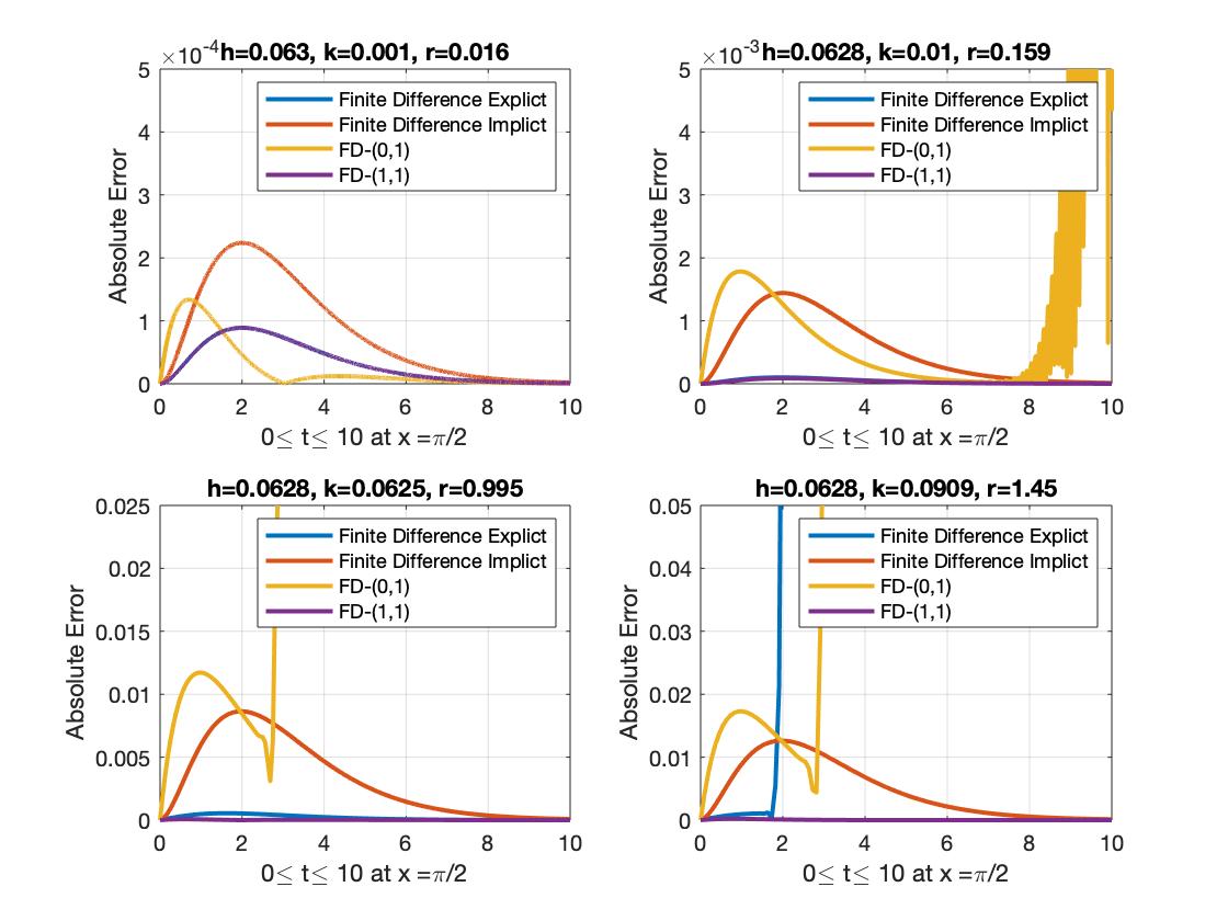
Figure 5. The absolute error of the method (35), (36), (38) and (39).

In the FIGURE (5), we plotted the absolute error at the four different values of $r=.016$, $r=.159$, $r=.995$, and $r=1.45$. One can see for a small values of $r=0.016$, all the four schemes produce fairly stable results. This shows that when our explicit finite difference FD-(0,1) satisfies the assumptions of proposition (1), it is stable and produces better results than the other three. However, the performances of the explicit finite difference method (34) and implicit finite difference FD-(1,1) (36) are very similar for small values of $r$.

$x$	FOCM	OEFD	OIFD	EX-(0,1)	IM-(1,1)
0	0	0	0	0	0
0.314159265	0.00012256	6.29067E-05	0.000135485	0.001494844	1.23932E-05
0.628318531	0.00022777	0.000119656	0.000257708	0.002843363	2.35734E-05
0.942477796	0.00031458	0.000164692	0.000354705	0.003913553	3.24459E-05
1.256637061	0.00036955	0.000193607	0.000416981	0.004600658	3.81425E-05
1.570796327	0.00038865	0.00020357	0.000438439	0.004837418	4.01054E-05
1.884955592	0.00036955	0.000193607	0.000416981	0.004600658	3.81425E-05
2.199114858	0.00031458	0.000164692	0.000354705	0.003913553	3.24459E-05
2.513274123	0.00022777	0.000119656	0.000257708	0.002843363	2.35734E-05
2.827433388	0.00012256	6.29067E-05	0.000135485	0.001494844	1.23932E-05
3.141592654	0	0	0	0	0

Table 1. Absolute Error

$r$	EFD	IFD	EX-(0,1)	IM-(1,1)
1.59	1.00967E+34	0.002547509	9.08234E+13	2.231E-06
0.53	3.05424E-05	0.00079153	2.18322E+11	1.36036E-05
0.32	2.04246E-05	0.000473008	3410.243641	1.43835E-05
0.23	1.76452E-05	0.000339697	0.011310925	1.45754E-05
0.18	1.64986E-05	0.000266457	7.84447E-05	1.46457E-05

Table 2. Maximum Error at $t=6$

TABLE 1 shows the comparison between the errors generated by FOCM, OEFD, OIFD, $EX-(0,1)$ and $IM-(1,1)$ at $t=0.3$ with $h=\frac{\pi}{10}$ and $k=\frac{1}{10}$.

TABLE 2 shows the magnitude of the maximum error at time $t=6$ between the exact solution and the numerical solution obtained by using FOCM, OEFD, OIFD, $FD-(0,1)$, and $FD-(1,1)$ discussed above with different values of $h$ and $k$.

5. Conclusion

In this paper, a class of finite difference methods using the $C_{0}$-semigroup operator theory for solving the inhomogeneous damped wave equation is presented. The stability and consistency of the implicit and explicit methods are proved. Test examples are presented, and the results obtained are compared with the exact solutions. The comparison certifies that implicit FD-(1,1) gives good results. Summarizing these results, we can say the general form of the new finite difference methods has a reasonable amount of calculations and the form is easy to use. All results are obtained by using MATLAB version 9.7.

References

• [1] GA Baker and PR Graves-Morris. Padé approximants, part i, encycl. math., vol. 13. Reading, MA: Addison-Wesley, 7:233–236, 1981.
• [2] Nicolas Burq and Romain Joly. Exponential decay for the damped wave equation in unbounded domains. Communications in Contemporary Mathematics, 18(06):1650012, 2016.
• [3] Ian Christie, David F Griffiths, Andrew R Mitchell, and Olgierd C Zienkiewicz. Finite element methods for second order differential equations with significant first derivatives. International Journal for Numerical Methods in Engineering, 10(6):1389–1396, 1976.
• [4] Lawrence C. Evans. Partial differential equations. American Mathematical Society, Providence, R.I., 2010.
• [5] Feng Gao and Chunmei Chi. Unconditionally stable difference schemes for a one-space-dimensional linear hyperbolic equation. Applied Mathematics and Computation, 187(2):1272–1276, 2007.
• [6] M.T. Hussain, A. Pervaiz, Zainulabadin Zafar, and M.O. Ahmad. Fourth order compact method for one dimensional homogeneous damped wave equation. Pakistan Journal of Science, 64(2):122, 2012.
• [7] Eliahu Jury. On the roots of a real polynomial inside the unit circle and a stability criterion for linear discrete systems. IFAC Proceedings Volumes, 1(2):142–153, 1963.
• [8] Stig Larsson, Vidar Thomée, and Lars B Wahlbin. Finite-element methods for a strongly damped wave equation. IMA journal of numerical analysis, 11(1):115–142, 1991.
• [9] Peter D Lax and Robert D Richtmyer. Survey of the stability of linear finite difference equations. Communications on pure and applied mathematics, 9(2):267–293, 1956.
• [10] Gunter Lumer and Ralph S Phillips. Dissipative operators in a banach space. Pacific Journal of Mathematics, 11(2):679–698, 1961.
• [11] Andrew Ronald Mitchell and David Francis Griffiths. The finite difference method in partial differential equations. Wiley. New York, 1980.
• [12] Akbar Mohebbi. A fourth-order finite difference scheme for the numerical solution of 1d linear hyperbolic equation. Commun. Numer. Anal, 2013.
• [13] Ahmet Özkan Özer and E İnan. One-dimensional wave propagation problem in a nonlocal finite medium with finite difference method. In Vibration Problems ICOVP 2005, 383–388. Springer, 2006.
• [14] Jeffrey Rauch, Michael Taylor, and Ralph Phillips. Exponential decay of solutions to hyperbolic equations in bounded domains. Indiana university Mathematics journal, 24(1):79–86, 1974.
• [15] Robert D Richtmyer and Keith W Morton. Difference methods for initial-value problems. dmiv, 1994.
• [16] Paul A Samuelson. Conditions that the roots of a polynomial be less than unity in absolute value. The Annals of Mathematical Statistics, 12(3):360–364, 1941.
• [17] Harvey Segur. Waves in shallow water, with emphasis on the tsunami of 2004. In Tsunami and nonlinear waves, 3–29. Springer, 2007.
• [18] Gordon Smith. Numerical solution of partial differential equations: finite difference methods. Oxford university press, 1985.