IFJPAN-IV-2020-6
All-plus helicity off-shell gauge invariant multigluon amplitudes at one loop

Abstract

We calculate one loop scattering amplitudes for arbitrary number of positive helicity on-shell gluons and one off-shell gluon treated within the quasi-multi Regge kinematics. The result is fully gauge invariant and possesses the correct on-shell limit. Our method is based on embedding the off-shell process, together with contributions needed to retain gauge invariance, in a bigger fully on-shell process with auxiliary quark or gluon line.

1 Introduction

Despite the high energy limit of Quantum Chromodynamics (QCD) (see eg. [1] for a review) has been studied for over forty years, the confrontation of various small-$x$ approaches and experimental data is still not fully conclusive (here $x\sim 1/\sqrt{s}$ is the longitudinal fraction of hadron momentum carried by a parton and $s$ is the center-of-mass energy). On one hand, the experimental data relevant to the small-$x$ regime can be often explained by the collinear factorization, supplemented however with parton showers or other type of resummations and multi-parton interactions. On the other hand, certain types of reactions, for example the Mueller-Navalet jet production [2] give strong hints towards the need of inclusion of the small-$x$ effects [3]. In addition, collisions of protons with heavy nuclei provide further hints, as observed for instance in [4] for the forward dijet production case.

In order to provide more solid statements regarding the need of small-$x$ approaches, one needs higher order corrections for various components of small-$x$ calculations, in particular for high energy partonic amplitudes. As a matter of fact, in collinear factorization, any partonic amplitude can be at present calculated at NLO automatically using computer software. This is still to be achieved in the small-$x$ domain and our work is a step forward towards that goal.

The key result in the small-$x$ field is the Balitsky-Fadin-Kuraev-Lipatov (BFKL) equation [5, 6], which describes evolution in energy (or $x$) of the gluon Green function in the high energy limit. It can also be converted to the energy evolution of so-called unintegrated parton distribution functions, that unlike collinear PDFs, explicitly depend on the parton transverse momentum $k_{T}$. Other key results in the small-$x$ QCD constitute the $k_{T}$-factorization (called also high energy factorization) [7, 8], as well as further developments that overcome the unitarity bound violation by the BFKL equation and lead to the nonlinear evolution of Balitsky-Kovchegov (BK) equation [9, 10], B-JIMWLK equations [9, 11, 12, 13, 14, 15, 16, 17, 18] and Color Glass Condensate (CGC) effective theory (see e.g. [19]). Some key higher order results include: the next-to-leading order (NLO) BFKL kernel [20, 21, 22], the NLO BK kernel [23], the B-JIMWLK equation at NLO [24, 25], the $\gamma^{*}\rightarrow\bar{q}q$ impact factor at NLO [26, 27, 28, 29] also with heavy quarks [30], partial inclusion of NLO for Higgs + jet [31], single inclusive jet production in CGC at NLO [32], and also the recent calculation of $\gamma^{*}\rightarrow\bar{q}q\gamma$ impact factor at NLO [33]. In addition, there are NLO calculations in the context of the Lipatov’s effective action [34, 35, 36, 37, 38, 39].

The concept of $k_{T}$-factorization is based on analogy with the collinear factorization, but here both a hard part and a soft hadronic part depend on theparton transverse momenta, i.e. we have explicit higher powers $k_{T}/Q$ present in the hard matrix elements (here, $Q$ is the largest scale present in the process). Thus, instead of the leading twist, the accuracy is set by the leading power in $1/\sqrt{s}$. The momenta of partons defining the hard amplitude may now be off-shell, with vector or spinor indices projected onto components dominating in the high energy limit.

In the present work we shall consider multigluon amplitudes with a single gluon being off mass shell. Such amplitudes are primarily used in the forward particle production (see eg. [40]) and have large phenomenological impact (see eg. [41, 42, 43, 44, 45, 46, 47, 48, 49, 49] for various application in forward jet production processes at LHC). The momentum of the off-shell gluon has the form

$$k^{\mu}=xp^{\mu}+k_{T}^{\mu}\,,$$ (1)

where $p^{\mu}$ is the light-like momentum typically associated with the colliding hadron, $x$ is the fraction of this momentum carried by the scattering parton, and $k_{T}^{\mu}$ is the transverse component satisfying $k_{T}\cdot p=0$. The off-shell gluon couples eikonally, i.e. its vector index is projected onto $p^{\mu}$ (the propagator is included in the amplitude), see Fig. 1. The standard diagrams contributing to off-shell amplitude defined in that fashion are however not gauge invariant. The proper definition of such amplitudes can be done either within the Lipatov’s high energy effective action [50, 51] or by explicitly constructing additional contributions required by the gauge invariance, the high energy kinematics and the proper soft and collinear behavior. The latter method is very useful in automated calculations at tree level and a few approaches exist: using the Ward identities [52], embedding the off-shell process in a bigger on-shell one [53] (see also [54] for earlier application to $2\rightarrow 2$ process), using matrix elements of straight infinite Wilson lines [55]. In particular, the embedding method [53] has proved to be very effective in numerical calculations and is implemented in a Monte Carlo generator [56]. Also, it has been generalized to one-loop level with a proof of concept given in [57]. The great advantage of this method is that it can be used to extract the high energy off-shell amplitudes from existing one loop on-shell results. We will review the method in detail in Section 2.

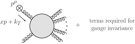
Figure 1: In high energy factorization for forward jets (hybrid factorization [58, 40]) the multigluon amplitude has one incoming momentum off mass shell, with the off-shell propagator projected onto light-like momentum $p^{\mu}$ (typically the momentum of the hadron to which the gluon couples). The momentum of the off-shell leg has only one longitudinal component in the high energy kinematics. Such amplitude is in general not gauge invariant and additional terms are required to define it properly.

In order to apply the embedding method at one-loop level, and in particular to validate the general concept of [57], it is reasonable to start with the simplest one-loop helicity amplitudes. In the on-shell case, these are the amplitudes with all helicities being the same, say ’plus’ (we use the convention that all momenta are outgoing). Such amplitudes vanish at tree level, but are non-zero at loop level. Thus, in the present work, we shall calculate one-loop amplitudes with all-plus helicity gluons and one off-shell gluon, consistent with the gauge invariance and the high energy limit of QCD. Our result will be presented for arbitrary number of gluons $n$. In particular, we find that for $n=3$ our general result coincides with the existing result obtained from Lipatov’s effective action [39].

As a basis for our calculation we shall use the existing one-loop results for $(-+\dots+)$ helicity on-shell amplitudes, where the first pair of particles is either gluon pair or quark-antiquark pair. The particles with helicity $+-$ will provide an auxiliary quark or gluon line, with corresponding external spinors parametrized in a way that – upon taking a proper limit – will guarantee both the high energy kinematics Eq. (1) and the eikonal coupling for the internal off-shell gluon attached to it.

We shall focus on the so-called color ordered amplitudes corresponding to planar diagrams and utilize the spinor helicity method (see [59] for a review). At tree level, the color decomposition of a full gluon amplitude into color ordered amplitudes is

$$\mathcal{M}^{a_{1},\dots,a_{n}}_{\lambda_{1},\dots,\lambda_{n}}\left(k_{1},\dots,k_{n}\right)=\sum_{\textsf{perm.}(2\cdots n)}\,\mathrm{Tr}\left(t^{a_{1}}t^{a_{2}}\dots t^{a_{n}}\right)\,\mathcal{A}\left(1^{(\lambda_{1})},2^{(\lambda_{2})},\dots,n^{(\lambda_{n})}\right)\,,$$ (2)

where $t^{a}$ are color generators, $k_{i}$ is momentum of $i$-th gluon with helicity projection $\lambda_{i}$ and the sum goes over all non-cyclic permutations of the arguments of the trace and the arguments of the color ordered amplitudes $\mathcal{A}$. At one-loop level, additional double trace terms are present. They can be however obtained as linear combinations of the leading trace contributions.

It is known that the on-shell $(\pm+\dots+)$ one-loop amplitudes have rather simple structure, given by a rational function of spinor products. Consider for instance the all-plus on-shell leading trace color ordered amplitude. It has a remarkably simple form for arbitrary number of gluons (conjectured by Z. Bern, G. Chalmers, L. J. Dixon and D. A. Kosower in [60, 61] and demonstrated by G. Mahlon in [62]) :

$$\mathcal{A}_{n}^{(1)}=g_{s}^{n}\sum_{1\leq i<j<k<l\leq n}\frac{\langle ij\rangle[jk]\langle kl\rangle[li]}{\langle 12\rangle\cdots\langle n1\rangle}$$ (3)

Above, the spinor products are defined as

$$\langle ij\rangle=\overline{u}_{-}\left(k_{i}\right)u_{+}\left(k_{j}\right)\qquad[ij]=\overline{u}_{+}\left(k_{i}\right)u_{-}\left(k_{j}\right)\,,$$ (4)

where $u_{\pm}(k)$ are the spinors of helicity $\pm$ for an on-shell momentum $k$. The above result is most easily understood within the unitarity methods (see eg. [63]), or – more generally – the on-shell methods (see [64] for a comprehensive review). The off-shell gauge invariant amplitudes we calculate in the present work inherit the rational structure.

Our paper has the following structure. In the next section, we will describe the embedding method in more detail. Next, in Section 3, we will present the main results for the amplitudes. In Section 4 we recalulate the amplitudes using the embedding method with auxiliary gluon line as a verification of our results. In Section 5 we will investigate the on-shell limit of the obtained off-shell amplitudes. Finally, in Section 6 we shall summarize our work and discuss further perspectives.

2 The method

The method to obtain the off-shell amplitudes we are about to use has been developed in [53]. Here we shall apply it to obtain one loop scattering amplitudes for arbitrary number of positive helicity on-shell gluons and one off-shell gluon with the high energy kinematics Eq. (1) (called also the quasi-multi-Regge kinematics).

Let us briefly recall how the method works. The basic idea is to calculate the amplitude with the off-shell gluon using an on-shell amplitude with an auxiliary quark-antiquark pair, which follows specific kinematics. Ultimately, the auxiliary quark and antiquark spinors are decoupled ensuring gauge invariance of the off-shell amplitude. Schematically, the method can be summarized as (see also Fig. 2)

$$\lim_{\Lambda\to\infty}\left(\frac{x|k_{T}|}{g_{s}\Lambda}\mathcal{A}\left(\bar{q}(k_{1})q(k_{2})\mathcal{X}\right)\right)=\mathcal{A}^{*}\left(g^{*}(k)\mathcal{X}\right)\,,$$ (5)

where $\mathcal{X}$ stands for other on-shell particles involved in the hard scattering process and $\Lambda$ is a real parameter parametrizing momenta of the auxiliary quark pair (see below). The gauge invariant off-shell amplitude is denoted $\mathcal{A}^{*}$. The momenta of the auxiliary quarks are taken to be the following:

$$\begin{split}k_{1}^{\mu}&=\Lambda p^{\mu}+\alpha q^{\mu}+\beta k_{T}^{\mu}\,,\\ k_{2}^{\mu}&=k^{\mu}-k_{1}^{\mu}\,,\end{split}$$ (6)

where

$$\alpha=\frac{-\beta^{2}k_{T}^{2}}{2\Lambda p\cdot q}\quad,\quad\beta=\frac{1}{1+\sqrt{1-x/\Lambda}}$$ (7)

and $q^{\mu}$ is an arbitrary light-like momentum such that $q\cdot k_{T}=0$, $q\cdot p>0$. Note, that $k_{1}^{\mu}$ and $k_{2}^{\mu}$ are light-like and they satisfy $k_{1}^{\mu}+k_{2}^{\mu}=k^{\mu}$, where the latter is the momentum of the off-shell gluon as defined in Eq. (1). In the limit $\Lambda\to\infty$ the coupling of gluons to the quark line becomes eikonal, consistent with the high energy limit. The factor $1/g_{s}$ in Eq. (5) is to correct the power of the coupling, and the factor $x|k_{T}|$ is for the correct matching to $k_{T}$-dependent PDFs in a cross section. In particular, the factor $|k_{T}|$ makes sure the amplitude is finite for $|k_{T}|\to 0$.

$$\leavevmode\hbox to128.81pt{\vbox to62.42pt{\text{[drawing]}}}\hskip 14.22636pt\xrightarrow[\Lambda\to\infty]{}\hskip 17.07182pt\leavevmode\hbox to142.42pt{\vbox to62.42pt{\text{[drawing]}}} q \bar{q} \mathcal{A} \cdots \mathcal{X} g^{*} \mathcal{A}^{*} \cdots \mathcal{X} q \bar{q} \mathcal{A} \cdots \mathcal{X} g^{*} \mathcal{A}^{*} \cdots \mathcal{X}$$

Figure 2: Gauge invariant off-shell amplitudes can be obtained by considering a process with an auxiliary quark-antiquark pair, with momenta parametrized in terms of a parameter $\Lambda$ in such a way, that upon taking the limit $\Lambda\rightarrow\infty$ the coupling to the quark line becomes eikonal and the momentum of the off-shell gluon has the high energy form (see Eq. (1)).

In practice, instead of using the above definitions of $k_{1}^{\mu}$ and $k_{2}^{\mu}$, we will use their expansion in $\Lambda$:

$$\begin{split}k_{1}^{\mu}&=\Lambda p^{\mu}+\left(\frac{1}{2}+\frac{x}{8\Lambda}\right)k_{T}^{\mu}-\frac{k_{T}^{2}}{8\Lambda p\cdot q}q^{\mu}+\mathcal{O}(\Lambda^{-2})\,,\\ k_{2}^{\mu}&=(x-\Lambda)p^{\mu}+\left(\frac{1}{2}-\frac{x}{8\Lambda}\right)k_{T}^{\mu}+\frac{k_{T}^{2}}{8\Lambda p\cdot q}q^{\mu}+\mathcal{O}(\Lambda^{-2})\,.\\ \end{split}$$ (8)

In order to use the helicity method, we need to express $k_{T}^{\mu}$ in terms of spinors. It can be decomposed as follows

$$k_{T}^{\mu}=-\bar{\kappa}e^{\mu}-\bar{\kappa}^{*}e_{*}^{\mu}\,,$$ (9)

with

$$e^{\mu}=\frac{1}{2}\langle p|\gamma^{\mu}|q]\quad,\quad e_{*}^{\mu}=\frac{1}{2}\langle q|\gamma^{\mu}|p]$$ (10)

and

$$\bar{\kappa}=\frac{\kappa}{[pq]}=\frac{\langle q|\not{k}|p]}{2p\cdot q}\quad,\quad\bar{\kappa}^{*}=\frac{\kappa^{*}}{\langle qp\rangle}=\frac{\langle p|\not{k}|q]}{2p\cdot q}\,.$$ (11)

Realize that $k_{T}^{\mu}$ is a four-vector with a negative square, and we have

$$k_{T}^{2}=-\kappa\kappa^{*}~{}.$$ (12)

The spinors of $k_{1}^{\mu}$ and $k_{2}^{\mu}$ can be decomposed into those of $p^{\mu}$ and $q^{\mu}$ following

$$|1\rangle=\sqrt{\Lambda}\,|p\rangle-\frac{\beta\bar{\kappa}^{*}}{\sqrt{\Lambda}}\,|q\rangle\quad ,\quad|1]=\sqrt{\Lambda}\,|p]-\frac{\beta\bar{\kappa}}{\sqrt{\Lambda}}\,|q]$$ (13)

$$|2\rangle=\sqrt{\Lambda-x}\,|p\rangle+\frac{\beta\bar{\kappa}^{*}}{\sqrt{\Lambda}}\,|q\rangle\quad ,\quad|2]=-\sqrt{\Lambda-x}\,|p]-\frac{\beta\bar{\kappa}}{\sqrt{\Lambda}}\,|q]~{}.$$ (14)

Notice that $\sqrt{(\Lambda-x)/\Lambda}\,\beta=1-\beta$. We see that the spinor products

$$\langle 12\rangle=-\kappa^{*}\quad,\quad[12]=-\kappa$$ (15)

are independent of $\Lambda$. Further, the spinors for auxiliary quarks behave for large $\Lambda$ as

$$|1\rangle\to\sqrt{\Lambda}\,|p\rangle\;\;,\;\;|1]\to\sqrt{\Lambda}\,|p]\;\;,\;\;|2\rangle\to\sqrt{\Lambda}\,|p\rangle\;\;,\;\;|2]\to-\sqrt{\Lambda}\,|p]\;\;.$$ (16)

In what follows, we shall call the above kinematics (together with taking the limit $\Lambda\to\infty$) the “$\Lambda$ prescription”. Applying it to an amplitude with auxiliary partons gives the gauge invariant off-shell amplitude.

Alternatively, the “embedding” method described above can be used with an auxiliary gluon line, instead of the quark line. Indeed, the color decomposition for $(n-2)$-gluon amplitude with a quark-antiquark pair is given by

$$\mathcal{M}^{ij\hskip 11.45277pta_{3},\dots,a_{n}}_{\lambda_{1},\lambda_{2},\lambda_{3},\dots,\lambda_{n}}\left(k_{1},\dots,k_{n}\right)=\sum_{\textsf{perm.}(3\cdots n)}\,\left(t^{a_{3}}\cdots t^{a_{n}}\right)_{ij}\,\mathcal{A}\left(q^{(\lambda_{1})},\bar{q}^{(\lambda_{2})},3^{(\lambda_{3})},\dots,n^{(\lambda_{n})}\right)\,,$$ (17)

and can be projected onto $(n-1)$-gluon amplitude by a contraction with $(t^{a_{*}})_{ji}$, where $a_{*}$ represents the color index of the off-shell gluon. Now, for an auxiliary gluon pair instead of a quark one, one simply needs to select only those permutations in Eq. (2) that retains the order of gluons $1$ and $2$ and substitute $t^{a_{1}}t^{a_{2}}\to t^{a_{*}}$. At one loop, the color decompositions get more complicated and are given by Eq. (1) in [65] and Eq. (2.4-5) in [66] respectively. One can however easily see that the same procedure goes through to extract a single gluon color from a pair of colors. In [57] it has been shown that at tree level, the partial amplitudes obtained using different pairs of auxiliary partons are identical. We will see here that the same holds at one loop for the all-plus amplitudes.

3 All-plus off-shell gauge invariant amplitudes at NLO

In this section we present our results for one loop amplitudes for one off-shell gluon and $n-1$ on-shell positive helicity gluons. We begin with several low multiplicity examples, starting with the simplest cases: $n=3$ (the vertex), $n=4$ and $n=5$. Then, we will turn to a general result for arbitrary $n$. For each case, we first present the known amplitude with auxiliary quarks. Then, we apply the $\Lambda$ prescription to it and give the result for the off-shell amplitude.

3.1 3-point vertex

We first consider the 3-point vertex with one off-shell gluon and two positive helicity on-shell gluons at one loop. Such vertex has been calculated for arbitrary helicity projection in [39] from the Lipatov’s effective action.

In order to calculate it from the $\Lambda$ prescription, we need the 4-point amplitude for quark, anti-quark and two gluons. At one loop it has the following form [66] :

$$\mathcal{A}_{4}^{(1)}(1_{\bar{q}}^{-},2_{q}^{+},3^{+},4^{+})=-\frac{ig_{s}^{4}}{16\pi^{2}}\left[\frac{1}{2}\left(1+\frac{1}{N_{c}^{2}}\right)+\frac{1}{3}\left(1+\frac{n_{s}-n_{f}}{N_{c}}\right)\frac{s_{23}}{s_{12}}\right]\frac{\langle 12\rangle[24]}{\langle 23\rangle\langle 34\rangle}\,,$$ (18)

where $n_{f}$ accounts for the number of Weyl fermions circulating in the loop, $n_{s}$ the number of complex scalars and

$$\forall i,j=1,\dots,n,\ s_{ij}=2k_{i}\cdot k_{j}=\langle ij\rangle[ji]\text{ (in this section, }n=4\text{)}.$$ (19)

Applying the $\Lambda$ prescription we get:

$$\begin{split}\mathcal{A}_{3}^{*(1)}(g^{*},3^{+},4^{+})&=-\frac{ig_{s}^{3}}{24\pi^{2}}\left(1+\frac{n_{s}-n_{f}}{N_{c}}\right)x|k_{T}|\frac{p\cdot k_{3}}{k_{T}^{2}}\frac{\kappa^{*}[p4]}{\langle p3\rangle\langle 34\rangle}\\ &=-\frac{ig_{s}^{3}}{24\pi^{2}}\left(1+\frac{n_{s}-n_{f}}{N_{c}}\right)\frac{x|k_{T}|}{\kappa^{2}}p\cdot k_{3}\frac{[p3][p4]}{\langle p3\rangle\langle p4\rangle},\end{split}$$ (20)

where we used that $k_{T}^{2}=-\kappa\kappa^{*}$, $\kappa=\langle 4|k/|p]/\langle 4p\rangle$ and $k^{\mu}=-k_{3}^{\mu}-k_{4}^{\mu}$. We checked that for $n_{s}=0$ the above result agrees with the one of [67, 39], up to an overall constant and a factor $xE/|k_{T}|$, where $E$ is the energy component of $p^{\mu}$. This difference is due to the fact that in the mentioned publications vertices rather than amplitudes are calculated (see also the comparisons at tree-level in [53]).

3.2 4-point amplitude

The 5-leg amplitude with auxiliary quark pair is given by [66] :

$$\begin{split}\mathcal{A}_{5}^{(1)}(1_{\bar{q}}^{-},2_{q}^{+},3^{+},4^{+},5^{+})=&-\frac{ig_{s}^{5}}{32\pi^{2}}\left(1+\frac{1}{N_{c}^{2}}\right)\frac{\langle 12\rangle[23]\langle 31\rangle+\langle 14\rangle[45]\langle 51\rangle}{\langle 23\rangle\langle 34\rangle\langle 45\rangle\langle 51\rangle}\\ -\frac{ig_{s}^{5}}{48\pi^{2}}\left(1+\frac{n_{s}-n_{f}}{N_{c}}\right)&\bigg{(}\frac{\langle 13\rangle[34]\langle 41\rangle^{2}}{\langle 12\rangle\langle 34\rangle^{2}\langle 45\rangle\langle 51\rangle}+\frac{\langle 14\rangle\langle 24\rangle[45]\langle 51\rangle}{\langle 12\rangle\langle 23\rangle\langle 34\rangle\langle 45\rangle^{2}}+\frac{[23][25]}{[12]\langle 34\rangle\langle 45\rangle}\bigg{)}.\end{split}$$ (21)

Applying the $\Lambda$ prescription we find that the first term is of the order $\Lambda^{-1}$ and thus vanishes. Further calculation leads to the following result

$$\begin{split}\mathcal{A}_{4}^{*(1)}(g^{*},3^{+},4^{+},5^{+})=&-\frac{ig_{s}^{4}}{48\pi^{2}}\frac{x|k_{T}|\left(1+\frac{n_{s}-n_{f}}{N_{c}}\right)}{\kappa^{*}\langle p3\rangle\langle 34\rangle\langle 45\rangle\langle 5p\rangle}\\ &\times\bigg{[}\langle p3\rangle^{2}\langle p4\rangle^{2}\frac{[34]}{\langle 34\rangle}+\langle p4\rangle^{2}\langle p5\rangle^{2}\frac{[45]}{\langle 45\rangle}-\frac{\kappa^{*}}{\kappa}s_{p3}s_{p5}\bigg{]}\,.\end{split}$$ (22)

3.3 5-point amplitude

The amplitude with the auxiliary quark pair is given by [68] :

$$\begin{split}\mathcal{A}_{6}^{(1)}(1_{\bar{q}}^{-},2_{q}^{+},3^{+},4^{+},5^{+},6^{+})=&\frac{ig_{s}^{6}}{32\pi^{2}}\left(1+\frac{1}{N_{c}^{2}}\right)\frac{\sum_{l=3}^{5}{\langle 1|\not{K}_{2\dots l}\not{k}_{l}}|1]}{\langle 23\rangle\langle 34\rangle\langle 45\rangle\langle 56\rangle\langle 61\rangle}\\ +\frac{ig_{s}^{6}}{48\pi^{2}}\left(1+\frac{n_{s}-n_{f}}{N_{c}}\right)\Bigg{[}&\frac{\langle 14\rangle\langle 1|(2+3)(3+4)|1\rangle}{\langle 12\rangle\langle 34\rangle^{2}\langle 45\rangle\langle 56\rangle\langle 61\rangle}+\frac{\langle 24\rangle\langle 15\rangle\langle 1|(4+5)(5+6)|1\rangle}{\langle 12\rangle\langle 23\rangle\langle 34\rangle\langle 45\rangle^{2}\langle 56\rangle\langle 61\rangle}\\ &-\frac{\langle 25\rangle\langle 1|56|1\rangle}{\langle 12\rangle\langle 23\rangle\langle 34\rangle\langle 45\rangle\langle 56\rangle^{2}}+\frac{\langle 1|3+4|2]^{2}}{\langle 34\rangle^{2}\langle 56\rangle\langle 61\rangle\langle 5|3+4|2]}\\ &+\frac{\langle 2|4+5|6]\langle 1|4+5|6]^{2}}{\langle 12\rangle\langle 23\rangle\langle 45\rangle^{2}\langle 3|4+5|6]s_{456}}\\ &-\frac{[26]^{2}[2|(3+4)(4+5)(3+4)(4+5)|6]}{[12]\langle 34\rangle\langle 45\rangle\langle 5|3+4|2]\langle 3|4+5|6]s_{345}}\Bigg{]}\,,\end{split}$$ (23)

where we defined

$$\not{K}_{a\cdots b}=\sum_{i=a}^{b}\not{k}_{i}\,,$$ (24)

$$s_{ijk}=\left(k_{i}+k_{j}+k_{k}\right)^{2}\,,$$ (25)

and used

$$\langle a|(i+j)|b]=\langle ai\rangle[ib]+\langle aj\rangle[jb]$$ (26)

$$\langle a|(i+j)(k+l)|b\rangle=\langle ai\rangle[i|(k+l)|b\rangle+\langle aj\rangle[j|(k+l)|b\rangle\,.$$ (27)

Above $a,b,i,j,k,l=1,\dots n$, where $n=6$ in the present section.

After we apply the $\Lambda$ prescription we find that the term with the factor $\left(1+\frac{1}{N_{c}^{2}}\right)$ vanishes leading to

$$\begin{split}\mathcal{A}_{5}^{*(1)}(g^{*},3^{+},&4^{+},5^{+},6^{+})=\left(1+\frac{n_{s}-n_{f}}{N_{c}}\right)\times\\ \times\frac{ig_{s}^{5}x|k_{T}|}{48\pi^{2}}\Bigg{[}&\frac{\langle p4\rangle(\kappa^{*}[p|3+4|p\rangle+\langle p3\rangle[34]\langle 4p\rangle)}{\kappa^{*}\langle 34\rangle^{2}\langle 45\rangle\langle 56\rangle\langle 6p\rangle}+\frac{\langle p4\rangle\langle p5\rangle\langle p|(4+5)(5+6)|p\rangle}{\kappa^{*}\langle p3\rangle\langle 34\rangle\langle 45\rangle^{2}\langle 56\rangle\langle 6p\rangle}\\ &-\frac{\langle p5\rangle\langle p|56|p\rangle}{\kappa^{*}\langle p3\rangle\langle 34\rangle\langle 45\rangle\langle 56\rangle^{2}}+\frac{\langle p|3+4|p]^{2}}{\langle 34\rangle^{2}\langle 56\rangle\langle 6p\rangle\langle 5|3+4|p]}\\ &+\frac{\langle p|4+5|6]^{3}}{\kappa^{*}\langle p3\rangle\langle 45\rangle^{2}\langle 3|4+5|6]s_{456}}-\frac{[p6]^{2}[p|(3+4)(4+5)(3+4)(4+5)|6]}{\kappa\langle 34\rangle\langle 45\rangle\langle 5|3+4|p]\langle 3|4+5|6]s_{345}}\Bigg{]}\,.\end{split}$$ (28)

3.4 $n$-point amplitude

Finally, in the following section we shall derive the general expression for one-loop amplitude for one off-shell gluon and $n-1$ on-shell gluons with all helicities positive. To this end, we need the one loop amplitude for a quark-antiquark pair and $n-1$ positive helicity gluons. A suitable expression has been derived in [68]. It reads

$$\begin{split}\mathcal{A}_{n+1}^{(1)}(1_{\bar{q}}^{-},2_{q}^{+},3^{+},\cdots,(n+1)^{+})=&\frac{ig_{s}^{n+1}}{32\pi^{2}}\left(1+\frac{1}{N_{c}^{2}}\right)\frac{\sum_{l=3}^{n}\langle 1|\not{K}_{2\cdots l}\not{k}_{l}|1\rangle}{\langle 23\rangle\cdots\langle(n+1)1\rangle}\\ +&\frac{ig_{s}^{n+1}}{48\pi^{2}}\left(1+\frac{n_{s}-n_{f}}{N_{c}}\right)\frac{S_{1}+S_{2}}{\langle 12\rangle\langle 23\rangle\cdots\langle(n+1)1\rangle}\,,\end{split}$$ (29)

with

$$\begin{split}S_{1}=&\sum_{j=3}^{n}\frac{\langle 2j\rangle\langle 1(j+1)\rangle\langle 1|\not{K}_{j,j+1}\not{K}_{(j+1)\cdots(n+1)}|1\rangle}{\langle j(j+1)\rangle}\,,\\ S_{2}=&\sum_{j=3}^{n-1}\sum_{l=j+1}^{n}\frac{\langle 1|\not{K}_{j\cdots l}\not{K}_{(l+1)\cdots(n+1)}|1\rangle^{2}\langle 2|\not{K}_{j\cdots l}\not{K}_{(l+1)\cdots(n+1)}|1\rangle}{\langle 1|\not{K}_{(l+1)\cdots(n+1)}\not{K}_{j\cdots l}|(j-1)\rangle\langle 1|\not{K}_{(l+1)\cdots(n+1)}\not{K}_{j\cdots l}|j\rangle}\\ &\hskip 31.2982pt\times\frac{\langle(j-1)j\rangle\langle l(l+1)\rangle\langle 1|\not{K}_{2\cdots(j-1)}[\mathcal{F}(j,l)]^{2}\not{K}_{(l+1)\cdots(n+1)}|1\rangle}{\langle 1|\not{K}_{2\cdots(j-1)}\not{K}_{j\cdots l}|l\rangle\langle 1|\not{K}_{2\cdots(j-1)}\not{K}_{j\cdots l}|(l+1)\rangle s_{j\cdots l}}\,,\end{split}$$ (30)

where

$$\mathcal{F}(j,l)=\sum_{i=j}^{l-1}\sum_{m=i+1}^{l}\not{k}_{i}\not{k}_{m}\,.$$ (31)

After applying the $\Lambda$ prescription we find that the term with the factor $\left(1+\frac{1}{N_{c}^{2}}\right)$ is of the order $\Lambda^{-1}$, whereas the other term is of order $1$ and is the one contributing to the off-shell amplitude. Eventually, we obtain the following expression for the off-shell amplitude:

$$\mathcal{A}_{n}^{*(1)}(g^{*},3^{+},\cdots,(n+1)^{+})=\frac{ig_{s}^{n}x|k_{T}|}{48\pi^{2}}\left(1+\frac{n_{s}-n_{f}}{N_{c}}\right)\frac{U^{*}_{1}+U^{*}_{2}+U^{*}_{3}}{\kappa^{*}\langle p3\rangle\langle 34\rangle\cdots\langle np\rangle}\,,$$ (32)

with

$$\begin{split}U^{*}_{1}=&\sum_{j=3}^{n}\frac{\langle pj\rangle\langle p(j+1)\rangle\langle p|\not{K}_{j,j+1}\not{K}_{(j+1)\cdots(n+1)}|p\rangle}{\langle j(j+1)\rangle}\,,\\ U^{*}_{2}=&\sum_{j=4}^{n-1}\sum_{l=j+1}^{n}\frac{\langle p|\not{K}_{j\cdots l}\not{K}_{(l+1)\cdots(n+1)}|p\rangle^{3}}{\langle p|\not{K}_{(l+1)\cdots(n+1)}\not{K}_{j\cdots l}|(j-1)\rangle\langle p|\not{K}_{(l+1)\cdots(n+1)}\not{K}_{j\cdots l}|j\rangle}\\ &\hskip 31.2982pt\times\frac{\langle(j-1)j\rangle\langle l(l+1)\rangle\langle p|\not{K}^{\prime}_{3\cdots(j-1)}[\mathcal{F}(j,l)]^{2}\not{K}_{(l+1)\cdots(n+1)}|p\rangle}{\langle p|\not{K}_{3\cdots(j-1)}\not{K}_{j\cdots l}|l\rangle\langle p|\not{K}_{3\cdots(j-1)}\not{K}_{j\cdots l}|(l+1)\rangle s_{j\cdots l}}\,,\\ U^{*}_{3}=&\sum_{l=4}^{n}\frac{\langle p|\not{K}_{3\cdots l}\not{K}_{(l+1)\cdots(n+1)}|p\rangle^{3}}{\langle p|\not{K}_{(l+1)\cdots(n+1)}\not{K}_{3\cdots l}|p\rangle\langle p|\not{K}_{(l+1)\cdots(n+1)}\not{K}_{3\cdots l}|3\rangle}\\ &\hskip 31.2982pt\times\frac{\langle p3\rangle\langle l(l+1)\rangle[p|[\mathcal{F}(3,l)]^{2}\not{K}_{(l+1)\cdots(n+1)}|p\rangle}{\kappa^{*}[p|\not{K}_{3\cdots l}|l\rangle[p|\not{K}_{3\cdots l}|(l+1)\rangle s_{3\cdots l}}\,.\end{split}$$ (33)

It can be readily checked that the above expression recovers the amplitudes calculated previously for $n=3,4,5$ in an independent way.

4 Verification with auxiliary gluon pair

In the following section we shall verify the off-shell gauge invariant amplitudes we obtained in the previous section by applying the $\Lambda$ prescription to the corresponding $n$-point amplitude with an auxiliary gluon pair, instead of the auxiliary quark pair. This will provide a nontrivial check of our calculations.

4.1 3-point amplitude

The 4-point one loop amplitude for one negative helicity gluon and three positive helicity gluons is given by [66]

$$\mathcal{A}_{4}^{(1)}(1^{-},2^{+},3^{+},4^{+})=\frac{ig_{s}^{4}}{48\pi^{2}}\left(1+\frac{n_{s}-n_{f}}{N_{c}}\right)\frac{\langle 24\rangle[24]^{3}}{[12]\langle 23\rangle\langle 34\rangle[41]}\,.$$ (34)

After applying the $\Lambda$ prescription we indeed find that it leads to the same result as before:

$$\mathcal{A}_{3}^{*(1)}(g^{*},3^{+},4^{+})=-\frac{ig_{s}^{3}x|k_{T}|}{24\pi^{2}}\left(1+\frac{n_{s}-n_{f}}{N_{c}}\right)\frac{p\cdot k_{3}}{k_{T}^{2}}\frac{\kappa^{*}[p4]}{\langle p3\rangle\langle 34\rangle}\,,$$ (35)

where we used $p\cdot k_{3}=-p\cdot k_{4}$ since $0=p\cdot k=p\cdot(-k_{3}-k_{4})$.

4.2 4-point amplitude

The 5-point on-shell gluon amplitude we need is given by [65]

$$\begin{split}\mathcal{A}_{5}^{(1)}(1^{-},2^{+},3^{+},4^{+},5^{+})=&\frac{ig_{s}^{5}}{48\pi^{2}}\frac{\left(1+\frac{n_{s}-n_{f}}{N_{c}}\right)}{[12]\langle 23\rangle\langle 34\rangle\langle 45\rangle[51]}\times\bigg{[}(s_{23}+s_{34}+s_{45})[25]^{2}\\ -[24]\langle 43\rangle[35][25]-\frac{[12][15]}{\langle 12\rangle\langle 15\rangle}&\left(\langle 12\rangle^{2}\langle 13\rangle^{2}\frac{[23]}{\langle 23\rangle}+\langle 13\rangle^{2}\langle 14\rangle^{2}\frac{[34]}{\langle 34\rangle}+\langle 14\rangle^{2}\langle 15\rangle^{2}\frac{[45]}{\langle 45\rangle}\right)\bigg{]}\,.\end{split}$$ (36)

Applying the same procedure as before leads to the following off-shell amplitude

$$\begin{split}\mathcal{A}_{4}^{*(1)}(g^{*},3^{+},4^{+},5^{+})=&\frac{ig_{s}^{4}}{48\pi^{2}}\frac{x|k_{T}|\left(1+\frac{n_{s}-n_{f}}{N_{c}}\right)}{\kappa^{*}\langle p3\rangle\langle 34\rangle\langle 45\rangle[5p]}\times\bigg{[}s_{p3}[p5]^{2}\\ -\frac{\kappa[p5]}{\kappa^{*}\langle p5\rangle}&\left(\langle p3\rangle^{2}\langle p4\rangle^{2}\frac{[34]}{\langle 34\rangle}+\langle p4\rangle^{2}\langle p5\rangle^{2}\frac{[45]}{\langle 45\rangle}\right)\bigg{]}\,,\end{split}$$ (37)

which turns out to be equal to Eq. (22).

4.3 5-point amplitude

In order to derive 5-point off-shell amplitude we use the following 6-point on-shell one loop amplitude [68] :

$$\begin{split}\mathcal{A}_{6}^{(1)}(1^{-},2^{+},3^{+},4^{+},&5^{+},6^{+})=\frac{ig_{s}^{6}}{48\pi^{2}}\left(1+\frac{n_{s}-n_{f}}{N_{c}}\right)\times\\ \times\Bigg{[}&\frac{\langle 1|2+3|6]^{3}}{\langle 12\rangle\langle 23\rangle\langle 45\rangle^{2}s_{123}\langle 3|1+2|6]}+\frac{\langle 1|3+4|2]^{3}}{\langle 34\rangle^{2}\langle 56\rangle\langle 61\rangle s_{234}\langle 5|3+4|2]}\\ &+\frac{[26]^{3}}{[12][61]s_{345}}\left(\frac{[23][34]}{\langle 45\rangle\langle 5|3+4|2]}-\frac{[45][56]}{\langle 34\rangle\langle 3|1+2|6]}+\frac{[35]}{\langle 34\rangle\langle 45\rangle}\right)\\ &-\frac{\langle 13\rangle^{3}[23]\langle 24\rangle}{\langle 23\rangle^{2}\langle 34\rangle^{2}\langle 45\rangle\langle 56\rangle\langle 61\rangle}+\frac{\langle 15\rangle^{3}\langle 46\rangle[56]}{\langle 12\rangle\langle 23\rangle\langle 34\rangle\langle 45\rangle^{2}\langle 56\rangle^{2}}\\ &-\frac{\langle 14\rangle^{3}\langle 35\rangle\langle 1|2+3|4]}{\langle 12\rangle\langle 23\rangle\langle 34\rangle^{2}\langle 45\rangle^{2}\langle 56\rangle\langle 61\rangle}\Bigg{]}\,.\end{split}$$ (38)

Applying the $\Lambda$ prescription to the above on-shell result gives

$$\begin{split}\mathcal{A}_{5}^{*(1)}(g^{*},3^{+},4^{+},5^{+},6^{+})&=\frac{ig_{s}^{5}x|k_{T}|}{48\pi^{2}}\left(1+\frac{n_{s}-n_{f}}{N_{c}}\right)\times\\ \times\Bigg{[}&\frac{(\kappa^{*}[p6]+\langle p3\rangle[36])^{3}}{\kappa^{*}\langle p3\rangle\langle 45\rangle^{2}s_{k3}\langle 3|k|6]}+\frac{\langle p|3+4|p]^{3}}{\langle 34\rangle^{2}\langle 56\rangle\langle 6p\rangle(s_{p3}+s_{p4})\langle 5|3+4|p]}\\ &+\frac{[p6]^{2}}{\kappa^{*}s_{345}}\left(\frac{[p3][34]}{\langle 45\rangle\langle 5|3+4|p]}-\frac{[45][56]}{\langle 34\rangle\langle 3|k|6]}+\frac{[35]}{\langle 34\rangle\langle 45\rangle}\right)\\ &-\frac{\langle p3\rangle[p3]\langle p4\rangle}{\langle 34\rangle^{2}\langle 45\rangle\langle 56\rangle\langle 6p\rangle}+\frac{\langle p5\rangle^{3}\langle 46\rangle[56]}{\kappa^{*}\langle p3\rangle\langle 34\rangle\langle 45\rangle^{2}\langle 56\rangle^{2}}\\ &-\frac{\langle p4\rangle^{3}\langle 35\rangle(\kappa^{*}[p4]+\langle p3\rangle[34])}{\kappa^{*}\langle p3\rangle\langle 34\rangle^{2}\langle 45\rangle^{2}\langle 56\rangle\langle 6p\rangle}\Bigg{]}\,.\end{split}$$ (39)

This amplitude turns out to be equal to the one obtained with auxiliary quark line, Eq. (23). The comparison is detailed in Appendix A.

4.4 $n$-point amplitude

For the general case of $n$-point amplitude, the on-shell gluonic amplitude is taken from [68]

$$\mathcal{A}_{n+1}^{(1)}(1^{-},2^{+},3^{+},\cdots,(n+1)^{+})=\frac{ig_{s}^{n+1}}{48\pi^{2}}\left(1+\frac{n_{s}-n_{f}}{N_{c}}\right)\frac{T_{1}+T_{2}}{\langle 12\rangle\langle 23\rangle\cdots\langle n1\rangle}\,,$$ (40)

with

$$\begin{split}T_{1}=&\sum_{j=2}^{n}\frac{\langle 1j\rangle\langle 1(j+1)\rangle\langle 1|\not{K}_{j,j+1}\not{K}_{(j+1)\cdots(n+1)}|1\rangle}{\langle j(j+1)\rangle}\,,\\ T_{2}=&\sum_{j=3}^{n-1}\sum_{l=j+1}^{n}\frac{\langle 1|\not{K}_{j\cdots l}\not{K}_{(l+1)\cdots(n+1)}|1\rangle^{3}}{\langle 1|\not{K}_{(l+1)\cdots(n+1)}\not{K}_{j\cdots l}|(j-1)\rangle\langle 1|\not{K}_{(l+1)\cdots(n+1)}\not{K}_{j\cdots l}|j\rangle}\\ &\hskip 36.98866pt\times\frac{\langle(j-1)j\rangle\langle l(l+1)\rangle\langle 1|\not{K}_{2\cdots(j-1)}[\mathcal{F}(j,l)]^{2}\not{K}_{(l+1)\cdots(n+1)}|1\rangle}{\langle 1|\not{K}_{2\cdots(j-1)}\not{K}_{j\cdots l}|l\rangle\langle 1|\not{K}_{2\cdots(j-1)}\not{K}_{j\cdots l}|(l+1)\rangle s_{j\cdots l}}\,.\end{split}$$ (41)

Applying the $\Lambda$ prescription to $T_{2}$ gives the same result as for $S_{2}$ in Eq. (30). It turns out that $T_{1}$ is equal to $S_{1}$ within the $\Lambda$ description once you realize that the first term in the sum over $j$ in $T_{1}$ is of the order $\Lambda^{-1}$. In the end, applying the $\Lambda$ prescription to $\bar{q}^{-}q^{+}g^{+}\cdots g^{+}$ or $g^{-}g^{+}g^{+}\cdots g^{+}$ gives the same expression, given by Eq. (32).

5 On-shell limit

Now, that we have obtained the expression for $\mathcal{A}_{n}^{*(1)}(g^{*},3^{+},\cdots,(n+1)^{+})$, we should verify that in the on-shell limit, i.e. when $|k_{T}|\to 0$, we obtain the one loop on-shell amplitude with the first gluon having the momentum $xp^{\mu}$. We expect that the limit consists of the sum of the amplitudes for which the, now on-shell, gluon has either negative or positive helicity. For tree-level amplitudes, this can be understood as follows. Firstly, at the on-shell limit, the contributions to the amplitude that dominate have a propagator with denominator $k_{T}^{2}=-\kappa\kappa^{*}$, and have exactly the form of the first term in Fig. 1. More precisely, they have the form

$$\sqrt{2}\,p^{\mu}\,\frac{x|k_{T}|}{\kappa\kappa^{*}}\,J_{\mu}$$ (42)

where we use the planar Feynman rules as in Eq. (10) of [69], where $J_{\mu}$ represents the off-shell current, and where we included the factor $x|k_{T}|$ from the $\Lambda$-prescription. Using the current conservation $k\cdot J=0$, we can see that projecting on $p^{\mu}$ is equivalent to projecting on $-k_{T}^{\mu}/x$. Secondly, using Eq. (9) to Eq. (11), we see that

$$k_{T}^{\mu}=-\frac{\kappa}{\sqrt{2}}\,\varepsilon_{-}^{\mu}(p,q)-\frac{\kappa^{*}}{\sqrt{2}}\,\varepsilon_{+}^{\mu}(p,q)\,,$$ (43)

with polarization vectors

$$\varepsilon_{-}^{\mu}(p,q)=\frac{\langle p|\gamma^{\mu}|q]}{\sqrt{2}\,[pq]}\quad,\quad\varepsilon_{+}^{\mu}(p,q)=\frac{\langle q|\gamma^{\mu}|p]}{\sqrt{2}\,\langle qp\rangle}~{}.$$ (44)

Thus we find

$$\lim_{|k_{T}|\to 0}{\mathcal{A}_{n}^{*(0)}(g^{*}\mathcal{X})}=\frac{|k_{T}|}{\kappa^{*}}\mathcal{A}_{n}^{(0)}(g^{-}\mathcal{X})+\frac{|k_{T}|}{\kappa}\mathcal{A}_{n}^{(0)}(g^{+}\mathcal{X})~{},$$ (45)

where $|k_{T}|/\kappa^{*}=e^{\mathrm{i}\phi}$ for some angle $\phi$, and $|k_{T}|/\kappa$ its complex conjugate, and where $\mathcal{A}_{n}^{(0)}(g^{\pm}\mathcal{X})=\varepsilon_{\pm}\cdot J$. In [69] it is explained how such a coherent sum of amplitudes becomes an incoherent sum of squared amplitudes in a cross section.

When taking the on-shell limits in expressions consisting of spinor products and invariants involving the momentum $p^{\mu}$, the final step is to interpret this momentum as the momentum of the now on-shell gluon, divided by $x$. Since the tree amplitudes are homogeneous in $p^{\mu}$ of degree $1$, this results in the overall factor $1/x$ equivalent to the one coming from changing the projector $p^{\mu}\to-k_{T}^{\mu}/x$ above. The off-shell one-loop all-plus amplitudes can easily be checked to be homogeneous in $p^{\mu}$ of degree $1$ too, and the same factor $1/x$ will show up to cancel the factor $x$ from the $\Lambda$-prescription.

We now verify that the same limit appears for the one-loop $n$-point all-plus amplitudes we obtained in Section 3.4. One can notice that $U^{*}_{1}\xrightarrow[|k_{T}|\to 0]{}T^{1}$ and $U^{*}_{2}\xrightarrow[|k_{T}|\to 0]{}T^{2}$, which implies

$$\begin{split}\lim_{|k_{T}|\to 0}{\mathcal{A}_{n}^{*(1)}(g^{*},3^{+},\cdots,(n+1)^{+})}=&\frac{|k_{T}|}{\kappa^{*}}\mathcal{A}_{n}^{(1)}(xp^{-},3^{+},\cdots,(n+1)^{+})\\ &+\frac{ig_{s}^{n}x}{48\pi^{2}}\frac{\lim_{k_{T}\to 0}{\left(U^{*}_{3}|k_{T}|/\kappa^{*}\right)}}{\langle p3\rangle\langle 34\rangle\cdots\langle(n+1)p\rangle}\,.\end{split}$$ (46)

So we already have the contribution from the amplitude with negative helicity gluon (the first term in the expression above). We now need to show that the second term is actually the contribution from the amplitude with a positive helicity gluon, i.e.

$$\mathcal{A}_{n}^{(1)}(1^{+},\cdots,n^{+})=\frac{ig^{n}}{48\pi^{2}}\left(1+\frac{n_{s}-n_{f}}{N_{c}}\right)\sum_{1\leq i<j<k<l\leq n}\frac{\langle ij\rangle[jk]\langle kl\rangle[li]}{\langle 12\rangle\cdots\langle n1\rangle}.$$ (47)

To this end, we have to manipulate on the expression $U^{*}_{3}$. One can show that

$$\begin{split}U^{*}_{3}\xrightarrow[|k_{T}|\to 0]{}\frac{\kappa^{*}}{\kappa[p(n+1)]}[p|[\mathcal{F}(3,n)]^{2}|(n+1)]=&\frac{\kappa^{*}}{\kappa}\sum_{3\leq i<j<k<l\leq(n+1)}\langle ij\rangle[jk]\langle kl\rangle[li]\\ &+\frac{\kappa^{*}}{\kappa}\sum_{3\leq j<k<l\leq(n+1)}\langle pj\rangle[jk]\langle kl\rangle[lp]\,.\end{split}$$ (48)

Inserting this into Eq. (46) leads to

$$\begin{split}\lim_{k_{T}\to 0}{\mathcal{A}_{n}^{*(1)}(g^{*},3^{+},\cdots,(n+1)^{+})}=&\frac{|k_{T}|}{\kappa^{*}}\mathcal{A}_{n}^{(1)}(xp^{-},3^{+},\cdots,(n+1)^{+})\\ &+\frac{|k_{T}|}{\kappa}\mathcal{A}_{n}^{(1)}(xp^{+},3^{+},\cdots,(n+1)^{+})\,.\end{split}$$ (49)

More details on the above rather non-trivial calculation are given in Appendix B. This is exactly what we expect from the on-shell limit of an off-shell amplitude, based on the limit for tree-level amplitudes (Eq. (45)): a superposition of on-shell amplitudes, where the off-shell gluon is replaced by a gluon with a positive and negative helicity.

6 Summary

In this paper we have calculated expressions for amplitudes in high energy factorization with one off-shell gluon and any number of plus-helicity gluons at one loop level. We also obtained expressions for specific cases: 3, 4 and 5 point amplitudes. To obtain these results we used the embedding method developed in [53, 57]. The method relies on identifying pair of on-shell partons as auxiliary lines which can be decoupled in high energy limit, leaving gauge invariant off-shell amplitude with proper high energy kinematics. We find agreement with the existing calculation for the 3-point vertex with a Reggeized gluon in [39]. Furthermore we explicitly demonstrated that we obtain the correct on-shell limit for all calculated amplitudes. Thus, we conclude that the embedding method works at the one-loop level, at least for amplitudes with same helicities.

Our future plans involve calculation of other QCD amplitudes and, in particular, addressing also the real corrections. The ultimate goal is to automatize the NLO calculations in $k_{T}$-factorization as well as the small-$x$ improved TMD factorization (ITMD) [70, 71].

Appendix A 5-point amplitude – detailed calculation

In order to compare the off-shell gauge invariant 5-point amplitude obtained from the auxiliary quark line $\bar{q}^{-}q^{+}g^{+}g^{+}g^{+}g^{+}$ to the one obtained from the auxiliary gluon line $g^{-}g^{+}g^{+}g^{+}g^{+}g^{+}$, we will rewrite both expressions. Let’s first rewrite the first term of the amplitude with auxiliary quarks (before applying the $\Lambda$ prescription, see Eq. (23))

$$\begin{split}\frac{\langle 14\rangle\langle 1|(2+3)(3+4)|1\rangle}{\langle 12\rangle\langle 34\rangle^{2}\langle 45\rangle\langle 56\rangle\langle 61\rangle}&=\frac{\langle 14\rangle(\langle 12\rangle[23]\langle 31\rangle+\langle 1|2+3|4]\langle 41\rangle)}{\langle 12\rangle\langle 34\rangle^{2}\langle 45\rangle\langle 56\rangle\langle 61\rangle}\\ &=-\frac{\langle 14\rangle[23]\langle 13\rangle}{\langle 34\rangle^{2}\langle 45\rangle\langle 56\rangle\langle 61\rangle}+\frac{\langle 23\rangle\langle 45\rangle\langle 14\rangle^{2}\langle 1|5+6|4]}{\langle 12\rangle\langle 23\rangle\langle 34\rangle^{2}\langle 45\rangle^{2}\langle 56\rangle\langle 61\rangle}\\ &=-\frac{\langle 14\rangle[23]\langle 13\rangle}{\langle 34\rangle^{2}\langle 45\rangle\langle 56\rangle\langle 61\rangle}+\frac{\langle 24\rangle\langle 35\rangle\langle 14\rangle^{2}\langle 1|5+6|4]}{\langle 12\rangle\langle 23\rangle\langle 34\rangle^{2}\langle 45\rangle^{2}\langle 56\rangle\langle 61\rangle}\\ &-\frac{\langle 25\rangle\langle 14\rangle^{2}\langle 1|5+6|4]}{\langle 12\rangle\langle 23\rangle\langle 34\rangle\langle 45\rangle^{2}\langle 56\rangle\langle 61\rangle}\,.\\ \end{split}$$ (50)

Above, we have used the momentum conservation to write $\langle 1|2+3|4]=-\langle 1|5+6|4]$ and the Schouten identity: $\langle 23\rangle\langle 45\rangle=\langle 24\rangle\langle 35\rangle+\langle 25\rangle\langle 43\rangle$. It leads to

$$\begin{split}&\mathcal{A}_{5}^{(1)}(g^{*},3^{+},4^{+},5^{+},6^{+})\\ &=\frac{ig^{5}x|k_{T}|}{48\pi^{2}}\Bigg{[}-\frac{\langle p4\rangle[p3]\langle p3\rangle}{\langle 34\rangle^{2}\langle 45\rangle\langle 56\rangle\langle 6p\rangle}+\frac{\langle 35\rangle\langle p4\rangle^{3}\langle p|5+6|4]}{\kappa^{*}\langle p3\rangle\langle 34\rangle^{2}\langle 45\rangle^{2}\langle 56\rangle\langle 6p\rangle}\\ &\hskip 58.12482pt-\frac{\langle p5\rangle\langle p4\rangle^{2}\langle p|5+6|4]}{\kappa^{*}\langle p3\rangle\langle 34\rangle\langle 45\rangle^{2}\langle 56\rangle\langle 6p\rangle}+\frac{\langle p|4+5|6]^{3}}{\kappa^{*}\langle p3\rangle\langle 45\rangle^{2}\langle 3|4+5|6]s_{k3}}\\ &\hskip 58.12482pt+\frac{\langle p4\rangle\langle p5\rangle(\langle p4\rangle[4|5+6|p\rangle+\langle p5\rangle[56]\langle 6p\rangle)}{\kappa^{*}\langle p3\rangle\langle 34\rangle\langle 45\rangle^{2}\langle 56\rangle\langle 6p\rangle}-\frac{\langle p5\rangle\langle p|56|p\rangle}{\kappa^{*}\langle p3\rangle\langle 34\rangle\langle 45\rangle\langle 56\rangle^{2}}\\ &\hskip 58.12482pt+\frac{\langle p|3+4|p]^{2}}{\langle 34\rangle^{2}\langle 56\rangle\langle 6p\rangle\langle 5|3+4|p]}-\frac{[p6]^{2}[p|(3+4)(4+5)(3+4)(4+5)|6]}{\kappa\langle 34\rangle\langle 45\rangle\langle 5|3+4|p]\langle 3|4+5|6]s_{k6}}\Bigg{]}\\ &=\frac{ig^{5}x|k_{T}|}{48\pi^{2}}\Bigg{[}-\frac{\langle p4\rangle[p3]\langle p3\rangle}{\langle 34\rangle^{2}\langle 45\rangle\langle 56\rangle\langle 6p\rangle}+\frac{\langle 35\rangle\langle p4\rangle^{3}\langle p|5+6|4]}{\kappa^{*}\langle p3\rangle\langle 34\rangle^{2}\langle 45\rangle^{2}\langle 56\rangle\langle 6p\rangle}\\ &\hskip 58.12482pt+\frac{\langle p|4+5|6]^{3}}{\kappa^{*}\langle p3\rangle\langle 45\rangle^{2}\langle 3|4+5|6]s_{k3}}+\frac{\langle p4\rangle\langle p5\rangle^{2}[56]\langle 6p\rangle}{\kappa^{*}\langle p3\rangle\langle 34\rangle\langle 45\rangle^{2}\langle 56\rangle\langle 6p\rangle}\\ &\hskip 58.12482pt-\frac{\langle p5\rangle^{2}[56]\langle 6p\rangle}{\kappa^{*}\langle p3\rangle\langle 34\rangle\langle 45\rangle\langle 56\rangle^{2}}+\frac{\langle p|3+4|p]^{2}}{\langle 34\rangle^{2}\langle 56\rangle\langle 6p\rangle\langle 5|3+4|p]}\\ &\hskip 58.12482pt-\frac{[p6]^{2}[p|(3+4)(4+5)(3+4)(4+5)|6]}{\kappa\langle 34\rangle\langle 45\rangle\langle 5|3+4|p]\langle 3|4+5|6]s_{k6}}\Bigg{]}\,.\end{split}$$ (51)

Terms 4 and 5 can be combined using the Schouten identity

$$\frac{\langle p5\rangle^{2}[56]}{\kappa^{*}\langle p3\rangle\langle 34\rangle\langle 45\rangle^{2}\langle 56\rangle^{2}}(\langle p4\rangle\langle 56\rangle-\langle 6p\rangle\langle 45\rangle)=\frac{\langle p5\rangle^{3}\langle 46\rangle[56]}{\kappa^{*}\langle p3\rangle\langle 34\rangle\langle 45\rangle^{2}\langle 56\rangle^{2}}\,.$$ (52)

Thus, finally, the amplitude reads

$$\begin{split}&\mathcal{A}_{5}^{(1)}(g^{*},3^{+},4^{+},5^{+},6^{+})\\ &=\frac{ig^{5}x|k_{T}|}{48\pi^{2}}\Bigg{[}\frac{\langle p|4+5|6]^{3}}{\kappa^{*}\langle p3\rangle\langle 45\rangle^{2}\langle 3|4+5|6]s_{k3}}+\frac{\langle p|3+4|p]^{2}}{\langle 34\rangle^{2}\langle 56\rangle\langle 6p\rangle\langle 5|3+4|p]}\\ &\hskip 58.12482pt-\frac{[p6]^{2}[p|(3+4)(4+5)(3+4)(4+5)|6]}{\kappa\langle 34\rangle\langle 45\rangle\langle 5|3+4|p]\langle 3|4+5|6]s_{k6}}-\frac{\langle p4\rangle[p3]\langle p3\rangle}{\langle 34\rangle^{2}\langle 45\rangle\langle 56\rangle\langle 6p\rangle}\\ &\hskip 58.12482pt+\frac{\langle p5\rangle^{3}\langle 46\rangle[56]}{\kappa^{*}\langle p3\rangle\langle 34\rangle\langle 45\rangle^{2}\langle 56\rangle^{2}}+\frac{\langle 35\rangle\langle p4\rangle^{3}\langle p|5+6|4]}{\kappa^{*}\langle p3\rangle\langle 34\rangle^{2}\langle 45\rangle^{2}\langle 56\rangle\langle 6p\rangle}\Bigg{]}\,.\end{split}$$ (53)

Let us now rewrite the expression for the amplitude Eq. (38). In the second term we use

$$s_{234}=s_{23}+s_{24}+s_{34}\xrightarrow[\Lambda\text{ prescr.}]{}\Lambda(s_{p3}+s_{p4})+\mathcal{O}(1)=\Lambda(\langle p3\rangle[3p]+\langle p4\rangle[4p])=\Lambda\langle p|3+4|p]\,.$$ (54)

In the first term we use

$$\langle 1|2+3|6]=-\langle 1|4+5|6]\xrightarrow[\Lambda\text{ prescr.}]{}-\Lambda\langle p|4+5|6]+\mathcal{O}(1)$$ (55)

For the factorized term in the second line, we can use the momentum conservation

$$s_{345}=s_{k6}\,.$$ (56)

For the last term, before applying $\Lambda$ prescription, we use :

$$\langle 1|2+3|4]=-\langle 1|5+6|4]\xrightarrow[\Lambda\text{ prescr.}]{}-\Lambda\langle p|5+6|4]+\mathcal{O}(1)$$ (57)

In the end, we have

$$\begin{split}&\mathcal{A}_{5}^{(1)}(g^{*},3^{+},4^{+},5^{+},6^{+})\\ &=\frac{ig^{5}x|k_{T}|}{48\pi^{2}}\Bigg{[}-\frac{\langle p|4+5|6]^{3}}{\kappa^{*}\langle p3\rangle\langle 45\rangle^{2}s_{k3}\langle 3|k|6]}+\frac{\langle p|3+4|p]^{2}}{\langle 34\rangle^{2}\langle 56\rangle\langle 6p\rangle\langle 5|3+4|p]}\\ &\hskip 58.12482pt+\frac{[p6]^{2}}{\kappa^{*}s_{k6}}\left(\frac{[p3][34]}{\langle 45\rangle\langle 5|3+4|p]}-\frac{[45][56]}{\langle 34\rangle\langle 3|k|6]}+\frac{[35]}{\langle 34\rangle\langle 45\rangle}\right)\\ &\hskip 58.12482pt-\frac{\langle p3\rangle[p3]\langle p4\rangle}{\langle 34\rangle^{2}\langle 45\rangle\langle 56\rangle\langle 6p\rangle}+\frac{\langle p5\rangle^{3}\langle 46\rangle[56]}{\kappa^{*}\langle p3\rangle\langle 34\rangle\langle 45\rangle^{2}\langle 56\rangle^{2}}\\ &\hskip 58.12482pt+\frac{\langle p4\rangle^{3}\langle 35\rangle\langle p|5+6|4]}{\kappa^{*}\langle p3\rangle\langle 34\rangle^{2}\langle 45\rangle^{2}\langle 56\rangle\langle 6p\rangle}\Bigg{]}\,.\end{split}$$ (58)

Let us now compare Eq. (53) and Eq. (58). It is clear that the terms 2, 4, 5 and 6 are the same. The first terms are also equal upon applying $\langle 3|4+5|6]=-\langle 3|k|6]$. Let us now work on the third term of Eq. (53):

$$\begin{split}\frac{[p|(3+4)(4+5)(3+4)(4+5)|6]}{\langle 34\rangle\langle 45\rangle\langle 5|3+4|p]\langle 3|4+5|6]}=\frac{[5|(3+4)(4+5)|6]}{\langle 34\rangle\langle 45\rangle\langle 3|4+5|6]}+\frac{[p|343(4+5)|6]}{\langle 34\rangle\langle 45\rangle\langle 5|3+4|p]\langle 3|4+5|6]}\\ =\frac{[53]\langle 3|(4+5)|6]}{\langle 34\rangle\langle 45\rangle\langle 3|4+5|6]}+\frac{[54]\langle 45\rangle[56]}{\langle 34\rangle\langle 45\rangle\langle 3|4+5|6]}+\frac{[p3]\langle 34\rangle[43]\langle 3|(4+5)|6]}{\langle 34\rangle\langle 45\rangle\langle 5|3+4|p]\langle 3|4+5|6]}\\ =-\frac{[35]}{\langle 34\rangle\langle 45\rangle}+\frac{[45][56]}{\langle 34\rangle\langle 3|k|6]}-\frac{[p3][34]}{\langle 45\rangle\langle 5|3+4|p]}\,.\end{split}$$ (59)

If we put back the factor $-\frac{[p6]^{2}}{\kappa^{*}s_{k6}}$ (not writen in the calculation for simplicity), we recognize the second line of Eq. (58). Thus, both approaches give the same result.

Appendix B On-shell limit calculation

In this appendix we detail the calculation that leads to Eq. (48) which implies the correct on-shell limit for the $n$-point off-shell amplitude we presented in Eq. (41).

In order to rewrite the expression for $U^{*}_{3}$ so that the on-shell limit can be utilized, let us come back to the expression for $T_{2}$, see Eq. (41) before applying the $\Lambda$ prescription. We focus on the first term in the sum over $j$ (i.e. for $j=3$), since it is the term that leads to $U^{*}_{3}$ when applying the $\Lambda$ prescription. Let us call this term $T_{3}$:

$$\begin{split}T_{3}=&\sum_{l=4}^{n}\frac{\langle 1|\not{K}_{3\cdots l}\not{K}_{(l+1)\cdots(n+1)}|1\rangle^{3}}{\langle 1|\not{K}_{(l+1)\cdots(n+1)}\not{K}_{3\cdots l}|2\rangle\langle 1|\not{K}_{(l+1)\cdots(n+1)}\not{K}_{3\cdots l}|3\rangle}\\ &\hskip 31.2982pt\times\frac{\langle 23\rangle\langle l(l+1)\rangle\langle 12\rangle[2|[\mathcal{F}(3,l)]^{2}\not{K}_{(l+1)\cdots(n+1)}|1\rangle}{\langle 12\rangle[2|\not{K}_{3\cdots l}|l\rangle\langle 12\rangle[2|\not{K}_{3\cdots l}|(l+1)\rangle s_{3\cdots l}}\,.\end{split}$$ (60)

We have

$$\langle 1|\not{K}_{3\dots l}\not{K}_{(l+1)\dots(n+1)}|1\rangle=-\langle 1|\not{K}_{3\dots l}^{2}|1\rangle-\langle 1|\not{K}_{3\dots l}|2]\langle 21\rangle\xrightarrow[\Lambda\text{ prescr.}]{}\Lambda\kappa^{*}\sum_{i=3}^{l}s_{pi}\,.$$ (61)

Similar, we have

$$\langle 1|\not{K}_{(l+1)\dots(n+1)}\not{K}_{3\dots l}|2\rangle=-\langle 12\rangle[2|\not{K}_{3\dots l}|2\rangle\xrightarrow[\Lambda\text{ prescr.}]{}-\Lambda\kappa^{*}\sum_{i=3}^{l}s_{pi}\,,$$ (62)

$$\begin{split}\langle 1|\not{K}_{(l+1)\dots(n+1)}\not{K}_{3\dots l}|3\rangle=&-\langle 1|\not{K}_{3\dots l}^{2}|3\rangle-\langle 12\rangle[2|\not{K}_{3\dots l}|3\rangle\\ =&\langle 13\rangle s_{3\dots l}-\langle 1|\not{K}_{3\dots l}^{2}|3\rangle-\langle 12\rangle[2|\not{K}_{3\dots l}|3\rangle\,,\end{split}$$ (63)

which implies

$$\langle 1|\not{K}_{(l+1)\dots(n+1)}\not{K}_{3\dots l}|3\rangle\xrightarrow[\Lambda\text{ prescr.}]{}-\sqrt{\Lambda}\left(\kappa^{*}[p|\not{K}_{3\dots l}|3\rangle+\langle p3\rangle s_{3\dots l}\right)\xrightarrow[k_{T}\to 0]{}-\sqrt{\Lambda}\langle p3\rangle s_{3\dots l}\,.$$ (64)

We may also notice that, for $l=n$, we have

$$[2|\not{K}_{3\dots l}|(l+1)\rangle=[2|\not{K}_{3\dots n}|(n+1)\rangle=-[21]\langle 1(n+1)\rangle\xrightarrow[\Lambda\text{ prescr.}]{}\kappa\langle p(n+1)\rangle\,.$$ (65)

This is the only term in the sum over $l$ that has $\kappa$ in the denominator and that is the only non vanishing term when $k_{T}$ tends to 0.

Putting all this together leads to

$$\begin{split}T_{3}\xrightarrow[\Lambda\text{ prescr.}]{}U^{*}_{3}=&\kappa^{*}\sum_{l=4}^{n-1}\frac{\left(\sum_{i=3}^{l}s_{pi}\right)^{2}\langle l(l+1)\rangle[p|[\mathcal{F}(3,l)]^{2}\not{K}_{(l+1)\cdots(n+1)}|p\rangle}{[p|\not{K}_{3\cdots l}|l\rangle[p|\not{K}_{3\cdots l}|(l+1)\rangle s_{3\cdots l}^{2}}\\ &+\kappa^{*}\frac{\left(\sum_{i=3}^{n}s_{pi}\right)^{2}\langle n(n+1)\rangle[p|[\mathcal{F}(3,n)]^{2}|(n+1)]\langle(n+1)p\rangle}{[p(n+1)]\langle(n+1)n\rangle\kappa\langle p(n+1)\rangle s_{3\cdots n}^{2}}\\ &\xrightarrow[k_{T}\to 0]{}\frac{\kappa^{*}}{\kappa}\frac{\left(\sum_{i=3}^{n}s_{pi}\right)^{2}[p|[\mathcal{F}(3,n)]^{2}|(n+1)]}{[p(n+1)]s_{3\cdots n}^{2}}\,.\end{split}$$ (66)

Notice that

$$s_{3\cdots n}=s_{p(n+1)}=\langle p(n+1)\rangle[(n+1)p]=-\sum_{i=3}^{n}\langle pi\rangle[ip]=-\sum_{i=3}^{n}s_{pi}\,.$$ (67)

Back to $U^{*}_{3}$, we have

$$\lim_{k_{T}\to 0}{\frac{|k_{T}|}{\kappa^{*}}U^{*}_{3}}=\frac{|k_{T}|}{\kappa[p(n+1)]}[p|[\mathcal{F}(3,n)]^{2}|(n+1)].$$ (68)

This demonstrates the first relation in Eq. (48). We now have to prove the second one i.e. we need to show that the obtained expression corresponds to the numerator of the amplitude for $n-1$ gluons with positive helicity (up to some factor). Actually, we should first rewrite this numerator

$$\begin{split}\sum_{1\leq i<j<k<l\leq n}\langle ij\rangle[jk]\langle kl\rangle[li]=&\frac{1}{[1n]}\sum_{1\leq i<j<k<l\leq n}\langle ij\rangle[jk]\langle kl\rangle[li][1n]\\ =&\frac{1}{[1n]}\sum_{1\leq i<j<k<l\leq n}([1l]\langle lk\rangle[kj]\langle ji\rangle[in]+[1i]\langle ij\rangle[jk]\langle kl\rangle[ln])\\ =&\frac{1}{[1n]}\left(\sum_{2\leq i<j<k<l<n}+\sum_{1\leq l<k<j<i\leq n}\right)[1i]\langle ij\rangle[jk]\langle kl\rangle[ln].\end{split}$$ (69)

Now we can work on $U^{*}_{3}$. Let’s first express $\mathcal{F}$ in terms of a sum. For a direct comparison, we should also use the expression of $U^{*}_{3}$ with the following change in the momenta label : $p\to 1$, $\forall i\in 3,\dots,n+1,\ i\to i-1$ (then momentum conservation expresses the same way i.e. $\sum_{i=1}^{n}k_{i}=0$).

$$\begin{split}\lim_{k_{T}\to 0}{\frac{|k_{T}|}{\kappa^{*}}U^{*}_{3}}&=\frac{|k_{T}|}{\kappa[1n]}[1|[\mathcal{F}(2,n-1)]^{2}|n]\\ &=\frac{|k_{T}|}{\kappa[1n]}\sum_{\begin{subarray}{c}2\leq i<j<n\\ 2\leq k<l<n\end{subarray}}[1i]\langle ij\rangle[jk]\langle kl\rangle[ln]\end{split}$$ (70)

We have then for both Eq. (70) and Eq. (69) a sum over the same expression. We can then, to shorten the demonstration, forget about the summed term (i.e. $[1i]\langle ij\rangle[jk]\langle kl\rangle[ln]$) and work directly on the sums to show that they are the same in this context.
On one side we have

$$\begin{split}\sum_{\begin{subarray}{c}2\leq i<j<n\\ 2\leq k<l<n\end{subarray}}=&\sum_{2\leq i<j<k<l<n}+\sum_{2\leq i\leq k<j\leq l<n}+\sum_{2\leq i\leq k<l<j<n}\\ &+\sum_{2\leq k<i<j\leq l<n}+\sum_{2\leq k<i\leq l<j<n}+\sum_{2\leq k<l<i<j<n}\end{split}$$ (71)

on the other hand, we have

The first equality is obtained by momentum conservation on the index $l$ (in the second term only) and the second one also by momentum conservation, on the index $i$ this time (for terms 2 and 3). This finally proves the second relation in Eq. (48) which leads then to the expected on-shell limit for the amplitude in Eq. (32).

References

• [1] Y. V. Kovchegov and E. Levin, Quantum chromodynamics at high energy, vol. 33. Cambridge University Press, 2012.
• [2] A. H. Mueller and H. Navelet, An Inclusive Minijet Cross-Section and the Bare Pomeron in QCD, Nucl. Phys. B282 (1987) 727–744.
• [3] B. Ducloué, L. Szymanowski and S. Wallon, Evidence for high-energy resummation effects in Mueller-Navelet jets at the LHC, Phys. Rev. Lett. 112 (2014) 082003, [1309.3229].
• [4] A. van Hameren, P. Kotko, K. Kutak and S. Sapeta, Broadening and saturation effects in dijet azimuthal correlations in p-p and p-Pb collisions at $\mathbf{\sqrt{s}}=$ 5.02 TeV, Phys. Lett. B 795 (2019) 511–515, [1903.01361].
• [5] E. A. Kuraev, L. N. Lipatov and V. S. Fadin, The Pomeranchuk Singularity in Nonabelian Gauge Theories, Sov. Phys. JETP 45 (1977) 199–204.
• [6] I. I. Balitsky and L. N. Lipatov, The Pomeranchuk Singularity in Quantum Chromodynamics, Sov. J. Nucl. Phys. 28 (1978) 822–829.
• [7] S. Catani, M. Ciafaloni and F. Hautmann, High-energy factorization and small x heavy flavor production, Nucl. Phys. B366 (1991) 135–188.
• [8] J. C. Collins and R. K. Ellis, Heavy quark production in very high-energy hadron collisions, Nucl. Phys. B360 (1991) 3–30.
• [9] I. Balitsky, Operator expansion for high-energy scattering, Nucl. Phys. B463 (1996) 99–160, [hep-ph/9509348].
• [10] Y. V. Kovchegov, Small x F(2) structure function of a nucleus including multiple pomeron exchanges, Phys. Rev. D60 (1999) 034008, [hep-ph/9901281].
• [11] J. Jalilian-Marian, A. Kovner, A. Leonidov and H. Weigert, The BFKL equation from the Wilson renormalization group, Nucl. Phys. B504 (1997) 415–431, [hep-ph/9701284].
• [12] J. Jalilian-Marian, A. Kovner, A. Leonidov and H. Weigert, The Wilson renormalization group for low x physics: Towards the high density regime, Phys. Rev. D59 (1998) 014014, [hep-ph/9706377].
• [13] J. Jalilian-Marian, A. Kovner and H. Weigert, The Wilson renormalization group for low x physics: Gluon evolution at finite parton density, Phys. Rev. D59 (1998) 014015, [hep-ph/9709432].
• [14] A. Kovner, J. G. Milhano and H. Weigert, Relating different approaches to nonlinear QCD evolution at finite gluon density, Phys. Rev. D62 (2000) 114005, [hep-ph/0004014].
• [15] A. Kovner and J. G. Milhano, Vector potential versus color charge density in low x evolution, Phys. Rev. D61 (2000) 014012, [hep-ph/9904420].
• [16] H. Weigert, Unitarity at small Bjorken x, Nucl. Phys. A703 (2002) 823–860, [hep-ph/0004044].
• [17] E. Iancu, A. Leonidov and L. D. McLerran, Nonlinear gluon evolution in the color glass condensate. 1., Nucl. Phys. A692 (2001) 583–645, [hep-ph/0011241].
• [18] E. Ferreiro, E. Iancu, A. Leonidov and L. McLerran, Nonlinear gluon evolution in the color glass condensate. 2., Nucl. Phys. A703 (2002) 489–538, [hep-ph/0109115].
• [19] F. Gelis, E. Iancu, J. Jalilian-Marian and R. Venugopalan, The Color Glass Condensate, Ann. Rev. Nucl. Part. Sci. 60 (2010) 463–489, [1002.0333].
• [20] V. S. Fadin and L. Lipatov, BFKL pomeron in the next-to-leading approximation, Phys. Lett. B 429 (1998) 127–134, [hep-ph/9802290].
• [21] M. Ciafaloni and G. Camici, Energy scale(s) and next-to-leading BFKL equation, Phys. Lett. B 430 (1998) 349–354, [hep-ph/9803389].
• [22] A. Kotikov and L. Lipatov, NLO corrections to the BFKL equation in QCD and in supersymmetric gauge theories, Nucl. Phys. B 582 (2000) 19–43, [hep-ph/0004008].
• [23] I. Balitsky and G. A. Chirilli, Next-to-leading order evolution of color dipoles, Phys. Rev. D 77 (2008) 014019, [0710.4330].
• [24] I. Balitsky and G. A. Chirilli, Rapidity evolution of Wilson lines at the next-to-leading order, Phys. Rev. D 88 (2013) 111501, [1309.7644].
• [25] A. Kovner, M. Lublinsky and Y. Mulian, Jalilian-Marian, Iancu, McLerran, Weigert, Leonidov, Kovner evolution at next to leading order, Phys. Rev. D 89 (2014) 061704, [1310.0378].
• [26] J. Bartels, D. Colferai, S. Gieseke and A. Kyrieleis, NLO corrections to the photon impact factor: Combining real and virtual corrections, Phys. Rev. D 66 (2002) 094017, [hep-ph/0208130].
• [27] I. Balitsky and G. A. Chirilli, Photon impact factor and $k_{T}$-factorization for DIS in the next-to-leading order, Phys. Rev. D 87 (2013) 014013, [1207.3844].
• [28] G. Beuf, Dipole factorization for DIS at NLO: Loop correction to the $\gamma^{*}_{T,L}\to q\overline{q}$ light-front wave functions, Phys. Rev. D 94 (2016) 054016, [1606.00777].
• [29] R. Boussarie, A. Grabovsky, L. Szymanowski and S. Wallon, On the one loop ${\gamma}^{\left(\ast\right)}\to q\overline{q}$ impact factor and the exclusive diffractive cross sections for the production of two or three jets, JHEP 11 (2016) 149, [1606.00419].
• [30] G. Chachamis, M. Deak and G. Rodrigo, Heavy quark impact factor in kT-factorization, JHEP 12 (2013) 066, [1310.6611].
• [31] F. G. Celiberto, D. Y. Ivanov, M. M. Mohammed and A. Papa, High-energy resummed distributions for the inclusive Higgs-plus-jet production at the LHC, 2008.00501.
• [32] G. A. Chirilli, B.-W. Xiao and F. Yuan, One-loop Factorization for Inclusive Hadron Production in $pA$ Collisions in the Saturation Formalism, Phys. Rev. Lett. 108 (2012) 122301, [1112.1061].
• [33] K. Roy and R. Venugopalan, NLO impact factor for inclusive photon$+$dijet production in $e+A$ DIS at small $x$, Phys. Rev. D 101 (2020) 034028, [1911.04530].
• [34] M. Hentschinski and A. Sabio Vera, NLO jet vertex from Lipatov’s QCD effective action, Phys. Rev. D 85 (2012) 056006, [1110.6741].
• [35] G. Chachamis, M. Hentschinski, J. Madrigal Martinez and A. Sabio Vera, Quark contribution to the gluon Regge trajectory at NLO from the high energy effective action, Nucl. Phys. B 861 (2012) 133–144, [1202.0649].
• [36] G. Chachamis, M. Hentschinski, J. D. Madrigal Martínez and A. Sabio Vera, Next-to-leading order corrections to the gluon-induced forward jet vertex from the high energy effective action, Phys. Rev. D 87 (2013) 076009, [1212.4992].
• [37] M. Hentschinski, J. Madrigal Martínez, B. Murdaca and A. Sabio Vera, The next-to-leading order vertex for a forward jet plus a rapidity gap at high energies, Phys. Lett. B 735 (2014) 168–172, [1404.2937].
• [38] M. Nefedov and V. Saleev, On the one-loop calculations with Reggeized quarks, Mod. Phys. Lett. A 32 (2017) 1750207, [1709.06246].
• [39] M. A. Nefedov, Computing one-loop corrections to effective vertices with two scales in the EFT for Multi-Regge processes in QCD, Nucl. Phys. B 946 (2019) 114715, [1902.11030].
• [40] M. Deak, F. Hautmann, H. Jung and K. Kutak, Forward Jet Production at the Large Hadron Collider, JHEP 09 (2009) 121, [0908.0538].
• [41] A. van Hameren, P. Kotko and K. Kutak, Three jet production and gluon saturation effects in p-p and p-Pb collisions within high-energy factorization, Phys. Rev. D 88 (2013) 094001, [1308.0452].
• [42] A. van Hameren, P. Kotko, K. Kutak and S. Sapeta, Small-$x$ dynamics in forward-central dijet decorrelations at the LHC, Phys. Lett. B737 (2014) 335–340, [1404.6204].
• [43] A. van Hameren, P. Kotko, K. Kutak, C. Marquet and S. Sapeta, Saturation effects in forward-forward dijet production in p$+$Pb collisions, Phys. Rev. D89 (2014) 094014, [1402.5065].
• [44] A. van Hameren, P. Kotko, K. Kutak, C. Marquet, E. Petreska and S. Sapeta, Forward di-jet production in p+Pb collisions in the small-x improved TMD factorization framework, JHEP 12 (2016) 034, [1607.03121].
• [45] M. Bury, M. Deak, K. Kutak and S. Sapeta, Single and double inclusive forward jet production at the LHC at $\sqrt{s}$ = 7 and 13 TeV, Phys. Lett. B 760 (2016) 594–601, [1604.01305].
• [46] M. Bury, H. Van Haevermaet, A. Van Hameren, P. Van Mechelen, K. Kutak and M. Serino, Single inclusive jet production and the nuclear modification ratio at very forward rapidity in proton-lead collisions with $\sqrt{s_{NN}}$ = 5.02 TeV, Phys. Lett. B 780 (2018) 185–190, [1712.08105].
• [47] P. Kotko, K. Kutak, S. Sapeta, A. M. Stasto and M. Strikman, Estimating nonlinear effects in forward dijet production in ultra-peripheral heavy ion collisions at the LHC, Eur. Phys. J. C77 (2017) 353, [1702.03063].
• [48] H. Mäntysaari and H. Paukkunen, Saturation and forward jets in proton-lead collisions at the LHC, Phys. Rev. D 100 (2019) 114029, [1910.13116].
• [49] H. Van Haevermaet, A. Van Hameren, P. Kotko, K. Kutak and P. Van Mechelen, Trijets in kt-factorisation: matrix elements vs parton shower, 2004.07551.
• [50] L. N. Lipatov, Gauge invariant effective action for high-energy processes in QCD, Nucl. Phys. B452 (1995) 369–400, [hep-ph/9502308].
• [51] E. N. Antonov, L. N. Lipatov, E. A. Kuraev and I. O. Cherednikov, Feynman rules for effective Regge action, Nucl. Phys. B721 (2005) 111–135, [hep-ph/0411185].
• [52] A. van Hameren, P. Kotko and K. Kutak, Multi-gluon helicity amplitudes with one off-shell leg within high energy factorization, JHEP 12 (2012) 029, [1207.3332].
• [53] A. van Hameren, P. Kotko and K. Kutak, Helicity amplitudes for high-energy scattering, JHEP 01 (2013) 078, [1211.0961].
• [54] A. Leonidov and D. Ostrovsky, Angular and momentum asymmetry in particle production at high-energies, Phys. Rev. D 62 (2000) 094009, [hep-ph/9905496].
• [55] P. Kotko, Wilson lines and gauge invariant off-shell amplitudes, JHEP 07 (2014) 128, [1403.4824].
• [56] A. van Hameren, KaTie : For parton-level event generation with $k_{T}$-dependent initial states, Comput. Phys. Commun. 224 (2018) 371–380, [1611.00680].
• [57] A. van Hameren, Calculating off-shell one-loop amplitudes for $k_{T}$-dependent factorization: a proof of concept, 1710.07609.
• [58] A. Dumitru, A. Hayashigaki and J. Jalilian-Marian, The Color glass condensate and hadron production in the forward region, Nucl. Phys. A765 (2006) 464–482, [hep-ph/0506308].
• [59] M. L. Mangano and S. J. Parke, Multiparton amplitudes in gauge theories, Phys. Rept. 200 (1991) 301–367, [hep-th/0509223].
• [60] Z. Bern, L. Dixon and D. A. Kosower, New qcd results from string theory, tech. rep., 1993.
• [61] Z. Bern, G. Chalmers, L. Dixon and D. A. Kosower, One-loop n-gluon amplitudes with maximal helicity violation via collinear limits, Physical review letters 72 (1994) 2134.
• [62] G. Mahlon, Multigluon helicity amplitudes involving a quark loop, Physical Review D 49 (1994) 4438.
• [63] Z. Bern and Y. tin Huang, Basics of generalized unitarity, Journal of Physics A: Mathematical and Theoretical 44 (2011) 454003.
• [64] N. Arkani-Hamed, J. Bourjaily, F. Cachazo, A. Goncharov, A. Postnikov and J. Trnka, Grassmannian Geometry of Scattering Amplitudes. Cambridge University Press, 2016, 10.1017/CBO9781316091548.
• [65] Z. Bern, L. Dixon and D. A. Kosower, One-loop corrections to five-gluon amplitudes, Physical Review Letters 70 (1993) 2677.
• [66] Z. Bern, L. Dixon and D. A. Kosower, One-loop corrections to two-quark three-gluon amplitudes, Nuclear Physics B 437 (1995) 259–304.
• [67] M. Nefedov, One-loop corrections to multiscale effective vertices in the eft for multi-regge processes in qcd, 1905.01105.
• [68] Z. Bern, L. J. Dixon and D. A. Kosower, Last of the finite loop amplitudes in qcd, Physical Review D 72 (2005) 125003.
• [69] A. van Hameren, BCFW recursion for off-shell gluons, JHEP 07 (2014) 138, [1404.7818].
• [70] P. Kotko, K. Kutak, C. Marquet, E. Petreska, S. Sapeta and A. van Hameren, Improved TMD factorization for forward dijet production in dilute-dense hadronic collisions, JHEP 09 (2015) 106, [1503.03421].
• [71] T. Altinoluk, R. Boussarie and P. Kotko, Interplay of the CGC and TMD frameworks to all orders in kinematic twist, JHEP 05 (2019) 156, [1901.01175].