Abstract

We present three explicit formulas for the number of electronic configurations in an atom, i.e. the number of ways to distribute $Q$ electrons in $N$ subshells of respective degeneracies $g_{1}$, $g_{2}$, …, $g_{N}$. The new expressions are obtained using the generating-function formalism. The first one contains sums involving multinomial coefficients. The second one relies on the idea of gathering subshells having the same degeneracy. A third one also collects subshells with the same degeneracy and leads to the definition of a two-variable generating function, allowing the derivation of recursion relations. All these formulas can be expressed as summations of products of binomial coefficients. Concerning the distribution of population on $N$ distinct subshells of a given degeneracy $g$, analytical expressions for the first moments of this distribution are given. The general case of subshells with any degeneracy is analyzed through the computation of cumulants. A fairly simple expression for the cumulants at any order is provided, as well as the cumulant generating function. Using Gram-Charlier expansion, simple approximations of the analyzed distribution in terms of a normal distribution multiplied by a sum of Hermite polynomials are given. These Gram-Charlier expansions are tested at various orders and for various examples of supershells. When few terms are kept they are shown to provide simple and efficient approximations of the distribution, even for moderate values of the number of subshells, though such expansions diverge when higher order terms are accounted for. The Edgeworth expansion has also been tested. Its accuracy is equivalent to the Gram-Charlier accuracy when few terms are kept, but it is much more rapidly divergent when the truncation order increases. While this analysis is illustrated by examples in atomic supershells it also applies to more general combinatorial problems such as fermion distributions.

1 Introduction

The knowledge of the number of atomic configurations (i.e. the number of possible ways to distribute $Q$ electrons in $N$ subshells of respective degeneracies $g_{1}$, $g_{2}$, …, $g_{N}$) is important for the computation of atomic structure and spectra [5, 4, 30, 12, 22, 6] and is a fundamental problem of statistical physics [26, 25, 17, 8]. However, it is a difficult combinatorial problem (belonging to the class of the so-called “bounded partitions” [2, 29, 14]) and the number of electronic configurations is usually evaluated numerically by direct multiple summations requiring the computation of nested-loops. A few years ago, efficient double recursion relations, on the number of electrons and the number of orbitals, were published [13, 28, 23]. However, we could not find in the literature an analytical expression valid in any case. For this reason, in this paper we develop various analytical and numerical methods providing this number of configurations. As part of the above quoted bibliography suggests, the present analysis is not limited to the number of configurations obtained by distributing $Q$ electrons in a list of subshells, but deals with more general combinatorial questions related, e.g., to fermion statistics.

The generating function for the number of configurations is introduced in section 2, along with some of its interesting properties. The first expressions involving multinomial coefficients is presented in section 3, and the second expression, obtained by partitioning the subshells into iso-degeneracy groups, is derived in section 4. Focusing on the case of susbshells with the same degeneracy, a two-variable generating function allows us to obtain several recurrence relations (section 5) and to compute moments at any order (section 6). Furthermore, the cumulants of this distribution as well as the cumulant generating function are obtained analytically in section 7. The availability of these cumulants allows us to derive simple approximations for this number of configurations using a Gram-Charlier and Edgeworth expansion in sections 8 and 8 respectively. Concluding remarks are finally given.

2 Generating function of the problem

We have to find the number of integer solutions of $Q=q_{1}+q_{2}+q_{3}+...$ with the restrictions : $0\leq q_{1}\leq g_{1}$, …, $0\leq q_{N}\leq g_{N}$. Such constraints can be efficiently accounted for using generating functions[16, 15]. This number of solutions being denoted $\mathcal{C}\left(Q,N\right)$, we define the generating function with

$$G(x,N)= \sum_{Q=0}^{\infty}x^{Q}\mathcal{C}\left(Q,N\right)$$ (1a)

$$= \sum_{Q=0}^{\infty}x^{Q}\sum_{\left\{q_{1},q_{2},\cdots,q_{N}\right\}}\delta_{Q,q_{1}+q_{2}+\cdots+q_{N}}\theta\left(g_{1}-q_{1}\right)\cdots\theta\left(g_{N}-q_{N}\right),$$ (1b)

where $\delta$ represents the Kronecker symbol and $\theta$ the Heaviside function. One gets

$$G\left(x,Q\right)=\sum_{\left\{q_{i}\right\}}x^{q_{1}+q_{2}+\cdots+q_{N}}\theta\left(g_{1}-q_{1}\right)\cdots\theta\left(g_{N}-q_{N}\right).$$ (2)

Since the quantities $q_{i}$ are independent, one has

$$G\left(x,Q\right)=\sum_{q_{1}=0}^{g_{1}}x^{q_{1}}\cdots\sum_{q_{N}=0}^{g_{N}}x^{q_{N}},$$ (3)

i.e.,

$$G(x,N)=\prod_{i=1}^{N}\left[\frac{1-x^{g_{i}+1}}{1-x}\right]=\frac{1}{(1-x)^{N}}\prod_{i=1}^{N}\left(1-x^{g_{i}+1}\right),$$ (4)

with

$$\frac{1}{(1-x)^{N}}=\sum_{i=0}^{\infty}\binom{N-1+i}{N-1}x^{i}.$$ (5)

If all the orbitals had the same degeneracy, we would have

$$\prod_{i=1}^{N}\left(1-x^{g+1}\right)=\left(1-x^{g+1}\right)^{N}=\sum_{k=0}^{N}(-1)^{k}\binom{N}{k}x^{k(g+1)}$$ (6)

and, combining Eqs. (5) and (6)

$$\mathcal{C}(Q,N)=\sum_{k=0}^{\lfloor N/(g+1)\rfloor}\binom{N}{k}(-1)^{k}\binom{N-1+Q-k(g+1)}{N-1},$$ (7)

where $\lfloor x\rfloor$ denotes the integer part of $x$. However, since all the orbitals do not in general have the same degeneracy, the problem is more complicated. Let us take the example of four orbitals with degeneracy $g_{1},g_{2},g_{3},g_{4}$. In the present case, this generating function involves the product

$$\begin{split}\prod_{i=1}^{4}\left(1-x^{g_{i}+1}\right)=&1-x^{g_{1}+1}-x^{g_{2}+1}-x^{g_{3}+1}-x^{g_{4}+1}+x^{g_{1}+g_{2}+2}+x^{g_{1}+g_{3}+2}+x^{g_{1}+g_{4}+2}\\ &+x^{g_{2}+g_{3}+2}+x^{g_{2}+g_{4}+2}+x^{g_{3}+g_{4}+2}-x^{g_{1}+g_{2}+g_{3}+3}-x^{g_{1}+g_{2}+g_{4}+3}\\ &-x^{g_{1}+g_{3}+g_{4}+3}-x^{g_{2}+g_{3}+g_{4}+3}+x^{g_{1}+g_{2}+g_{3}+g_{4}+4},\end{split}$$ (8)

which can be expressed in terms of the so-called symmetric functions [3, 24]. Knowing the generating function, one can now write $\mathcal{C}(Q,N)$ as a contour integral

$$\mathcal{C}\left(Q,N\right)= \frac{1}{2i\pi}\oint\frac{dz}{z^{Q+1}}G\left(z,N\right)$$ (9a)

$$= \frac{1}{2i\pi}\oint\frac{dz}{z^{Q+1}}\prod_{i=1}^{N}\left[\frac{1-z^{g_{i}+1}}{1-z}\right].$$ (9b)

Assuming that the number of electrons $Q$ and the number of orbitals $N$ are large, one finds (following the asymptotics of partitions of Hardy-Ramanujan [2])

$$\mathcal{C}(Q,N)=\frac{1}{2i\pi}\oint\frac{dz}{z}e^{S_{N,Q}(z)},$$ (10)

with

$$S_{N,Q}(z)=\sum_{i=1}^{N}\ln\left(\frac{1-z^{g_{i}+1}}{1-z}\right)-Q\ln z,$$ (11)

and one has to find $z_{0}$ such that $\left.\frac{dS_{N,Q}}{dz}\right|_{z_{0}}=0$. However, it is difficult to find some large quantities in the present case. Therefore, we usually make the calculation using a recursion relation [19]

$$\mathcal{C}\left(Q,N\right)= \sum_{i=0}^{Q}\mathcal{C}(Q-i,N-1)\theta(g_{N}-i)$$

$$= \sum_{i=0}^{\min(Q,g_{N})}\mathcal{C}(Q-i,N-1),$$ (12)

where $g_{N}$ is the last-orbital degeneracy. The recurrence is initialized by $\mathcal{C}\left(Q,0\right)=\delta_{Q,0}$.

One may note that, in a different context, formula (7) has been used by Crance (see Appendix in Ref. [10]) to calculate the proportion of neutral atoms in a statistical description of multiple ionization.

3 First exact expression involving multinomial coefficient

The number of atomic configurations of $Q$ electrons in $N$ subshells is related to the generating function $G(x,N)$ by

$$\mathcal{C}\left(Q,N\right)=\left.\frac{1}{Q!}\frac{\partial^{Q}}{\partial x^{Q}}G(x,N)\right|_{x=0}.$$ (13)

The recursion relation (12) can be obtained from this relation. Using the Leibniz rule for the derivative of a product of two functions, we obtain

$$\mathcal{C}\left(Q,N\right)=\left.\frac{1}{Q!}\sum_{i=0}^{Q}\binom{Q}{i}\frac{\partial^{i}}{\partial x^{i}}\frac{1}{(1-x)^{N}}\right|_{x=0}\left.\frac{\partial^{Q-i}}{\partial x^{Q-i}}\prod_{i=1}^{N}\left(1-x^{g_{i}+1}\right)\right|_{x=0}.$$ (14)

We have

$$\left.\frac{\partial^{i}}{\partial x^{i}}\frac{1}{(1-x)^{N}}\right|_{x=0}=i!\binom{i+N-1}{i}$$ (15)

and

$$\left.\frac{\partial^{Q-i}}{\partial x^{Q-i}}\prod_{i=1}^{N}\left(1-x^{g_{i}+1}\right)\right|_{x=0}=\sum_{\vec{\alpha}/\sum_{j=1}^{N}\alpha_{j}=Q-i}\frac{(Q-i)!}{\alpha_{1}!\alpha_{2}!\alpha_{3}!...\alpha_{N}!}\prod_{j=1}^{N}\frac{\partial^{\alpha_{j}}}{\partial x^{\alpha_{j}}}\left.\left(1-x^{g_{j}+1}\right)\right|_{x=0},$$ (16)

where $\vec{\alpha}=\left(\alpha_{1},\alpha_{2},\cdots,\alpha_{N}\right)$. The quantity

$$\binom{Q-i}{\alpha_{1},\alpha_{2}\cdots,\alpha_{N}}=\frac{(Q-i)!}{\alpha_{1}!\alpha_{2}!\cdots\alpha_{N}!}$$ (17)

is the multinomial coefficient. It can be expressed in numerous ways, including a product of binomial coefficients

$$\binom{Q-i}{\alpha_{1},\alpha_{2}\cdots,\alpha_{N}}=\delta_{Q-i,\alpha_{1}+\cdots\alpha_{N}}\binom{\alpha_{1}}{\alpha_{1}}\binom{\alpha_{1}+\alpha_{2}}{\alpha_{1}}\cdots\binom{Q-i}{\alpha_{N}}.$$ (18)

We have also, if $\alpha_{j}\neq 0$

$$\frac{\partial^{\alpha_{j}}}{\partial x^{\alpha_{j}}}\left.\left(1-x^{g_{j}+1}\right)\right|_{x=0}=-(g_{j}+1)!\times\delta_{\alpha_{j},g_{j}+1}$$ (19)

and we get finally

$$\mathcal{C}(Q,N)=\frac{1}{Q!}\sum_{i=0}^{Q}i!\binom{Q}{i}\binom{i+N-1}{i}\sum_{\vec{\alpha}/\sum_{j=1}^{N}\alpha_{j}=Q-i}\frac{(Q-i)!}{\alpha_{1}!\alpha_{2}!...\alpha_{N}!}\prod_{j=1}^{N}\left(\delta_{\alpha_{j},0}-(g_{j}+1)!\delta_{\alpha_{j},g_{j}+1}\right),$$ (20)

which can also be put in the form

$$\mathcal{C}(Q,N)=\sum_{i=0}^{Q}\binom{i+N-1}{i}\sum_{\vec{\alpha}/\sum_{j=1}^{N}\alpha_{j}=Q-i}\frac{1}{\alpha_{1}!\alpha_{2}!...\alpha_{N}!}\prod_{j=1}^{N}\left(\delta_{\alpha_{j},0}-(g_{j}+1)!\delta_{\alpha_{j},g_{j}+1}\right),$$ (21)

which is the first main result of the present work.

4 Second exact expression: grouping the supershells of the same degeneracy

Let us consider the case where $n_{1}$ orbitals have the same degeneracy $g_{1}$ and $n_{2}$ orbitals have the same degeneracy $g_{2}$, with $N=n_{1}+n_{2}$. For instance $(2p3p4p)^{4}$ and $(3d4d)^{6}$ correspond to $g_{1}$=6, $g_{2}$=10, $n_{1}$=4 and $n_{2}$=6, i.e. $N$=10. The generating function can be put in the form:

$$G(x,N)=\left(\frac{1-x^{g_{1}+1}}{1-x}\right)^{n_{1}}\left(\frac{1-x^{g_{2}+1}}{1-x}\right)^{n_{2}}.$$ (22)

Using the Leibniz formula for the derivative of a product of two functions, we get

$$\mathcal{C}\left(Q,N\right)=\left.\frac{1}{Q!}\sum_{i=0}^{Q}\binom{Q}{i}\frac{\partial^{i}}{\partial x^{i}}\frac{1}{(1-x)^{n_{1}+n_{2}}}\right|_{x=0}\times\frac{\partial^{Q-i}}{\partial x^{Q-i}}\left[\left(1-x^{g_{1}+1}\right)^{n_{1}}\left.\left(1-x^{g_{2}+1}\right)^{n_{2}}\right]\right|_{x=0}.$$ (23)

We still have

$$\left.\frac{\partial^{i}}{\partial x^{i}}\frac{1}{(1-x)^{n_{1}+n_{2}}}\right|_{x=0}=i!\binom{i+n_{1}+n_{2}-1}{i}$$ (24)

and since

$$\left(1-x^{g_{1}+1}\right)^{n_{1}}=\sum_{i_{1}=0}^{n_{1}}(-1)^{i_{1}}\binom{n_{1}}{i_{1}}x^{i_{1}\left(g_{1}+1\right)},$$ (25)

one can write

$$\begin{split}&\left.\frac{\partial^{Q-i}}{\partial x^{Q-i}}\left[\left(1-x^{g_{1}+1}\right)^{n_{1}}\left(1-x^{g_{2}+1}\right)^{n_{2}}\right]\right|_{x=0}=\\ &\sum_{i_{1}=0}^{n_{1}}\sum_{i_{2}=0}^{n_{2}}(-1)^{i_{1}+i_{2}}\binom{n_{1}}{i_{1}}\binom{n_{2}}{i_{2}}\\ &\times\left[i_{1}\left(g_{1}+1\right)+i_{2}\left(g_{2}+1\right)-Q+i+1\right]\left[i_{1}\left(g_{1}+1\right)+i_{2}\left(g_{2}+1\right)-Q+i+2\right]\cdots\\ &\times\left[i_{1}\left(g_{1}+1\right)+i_{2}\left(g_{2}+1\right)-2\right]\left[i_{1}\left(g_{1}+1\right)+i_{2}\left(g_{2}+1\right)-1\right]\\ &\times\left[i_{1}\left(g_{1}+1\right)+i_{2}\left(g_{2}+1\right)\right]\left.\times x^{i_{1}\left(g_{1}+1\right)+i_{2}\left(g_{2}+1\right)-Q+i}\right|_{x=0}.\end{split}$$ (26)

The only non-zero value on the right-hand side corresponds to $i=Q-i_{1}\left(g_{1}+1\right)-i_{2}\left(g_{2}+1\right)$ and we finally get

$$\mathcal{C}\left(Q,N\right)=\sum_{i_{1}=0}^{n_{1}}\sum_{i_{2}=0}^{n_{2}}(-1)^{i_{1}+i_{2}}\binom{n_{1}}{i_{1}}\binom{n_{2}}{i_{2}}\binom{n_{1}+n_{2}-1+Q-i_{1}\left(g_{1}+1\right)-i_{2}\left(g_{2}+1\right)}{n_{1}+n_{2}-1}.$$ (27)

If we generalize and gather the $n_{1}$ subshells of degeneracy $g_{1}$, the $n_{2}$ subshells of degeneracy $g_{2}$, …, the $n_{s}$ subshells of degeneracy $g_{s}$ (with therefore $n_{1}+n_{2}+\cdots n_{s}=N$), we obtain

$$\begin{split}\mathcal{C}\left(Q,N\right)=&\sum_{i_{1}=0}^{n_{1}}\sum_{i_{2}=0}^{n_{2}}\cdots\sum_{i_{s}=0}^{n_{s}}(-1)^{i_{1}+i_{2}+\cdots n_{s}}\binom{n_{1}}{i_{1}}\binom{n_{2}}{i_{2}}\cdots\binom{n_{s}}{i_{s}}\\ &\times\binom{n_{1}+\cdots+n_{s}-1+Q-i_{1}\left(g_{1}+1\right)-i_{2}\left(g_{2}+1\right)-\cdots-i_{s}\left(g_{s}+1\right)}{n_{1}+\cdots+n_{s}-1},\\ \end{split}$$ (28)

which is the second main result of the present work.

5 Recurrence relations on the number of subshells with same degeneracy

The equation (28) is rather compact and adapted to numerical computation. However one may note that it contains terms of alternating signs. It is possible to derive an alternate formula containing only positive terms. Let us note $\mathscr{N}(N_{1},\cdots N_{t};g_{1},\cdots g_{t};Q)$ the number of configurations of $Q$ electrons distributed within $N_{1}$ distinct subshells of degeneracy $g_{1}$,…$N_{t}$ subshells of degeneracy $g_{t}$. For instance considering the non relativistic configurations constructed on the 1s 2s 2p 3s 3p 3d subshells , one has $t=3$, $N_{1}=3$, $g_{1}=2$, $N_{2}=2$, $g_{2}=6$, and $N_{3}=1$, $g_{3}=10$. It is clear that the evaluation of this number can be reduced to the evaluation of the number of the configurations of a given degeneracy $\mathscr{S}(g;N;Q)$ which is the number of configurations with $Q$ electrons distributed on $N$ subshells of the same degeneracy $g$. The numbers $\mathscr{N}$ and $\mathscr{S}$ are connected through the discrete convolution formula

$$\mathscr{N}(N_{1},\cdots N_{t};g_{1},\cdots g_{t};Q)=\sum_{p_{1}}\cdots\sum_{p_{t}}\delta_{p_{1}+\cdots+p_{t},Q}\mathscr{S}(g_{1};N_{1};p_{1})\cdots\mathscr{S}(g_{t};N_{t};p_{t}).$$ (29)

In this section we will focus on the computation of the $\mathscr{S}(g;N;Q)$ numbers. Let us consider for instance the case $g=4$. To each configuration corresponds a 5-uple $(n_{0},n_{1},n_{2},n_{3},n_{4})$ of numbers of subshells with population from 0 to 4 respectively. Obviously two configurations with distinct 5-uples are different. Conversely, there are several distinct configurations for a given set $(n_{0},n_{1},n_{2},n_{3},n_{4})$, that can be straightforwardly numbered. One has $\binom{N}{n_{4}}$ ways to choose the subshell(s) with 4 electrons, then $\binom{N-n_{4}}{n_{3}}$ ways to choose the remaining subshell(s) with 3 electrons, etc. Therefore the total number of configurations writes

$$\left.\mathscr{S}(g;N;Q)\right|_{g=4}=\sum\binom{N}{n_{4}}\binom{N-n_{4}}{n_{3}}\binom{N-n_{3}-n_{4}}{n_{2}}\binom{N-n_{2}-n_{3}-n_{4}}{n_{1}}\binom{N-n_{1}-n_{2}-n_{3}-n_{4}}{n_{0}}$$ (30a)

where the summation is performed on all $$(n_{0},n_{1},n_{2},n_{3},n_{4})$$ verifying

$$N= n_{0}+n_{1}+n_{2}+n_{3}+n_{4}$$ (30b)

$$Q= n_{1}+2n_{2}+3n_{3}+4n_{4}.$$ (30c)

The product of binomial coefficients in the above sum simplifies, and one gets in the general case,

$$\mathscr{S}(g;N;Q)=\sum_{n_{0},n_{1}\cdots n_{g}}\delta_{n_{0}+\cdots+n_{g},N}\delta_{n_{1}+\cdots+gn_{g},Q}\frac{N!}{n_{0}!n_{1}!\cdots n_{g}!}$$ (31a)

which, introducing the multinomial coefficient (17), writes

$$\mathscr{S}(g;N;Q)=\sum_{\stackrel{{\scriptstyle n_{0},n_{1}\cdots n_{g}}}{{\mathscr{C}}}}\binom{N}{n_{0},n_{1},\cdots n_{g}}$$ (31b)

where the multiple sum is constrained by the double condition $$\mathscr{C}$$

$$N= n_{0}+n_{1}+\cdots+n_{g}$$ (31c)

$$Q= n_{1}+2n_{2}+\cdots+gn_{g}.$$ (31d)

This equation, in conjunction with (29), provides a third expression for the total number of configurations. Let us now consider the generating function

$$\mathscr{G}(g;z,X)= \sum_{n_{0}=0}^{\infty}\frac{z^{n_{0}}}{n_{0}!}\sum_{n_{1}=0}^{\infty}\frac{z^{n_{1}}X^{n_{1}}}{n_{1}!}\sum_{n_{2}=0}^{\infty}\frac{z^{n_{2}}X^{2n_{2}}}{n_{2}!}\cdots\sum_{n_{g}=0}^{\infty}\frac{z^{n_{g}}X^{gn_{g}}}{n_{g}!}$$ (32a)

$$= \exp(z+zX+zX^{2}\cdots+zX^{g})$$ (32b)

$$= \exp\left(z\frac{1-X^{g+1}}{1-X}\right).$$ (32c)

Comparing the above expansion with the value (31a) one checks that

$$\mathscr{G}(g;z,X)=\sum_{Q=0}^{\infty}\sum_{N=0}^{\infty}\mathscr{S}(g;N;Q)\frac{z^{N}}{N!}X^{Q}.$$ (33)

Therefore one may express the number of configurations as the partial derivative

$$\mathscr{S}(g;N;Q)=\frac{1}{Q!}\left.\frac{\partial^{N+Q}}{\partial z^{N}\partial X^{Q}}\mathscr{G}(g;z,X)\right|_{z=0,X=0}.$$ (34)

The above expansion allows us to derive various properties. Using the form (32c) one easily verifies that

$$\mathscr{G}(g;z,X)=\mathscr{G}(g;zX^{g},1/X)$$ (35)

which implies

$$\mathscr{S}(g;N;Q)=\mathscr{S}(g;N;gN-Q).$$ (36)

Recursion relations can be obtained by deriving the generating function (32c) with respect to $z$ or $X$. Writing the ratio $(1-X^{g+1})/(1-X)$ (resp. its derivative) as the polynomial $1+X+\cdots+X^{g}$ (resp. $1+2X+\cdots+gX^{g-1}$), one gets two identities. First, using derivation versus $z$ and identifying terms in $z^{N}X^{Q}$ one has

$$\mathscr{S}(g;N+1;Q)=\sum_{j=0}^{\min(g,Q)}\mathscr{S}(g;N;Q-j).$$ (37)

Then, using derivation versus $X$, assuming $Q>0$, one obtains

$$\mathscr{S}(g;N+1;Q)=\frac{N+1}{Q}\sum_{j=1}^{\min(g,Q)}j\mathscr{S}(g;N;Q-j).$$ (38)

In a similar way, dealing with $(1-X^{g+1})/(1-X)$ or its derivative as a rational fraction one first gets by deriving with respect to $z$

$$\frac{1-X^{g+1}}{1-X}\exp\left(z\frac{1-X^{g+1}}{1-X}\right)= \frac{1-X^{g+1}}{1-X}\sum_{N,Q}\mathscr{S}(g;N;Q)\frac{z^{N}}{N!}X^{Q}$$ (39a)

$$= \sum_{N,Q}\mathscr{S}(g;N;Q)\frac{z^{N-1}}{(N-1)!}X^{Q}$$ (39b)

and after multiplying the right-hand sides of these subequations by $$(1-X) z^{N}X^{Q}$$ and identifying the factor of , one has

$$\mathscr{S}(g;N+1;Q)-\mathscr{S}(g;N+1;Q-1)=\mathscr{S}(g;N;Q)-\mathscr{S}(g;N;Q-g-1).$$ (39c)

Then after deriving the generating function $\mathscr{G}$ with respect to $X$ and multiplying both sides by $(1-X)^{2}$,

$$z\left[1-(g+1)X^{g}+gX^{g+1}\right]\sum_{NQ}\mathscr{S}(g;N;Q)\frac{z^{N}}{N!}X^{Q}=(1-X)^{2}\sum_{NQ}Q\mathscr{S}(g;N;Q)\frac{z^{N}}{N!}X^{Q-1}$$ (40a)

and term-by-term identification leads to the recurrence relation

$$(Q+1)\mathscr{S}(g;N+1;Q+1)-2Q\mathscr{S}(g;N+1;Q)+(Q-1)\mathscr{S}(g;N+1;Q-1)\\ =(N+1)\Big{(}\mathscr{S}(g;N;Q)-(g+1)\mathscr{S}(g;N;Q-g)+g\mathscr{S}(g;N;Q-g-1)\Big{)}.$$ (40b)

The first recurrence (37) has been mentioned previously (12). If the $\mathscr{S}(g;N;Q)$ numbers are written in a Pascal-like triangle where lines are indexed by $N$ and columns by $Q$, this equation implies that any number in the array is equal to the sum of the numbers located on the row above at the $g+1$ positions ending at the current column — ignoring elements with negative column indices. In the special case $g=1$ this rule reverts to the usual triangle rule so that

$$\mathscr{S}(1;N;Q)=\binom{N}{Q}.$$ (41)

Of course this relation could also have been obtained by a direct argument. Noting that the generating function (33) verifies

$$\mathscr{G}(g;z,X)=\mathscr{G}(g-1;z,X)\exp(zX^{g})$$ (42)

one obtains an additional recurrence relation on the degeneracy $g$. This equation may be written, with the above definitions

$$\sum_{NQ}\mathscr{S}(g;N;Q)\frac{z^{N}}{N!}X^{Q}=\mathscr{S}(g-1;N;Q)\sum_{j}\frac{z^{j}X^{jg}}{j!}$$ (43)

and identifying the terms in $z^{N}X^{Q}$ on both sides one gets

$$\mathscr{S}(g;N;Q)=\sum_{j}\binom{N}{j}\mathscr{S}(g-1;N-j;Q-jg)$$ (44)

the minimum index $j$ being $\max(0,Q-(g-1)N)$ so that one has $Q-jg\leq(g-1)(N-j)$, and the maximum index $j$ being $\min(N,\lfloor Q/g\rfloor)$. With the initial value (41), this relation may be used to get all $\mathscr{S}(g;N;Q)$. Because of the symmetry property (36), for a given number of subshells $N$ the evaluation needs only to be done for $0\leq Q\leq p_{\text{max}}=\lfloor(gN+1)/2\rfloor$. For low $Q$ values, the sum (44) contains very few terms since one must have $Q-jg\geq 0$. For $Q=p_{\text{max}}$, the maximum index $j$ is only $\lfloor(N+1)/2\rfloor$.

Up to our knowledge, the recurrence relations (38, 39c,40b,44) have not been published previously. Using a batch of test values (mostly in the $g=6$ case) we have checked that the various recurrences obtained here are numerically correct. Moreover, at variance with the relations derived in the previous sections, the sums in the right-hand side of (37,38) involve only positive terms and therefore cannot give rise to a loss of accuracy or instability after repeated use of the recurrence.

6 Analysis of the distribution of populations among $N$ distinct subshells with the same degeneracy using moments calculation

The formulas given in the preceding sections, and mostly those involving recurrence relations, provide a very fast method to get a large set of $\mathscr{S}(g;N;Q)$ values. As mentioned before, if $g=1$ the distribution of $\mathscr{S}$ as a function of $Q$ is binomial. A very efficient characterization of such distributions lies in the analysis of moments defined, for a given degeneracy $g$ and subshell number $N$, as

$$\mathscr{M}(g;N;k)=\sum_{Q=0}^{gN}Q^{k}\mathscr{S}(g;N;Q).$$ (45)

The moment analysis is, in particular, crucial in the study of unresolved transition arrays as proven by Bauche et al. [6]. It allows to give a simple and often accurate description of such arrays through the definition of a small number of such moments.

We have been able to derive analytically or numerically the corresponding formulas for the moments. Indeed, it has been mentioned in several works [20, 21, 18] that, in some cases, the knowledge of the moments up to the second (variance) is far from sufficient to describe distributions significantly different from the normal distribution. This is why a certain effort is devoted here to moments up to a quite large order.

First one easily finds that

$$\mathscr{M}(g;N;0)=(g+1)^{N}$$ (46)

since this is the total number of configurations with any number of electrons distributed over $N$ subshells of degeneracy $g$. As mentioned in Eq. (36) the $\mathscr{S}(g;N;Q)$ distribution is symmetric with respect to its median value $gN/2$, and this provides immediately the next moment

$$\mathscr{M}(g;N;1)=\frac{1}{2}gN(g+1)^{N}.$$ (47)

The generating function (33) also allows us to derive expressions for moments at any order in a closed form. Explicitly, one has for the $k$-th order derivative with respect to $X$

$$\frac{\partial^{k}\mathscr{G}(g;z;X)}{\partial X^{k}}=\sum_{Q=0}^{\infty}\sum_{n=0}^{\infty}(Q)_{k}\mathscr{S}(g;n;Q)\frac{z^{n}}{n!}X^{Q-k}.$$ (48)

where, for integer $n$,

$$(A)_{n}=A(A-1)...(A-n+1)$$ (49)

is the so-called descending factorial. Evaluating this quantity for $X=1$ provides the successive moments of the $\mathscr{S}$ distribution. Indeed, one easily checks using the analytical form (32b)

$$\left.\frac{\partial^{k}}{\partial X^{k}}\exp\left(z(1+X+\cdots+X^{g})\right)\right|_{X=1}=\sum_{z=0}^{\infty}\frac{z^{N}}{N!}\overline{\mathscr{M}}(g;N;k)$$ (50a)

with

$$\overline{\mathscr{M}}(g;N;k)=\sum_{Q=0}^{gN}(Q)_{k}\mathscr{S}(g;N;Q).$$ (50b)

Therefore the modified moments $$\overline{\mathscr{M}} (N+k)$$ appear as the -th partial derivative

$$\overline{\mathscr{M}}(g;N;k)= \left.\frac{\partial^{N+k}}{\partial X^{k}\partial z^{N}}\exp\left(z(1+X+\cdots+X^{g})\right)\right|_{X=1,z=0}$$ (50c)

$$= \left.\frac{\partial^{k}}{\partial X^{k}}\left[(1+X+\cdots+X^{g})^{N}\exp\Big{(}z(1+X+\cdots+X^{g})\Big{)}\right]\right|_{X=1,z=0}.$$ (50d)

For instance, in the case $k=0$, one gets immediately $(g+1)^{N}$ as mentioned above (46). The various moments (45) can be easily related to the sums obtained above (50d) since one has

$$x^{n}=\sum_{j=0}^{n}\left\{\begin{matrix}n\\ j\end{matrix}\right\}(x)_{j}$$ (51)

the coefficients on the right-hand side being the Stirling numbers of the second kind [9]. These numbers can be easily generated from the recurrence [1]

$$\left\{\begin{matrix}n+1\\ m\end{matrix}\right\}=m\left\{\begin{matrix}n\\ m\end{matrix}\right\}+\left\{\begin{matrix}n\\ m-1\end{matrix}\right\}\text{ with, by convention, }\left\{\begin{matrix}0\\ 0\end{matrix}\right\}=1,\left\{\begin{matrix}n\\ 0\end{matrix}\right\}=0\text{ if }n>0.$$ (52)

Furthermore, the Arbogast-Faà di Bruno’s formula allows us to write [1, 9]

$$\frac{\partial^{k}S(X)^{N}}{\partial X^{k}}=\sum_{n_{1},n_{2},\cdots,n_{k}}\delta_{k,n_{1}+2n_{2}\cdots+kn_{k}}\mathscr{P}(k;n_{1},n_{2}\cdots,n_{k})S^{(1)}(X)^{n_{1}}S^{(2)}(X)^{n_{2}}\cdots S^{(k)}(X)^{n_{k}}(N)_{d}S(X)^{N-d}$$ (53)

where

$$d=n_{1}+n_{2}+\cdots+n_{k}$$ (54)

and where $\mathscr{P}(k;n_{1},n_{2}\cdots,n_{k})$ is the number of partitions of $k$ distinct objects with $n_{1}$ groups containing 1 element, $n_{2}$ groups containing 2 elements,…$n_{k}$ groups containing $k$ elements. The number $\mathscr{P}$ is given by Eq. (97) of Appendix A. In order to close the computation, one needs to substitute $1+X+\cdots+X^{g}$ to $S(X)$ in the derivative formula (53) and therefore to compute the partial derivative

$$\mathscr{T}_{j}=\left.\frac{\partial^{j}}{\partial X^{j}}(1+X+\cdots X^{g})\right|_{X=1}.$$ (55)

This can be easily performed by explicitly deriving the first values

$$\mathscr{T}_{0}=g+1,\mathscr{T}_{1}=\frac{1}{2}g(g+1),\mathscr{T}_{2}=\frac{1}{3}(g-1)g(g+1),$$ (56)

from which one infers the general form

$$\mathscr{T}_{r}=\frac{1}{r+1}\frac{(g+1)!}{(g-r)!}=r!\binom{g+1}{r+1}.$$ (57)

The proof of the above alleged expression can be established by a simple recurrence on the index $g$. The average over the distribution $\mathscr{S}(g;N;Q)$ of any function of $Q$ $\mathscr{X}(Q)$ is defined as

$$\left<\mathscr{X}(Q)\right>=\sum_{Q}\mathscr{X}(Q)\mathscr{S}(g;N;Q)/\sum_{Q}\mathscr{S}(g;N;Q)=\sum_{Q}\mathscr{X}(Q)\mathscr{S}(g;N;Q)/(g+1)^{N}.$$ (58)

Collecting formulas (50c,53,57, 58,97), and noting that the factor $S(X)^{N-d}$ in Eq. (53) may be written as

$$S(X)^{N-d}=(g+1)^{N-n_{1}-n_{2}\cdots-n_{k}},$$ (59)

one gets finally the average value of the descending factorials $(Q)_{k}$,

$$\left<(Q)_{k}\right>=\frac{\overline{\mathscr{M}}(g;N;k)}{(g+1)^{N}}\sum_{n_{1}\cdots n_{k}}\frac{\delta_{j,n_{1}+2n_{2}+\cdots kn_{k}}k!}{\prod_{q=1}^{k}n_{q}!(q!)^{n_{q}}}(N)_{n_{1}+n_{2}\cdots+n_{k}}\prod_{r=1}^{k}\left[\frac{1}{r+1}\frac{g!}{(g-r)!}\right]^{n_{r}}$$ (60)

and the normalized moments, using the sum (51),

$$\mathscr{M}(g;N;k)/(g+1)^{N}=\sum_{j=0}^{k}\left\{\begin{matrix}k\\ j\end{matrix}\right\}\sum_{n_{1}\cdots n_{j}}\frac{\delta_{j,n_{1}+2n_{2}+\cdots jn_{j}}j!}{\prod_{q=1}^{j}n_{q}!(q!)^{n_{q}}}(N)_{n_{1}+n_{2}\cdots+n_{j}}\prod_{r=1}^{j}\left[\frac{1}{r+1}\frac{g!}{(g-r)!}\right]^{n_{r}}.$$ (61)

Using the second form for $\mathscr{T}$ as written in Eq. (57) one may also write the somewhat simpler result

$$\left<(Q)_{k}\right>/(g+1)^{N}=\sum_{n_{1}\cdots n_{k}}\delta_{k,n_{1}+2n_{2}+\cdots kn_{k}}\frac{k!}{\prod_{q=1}^{k}n_{q}!}\>\frac{(N)_{d}}{(g+1)^{d}}\prod_{r=1}^{k}\binom{g+1}{r+1}^{n_{r}}$$ (62)

with $d$ is the sum of the $n_{j}$ indices (54).

The moments with $k\leq 8$ have been explicitly obtained and are listed in table 1. The formulas have been obtained using Mathematica software, though the lowest moments may be easily derived by using the explicit form (61). We have checked that, in spite of the multiple nested loops on indices $n_{j}$ in the expression (60), the analytical expressions for moments up to $k=10$ can be obtained at a very low computational cost. Indeed, considering for instance the 4-th order moment, the nested loop on $n_{j}$ indices only contains four terms, namely $(n_{1}=4),(n_{1}=2,n_{2}=1),(n_{1}=1,n_{3}=1),(n_{4}=1)$, where all the unmentioned $n_{j}$ are 0. From the above expression one may also notice that each of these normalized moments is given by a polynomial form

$$\mathscr{M}(g;N;k)/(g+1)^{N}=\sum_{p=1}^{k}\sum_{q=1}^{k}c_{pq}(g;N;k)g^{p}N^{q}.$$ (63)

To get moments for large $k$ values, it may be easier to use such formula instead of (61). One first computes numerically a series of moments for various $g$ and $N$ values using the previously mentioned recurrence relation, and one then solves the linear system (63) to obtain the $c_{pq}$.

$k$	Non-centred moment
2	$\displaystyle\frac{1}{4}g^{2}N^{2}+\frac{1}{12}g(g+2)N$
3	$\displaystyle\frac{1}{8}g^{3}N^{3}+\frac{1}{8}g^{2}(g+2)N^{2}$
4	$\displaystyle\frac{1}{16}g^{4}N^{4}+\frac{1}{8}g^{3}(g+2)N^{3}+\frac{1}{48}g^{2}(g+2)^{2}N^{2}-\frac{1}{120}g(g+2)(g^{2}+2g+2)N$
5	$\displaystyle\frac{1}{32}g^{5}N^{5}+\frac{5}{48}g^{4}(g+2)N^{4}+\frac{5}{96}g^{3}(g+2)^{2}N^{3}-\frac{1}{48}g^{2}(g+2)(g^{2}+2g+2)N^{2}$
6	$\begin{aligned} &\frac{1}{64}g^{6}N^{6}+\frac{5}{64}g^{5}(g+2)N^{5}+\frac{5}{64}g^{4}(g+2)^{2}N^{4}-\frac{1}{576}g^{3}(g+2)(13g^{2}+16g+16)N^{3}\\ &\quad-\frac{1}{96}g^{2}(g+2)^{2}(g^{2}+2g+2)N^{2}+\frac{1}{252}g(g+2)(g^{2}+g+1)(g^{2}+3g+3)N\end{aligned}$
7	$\begin{aligned} &\frac{1}{128}g^{7}N^{7}+\frac{7}{128}g^{6}(g+2)N^{6}+\frac{35}{384}g^{5}(g+2)^{2}N^{5}-\frac{7}{1152}g^{4}(g+2)(g^{2}-8g-8)N^{4}\\ &\quad-\frac{7}{192}g^{3}(g+2)^{2}(g^{2}+2g+2)N^{3}+\frac{1}{72}g^{2}(g+2)(g^{2}+g+1)(g^{2}+3g+3)N^{2}\end{aligned}$
8	$\begin{aligned} &\frac{1}{256}g^{8}N^{8}+\frac{7}{192}g^{7}(g+2)N^{7}+\frac{35}{384}g^{6}(g+2)^{2}N^{6}+\frac{7}{288}g^{5}(g+2)(g^{2}+7g+7)N^{5}\\ &\quad-\frac{7}{6912}g^{4}(g+2)^{2}(67g^{2}+124g+124)N^{4}+\frac{1}{576}g^{3}(g+2)(9g^{4}+22g^{3}+14g^{2}-16g-8)N^{3}\\ &\quad+\frac{1}{8640}g^{2}(g+2)^{2}(101g^{4}+404g^{3}+728g^{2}+648g+324)N^{2}\\ &\quad-\frac{1}{240}g(g+2)(g^{2}+2g+2)(g^{4}+4g^{3}+6g^{2}+4g+2)N\vrule width=0.0pt,height=0.0pt,depth=16.0pt\end{aligned}$

Table 1: Normalized non-centered moments $\mathscr{M}(g;N;k)/(g+1)^{N}$ of the distribution $\mathscr{S}(g;N;Q)$.

The normalized centred moments are defined as

$$\mathfrak{M}_{c}(g;N;k)=\sum_{Q=0}^{gN}\left(Q-gN/2\right)^{k}\mathscr{S}(g;N;Q)/(g+1)^{N}.$$ (64)

Because of the symmetry property (36), these moments cancel if $k$ is odd. Using the above equation and the general expression (61) one obtains moments with a somewhat simpler form than the non-centred moments. Namely one has

$$\mathfrak{M}_{c}(g;N;2) =\frac{1}{12}g(g+2)N=\frac{D_{2}}{12}N$$ (65a)

$$\mathfrak{M}_{c}(g;N;4) =\frac{1}{48}g^{2}(g+2)^{2}N^{2}-\frac{1}{120}g(g+2)(g^{2}+2g+2)N=\frac{D_{2}^{2}}{48}N^{2}-\frac{D_{4}}{120}N$$ (65b)

$$\mathfrak{M}_{c}(g;N;6) =\frac{5}{576}g^{3}(g+2)^{3}N^{3}-\frac{1}{96}g^{2}(g+2)^{2}(g^{2}+2g+2)N^{2}+\frac{1}{252}g(g+2)(g^{2}+g+1)(g^{2}+3g+3)N$$

$$=\frac{5D_{2}^{3}}{576}N^{3}-\frac{D_{2}D_{4}}{96}N^{2}+\frac{D_{6}}{252}N$$ (65c)

$$\mathfrak{M}_{c}(g;N;8) =\frac{35}{6912}g^{4}(g+2)^{4}N^{4}-\frac{7}{576}g^{3}(g+2)^{3}(g^{2}+2g+2)N^{3}$$

$$\quad+\frac{1}{8640}g^{2}(g+2)^{2}(101g^{4}+404g^{3}+728g^{2}+648g+324)N^{2}$$

$$\quad-\frac{1}{240}g(g+2)(g^{2}+2g+2)(g^{4}+4g^{3}+6g^{2}+4g+2)N$$

$$=\frac{35D_{2}^{4}}{6912}N^{4}-\frac{7D_{2}^{2}D_{4}}{576}N^{3}+\frac{D_{2}D_{6}}{108}N^{2}+\frac{7D_{4}^{2}}{2880}N^{2}-\frac{D_{8}}{240}N.$$ (65d)

where we have defined, for the sake of simplification,

$$D_{k}=(g+1)^{k}-1.$$ (65e)

The first centred moment of this list is the variance

$$\sigma^{2}=\frac{1}{12}g(g+2)N$$ (66)

and the second one is related to the excess kurtosis, given by [27]

$$\kappa_{4}/\sigma^{4}=\mathfrak{M}_{c}(g;N;4)/\sigma^{4}-3=-\frac{6(g^{2}+2g+2)}{5g(g+2)N}$$ (67)

which would be zero for a normal distribution. As one will verify below, the excess kurtosis can be significantly different from 0, especially for large $g$ and moderate $N$. This negative value means that such distributions, named platykurtic, are flatter than the normal distribution. Conversely, for a given $g$, one has $\lim_{N\to\infty}\kappa_{4}/\sigma^{4}=0$.

7 Cumulant analysis

The previous considerations are useful to characterize the $\mathscr{S}$ population distribution, e.g., by comparing it to a normal distribution. They can be used to compute Gram-Charlier approximations (by truncating this series at various orders). However they suffer from two limitations. The first one is that the expressions for the moments increase in complexity with the order $k$. The second one is that they do not apply when several subshells with different degeneracies $g$ are present in the supershell.

To circumvent these limitations, one must resort to the cumulant formalism. The global distribution is given by the discrete convolution formula (29). While the normalized centred moments cannot in the general case be expressed as the sum of the $(g_{j},n_{j})$ moments (65), the additivity holds for the cumulants.

The generating function for the cumulants is defined as [27]

$$\mathscr{K}(t) =\sum_{n=1}^{\infty}\kappa_{n}\frac{t^{k}}{n!}$$ (68a)

$$=\log\left(\left<\exp(tQ)\right>\right).$$ (68b)

Considering first the case of $N$ distinct subshells with the same degeneracy $g$, the above average value $\left<\exp(tQ)\right>$ can be easily computed. Using the well-known property arising from the convolution relation (12)

$$\mathscr{S}(g;N_{1}+N_{2};Q)=\sum_{j}\mathscr{S}(g;N_{1};j)\mathscr{S}(g;N_{2};Q-j)$$ (69)

one has for the Laplace-transformed expression for any natural integers $N_{1}$, $N_{2}$

$$\sum_{Q}\mathscr{S}(g;N_{1}+N_{2};Q)e^{Qt} =\sum_{Q,j}\mathscr{S}(g;N_{1};j)e^{jt}\mathscr{S}(g;N_{2};Q-j)e^{(Q-j)t}$$ (70a)

$$=\left(\sum_{j}\mathscr{S}(g;N_{1};j)e^{jt}\right)\left(\sum_{k}\mathscr{S}(g;N_{2};k)e^{kt}\right)$$ (70b)

and by repeated application of the convolution formula

$$\sum_{Q}\mathscr{S}(g;N;Q)e^{Qt}=\left(\sum_{j}\mathscr{S}(g;1;j)e^{jt}\right)^{N}.$$ (71)

The sum raised to the $N$-th power is evaluated straightforwardly. Using the $N=1$ value

$$\mathscr{S}(g;1;Q)=\theta(g-Q)$$ (72)

which comes directly from the definition of $\mathscr{S}$, one gets

$$\sum_{j}\mathscr{S}(g;1;j)e^{jt}=1+e^{t}+\cdots+e^{gt}=\frac{e^{ht}-1}{e^{t}-1}=\exp\left(\frac{gt}{2}\right)\frac{\sinh(ht/2)}{\sinh(t/2)}$$ (73)

where $h=g+1$. Using the normalization relation (46), one obtains the average value for the case with $N$ distinct subshells with the same degeneracy

$$\left<e^{Qt}\right>=\sum_{Q}\mathscr{S}(g;N;Q)e^{Qt}\left/\sum_{Q}\mathscr{S}(g;N;Q)\right.=e^{Ngt/2}\left(\frac{\sinh(ht/2)}{h\sinh(t/2)}\right)^{N}$$ (74)

and considering the centred variable $Q-\left<Q\right>$ one has, since $\left<Q\right>=gN/2$,

$$\left<e^{(Q-\left<Q\right>)t}\right>=\left(\frac{\sinh(ht/2)}{h\sinh(t/2)}\right)^{N}.$$ (75)

Let us note that the above relations are formally equivalent to the ones providing the partition function of a quantum magnetic momentum interacting with a magnetic field in the theory of paramagnetism. In order to get the cumulants one must according to the definition (68b), compute the $k$-th derivative of the generating function

$$\mathscr{K}(t)=N\log\left(\frac{\sinh(ht/2)}{h\sinh(t/2)}\right).$$ (76)

These derivatives may be obtained by various methods. Let us now consider the Taylor series

$$K(t) =N\sum_{k=1}^{\infty}\frac{B_{2k}}{2k}\frac{h^{2k}-1}{(2k)!}t^{2k}$$ (77a)

$$=N\left(\mathscr{G}(ht)-\mathscr{G}(t)\right)$$ (77b)

where $$B_{j}$$ are the Bernoulli numbers and where

$$\mathscr{G}(X)=\sum_{k=1}^{\infty}\frac{B_{2k}}{2k}\frac{X^{2k}}{(2k)!}.$$ (77c)

One gets, using a well known property of the Bernoulli numbers,

$$\mathscr{G}(X)=\int_{0}^{X}\!\!\frac{du}{u}\sum_{k=1}^{\infty}B_{2k}\frac{u^{2k}}{(2k)!}=\int_{0}^{X}\!\!\frac{du}{u}\left(\frac{1}{2}\coth\left(\frac{u}{2}\right)-\frac{1}{u}\right)=\log\left(\frac{2}{X}\sinh\left(\frac{X}{2}\right)\right).$$ (77d)

Inserting formula (77d) in the above expression (77b) for the cumulant generating function, and comparing the analytical expressions (76,77b), one readily obtains

$$\mathscr{K}(t)=K(t).$$ (78)

From the expansion (68a) one obtains directly the even-order cumulants

$$\kappa_{2k}=N\frac{B_{2k}}{2k}\left((g+1)^{2k}-1\right)$$ (79)

in the case of a unique $g$ value. Because of the definition (68b), when subshells of various $g$ are involved, the average value $\left<e^{Qt}\right>$ is simply the product of the average on each subshell, the global $\mathscr{K}(t)$ is the sum of the individual generating functions, and the $2k$-th derivative provides the cumulant

$$\kappa_{2k}=\frac{B_{2k}}{2k}\sum_{j}N_{j}\left((g_{j}+1)^{2k}-1\right)$$ (80)

for the most general supershell.

Assuming $\mu_{j}$ are centred moments, then $\kappa_{1}$ cancels, and the general relation giving moments as function of cumulants is [27]

$$\mu_{n}=\sum_{\begin{subarray}{c}a_{2}\cdots,a_{n}\\ 2a_{2}\cdots+na_{n}=n\end{subarray}}\mathscr{P}(n;a_{2}\cdots,a_{n})\kappa_{2}^{a_{2}}\cdots\kappa_{n}^{a_{n}}$$ (81)

where the coefficient $\mathscr{P}$ is defined in Appendix A. Since in the present case, all odd-order moments (or cumulants) cancel, one may limit the index sets to even-order sets $a_{2},a_{4}\cdots a_{2k}$ with $n=2k$. As an example, defining

$$C_{k}=\sum_{j=1}^{t}(h_{j}^{k}-1)N_{j}\text{\quad with }h_{j}=g_{j}+1,$$ (82)

one gets new expressions for the first centred moments

$$\mu_{2} =\frac{C_{2}}{12}$$ (83a)

$$\mu_{4} =\frac{C_{2}^{2}}{48}-\frac{C_{4}}{120}$$ (83b)

$$\mu_{6} =\frac{5C_{2}^{3}}{576}-\frac{C_{2}C_{4}}{96}+\frac{C_{6}}{252}$$ (83c)

$$\mu_{8} =\frac{35C_{2}^{4}}{6912}-\frac{7C_{4}C_{2}^{2}}{576}+\frac{C_{6}C_{2}}{108}+\frac{7C_{4}^{2}}{2880}-\frac{C_{8}}{240}$$ (83d)

$$\mu_{10} =\frac{35C_{2}^{5}}{9216}-\frac{35C_{4}C_{2}^{3}}{2304}+\frac{5C_{6}C_{2}^{2}}{288}+\frac{7C_{4}^{2}C_{2}}{768}-\frac{C_{8}C_{2}}{64}-\frac{C_{4}C_{6}}{144}+\frac{C_{10}}{132}$$ (83e)

$$\mu_{12} =\frac{385C_{2}^{6}}{110592}-\frac{385C_{4}C_{2}^{4}}{18432}+\frac{55C_{6}C_{2}^{3}}{1728}+\frac{77C_{4}^{2}C_{2}^{2}}{3072}-\frac{11C_{8}C_{2}^{2}}{256}-\frac{11C_{4}C_{6}C_{2}}{288}$$

$$\quad+\frac{C_{10}C_{2}}{24}-\frac{77C_{4}^{3}}{23040}+\frac{11C_{6}^{2}}{1512}+\frac{11C_{4}C_{8}}{640}-\frac{691C_{12}}{32760}$$ (83f)

which are more general than the previous ones (65) since they apply to the case where several distinct $g_{j}$ are present.

8 Analysis of population distribution with a Gram-Charlier expansion

According to statistical treaties, any distribution such as (29) may be approximated by a Gram-Charlier expansion, which is defined as (see Sec. 6.17 in Ref.[27])

$$F_{\text{GC}}(Q)=\frac{G}{(2\pi)^{1/2}\sigma}\exp\left[-\frac{(Q-\left<Q\right>)^{2}}{2\sigma^{2}}\right]\left[1+\sum_{k\geq 1}c_{k}He_{k}\left(\frac{Q-\left<Q\right>}{\sigma}\right)\right]$$ (84)

where the $He_{n}$ is the Chebyshev-Hermite polynomial [27]

$$He_{k}(X)=k!\sum_{m=0}^{\lfloor k/2\rfloor}\frac{(-1)^{m}X^{k-2m}}{2^{m}m!(k-2m)!}$$ (85)

and $\lfloor x\rfloor$ is the integer part of $x$. The Gram-Charlier coefficients $c_{k}$ are related to the centred moments $\mu_{k}$ through the relation

$$c_{k}=\sum_{j=0}^{\lfloor k/2\rfloor}\frac{(-1)^{j}\mu_{k-2j}/\sigma^{k-2j}}{2^{j}j!(k-2j)!}$$ (86)

and from this definition the coefficients $c_{1}$ and $c_{2}$ cancel. For a symmetric distribution as the one considered here, all the odd-order terms $c_{k}$ cancel too. In the present case, the coefficient $G$ in Eq.(84) is given by the normalization condition

$$G=\int_{-\infty}^{\infty}\!\!dQ\;F_{\text{GC}}(Q)=\prod_{j}\sum_{Q=0}^{N_{j}g_{j}}\mathscr{S}(g_{j};N_{j};Q)=\prod_{j}(g_{j}+1)^{N_{j}},$$ (87)

the average value is $\left<Q\right>=\sum_{j}(g_{j}N_{j})/2$ and the variance is $\sigma^{2}=\frac{1}{12}\sum_{j}g_{j}(g_{j}+2)N_{j}$. As shown by Eq. (108a) of Appendix B, one may also express the Gram-Charlier coefficients as a function of the cumulants.

8.1 Single-degeneracy case

We first consider here the case where only one degeneracy $g$ is present. In Eq. (84), one chooses $\left<Q\right>=gN/2$ and $\sigma$ given by (66). Using the general relation between $c_{k}$ coefficients and cumulants (108a) and the cumulant value (79) one gets

$$c_{4} =-\frac{h^{2}+1}{20(h^{2}-1)N}$$ (88a)

$$c_{6} =\frac{h^{6}-1}{105(h^{2}-1)^{3}N^{2}}$$ (88b)

$$c_{8} =-\frac{(h^{2}+1)\left[12(h^{4}+1)-7(h^{4}-1)N\right]}{5600(h^{2}-1)^{3}N^{3}}$$ (88c)

$$c_{10} =\frac{12(h^{10}-1)-11(h^{4}-1)(h^{6}-1)N}{23100(h^{2}-1)^{5}N^{4}}$$ (88d)

where we have again introduced $h=g+1$. It is remarkable that $c_{k}$ coefficients with $k$ as high as 10 keep a quite tractable formulation. These formulas allow us to build a fast analytical approximation for $\mathscr{S}$, either as a normal distribution, or as a Gram-Charlier series.

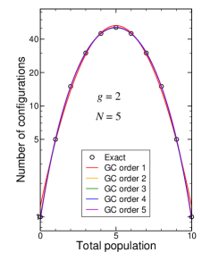
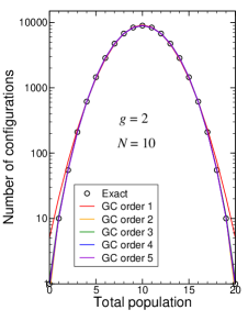
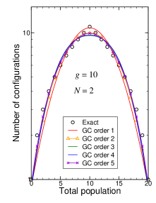
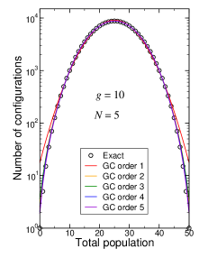
Using the above relations (84,88) we have compared the exact distribution $\mathscr{S}(g;N;Q)$ with Gram-Charlier expansions for several $(g,N)$ pairs on the whole $Q=0-g.N$ range of populations. Examples are given in Figs. 1 and 2 for $g=2$ and $g=10$ respectively. In each figure, cases $N=2,5$, and 10 have been studied. One observes that even the normal distribution, i.e., formula (84) with all $c_{k}$ canceled, provides a reasonable approximation of the $\mathscr{S}(g;N;Q)$ value. Looking in more detail, in the wings of the distribution, the inclusion of at least the 2nd-order correction $c_{4}He_{4}(X)$ in the Gram-Charlier expansion significantly improves the quality of the approximation. As mentioned above, the evaluation of such correction using the expression (88a) is straightforward.

(a) $N=2$

(b) $N=5$

(c) $N=10$

Figure 1: Comparison of the exact population distribution in $N$ subshells of degeneracy $g=2$ with Gram-Charlier expansions at various orders. The Gram-Charlier expansion is plotted as a continuous function of the total population $Q$. In this figure, “order $p$” means that moments up to $k=2p$ have been included in the expansion.

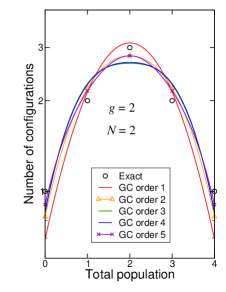
One may notice a visible, though moderate, discrepancy in the case $N=2$, whatever the $g$ value. This may be easily understood by computing directly the $\mathscr{S}(g;N=2;Q)$ value. Using the recursion relations (12) and the initial value (72) one may check that $\mathscr{S}(g;N;Q)$ expressed versus $Q$ are piecewise polynomials of degree $N-1$, with a unique definition on intervals of length $g$. Namely, one obtains

$$\mathscr{S}(g;2;Q)=g+1-\left|Q-g\right|$$ (89)

$$\mathscr{S}(g;3;Q)=\begin{cases}\frac{1}{2}(Q+1)(Q+2)&\text{ if }0\leq Q\leq g\\ \frac{1}{2}(g+1)(g+2)-(Q-g)(Q-2g)&\text{ if }g\leq Q\leq 2g\\ \frac{1}{2}(Q-3g-1)(Q-3g-2)&\text{ if }2g\leq Q\leq 3g\end{cases}.$$ (90)

Obviously, it quite difficult to approximate the triangle-shaped function (89) with a normal distribution. The approximations at the various orders Gram-Charlier of $\mathscr{S}(2;2;Q)$ are given in table 2. It turns out that the maximum discrepancy is about 10 %. For $Q=0$, the discrepancy decreases with the expansion order, while for $Q=1,2$ the first order is better than the next four orders. An optimum is reached at sixth order, and for higher orders the overall agreement deteriorates, with some oscillations. Finally, above 18th order, we have checked that the Gram-Charlier expansion clearly diverges. These considerations concern the convergence analysis of the Gram-Charlier expansion more than the computational interest of this series, since for the lowest $N$ values, as seen in the above mentioned examples, simple piecewise polynomial expressions are available.

$Q$	Exact	Order 1	Order 2	Order 3	Order 4	Order 5	Order 6	Order 7	Order 8
0	1	0.694	0.824	0.852	0.855	0.904	0.991	1.070	1.114
1	2	2.137	2.200	2.277	2.264	2.155	2.002	1.861	1.769
2	3	3.109	2.818	2.660	2.679	2.818	3.003	3.174	3.294

Table 2: Number of configurations as a function of the population $Q$ for $N=2$ subshells of degeneracy $g=2$: exact values and Gram-Charlier approximations. Order one is the normal distribution, order 2 includes the kurtosis contribution, etc.

(a) $N=2$

(b) $N=5$

(c) $N=10$

Figure 2: Comparison of the exact population distribution in $N$ subshells of degeneracy $g=10$ with Gram-Charlier expansions at various orders.

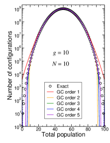
As seen in figure 2 dealing with a greater $g$ value, while the Gram-Charlier expansion at 2nd order (with the excess kurtosis accounted for) is quite acceptable in most of the $Q=0$ to $gN$ range, discrepancies are clearly visible for $Q\lesssim(gN)^{1/2}$, $Q\gtrsim gN-(gN)^{1/2}$. For such population values, the number of configurations $\mathscr{S}$ is usually orders of magnitude below its peak value $(g+1)^{N}/(2\pi\sigma^{2})^{1/2}$, however one may be interested in approximations uniformly valid whatever $Q$. In this case it appears that the inclusion of more terms in the Gram-Charlier expansion improves its accuracy in the wings. Though this behavior is clear on subfigure 2(c), we did not try to get a quantitative estimate of the Gram-Charlier order which provides a uniform approximation for the $\mathscr{S}(g=10;N=10;Q)$ values.

8.2 Multiple-degeneracy case

Using the general expression (108a) of the Gram-Charlier coefficients, and the cumulant value (80), one easily gets the first terms of the expansion

$$c_{4} =-\frac{C_{4}}{20C_{2}^{2}}$$ (91a)

$$c_{6} =\frac{C_{6}}{105C_{2}^{3}}$$ (91b)

$$c_{8} =\frac{7C_{4}^{2}-12C_{8}}{5600C_{2}^{4}}$$ (91c)

$$c_{10} =\frac{12C_{10}-11C_{4}C_{6}}{23100C_{2}^{5}}$$ (91d)

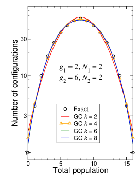
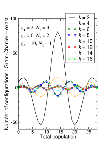
which generalize the Eqs. (88) in the multi-degeneracy case. Such a procedure has been used first to analyze the population distribution in the case $t=2,g_{1}=2,N_{1}=2,g_{2}=6,N_{2}=2$, labeled s[2]p[2] for short. The Gram-Charlier analysis is presented in figure 3(a). We note that, even though the number of subshells is small (4), the Gram-Charlier expansion with the first correction $c_{4}$ (orange curve and triangles) provides a fair approximation of the exact number. Moreover the Gram-Charlier formula, of statistical nature, would perform even better for more complex configurations with a greater number of subshells.

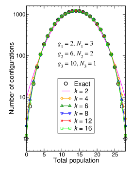
As a second example the Gram-Charlier approximation for the more complex supershell s[3]p[2]d[1] (for instance 1s2s2p3s3p3d) is analyzed on figure 3(b). One checks that Gram-Charlier at second order ($k=4$) is in fair agreement with the exact data. The 3rd order ($k=6$) improves again the agreement, with no significant gain at 4th order ($k=8$). The higher-order expansions $k=12,16$ bring an improved agreement with the exact value, especially for the smallest and largest $Q$ values.

(a) $g_{1}=2,N_{1}=2$, $g_{2}=6,N_{2}=2$

(b) $g_{1}=2,N_{1}=3$, $g_{2}=6,N_{2}=2$, $g_{3}=10,N_{3}=1$

Figure 3: Comparison of the exact population distribution with Gram-Charlier expansions at various orders for the supershell s[2]p[2] (two subshells s and two subshells p, for instance 2s2p3s3p) (a), and for the supershell s[3]p[2]d[1] (for instance 1s2s2p3s3p3d) (b).

As a rule one may check that the accuracy of the Gram-Charlier expansion globally increases with the order, though some oscillations are noticed. As an example, in figure 4 we have plotted the difference between the Gram-Charlier approximation (84) truncated at various orders and the exact number of configurations. In this particular case, a good compromise between the quality of the expansion and the computational cost is reached for $k=10$, i.e., with five terms in the sum. As shown below, a more complete numerical analysis involving higher orders demonstrates that the Gram-Charlier series is indeed divergent.

Figure 4: Difference between the number of configurations obtained with the Gram-Charlier expansion truncated at various orders and the exact value for the supershell 1s2s2p3s3p3d. The $k=2$ curve corresponds to the normal distribution, $k=4$ is the Gram-Charlier series involving up to the $He_{4}$ polynomial or second-order approximation, etc. Though exact values are only defined for integer populations $Q$, lines are drawn as a visual guide.

9 Analysis of population distribution using Edgeworth expansion

It has been mentioned that some distributions get a better representation in terms of Edgeworth series rather than of Gram-Charlier series [7]. Another interest of the Edgeworth expansion is that it is directly expressed in terms of cumulants rather than of centred moments. The Edgeworth series is an expansion versus powers of the standard deviation $\sigma$, defined as

$$E(Q)=G\frac{\exp(-x^{2}/2)}{\sqrt{2\pi}\sigma}\left\{1+\sum_{s=1}^{\infty}\sigma^{s}\sum_{\{k_{m}\}}He_{s+2r}(x)\prod_{m=1}^{s}\frac{1}{k_{m}!}\left(\frac{S_{m+2}}{(m+2)!}\right)^{k_{m}}\right\}$$ (92a)

$$\text{with\quad}S_{n}=\kappa_{n}/\sigma^{2n-2}\text{,\quad}r=k_{1}+k_{2}+\cdots k_{s}$$ (92b)

$$x$$ being the reduced variable

$$x=(Q-\left<Q\right>)/\sigma$$ (92c)

and where the index $$\{k_{m}\} s$$ refer to all -uple indices verifying

$$k_{1}+2k_{2}+\cdots+sk_{s}=s.$$ (92d)

As for Gram-Charlier expansion, this series involves only even $s$ orders. The sum over $s$ is replaced by a finite sum up to some $s_{\text{trunc}}$, which is chosen as discussed below.

Figure 5: Standard mean deviation $\left[\sum_{Q=0}^{Q_{\text{max}}}\left(N_{\text{app}}(Q;s_{\text{trunc}})-N_{\text{exact}}(Q)\right)^{2}/(Q_{\text{max}}+1)\right]^{1/2}$ for the number of configurations $Q$ computed exactly or using expansions truncated at various orders $s_{\text{trunc}}$. Configurations are generated from the $1s2s2p3s3p3d$ supershell and approximations are those obtained from Gram-Charlier and Edgeworth series. Only even $s_{\text{trunc}}$ values are plotted since odd-order terms in the expansions vanish.

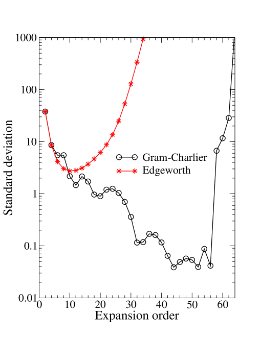
In order to compare Edgeworth and Gram-Charlier expansions we have plotted in figure 5 the average deviation

$$\Delta_{\text{app}}(s_{\text{trunc}})=\left[\sum_{Q=0}^{Q_{\text{max}}}\left(N_{\text{app}}(Q;s_{\text{trunc}})-N_{\text{exact}}(Q)\right)^{2}/(Q_{\text{max}}+1)\right]^{1/2}$$ (93)

for the $1s2s2p3s3p3d$ supershell as a function of $s_{\text{trunc}}$. In the above formula $Q_{\text{max}}$ is the maximum occupation number of the supershell $\sum_{i}g_{i}N_{i}$, 28 in the present case, $N_{\text{app}}(Q;s_{\text{trunc}})$ is the approximate number of configurations with occupation $Q$ computed with Gram-Charlier (84) or Edgeworth (92a) truncated series. A truncation order $s_{\text{trunc}}=2$ corresponds to the normal distribution, the truncation $s_{\text{trunc}}=4$ corresponds to terms involving the Chebyshev-Hermite polynomial $He_{4}(X)$, etc. On this graph, it appears that both expansions provide an acceptable representation of the number of configurations for the low values of $s_{\text{trunc}}$. Truncating the expansion at $s_{\text{trunc}}=10$, i.e., keeping four correction terms to the normal distribution, provides the best approximation in case of Edgeworth series. In this case, the relative error $\left[\sum_{Q=0}^{Q_{\text{max}}}\left(N_{\text{app}}(Q;s_{\text{trunc}})/N_{\text{exact}}(Q)-1\right)^{2}/(Q_{\text{max}}+1)\right]^{1/2}\simeq 0.4$ for Edgeworth expansion, while the absolute deviation plotted on figure 5 is 2.74. This apparently poor agreement is due to the large error in the $Q=0$ approximate value : $N_{\text{Edgeworth}}(Q=0;s_{\text{trunc}}=10)\simeq-0.519$ while $N_{\text{exact}}(Q=0)=1$. However large values around $Q_{\text{max}}/2$ are better represented : indeed one has $N_{\text{Edgeworth}}(Q=14;s_{\text{trunc}}=10)\simeq 1221.79,N_{\text{exact}}(Q=14)=1217$. The general behavior is quite different for $s_{\text{trunc}}$ above 10: while Gram-Charlier accuracy still improves with $s_{\text{trunc}}$, the Edgeworth-expansion accuracy deteriorates rapidly. As seen on the graph, for very large values ($s_{\text{trunc}}>56$), the Gram-Charlier expansion also diverges rapidly. This behavior has been mentioned previously [7], but our conclusion is that Gram-Charlier expansion provides here a better approximation than Edgeworth expansion. Our conclusion is also at variance with the observation by de Kock et al. [11] who claim that Edgeworth series strongly outperforms Gram-Charlier series. In our opinion this difference comes from the fact that we are dealing here with a discrete distribution, defined only for integer values, and that this distribution is not an analytical function of $Q$ but a piecewise polynomial.

10 Conclusion

We found three explicit formulas for the number of atomic configurations. Although the best way to compute such a quantity remains probably the double recurrence on the numbers of electrons and orbitals, the new expressions may be of interest in order to get new relations for the number of atomic configurations, using the numerous properties, identities and sum rules for binomial and multinomial coefficients. Using a two-variable generating function, we have derived several recurrence relations, not published before up to our knowledge. Using the same generating function, the moments of the distribution have received an analytical expression. It allowed us to provide explicit expressions for moments up to the twelfth, though higher-order moments could be obtained too. The case of multiple value for the subshell degeneracy has been addressed using the cumulant formalism. We have shown that the cumulants receive a very simple expression whatever the order. This allowed us to obtain centred moments explicitly for $k$ up to 12. A Gram-Charlier analysis has shown that an expansion with two terms is in acceptable if not fair agreement with the exact number of configurations, though the series is not convergent. We have found that the Edgeworth expansion provides an equivalent accuracy if few terms are kept, though it diverges much more rapidly than the Gram-Charlier series.

Appendix A Numbering the partitions defined by subset populations

The purpose of this appendix is to enumerate the partitions of $n$ distinct objects knowing that there are $n_{1}$ subsets of population 1, $n_{2}$ subsets of population 2, …$n_{k}$ subsets of population $k$. In the main text one has $n=k$ though this constraint is not required for the present derivation. Conversely one must have

$$n=n_{1}+2n_{2}+\cdots kn_{k}.$$ (94)

The generation of these partitions may be done in $k+1$ steps. In the first step, one selects the $n_{1}$ elements in single-element subsets, the $2n_{2}$ elements in twofold subsets, up to the $kn_{k}$ elements in the subsets of population $n_{k}$. The number of possibilities at this step is

$$p_{0}=\binom{n}{n_{1}}\binom{n-n_{1}}{2n_{2}}\dots\binom{n-n_{1}\cdots-(k-2)n_{k-2}}{(k-1)n_{k-1}}\binom{n-n_{1}\cdots-(k-1)n_{k-1}}{kn_{k}}=\frac{n!}{\prod_{j=1}^{k}(jn_{j})!}.$$ (95)

At the next $k$ steps one must choose, for any $j$ from 1 to $k$, how to partition $jn_{j}$ objects in $n_{j}$ subsets. This operation is performed by first selecting $j$ objects among $jn_{j}$, then $j$ more objects among $j(n_{j}-1)$, i.e., repeating the selection process $n_{j}-1$ times. When this multiple selection is completed, one gets $n_{j}!$ identical solutions, since the order of the subsets is not significant. Therefore the number of possibilities at step $j$ is

$$p_{j}=\frac{1}{n_{j}!}\binom{jn_{j}}{j}\binom{(j-1)n_{j}}{j}\cdots\binom{2j}{j}\binom{j}{j}=\frac{1}{n_{j}!}\frac{(jn_{j})!}{(j!)^{n_{j}}}.$$ (96)

Multiplying $p_{0}$ given by Eq. (95) by the product of $p_{j}$’s provided by Eq. (96) one gets the desired number of partitions

$$\mathscr{P}(n;n_{1},n_{2}\cdots,n_{k})=\frac{n!}{\prod_{j=1}^{k}n_{j}!(j!)^{n_{j}}}.$$ (97)

Appendix B Coefficients of the Gram-Charlier expansion as a function of the cumulants

The generating function of the cumulants is defined as

$$\mathscr{K}(t)=\sum_{n=1}^{\infty}\kappa_{n}\frac{t^{n}}{n!}=\log\left(\left<\exp(tQ)\right>\right).$$ (98)

In the case of the Gram-Charlier expansion the integral $\left<\exp(tQ)\right>$ is easily obtained as

$$e^{\mathscr{K}(t)}=\left<\exp(tQ)\right>=\int dQ\frac{\exp(tQ-Q^{2}/2\sigma^{2})}{\sqrt{2\pi\sigma^{2}}}\left[1+\sum_{n>2}c_{n}He_{n}(Q/\sigma)\right].$$ (99)

Using the Rodrigues formula for $He_{n}(X)$ and repeated integration by parts one easily gets

$$\int_{-\infty}^{+\infty}dQ\>e^{tQ-X^{2}/2\sigma^{2}}He_{n}(Q/\sigma)=(\sigma t)^{n}\exp(\sigma^{2}t^{2}/2)$$ (100)

from which one has the average over Gram-Charlier distribution

$$\left<\exp(tQ)\right>=\int_{-\infty}^{+\infty}dQ\;e^{tQ-X^{2}/2\sigma^{2}}\left[1+\sum_{n>2}c_{n}He_{n}(Q/\sigma)\right]=e^{\sigma^{2}t^{2}/2}\left[1+\sum_{n>2}(\sigma t)^{n}c_{n}\right].$$ (101)

The exponential of the generating function of cumulants is, for any centred distribution (i.e., such as $\kappa_{1}=0$),

$$e^{\mathscr{K}(t)}=\exp\left(\sum_{n=1}^{\infty}\kappa_{n}\frac{t^{n}}{n!}\right)=e^{\kappa_{2}t^{2}/2}\exp\left(\sum_{n=3}^{\infty}\kappa_{n}\frac{t^{n}}{n!}\right).$$ (102)

Identifying this expression with the average (101), one writes

$$1+\sum_{n\geq 3}(\sigma t)^{n}c_{n}=\exp\left(\sum_{n=3}^{\infty}\kappa_{n}\frac{t^{n}}{n!}\right)=\exp\left(\sum_{n=1}^{\infty}x_{n}\frac{t^{n}}{n!}\right)=\sum_{m=0}^{\infty}\frac{1}{m!}\left(\sum_{n=1}^{\infty}x_{n}\frac{t^{n}}{n!}\right)^{m}$$ (103a)

where we have defined

$$x_{1}=0\text{,\quad}x_{2}=0\text{,\quad}x_{n}=\kappa_{n}\text{ if }n\geq 3.$$ (103b)

The $m$th power in the sum (103a) may be computed with the identity (see section 24.1.2 in Ref. [1])

$$\left(\sum_{n=1}^{\infty}x_{n}\frac{t^{n}}{n!}\right)^{m}=m!\sum_{n=m}^{\infty}\frac{t^{n}}{n!}\sum_{a_{1},a_{2},\cdots a_{n}}\mathscr{P}(n;a_{1},a_{2}\cdots,a_{n})\>x_{1}^{a_{1}}x_{2}^{a_{2}}\cdots x_{n}^{a_{n}}$$ (104a)

with the above definition (97) of the partition number $$\mathscr{P} a_{1},a_{2},\cdots a_{n}$$, and where integer indices are constrained by

$$a_{1}+a_{2}+\cdots+a_{n}=m$$ (104b)

$$a_{1}+2a_{2}+\cdots+na_{n}=n.$$ (104c)

Identifying terms in $t^{n}$ in Eqs. (103a, 104a), one has

$$\sigma^{n}c_{n}=\frac{1}{n!}\sum_{m\leq n}\sum_{a_{1},a_{2},\cdots a_{n}}\mathscr{P}(n;a_{1},a_{2}\cdots,a_{n})\>x_{1}^{a_{1}}x_{2}^{a_{2}}\cdots x_{n}^{a_{n}}$$ (105)

where the sum on $a_{i}$ follows the constraints (104a). One will note that, since the $a_{i}$ are nonnegative, one has

$$m=a_{1}+a_{2}+\cdots+a_{n}\leq a_{1}+2a_{2}+\cdots+na_{n}=n,$$ (106)

therefore in the multiple sum (105) one may ignore the sum over $m$, since this index is only intended to collect terms in the sum. One has then

$$\sigma^{n}c_{n}=\frac{1}{n!}\sum_{a_{1},a_{2},\cdots a_{n}}\mathscr{P}(n;a_{1},a_{2}\cdots,a_{n})\>x_{1}^{a_{1}}x_{2}^{a_{2}}\cdots x_{n}^{a_{n}}$$ (107)

where only the second constraint (104c) has been kept. Accounting for $x_{i}$ definitions (103b), one notes that only terms with $a_{1}=0,a_{2}=0$ contribute and one gets the Gram-Charlier-series coefficient

$$c_{n} =\frac{1}{\sigma^{n}n!}\sum_{\begin{subarray}{c}a_{3},\cdots a_{n}\\ 3a_{3}+\cdots+na_{n}=n\end{subarray}}\mathscr{P}(n;0,0,a_{3}\cdots,a_{n})\>\kappa_{3}^{a_{3}}\cdots\kappa_{n}^{a_{n}}$$ (108a)

$$=\sum_{\begin{subarray}{c}a_{3},\cdots a_{n}\\ 3a_{3}+\cdots+na_{n}=n\end{subarray}}\frac{1}{a_{3}!}\left(\frac{\kappa_{3}}{3!\sigma^{3}}\right)^{a_{3}}\cdots\frac{1}{a_{n}!}\left(\frac{\kappa_{n}}{n!\sigma^{n}}\right)^{a_{n}}.$$ (108b)

References

- [1] M. Abramowitz and I.A. Stegun. Handbook of Mathematical Functions. National Bureau of Standards, Washington DC, USA, 1972.
- [2] G. Andrews. Theory of Partitions. Addison-Wesley, Reading, Mass., 1976.
- [3] A. B. Balantekin. Partition functions in statistical mechanics, symmetric functions, and group representations. Phys. Rev. E, 64:066105, Nov 2001.
- [4] A. Bar-Shalom, J. Oreg, W. H. Goldstein, D. Shvarts, and A. Zigler. Super-transition-arrays: A model for the spectral analysis of hot, dense plasma. Phys. Rev. A, 40(6):3183–3193, 1989.
- [5] J Bauche and C Bauche-Arnoult. Level and line statistic in atomic spectra. J. Phys. B: At. Mol. Opt. Phys., 20(8):1659–1677, 1987.
- [6] Jacques Bauche, Claire Bauche-Arnoult, and Olivier Peyrusse. Atomic properties in hot plasmas. Springer International Publishing, Cham, Switzerland, 2015.
- [7] S. Blinnikov and R. Moessner. Expansions for nearly gaussian distributions. Astron. Astrophys. Suppl. Ser., 130(1):193–205, 1998.
- [8] Debajit Chakraborty, James Dufty, and Valentin V. Karasiev. Chapter two - System-size dependence in grand canonical and canonical ensembles. In John R. Sabin and Remigio Cabrera-Trujillo, editors, Concepts of Mathematical Physics in Chemistry: A Tribute to Frank E. Harris - Part A, volume 71 of Advances in Quantum Chemistry, pages 11 – 27. Academic Press, 2015.
- [9] Louis Comtet. Advanced Combinatorics. D. Reidel Publishing Company, Dordrecht, The Netherlands, 1974.
- [10] M Crance. A statistical description for multiphoton stripping of atoms. J. Phys. B: At. Mol. Opt. Phys., 17(21):4333–4341, nov 1984.
- [11] M. B. de Kock, H. C. Eggers, and J. Schmiegel. Edgeworth versus Gram-Charlier series: x-cumulant and probability density tests. Physics of Particles and Nuclei Letters, 8(9):1023–1027, Dec 2011.
- [12] F. Gilleron and J.-C. Pain. Efficient methods for calculating the number of states, levels and lines in atomic configurations. High Energy Density Phys., 5(4):320 – 327, 2009.
- [13] Franck Gilleron and Jean-Christophe Pain. Stable method for the calculation of partition functions in the superconfiguration approach. Phys. Rev. E, 69:056117, May 2004.
- [14] R. Glück, D. Köppl, and G. Wirsching. Computational aspects of ordered integer partition with upper bounds. In V. Bonifaci, C. Demetrescu, and A. Marchetti-Spaccamela, editors, Experimental Algorithms, pages 9–90. Springer-Verlag, Berlin, Heidelberg, Germany, 2013.
- [15] J Katriel and A Novoselsky. Term multiplicities in the LS-coupling scheme. J. Phys. A: Math. Gen., 22(9):1245–1251, may 1989.
- [16] J. Katriel, R. Pauncz, and J. J. C. Mulder. Studies in the configuration interaction method. II. Generating functions and recurrence relations for the number of many-particle configurations. Int. J. Quantum Chem., 23(5):1855–1867, 1983.
- [17] D. S. Kosov, M. F. Gelin, and A. I. Vdovin. Calculations of canonical averages from the grand canonical ensemble. Phys. Rev. E, 77:021120, Feb 2008.
- [18] Xieyu Na and M. Poirier. High-order moments of spin-orbit energy in a multielectron configuration. Phys. Rev. E, 94:013206, Jul 2016.
- [19] J.-C. Pain. PhD thesis, Paris-Sud XI Orsay University, France, 2002.
- [20] J.-Ch. Pain, F. Gilleron, J. Bauche, and C. Bauche-Arnoult. Effect of third- and fourth-order moments on the modeling of unresolved transition arrays. High Energy Density Phys., 5(4):294 – 301, 2009.
- [21] J.-Ch. Pain, F. Gilleron, J. Bauche, and C. Bauche-Arnoult. Erratum to “effect of third- and fourth-order moments on the modeling of unresolved transition arrays” [High Energy Density Phys. 5(4)(2009) 294–301]. High Energy Density Phys., 6(3):356, 2010.
- [22] Jean-Christophe Pain, Franck Gilleron, Jacques Bauche, and Claire Bauche-Arnoult. Statistics of electric-quadrupole lines in atomic spectra. J. Phys. B: At. Mol. Opt. Phys., 45(13):135006, jun 2012.
- [23] Jean-Christophe Pain, Franck Gilleron, and Gérald Faussurier. Jensen-Feynman approach to the statistics of interacting electrons. Phys. Rev. E, 80:026703, Aug 2009.
- [24] Jean-Christophe Pain, Franck Gilleron, and Quentin Porcherot. Generating functions for canonical systems of fermions. Phys. Rev. E, 83:067701, Jun 2011.
- [25] S A Ponomarenko, M E Sherrill, D P Kilcrease, and G Csanak. Statistical mean-field theory of finite quantum systems: canonical ensemble formulation. J. Phys. A: Math. Gen., 39(30):L499–L505, jul 2006.
- [26] Scott Pratt. Canonical and microcanonical calculations for Fermi systems. Phys. Rev. Lett., 84:4255–4259, May 2000.
- [27] Alan Stuart and J. Keith Ord. Kendall’s Advanced Theory of Statistics – Distribution Theory, volume 1. John Wiley and Sons, London UK, 1994.
- [28] Brian G. Wilson, Franck Gilleron, and Jean-Christophe Pain. Further stable methods for the calculation of partition functions in the superconfiguration approach. Phys. Rev. E, 76:032103, Sep 2007.
- [29] G. Wirsching. Balls in constrained urns and Cantor-like sets. Zeit. Anal. Anwendungen, 17:979–996, 1998.
- [30] Renjun Xu and Zhenwen Dai. Alternative mathematical technique to determine LS spectral terms. J. Phys. B: At. Mol. Opt. Phys., 39(16):3221–3239, jul 2006.