Glancing Transformer for Non-Autoregressive
Neural Machine Translation

Abstract

Recent work on non-autoregressive neural machine translation (NAT) aims at improving the efficiency by parallel decoding without sacrificing the quality. However, existing NAT methods are either inferior to Transformer or require multiple decoding passes, leading to reduced speedup. We propose the Glancing Language Model (GLM), a method to learn word interdependency for single-pass parallel generation models. With GLM, we develop Glancing Transformer (GLAT) for machine translation. With only single-pass parallel decoding, GLAT is able to generate high-quality translation with 8$\times$-15$\times$ speedup. Experiments on multiple WMT language directions show that GLAT outperforms all previous single pass non-autoregressive methods, and is nearly comparable to Transformer, reducing the gap to 0.25-0.9 BLEU points.

1 Introduction

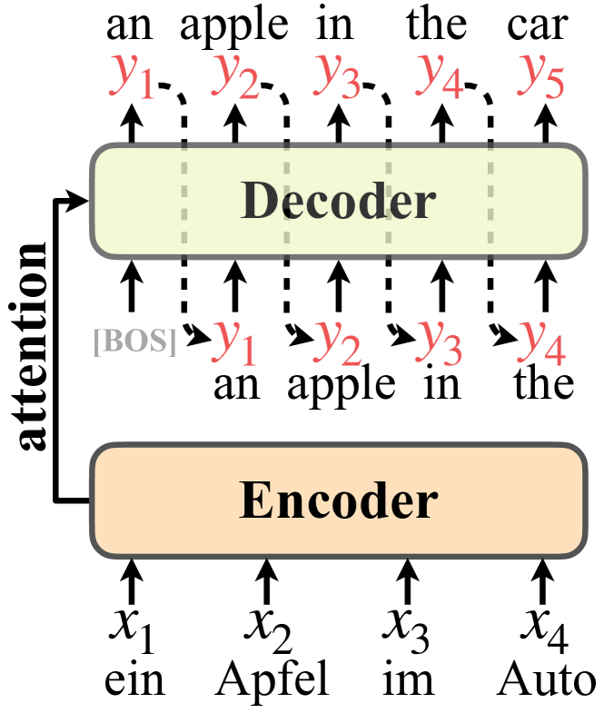
(a) Sequential LM

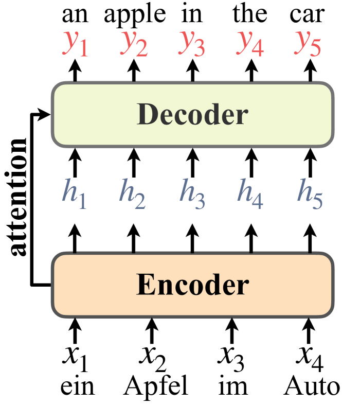
(b) Cond. Independent LM

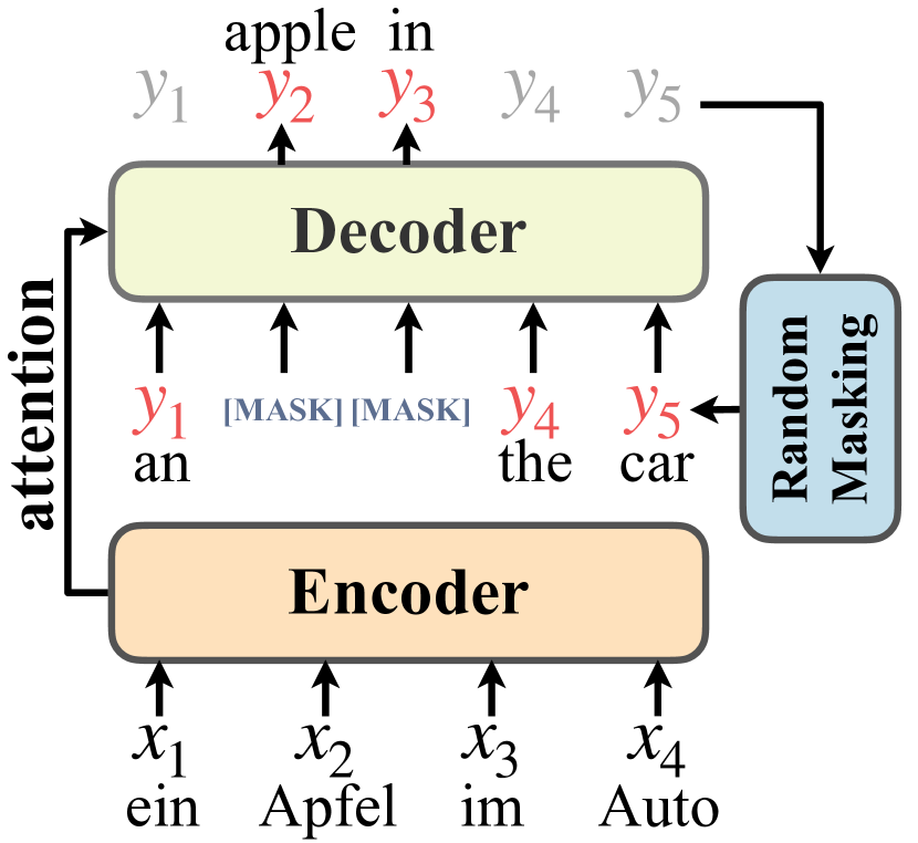
(c) Masked LM (MLM)

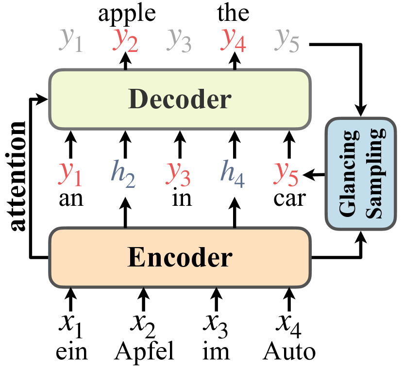
(d) Glancing LM (GLM)

Figure 1: Probabilistic models for machine translation methods. (1(b)) Vanilla NAT uses conditional indepedent LM. (1(c)) Mask-Predict NAT uses MLM and requires multiple passes of decoding. (1(d)) Our proposed GLM leverages the decoder prediction to decide glancing sampling policy during training and only requires one pass of decoding during inference.

Transformer has been the most widely used architecture for machine translation (Vaswani et al., 2017). Despite its strong performance, the decoding of Transformer is inefficient as it adopts the sequential auto-regressive factorization for its probability model (Figure 1(a)). Recent work such as non-autoregressive transformer (NAT), aim to decode target tokens in parallel to speed up the generation (Gu et al., 2018). However, the vanilla NAT still lags behind Transformer in the translation quality – with a gap about 7.0 BLEU score. NAT assumes the conditional independence of the target tokens given the source sentence. We suspect that NAT’s conditional independence assumption prevents learning word interdependency in the target sentence. Notice that such word interdependency is crucial, as the Transformer explicitly captures that via decoding from left to right (Figure 1(a)).

Several remedies are proposed (Ghazvininejad et al., 2019; Gu et al., 2019) to capture word interdependency while keeping parallel decoding. Their common idea is to decode the target tokens iteratively while each pass of decoding is trained using the masked language model (Figure 1(c)). Since these methods require multiple passes of decoding, its generation speed is measurably slower than the vanilla NAT. With single-pass generation only, these methods still largely lag behind the autoregressive Transformer.

One open question is whether a complete parallel decoding model can achieve comparable machine translation performance to the Transformer. It should be non-autoregressive and take only one pass of decoding during the inference time.

To address the quest, we propose glancing language model (GLM), a new method to train a probabilistic sequence model. Based on GLM, we develop the glancing Transformer (GLAT) for neural machine translation. It achieves parallel text generation with only single decoding pass. Yet, it outperforms previous NAT methods and achieves comparable performance as the strong Transformer baseline in multiple cases. Intuitively, GLM adopts a adaptive glancing sampling strategy, which glances at some fragments of the reference if the reference is too difficult to fit in the training of GLAT. Correspondingly, when the model is well tuned, it will adaptively reduce the percentage of glancing sampling, making sure that the resulting model could learn to generate the whole sentence in the single-pass fashion.

Specifically, our proposed GLM differs from MLM in two aspects. Firstly, GLM proposes an adaptive glancing sampling strategy, which enables GLAT to generate sentences in a one-iteration way, working by gradual training instead of iterative inference (see Figure 1(d)). Generally, GLM is quite similar to curriculum learning (Bengio et al., 2009) in spirit, namely first learning to generate some fragments and gradually moving to learn the whole sentences (from easy to hard). To achieve the adaptive glancing sampling, GLM performs decoding twice in training. The first decoding is the same as the vanilla NAT, and the prediction accuracy indicates whether the current reference is “difficult” for fitting. In the second decoding, GLM gets words of the reference via glancing sampling according to the first decoding, and learn to predict the remaining words that are not sampled. Note that only the second decoding will update the model parameters. Secondly, instead of using the [MASK] token, GLM directly uses representations from the encoder at corresponding positions, which is more natural and could enhance the interactions between sampled words and signals from the encoder.

Experimental results show that GLAT obtains significant improvements (about 5 BLEU) on standard benchmarks compared to the vanilla NAT, without losing inference speed-up. GLAT achieves competitive results against iterative approaches like Mask-Predict (Ghazvininejad et al., 2019), even outperforming the Mask-Predict model on WMT14 DE-EN and WMT16 RO-EN. Compared to the strong AT baseline, GLAT can still close the performance gap within 0.9 BLEU point while keeping $7.9\times$ speed-up. Empirically, we even find that GLAT outperforms AT when the length of the reference is less than 20 on WMT14 DE-EN. We speculate this is because GLM could capture bidirectional context for generation while its left-to-right counterpart is only unidirectional, which indicates the potential of parallel generation approaches like GLAT.

2 Probability Models of Machine Translation

We state and compare different probability models for machine translation. A machine translation task can be formally defined as a sequence to sequence generation problem: given the source sentence $X=\{x_{1},x_{2},...,x_{N}\}$, to generate the target sentence $Y=\{y_{1},y_{2},...,y_{T}\}$ according to the conditional probability $P(Y|X;\theta)$, where $\theta$ denotes the parameter set of a network. Different methods factorize the conditional probability differently.

The Transformer uses the autoregressive factorization to maximize the following likelihood:

$$\mathcal{L}_{\text{AT}}=\log P(Y|X;\theta)=\sum_{t=1}^{T}\log p(y_{t}|y_{<t},X;\theta),$$

where $y_{<t}=\{\texttt{[BOS]},y_{1},...,y_{t-1}\}$. For simplicity, we omit the number of samples in the equation. Note the training of AT adopts left-to-right teacher forcing on the target tokens (Vaswani et al., 2017). The word interdependency is learned in a unidirectional way. During inference, the preceding predicted token is fed into the decoder to generate the next token.

The vanilla NAT consists of the same encoder as Transformer and a parallel decoder with layers of multi-head attention (Gu et al., 2018). During training, it uses the conditional independent factorization for the target sentence:

$$\mathcal{L}_{\text{NAT}}=\sum_{t=1}^{T}\log P(y_{t}|X;\theta).\\$$

Notice that, NAT’s log-likelihood is an approximation to the full log-likelihood $\log P(Y|X;\theta)$. During inference, the encoder representation is copied as the input to the decoder, therefore all tokens on the target side can be generated in parallel. Such a conditional independence assumption does not hold in general, which explains the inferior performance of NAT.

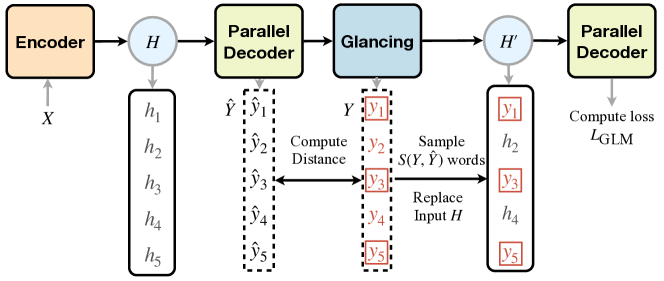
Figure 2: The training procedure with glancing sampling in GLAT. $H$ is the representation computed by the encoder. $\hat{y}$’s are the initial predicted tokens of the parallel decoder. $y$’s are the ground-truth target tokens. $H^{\prime}$ is fed into the decoder again to calculate the training loss.

Multi-pass iterative decoding approaches such as Mask-Predict (Ghazvininejad et al., 2019) extends the vanilla NAT. It still uses the conditional independent factorization, together with the random masking scheme:

$$\mathcal{L}_{\text{MLM}}=\sum_{y_{t}\in\mathbb{RM}(Y)}\log p\Big{(}y_{t}|\Phi\big{(}Y,\mathbb{RM}(Y)\big{)},X;\theta\Big{)},$$

where $\mathbb{RM}(Y)$ is a set of randomly selected words from $Y$, and $\Phi(\cdot)$ replaces these selected words in $Y$ with the [MASK] token. For example in Figure 1(c), $\mathbb{RM}(Y)=\{y_{2},y_{3}\}$, $\Phi\big{(}Y,\mathbb{RM}(Y)\big{)}=\{y_{1},\texttt{[MASK]},\texttt{[MASK]},y_{4},y_{5}\}$. The training objective is to learn a refinement model $\theta$ that can predict the masked tokens given the source sentence $X$ and words generated in the previous iteration.

The vanilla NAT breaks word interdependency, while MLM requires multiple passes of decoding to re-establish the word interdependency. Our goal in this work is to design a better probability model and a training objective to enable word interdependency learning for single-pass parallel generation.

3 Glancing Transformer

In this section, we present GLAT in detail. GLAT uses the same encoder-decoder architecture as the vanilla NAT (Gu et al., 2018). GLAT differs from the vanilla NAT in that it explicitly encourages word interdependency via training with glancing language model (GLM). It differs from the iterative NAT with MLM in that it is trained to produce single pass parallel decoding while MLM is used for prediction refinement.

3.1 The Glancing Language Model

Given the input source sentence $X=\{x_{1},x_{2},...,x_{N}\}$, the task is to predict $Y=\{y_{1},y_{2},...,y_{T}\}$. The glancing Transformer (GLAT) formulates a glancing language model (GLM) during training. It maximizes the following:

$$\mathcal{L}_{\text{GLM}}=\sum_{y_{t}\in\overline{\mathbb{GS}(Y,\hat{Y})}}\\ \log p(y_{t}|\mathbb{GS}(Y,\hat{Y}),X;\theta)$$ (1)

Where, $\hat{Y}$ is an initial predicted tokens, and $\mathbb{GS}(Y,\hat{Y})$ is a subset of tokens selected via the glancing sampling strategy (Figure 2, described in detail in the next section). The glancing sampling strategy selects those words from the target sentence by comparing the initial prediction against the ground-truth tokens. It selects more tokens and feeds them into the decoder input if the network’s initial prediction is less accurate. $\overline{\mathbb{GS}(Y,\hat{Y})}$ is the remaining subset of tokens within the target $Y$ but not selected. The training loss above is calculated against these remaining tokens.

GLAT adopts similar encoder-decoder architecture as the Transformer with some modification (Figure 1(d)). Its encoder $f_{\text{enc}}$is the same multi-head attention layers. Its decoder $f_{\text{dec}}$ include multiple layers of multi-head attention where each layer attends to the full sequence of both encoder representation and the previous layer of decoder representation.

During the initial prediction, the input to the decoder $H=\{h_{1},h_{2},...,h_{T}\}$ are copied from the encoder output using either uniform copy or soft copy (Wei et al., 2019). The initial tokens $\hat{Y}$ are predicted using $\operatorname{argmax}$ decoding with $f_{\text{dec}}(f_{\text{enc}}(X;\theta),H;\theta)$.

To calculate the loss $\mathcal{L}_{\text{GLM}}$, we compare the initial prediction $\hat{Y}$ against the ground-truth to select tokens within the target sentence, i.e. $\mathbb{GS}(Y,\hat{Y})$. We then replace those sampled indices of $h$’s with corresponding target word embeddings, $H^{\prime}=\mathbb{RP}(\text{Emb}_{y_{t}\in\mathbb{GS}(Y,\hat{Y})}(y_{t}),H)$, where $\mathbb{RP}$ replaces the corresponding indices. Namely, if a token in the target is sampled, its word embedding replaces the corresponding $h$. Here the word embeddings are obtained from the softmax embedding matrix of the decoder. The updated $H^{\prime}$ is then fed into the decoder $f_{\text{dec}}$ again to calculate the output token probability. Specifically, the output probabilities of remaining tokens $p(y_{t}|\mathbb{GS}(Y,\hat{Y}),X;\theta)$ are computed with $f_{\text{dec}}(H^{\prime},f_{\text{enc}}(X;\theta);\theta)$.

3.2 The Glancing Sampling Strategy

One important component of GLM is to adaptively select the positions of tokens from the target sentence. Those selected tokens provide “correct” information from the ground-truth target, therefore it helps training the decoder to predict the rest non-selected tokens. Intuitively, our adaptive sampling strategy guides the model to first learn the generation of fragments and then gradually turn to the whole sentences. Our glancing sampling strategy selects many words at the start of the training, when the model is not yet well tuned. As the model gets better progressively, the sampling strategy will sample fewer words to enable the model to learn the parallel generation of the whole sentence. Note that the sampling strategy is crucial in the training of GLAT.

As illustrated in Figure 2, the glancing sampling could be divided into two steps: first deciding a sampling number $S$, and then randomly selecting $S$ words from the reference. The sampling number $S$ will be larger when the model is poorly trained and decreases along the training process. Note that we choose to randomly select the $S$ words from the reference. The random reference word selection is simple and yields good performance empirically.

Formally, given the input $X$, its predicted sentence $\hat{Y}$ and its reference $Y$, the goal of glancing sampling function $\mathbb{GS}(Y,\hat{Y})$ is to obtain a subset of words sampled from $Y$:

$$\mathbb{GS}(Y,\hat{Y})=\text{Random}(Y,S(Y,\hat{Y}))$$ (2)

Here, $\text{Random}(Y,S)$ is randomly selecting $S$ tokens from $Y$, and $S$ is computed by comparing the difference between $\hat{Y}$ and $Y$, $S(Y,\hat{Y})=\lambda\cdot d(Y,\hat{Y})$. The sampling ratio $\lambda$ is a hyper-parameter to more flexibly control the number of sampled tokens. $d(Y,\hat{Y})$ is a metric for measuring the differences between $Y$ and $\hat{Y}$. We adopt the Hamming distance (Hamming, 1950) as the metric, which is computed as $d(Y,\hat{Y})=\sum_{t=1}^{T}(y_{t}\neq\hat{y}_{t})$. With $d(Y,\hat{Y})$, the sampling number can be decided adaptively considering the current trained model’s prediction capability. For situations that $Y$ and $\hat{Y}$ have different lengths, $d(Y,\hat{Y})$ could be other distances such as Levenshtein distance (Levenshtein, 1966).

Alternative glancing sampling strategy can be adopted as well. For example, one simple alternative strategy is to set the number of sampled tokens to be proportional to the target sentence length, i.e. $S=\lambda*T$. We will evaluate the effects of these variations in the experiment.

3.3 Inference

GLAT only modifies the training procedure. Its inference is fully parallel with only a single pass. For parallel generation, we need to decide the output lengths before decoding. A simple way to decide the output lengths is predicting length with representations from the encoder.

In GLAT, the length prediction is implemented as in Ghazvininejad et al. (2019). An additional [LENGTH] token is added to the source input, and the encoder output for the [LENGTH] token is used to predict the length.

We also use two more complex methods to better decide the output lengths: noisy parallel decoding (NPD) and connectionist temporal classification (CTC). For NPD (Gu et al., 2018), we first predict $m$ target length candidates, then generate output sequences with $\operatorname{argmax}$ decoding for each target length candidate. Then we use a pre-trained transformer to rank these sequences and identify the best overall output as the final output. For CTC (Graves et al., 2006), following Libovickỳ and Helcl (2018), we first set the max output length to twice the source input length, and remove the blanks and repeated tokens after generation.

4 Experiments

Models			$I_{\text{dec}}$	WMT14		WMT16		Speed Up
				EN-DE	DE-EN	EN-RO	RO-EN
AT Models		Transformer (Vaswani et al., 2017)	T	27.30	/	/	/	/
		Transformer (ours)	T	27.48	31.27	33.70	34.05	1.0$\times$
Iterative NAT		NAT-IR (Lee et al., 2018)	10	21.61	25.48	29.32	30.19	1.5$\times$
		LaNMT (Shu et al., 2020)	4	26.30	/	/	29.10	5.7$\times$
		LevT (Gu et al., 2019)	6+	27.27	/	/	33.26	4.0$\times$
		Mask-Predict (Ghazvininejad et al., 2019)	10	27.03	30.53	33.08	33.31	1.7$\times$
		JM-NAT (Guo et al., 2020)	10	27.31	31.02	/	/	5.7$\times$
Fully NAT		NAT-FT (Gu et al., 2018)	1	17.69	21.47	27.29	29.06	15.6$\times$
		Mask-Predict (Ghazvininejad et al., 2019)	1	18.05	21.83	27.32	28.20	/
		imit-NAT (Wei et al., 2019)	1	22.44	25.67	28.61	28.90	18.6$\times$
		NAT-HINT (Li et al., 2019)	1	21.11	25.24	/	/	/
		Flowseq (Ma et al., 2019)	1	23.72	28.39	29.73	30.72	1.1$\times$
		NAT-DCRF (Sun et al., 2019)	1	23.44	27.22	/	/	10.4 $\times$
	w/ CTC	NAT-CTC (Libovickỳ and Helcl, 2018)	1	16.56	18.64	19.54	24.67	/
		Imputer (Saharia et al., 2020)	1	25.80	28.40	32.30	31.70	18.6$\times$
	w/ NPD	NAT-FT + NPD (m=100)	1	19.17	23.20	29.79	31.44	2.4$\times$
		imit-NAT + NPD (m=7)	1	24.15	27.28	31.45	31.81	9.7$\times$
		NAT-HINT + NPD (m=9)	1	25.20	29.52	/	/	/
		Flowseq + NPD (m=30)	1	25.31	30.68	32.20	32.84	/
		NAT-DCRF + NPD (m=9)	1	26.07	29.68	/	/	6.1$\times$
	Ours	NAT-base*	1	20.36	24.81	28.47	29.43	15.3$\times$
		CTC*	1	25.52	28.73	32.60	33.46	14.6 $\times$
		GLAT	1	25.21	29.84	31.19	32.04	15.3$\times$
		GLAT + CTC	1	26.39	29.54	32.79	33.84	14.6 $\times$
		GLAT + NPD  (m=7)	1	26.55	31.02	32.87	33.51	7.9$\times$

Table 1: Results on WMT14 EN-DE/DE-EN and WMT16 EN-RO/RO-EN benchmarks. $I_{\text{dec}}$ is the number of decoding iterations and $m$ is the number of length reranking candidates. NPD represents noisy parallel decoding, CTC represents connectionist temporal classification. * indicate the results are obtained by our implementation.

In this section, we first introduce the settings of our experiments, then report the main results compared with several strong baselines. Ablation studies and further analysis are also included to verify the effects of different components used in GLAT.

4.1 Experimental Settings

Datasets

We conduct experiments on three machine translation benchmarks: WMT14 EN-DE (4.5M translation pairs), WMT16 EN-RO (610k translation pairs), and IWSLT16 DE-EN (150K translation pairs). These datasets are tokenized and segmented into subword units using BPE encodings (Sennrich et al., 2016). We preprocess WMT14 EN-DE by following the data preprocessing in Vaswani et al. (2017). For WMT16 EN-RO and IWSLT16 DE-EN, we use the processed data provided in Lee et al. (2018).

Knowledge Distillation

Following previous work (Gu et al., 2018; Lee et al., 2018; Wang et al., 2019), we also use sequence-level knowledge distillation for all datasets. We employ the transformer with the base setting in  Vaswani et al. (2017) as the teacher for knowledge distillation. Then, we train our GLAT on distilled data.

Baselines and Setup

We compare our method with the base Transformer and strong representative NAT baselines in Table 1. For all our tasks, we obtain other NAT models’ performance by directly using the performance figures reported in their papers if they are available.

We adopt the vanilla model which copies source input uniformly in Gu et al. (2018) as our base model (NAT-base) and replace the UniformCopy with attention mechanism using positions. Note that the output length does not equal the length of reference in models using CTC. Therefore, for GLAT with CTC, we adopt longest common subsequence distance for comparing $Y$ and $\hat{Y}$, and the glancing target is the target alignment that maximize the output probability $arg\max_{a\in\mathcal{B}^{-1}(Y)}P(a|X;\theta)$. $\mathcal{B}^{-1}$ is the mapping proposed in (Graves et al., 2006), which expand the reference to the length of output by inserting blanks or repeating words.

For WMT datasets, we follow the hyperparameters of the base Transformer in Vaswani et al. (2017). And we choose a smaller setting for IWSLT16, as IWSLT16 is a smaller dataset. For IWSLT16, we use 5 layers for encoder and decoder, and set the model size $d_{\text{model}}$ to 256. Using Nvidia V100 GPUs, We train the model with batches of 64k/8k tokens for WMT/IWSLT datasets, respectively. We set the dropout rate to 0.1 and use Adam optimizer (Kingma and Ba, 2014) with $\beta=(0.9,0.999)$. For WMT datasets, the learning rate warms up to $5e-4$ in 4k steps and gradually decays according to inverse square root schedule in Vaswani et al. (2017). As for IWSLT16 DE-EN, we adopt linear annealing (from $3e-4$ to $1e-5$) as in Lee et al. (2018). For the hyper-parameter $\lambda$, we adopt linear annealing from 0.5 to 0.3 for WMT datasets and a fixed value of 0.5 for IWSLT16. The final model is created by averaging the 5 best checkpoints chosen by validation BLEU scores.

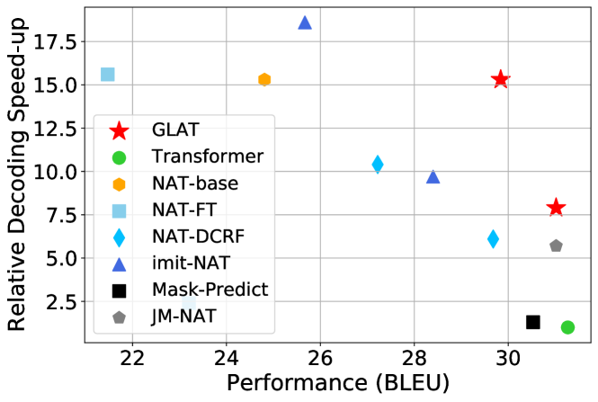
Figure 3: The trade-off between speed-up and BLEU on WMT14 DE-EN

4.2 Main Results

The main results on the benchmarks are presented in Table 1. GLAT significantly improves the translation quality and outperforms strong baselines by a large margin. Our method introduces explicit word interdependency modeling for the decoder and gradually learns simultaneous generation of whole sequences, enabling the model to better capture the underlying data structure. Compared to models with iterative decoding, our method completely maintains the inference efficiency advantage of fully non-autoregressive models, since GLAT generate with a single pass. Compared with the baselines, we highlight our empirical advantages:

• GLAT is highly effective. Compared with the vanilla NAT-base models, GLAT obtains significant improvements (about 5 BLEU) on EN-DE/DE-EN. Additionally, GLAT also outperforms other fully non-autoregressive models with a substantial margin (almost +2 BLEU score on average). The results are even very close to those of the AT model, which shows great potential.

• GLAT is simple and can be applied to other NAT models flexibly, as we only modify the training process by reference glancing while keeping inference unchanged. For comparison, NAT-DCRF utilizes CRF to generate sequentially; NAT-IR and Mask-Predict models need multiple decoding iterations.

• CTC and NPD use different approaches to determine the best output length, and they have their own advantages and disadvantages. CTC requires the output length to be longer than the exact target length. With longer output lengths, the training will consume more time and GPU memory. As for NPD, with a certain number of length reranking candidates, the inference speed will be slower than models using CTC. Note that NPD can use pretrained AT models or the non-autoregressive model itself to rerank multiple outputs.

We also present a scatter plot in Figure 3, displaying the trend of speed-up and BLEU with different NAT models. It is shown that the point of GLAT is located on the top-right of the competing methods. Obviously, GLAT outperforms our competitors in BLEU if speed-up is controlled, and in speed-up if BLEU is controlled. This indicates that GLAT outperforms previous state-of-the-art NAT methods. Although iterative models like Mask-Predict achieves competitive BLEU scores, they only maintain minor speed advantages over AT. In contrast, fully non-autoregressive models remarkably improve the inference speed.

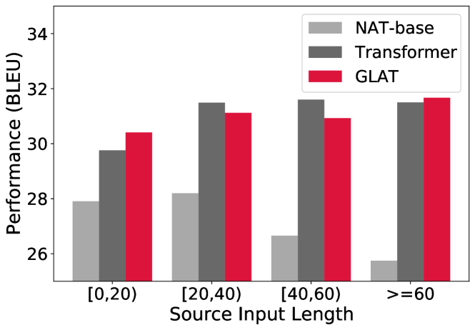
Figure 4: Performance under different source input length on WMT14 DE-EN

4.3 Analysis

Effect of Source Input Length

To analyze the effect of source input length on the models’ performance, we split the source sentences into different intervals by length after BPE and compute the BLEU score for each interval. The histogram of results is presented in Figure 4. NAT-base’s performance drops sharply for long sentences, while the gradual learning process enables GLAT to boost the performance by a large margin, especially for long sentences. We also find that GLAT outperforms autoregressive Transformer when the source input length is smaller than 20.

GLAT Reduces Repetition

We also measure the percentage of repeated tokens on test set of WMT14 EN-DE and WMT14 DE-EN. Table 2 presents the token repetition ratio of sentences generated by NAT-base and GLAT. The results show that GLAT significantly reduces the occurrence of repetition, and the repetition ratio can be further reduced with NPD. We think an important cause of the improvement is better interdependency modeling. Since GLAT explicitly encourages word interdependency modeling to better capture the dependency between target tokens, wrong generation patterns, such as repetition, can be largely avoided.

Model	WMT14
	EN-DE	DE-EN
NAT-base	8.32%	7.10%
GLAT	1.19%	1.05%
GLAT w/ NPD	0.32%	0.16%

Table 2: Token repetition ratio on WMT14 EN-DE and WMT14 DE-EN

4.4 Ablation Study

Effectiveness of the Adaptive Sampling Number

To validate the effectiveness of the adaptive sampling strategy for the sampling number $S(Y,\hat{Y})$, we also introduce two fixed approaches for comparison. The first one decides the sampling number with $\lambda*T$, where $T$ is the length of $Y$, and $\lambda$ is a constant ratio. The second one is relatively flexible, which sets a start ratio of $\lambda_{s}$ and an end ratio $\lambda_{e}$, and linearly reduces the sampling number from $\lambda_{s}*T$ to $\lambda_{e}*T$ along the training process.

As shown in Table 3 and Table 4, clearly, our adaptive approach (Adaptive in the table) outperforms the baseline models with big margins. The results confirm our intuition that the sampling schedule affects the generation performance of our NAT model. The sampling strategy, which first offers relatively easy generation problems and then turns harder, benefits the final performance. Besides, even with the simplest constant ratio, GLAT still achieves remarkable results. When set $\lambda=0.2$, it even outperforms the baseline $\lambda=0.0$ by 2.5 BLEU score.

The experiments potentially support that it is beneficial to learn the generation of fragments at the start and gradually transfer to the whole sequence. The flexible decreasing ratio method works better than the constant one, and our proposed adaptive approaches achieve the best results.

Sampling Number	$\lambda$	BLEU
Fixed	0.0	24.66
	0.1	24.91
	0.2	27.12
	0.3	24.98
	0.4	22.96
Adaptive	-	29.61

Table 3: Performances on IWSLT16 with fixed sampling ratio.

Sampling Number	$\lambda_{s}$	$\lambda_{e}$	BLEU
Decreasing	0.5	0	27.80
	0.5	0.1	28.21
	0.5	0.2	27.15
	0.5	0.3	23.37
Adaptive	-		29.61

Table 4: Performances on IWSLT16 with decreasing sampling ratio.

Influence of Reference Word Selection

To analyze how the strategies of selecting reference words affect glancing sampling, we conduct experiments with different selection strategies. By default, we assume all the words in the reference are equally important and randomly choose reference words for glancing. Besides the random strategy, we devise four other selection methods considering the prediction of first decoding. For $p_{\text{ref}}$ and $1-p_{\text{ref}}$, the sampling probability of each reference word is proportional to the output probability for the reference word $p_{\text{ref}}$ and the probability $1-p_{\text{ref}}$, respectively. Similar to the word selection strategy for masking words during inference in Mask-Predict, we also add two strategies related to the prediction confidence: "most certain" and "most uncertain." We choose the positions where predictions have higher confidence for "most certain", and vise versa for "most uncertain." The results for different selection methods are listed in Table 5.

In comparisons, the model with the selection strategy $1-p_{\text{ref}}$ outperforms the one with $p_{\text{ref}}$, indicating that words hard to predict are more important for glancing in training. And we find that the random strategy performs a little better than the two confidence-based strategies. We think this indicates that introducing more randomness in sampling enable GLAT to explore more interdependency among target words. We adopt the random strategy for its simplicity and good performance.

Selection Strategy	GLAT	GLAT w/ NPD
random	25.21	26.55
$p_{\text{ref}}$	24.87	25.83
$1-p_{\text{ref}}$	25.37	26.52
most certain	24.99	26.22
most uncertain	24.86	26.13

Table 5: Performance on WMT14 EN-DE with different reference word selection strategies.

Method	WMT14
	EN-DE	DE-EN
GLAT w/ uniform sampling	19.16	23.56
GLAT w/ [MASK] inputs	24.99	29.48
GLAT	25.21	29.84

Table 6: Ablation study for comparing GLAT and Mask-Predict on WMT14 EN-DE and DE-EN.

Advantages of GLAT over Mask-Predict

To study the effects of sampling strategy and decoder inputs of GLAT, we conduct experiments for replacing these two modules in GLAT with the corresponding part in Mask-Predict, respectively. The results are presented in Table 6. GLAT employs glancing sampling strategy instead of the uniform sampling strategy used in Mask-Predict, and replaces the [MASK] token inputs with source representations from the encoder. The results show that the glancing sampling strategy outperforms the uniform sampling strategy by 5$\sim$6 BLEU points, and feeding representations from the encoder as the decoder input could still improve the strong baseline by 0.2$\sim$0.3 BLEU points after adopting glancing sampling. To sum up, the adaptive glancing sampling approach contributes the most to the final improvement, and the use of representations from the encoder also helps a bit.

More Analysis

We also conduct experiments for: a) comparison of different distance metrics for glancing sampling, b) GLAT with more than one decoding iteration. The details are in Appendix.

5 Related Work

Fully Non-Autoregressive Models

A line of work introduces various forms of latent variables to reduce the model’s burden of dealing with dependencies among output words  (Gu et al., 2018; Ma et al., 2019; Bao et al., 2019; Ran et al., 2019). Another branch of work considers transferring the knowledge from autoregressive models to non-autoregressive models (Wei et al., 2019; Li et al., 2019; Guo et al., 2019b; Sun and Yang, 2020). Besides, there are also some work that apply different training objectives to train non-autoregressive models (Libovickỳ and Helcl, 2018; Shao et al., 2020; Ghazvininejad et al., 2020a), add regularization terms (Wang et al., 2019; Guo et al., 2019a).

Non-Autoregressive Models with Structured Decoding

To model the dependencies between words, Sun et al. (2019) introduces a CRF inference module in NAT and performs additional sequential decoding after the non-autoregressive computation in inference. Deng and Rush (2020) proposes cascaded CRF decoding. Since GLAT only performs single-pass non-autoregressive generation, our approach is orthogonal to the method proposed in Sun et al. (2019). We can also combine our approach with the structured decoding methods.

Non-Autoregressive Models with Iterative Refinement

A series of work are devoted to semi-autoregressive models that refine the outputs with multi-pass iterative decoding (Lee et al., 2018; Gu et al., 2019; Ghazvininejad et al., 2019, 2020b; Kasai et al., 2020).  Lee et al. (2018) proposed a method of iterative refinement based on denoising autoencoder.  Gu et al. (2019) utilized insertion and deletion to refine the outputs in inference.  Ghazvininejad et al. (2019) trained the model with the masked language model, and the model iteratively replaces masked tokens with new outputs. Despite the relatively better accuracy, the multiple decoding iterations vastly reduce the inference efficiency of non-autoregressive models.

6 Conclusion

In this paper, we propose Glancing Transformer with a glancing language model to improve the performance of single-pass parallel generation models. With the glancing language model, the model starts from learning the generation of sequence fragments and gradually moving to whole sequences. Experimental results show that our approach significantly improves the performance of non-autoregressive machine translation with single-pass parallel generation. As GLAT achieves competitive performance compared with autoregressive models, applying our approach to other generation tasks is a promising direction for future work.

References

- Bao et al. (2019) Yu Bao, Hao Zhou, Jiangtao Feng, Mingxuan Wang, Shujian Huang, Jiajun Chen, and Lei Li. 2019. Non-autoregressive transformer by position learning. arXiv preprint arXiv:1911.10677.
- Bengio et al. (2009) Yoshua Bengio, Jérôme Louradour, Ronan Collobert, and Jason Weston. 2009. Curriculum learning. In ICML, pages 41–48.
- Deng and Rush (2020) Yuntian Deng and Alexander M Rush. 2020. Cascaded text generation with markov transformers. arXiv preprint arXiv:2006.01112.
- Ghazvininejad et al. (2020a) Marjan Ghazvininejad, Vladimir Karpukhin, Luke Zettlemoyer, and Omer Levy. 2020a. Aligned cross entropy for non-autoregressive machine translation. arXiv preprint arXiv:2004.01655.
- Ghazvininejad et al. (2019) Marjan Ghazvininejad, Omer Levy, Yinhan Liu, and Luke Zettlemoyer. 2019. Mask-predict: Parallel decoding of conditional masked language models. In EMNLP-IJCNLP, pages 6114–6123.
- Ghazvininejad et al. (2020b) Marjan Ghazvininejad, Omer Levy, and Luke Zettlemoyer. 2020b. Semi-autoregressive training improves mask-predict decoding. arXiv preprint arXiv:2001.08785.
- Graves et al. (2006) Alex Graves, Santiago Fernández, Faustino Gomez, and Jürgen Schmidhuber. 2006. Connectionist temporal classification: labelling unsegmented sequence data with recurrent neural networks. In ICML, pages 369–376.
- Gu et al. (2018) Jiatao Gu, James Bradbury, Caiming Xiong, Victor O.K. Li, and Richard Socher. 2018. Non-autoregressive neural machine translation. In ICLR.
- Gu et al. (2019) Jiatao Gu, Changhan Wang, and Junbo Zhao. 2019. Levenshtein transformer. In NeurIPS, pages 11179–11189.
- Guo et al. (2019a) Junliang Guo, Xu Tan, Di He, Tao Qin, Linli Xu, and Tie-Yan Liu. 2019a. Non-autoregressive neural machine translation with enhanced decoder input. In AAAI, volume 33, pages 3723–3730.
- Guo et al. (2019b) Junliang Guo, Xu Tan, Linli Xu, Tao Qin, Enhong Chen, and Tie-Yan Liu. 2019b. Fine-tuning by curriculum learning for non-autoregressive neural machine translation. arXiv preprint arXiv:1911.08717.
- Guo et al. (2020) Junliang Guo, Linli Xu, and Enhong Chen. 2020. Jointly masked sequence-to-sequence model for non-autoregressive neural machine translation. In ACL, pages 376–385.
- Hamming (1950) Richard W Hamming. 1950. Error detecting and error correcting codes. The Bell system technical journal, 29(2):147–160.
- Kasai et al. (2020) Jungo Kasai, James Cross, Marjan Ghazvininejad, and Jiatao Gu. 2020. Non-autoregressive machine translation with disentangled context transformer. In International Conference on Machine Learning, pages 5144–5155. PMLR.
- Kingma and Ba (2014) Diederik P Kingma and Jimmy Ba. 2014. Adam: A method for stochastic optimization. arXiv preprint arXiv:1412.6980.
- Lee et al. (2018) Jason Lee, Elman Mansimov, and Kyunghyun Cho. 2018. Deterministic non-autoregressive neural sequence modeling by iterative refinement. In EMNLP, pages 1173–1182.
- Levenshtein (1966) Vladimir I Levenshtein. 1966. Binary codes capable of correcting deletions, insertions, and reversals. In Soviet physics doklady, pages 707–710.
- Li et al. (2019) Zhuohan Li, Di He, Fei Tian, Tao Qin, Liwei Wang, and Tie-Yan Liu. 2019. Hint-based training for non-autoregressive translation. In EMNLP-IJCNLP.
- Libovickỳ and Helcl (2018) Jindřich Libovickỳ and Jindřich Helcl. 2018. End-to-end non-autoregressive neural machine translation with connectionist temporal classification. In EMNLP, pages 3016–3021.
- Ma et al. (2019) Xuezhe Ma, Chunting Zhou, Xian Li, Graham Neubig, and Eduard Hovy. 2019. FlowSeq: Non-autoregressive conditional sequence generation with generative flow. In EMNLP-IJCNLP, pages 4273–4283, Hong Kong, China.
- Ran et al. (2019) Qiu Ran, Yankai Lin, Peng Li, and Jie Zhou. 2019. Guiding non-autoregressive neural machine translation decoding with reordering information. arXiv preprint arXiv:1911.02215.
- Saharia et al. (2020) Chitwan Saharia, William Chan, Saurabh Saxena, and Mohammad Norouzi. 2020. Non-autoregressive machine translation with latent alignments. arXiv preprint arXiv:2004.07437.
- Sennrich et al. (2016) Rico Sennrich, Barry Haddow, and Alexandra Birch. 2016. Neural machine translation of rare words with subword units. In ACL, pages 1715–1725.
- Shao et al. (2020) Chenze Shao, Jinchao Zhang, Yang Feng, Fandong Meng, and Jie Zhou. 2020. Minimizing the bag-of-ngrams difference for non-autoregressive neural machine translation. In AAAI, pages 198–205.
- Shu et al. (2020) Raphael Shu, Jason Lee, Hideki Nakayama, and Kyunghyun Cho. 2020. Latent-variable non-autoregressive neural machine translation with deterministic inference using a delta posterior. In Proceedings of the AAAI Conference on Artificial Intelligence, volume 34, pages 8846–8853.
- Sun et al. (2019) Zhiqing Sun, Zhuohan Li, Haoqing Wang, Di He, Zi Lin, and Zhihong Deng. 2019. Fast structured decoding for sequence models. In NeurIPS, pages 3016–3026.
- Sun and Yang (2020) Zhiqing Sun and Yiming Yang. 2020. An em approach to non-autoregressive conditional sequence generation. In International Conference on Machine Learning, pages 9249–9258. PMLR.
- Vaswani et al. (2017) Ashish Vaswani, Noam Shazeer, Niki Parmar, Jakob Uszkoreit, Llion Jones, Aidan N Gomez, Łukasz Kaiser, and Illia Polosukhin. 2017. Attention is all you need. In NIPS, pages 5998–6008.
- Wang et al. (2019) Yiren Wang, Fei Tian, Di He, Tao Qin, ChengXiang Zhai, and Tie-Yan Liu. 2019. Non-autoregressive machine translation with auxiliary regularization. In AAAI.
- Wei et al. (2019) Bingzhen Wei, Mingxuan Wang, Hao Zhou, Junyang Lin, and Xu Sun. 2019. Imitation learning for non-autoregressive neural machine translation. In ACL.