Small-angle X-ray scattering from GaN nanowires on Si(111): facet truncation rods, facet roughness, and Porod’s law

Abstract

Small-angle X-ray scattering from GaN nanowires grown on Si(111) is studied experimentally and modeled by means of Monte Carlo simulations. It is shown that the scattering intensity at large wave vectors does not follow Porod’s law $I(q)\propto q^{-4}$. The intensity depends on the orientation of the side facets with respect to the incident X-ray beam. It is maximum when the scattering vector is directed along a facet normal, as a reminiscence of the surface truncation rod scattering. At large wave vectors $q$, the scattering intensity is found to be decreased by surface roughness. A root mean square roughness of 0.9 nm, which is the height of just 3–4 atomic steps per micron long facet, already gives rise to a strong intensity reduction.

Small-angle X-ray scattering intensity from GaN nanowires on Si(111) depends on the orientation of the side facets with respect to the incident beam. This reminiscence of the truncation rod scattering gives rise to a deviation from Porod’s law. A roughness of just 3–4 atomic steps per a micron long side facet notably changes the intensity curves.

1 Introduction

GaN nanowires (NWs) spontaneously form in plasma-assisted molecular beam epitaxy (PA-MBE) on various substrates at elevated temperatures under excess of N [garrido09, garrido12]. In contrast to the vapor–liquid–solid (VLS) growth approach followed to synthesize the majority of semiconductor NWs, PA-MBE growth of GaN NWs takes place without a metal particle on the top [ristic08]. Advantages of the spontaneous formation are the absence of contamination from foreign metal particles and the possibility to fabricate axial heterostructures with sharp interfaces by alternating the supply of different elements.

GaN NWs on Si(111), which is the most common substrate, grow in dense ensembles ($\gtrsim 10{}^{10}$ cm^-2) and initially possess radii of tens of nm as well as broad radius and length distributions [consonni2013pss]. As they grow in length, they bundle together, which results in an enlargement of the radii at their top parts [kaganer16bundling]. Regarding their epitaxial orientation, GaN NWs on Si(111) possess a 3–5 ^∘ wide distribution of their orientations with respect to both the substrate normal (tilt) and the in-plane crystallographic orientation of the substrate (twist) [jenichen11].

For dense NW ensembles on Si(111), the radius distribution can be obtained from the analysis of top-view scanning electron micrographs [brandt14]. However, this method provides the radius distribution of only the top part of the NWs, which notably differs from the radius distribution at their bottom part because of NW bundling. In addition, the use of scanning electron micrographs for the statistical analysis of the NW radii becomes much more laborious for NW ensembles with low densities as those formed on TiN [treeck18], since when the magnification of the scanning electron micrographs is chosen to quantify the NW diameters, only a few NWs fall into the field of view.

Small-angle X-ray scattering is potentially better suited than scanning electron microscopy for the determination of the radius distribution of GaN NWs ensembles grown on Si(111) because it probes the entire NW volume. From the standpoint of small-angle scattering, GaN NWs are long hexagonal prisms with a substantial distribution of their cross-sectional sizes and orientations. Since these NWs are, on average, aligned along the substrate surface normal, the incident X-ray beam is to be directed at a grazing incidence to the substrate surface. Grazing incidence small angle X-ray scattering (GISAXS) has been employed to study Si [david08, buttard13], GaAs [mariager07], and InAs [eymery07, eymery09, mariager09] NWs grown by the VLS growth mechanism with Au nanoparticles at their tops. Unlike spontaneously formed GaN NWs, NW ensembles prepared by VLS are characterized by very narrow distributions of the NW sizes and orientations. The scattering intensity from such NW ensembles possesses the same features as the scattering intensity from a single NW: it exhibits oscillations due to the interference caused by reflections at opposite facets and a pronounced intensity dependence on the facet orientation.

In the case of GaN NWs, despite the potential advantages of GISAXS to assess the distribution of NW radii, we are not aware of any GISAXS study. The closest report is the work of horak08, who performed an in-plane X-ray diffraction study of GaN NWs using a laboratory diffractometer. Their analysis implies the absence of strain in the NWs. If so, the NW diameters can be obtained from $\omega/2\theta$ scans in the same way as it can be done in GISAXS. However, this analysis cannot be applied to dense arrays of GaN NWs, which are inhomogeneously strained as a result of NW bundling [jenichen11, kaganer12NWstrain, garrido14, kaganer16xray]. We do not discuss here other X-ray diffraction studies of NWs devoted to the determination of strain and composition since they are out of the scope of the present work.

The aim of the present paper is to develop the approaches required for the analysis of GaN NW arrays by GISAXS using dense NW ensembles grown on Si(111) as a model example. Since GaN NWs are faceted crystals (their side facets are $\left\{1\bar{1}00\right\}$ planes), we expected that the GISAXS intensity at large wave vectors follows Porod’s law. Porod’s law [porod51, debye57] states that, at large wave vectors $q$, the small-angle scattering intensity $I(q)$ from particles with sharp boundaries (i. e., possessing an abrupt change of the electron density at the surface) follows a universal asymptotic law $I(q)\propto q^{-4}$. sinha88 pointed out a common origin of Porod’s law in small-angle scattering and Fresnel’s law for reflection from flat surfaces. Namely, the scattering intensity from a planar surface in the $xy$ plane is proportional to $q_{z}^{-2}\delta(q_{x})\delta(q_{y})$. An average over random orientations of the plane gives rise to the $q^{-4}$ law just because the delta function $\delta(q)$ has a dimensionality of $q^{-1}$. sinha88 performed an explicit calculation of the orientational average. Deviations from Porod’s law are caused by fractality or the roughness of the surfaces in porous media [bale84, wong88, sinha89].

In this paper, we show that the GISAXS intensity from GaN NWs at large wave vectors depends on the azimuthal orientation of the NW ensemble with respect to the incident X-ray beam. The intensity is maximum when the scattering vector is directed along the facet normal, and minimum when the scattering vector is parallel to the facet. In other words, the azimuthal dependence of the GISAXS intensity reveals the facet truncation rods. They are well established in X-ray diffraction from nanoparticles [renaud09] and stem from crystal truncation rods from planar surfaces [Robinson1986a, robinson92]. We also show that the large-$q$ intensity reveals the roughness of the side facets of the GaN NWs. We determine a root mean squared (rms) roughness of about 0.9 nm, corresponding to the height of a few atomic steps on a micron long NW sidewall facet.

2 Experiment

For the present study, we have selected three samples with different NW lengths from the series A studied by kaganer16bundling. The GaN NWs were synthesized in a molecular beam epitaxy system equipped with a solid-source effusion cell for Ga and a radio-frequency N₂ plasma source for generating active N. The samples were grown on Si$(111)$ substrates, which were preliminarily etched in diluted HF (5$\%$), outgassed above 900 ^∘C for 30 min to remove any residual Si_xO_y from the surface, and exposed to the N plasma for $10$ min. The substrate growth temperature was approximately 800 ^∘C, as measured with an optical pyrometer. The Ga and N fluxes, calibrated by determining the thickness of GaN films grown under N- and Ga-rich conditions [heying00], were $0.29$ and $0.75$ monolayers per second, respectively. The growth time is the only parameter that was varied among the samples to obtain ensembles of NWs with different lengths.

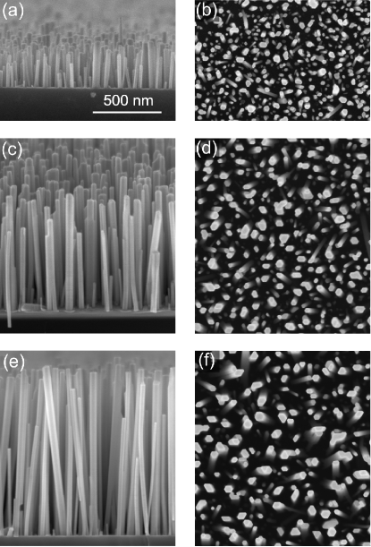
Figure 1: Bird’s eye view (left column) and top-view (right column) scanning electron micrographs of samples 1 (a,b), 2 (c,d), and 3 (e,f). The average NW lengths are 230, 650, and 985 nm, respectively. The scale bar in (a) is applicable to all micrographs.

Figure 1 presents scanning electron micrographs of samples 1–3. Sample 1 corresponds to the end of the NW nucleation process. The NW density is $3.5\times 10^{10}$ cm^-2, while the average length and diameter of the NWs are 230 and 22 nm, respectively. The NWs are mostly uncoalesced hexagonal prisms. Samples 2 and 3 display the further growth of the NWs, with average NW lengths of 650 nm for sample 2 and 985 nm for sample 3. The average NW diameters, as determined by the analysis of the top-view micrographs (right column of Fig. 1), increase with increasing NW lengths, while the NW density decreases. kaganer16bundling showed that the increase in the diameter is a result of NW bundling, rather than their radial growth. A decisive proof of the absence of radial growth comes from the measurement of the fraction of the total area that is covered by NWs. The area fraction covered by the NWs, derived from the top-view micrographs shown in the right column of Fig. 1, does not change from one sample to the other and remains always at 20%.

The distribution of the NW orientations was determined with a laboratory X-ray diffractometer. We have measured the full width at half-maximum (FWHM) of the GaN 0002 reflection to determine the tilt range with respect to the substrate surface normal and the GaN $1\bar{1}00$ reflection to determine the twist range with respect to the in-plane orientation of the substrate. The FWHM of the tilt distribution is found to decrease with the NW length from 5.1 ^∘ for sample 1 to 4.0 ^∘ and 3.9 ^∘ for samples 2 and 3, respectively, as a consequence of bundling. The FWHM of the twist distribution is found to be 2.8 ^∘, 2.7 ^∘, and 3.1 ^∘ for samples 1, 2, and 3, respectively.

The GISAXS measurements were performed at the beamline ID10 of the European Synchrotron Radiation Facility (ESRF) using an X-ray energy of 22 keV (wavelength $\lambda=0.5636\,\textrm{\r{A}}).$ The incident beam was directed at grazing incidence to the substrate. The chosen grazing incidence angle was 0.2 ^∘, i. e., about 2.5 times larger than the critical angle of the substrate, to avoid possible complications of the scattering pattern typical for grazing incidence X-ray scattering [renaud09]. A two-dimensional detector Pilatus 300K (Dectris) placed at a distance of 2.38 m from the sample provided a resolution of $8.06\times 10^{-3}$ nm^-1.

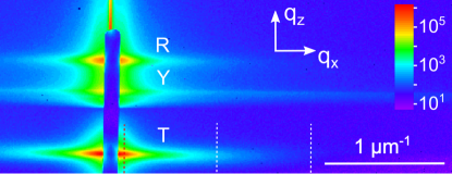
Figure 2: GISAXS intensity from sample 1 as measured by a two-dimensional detector. The scattering around the transmitted beam, the scattering around the beam reflected from the substrate surface, and the Yoneda streak are labeled as T, R, and Y, respectively. The vertical blue bar in the middle of the scattering pattern is the beamstop. The three vertical dotted lines mark the positions of the scans presented in Fig. 3. The color-coded scale bar represents the intensity in counts.

Figure 2 shows the GISAXS intensity measured from sample 1. The scattering pattern comprises three horizontal streaks. The small-angle scattering around the transmitted beam is labeled as “T”, while the scattering around the beam reflected from the substrate surface is labeled as “R”. Both streaks reveal the same scattering intensity dependence on the lateral wavevector $q_{x}$. The scattering around the transmitted beam possesses larger intensity. For that reason, the T streaks is chosen here for the further analysis. Besides the T and R streaks, the intensity distribution in Fig. 2 contains the Yoneda streak, marked with “Y”, which is located at the critical angle for total external reflection. The chosen incidence angle allows us to separate well the three different streaks, which facilitates the analysis of the GISAXS intensity in the framework of kinematical scattering.

3 Analysis of the measured intensities

We use the specific features of the NWs as oriented long prisms to improve the accuracy of the determination of the GISAXS intensity $I(q_{x})$ from the measured maps. Since a single NW is a needle-like object, its scattering intensity in the reciprocal space concentrates in the plane perpendicular to the long axis of the NW. A random tilt of a NW results in the respective tilt of the intensity plane. Hence, one can expect that the spread of 4–5 ^∘ in the directions of the long axes of the NWs results in a sector of intensity in Fig. 2 with the width $\Delta q_{z}$ increasing proportional to $q_{x}$.

Figure 3 presents intensity profiles along the dotted lines indicated in Fig. 2, i.e., scans at constant values of $q_{x}$. These profiles are fitted by a Gaussian plus a background that may linearly depend on $q_{z}$. The FWHMs of these profiles $\Delta q_{z}$ are plotted in Fig. 4(a). As expected, $\Delta q_{z}$ linearly increases with $q_{x}$. The slopes $\Delta q_{z}/q_{x}$ give the angular ranges of the NW orientations to be 5.9 ^∘, 5.1 ^∘, and 4.6 ^∘ for samples 1, 2, and 3, respectively. These values are close to (albeit somewhat larger) the widths of the orientational distributions measured by Bragg diffraction, as described in Sec. 2.

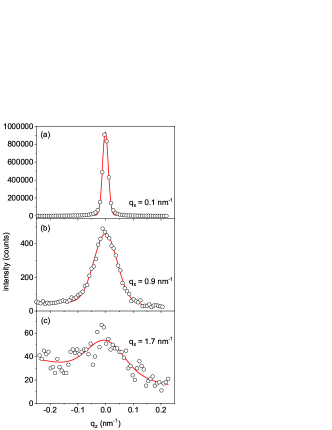
Figure 3: Measured intensity profiles along the lines of constant $q_{x}$ values marked by dotted lines in Fig. 2 (circles) and the respective Gaussian fits (lines).

The fits in Fig. 3 help to improve the determination of the scattering intensity $I(q_{x})$ both at small and large momenta $q_{x}$. At small $q_{x}$, the intensity profiles are narrow and the peak intensity has to be determined from just a few data points. At large $q_{x}$, the intensity is low and the background is comparable to the signal. After performing the fits of the cross-sectional profiles (i.e., along the $q_{z}$ direction) shown in Fig. 3 and establishing the linear dependence of the FWHM $\Delta q_{z}$ on $q_{x}$, we make one more step to improve the accuracy. Linear fits are made for the $\Delta q_{z}$ on $q_{x}$ dependencies plotted in Fig. 4(a). Then, the fits of the $q_{z}$ profiles shown in Fig. 3 are repeated, now with the FWHMs fixed at the values obtained from the linear fits. In this way, the number of free parameters in the Gaussian fits is decreased, and the intensity $I(q_{x})$ is determined more accurately. This intensity is used in the further analysis.

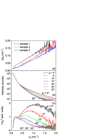
Figure 4: (a) FWHMs of the intensity profiles $\Delta q_{z}$ as a function of the wave vector $q_{x}$. (b) GISAXS intensity profiles of sample 1 as a function of the wave vector $q_{x}$ in dependence of the azimuthal orientation $\psi$. (c) The same intensity profiles as in (b) but plotted as $I(q_{x})q_{x}^{4}$ versus $q_{x}$.

Figure 4(b) presents the GISAXS intensity $I(q_{x})$ measured on sample 1 in dependence on its azimuthal orientation $\psi$. The sample orientation $\psi=0$ corresponds to the incident X-ray beam along a GaN$\left\langle 11\bar{2}0\right\rangle$ direction, so that the scattering vector (the $x$-axis direction) is along $\left\langle 1\bar{1}00\right\rangle$, which is the normal to the NW facets. Figure 4(b) comprises the measurements obtained on the rotation of sample 1 about the normal to the substrate surface (i.e., about the direction of the long axes of the NWs) from $\psi=0\,^{\circ}$ to 30 ^∘ with a step of 5 ^∘. Since the sample has a rectangular shape and the illuminated area varies on rotation, the curves are scaled to obtain the same intensity in the small-$q_{x}$ range. The scaling factors differ less than by a factor of 2. The azimuthal dependence of the intensity at large $q_{x}$ is evident from the plot.

In the case of the reflected beam (the streak “R” in Fig. 2), an identical analysis of the intensity (not shown here) results in curves close to those shown in Fig. 4(b). Thus, we observe the same azimuthal dependence of the intensity but with a smaller total intensity and a higher level of noise. Because of this reason, for the further analysis presented in the paper, we exclusively consider the intensity distributions around the transmitted beam.

Since we expect Porod’s law $I(q_{x})\sim q_{x}^{-4}$ to be satisfied at large $q_{x}$, we plotted in Fig. 4(c) the same data as $I(q_{x})q_{x}^{4}$ versus $q_{x}$, which would tend to a constant value for large $q_{x}$. Surprisingly, a strong deviation from Porod’s law is observed. Furthermore, the data do not only deviate from Porod’s law, but also exhibit a strong azimuthal dependence. In other to explain this unexpected behavior, in the next section, we develop a Monte Carlo method to calculate the scattering intensity.

4 Calculation of the scattering intensity

4.1 Scattering amplitude of a prism

We calculate first the scattering amplitude (form factor) of a NW $A(\mathbf{q})$ in a coordinate system linked to the NW, i.e., with $z$-axis in the direction of the long axis of the NW. Hence, the cross-section of the NW is in the $xy$ plane. Next, we will consider in Sec. 4.3 a transformation of the wave vectors from the laboratory frame to the NW coordinate system, and perform an average of the intensities $\left|A(\mathbf{q})\right|^{2}$ over different NW orientations.

The scattering amplitude of a NW is given by its form factor

$$A(\mathbf{q})=\int_{V}\exp(i\mathbf{q}\cdot\mathbf{r})\,\mathrm{d}\mathbf{r},$$ (1)

where the integral is calculated over the NW volume $V$. Since the NW is a prism, the scattering amplitude can be represented as a product of the components along the NW axis and in the plane perpendicular to it, $A(\mathbf{q})=A_{\parallel}(q_{\parallel})A_{\perp}(\mathbf{q_{\perp}})$. The longitudinal component is simply

$$A_{\parallel}(q_{\parallel})=\mathrm{sinc}(q_{\parallel}L/2),$$ (2)

where $\mathrm{sinc}(x)=(\sin x)/x$ and $L$ is the NW length.

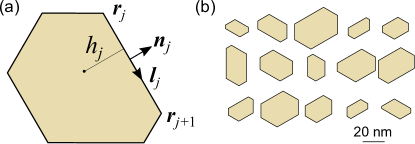
Figure 5: (a) A hexagon with vertices $\mathbf{r}_{j}$ and the unit vectors along and normal to the side $\mathbf{l}_{j}$ and $\mathbf{n}_{j}$. The distance from the hexagon center to its side is $h_{j}$. (b) Examples of randomly generated hexagons used to simulate the scattering from sample 1.

The calculation of the transverse component $A_{\perp}(\mathbf{q_{\perp}})$ can be reduced to a sum over the vertices, as it was initially shown for faceted crystals by laue36 and used nowadays to calculate form factors of nanoparticles [vartanyants08, renaud09, pospelov20]. Specifically, laue36 proposed to reduce, using Gauss’ theorem, the volume integral (1) to the integrals over the facets; application of Gauss’ theorem to these area integrals reduces them to integrals over the edges, which, in turn, can be taken by parts and expressed through the coordinates of the vertices.

For a planar polygon, the form factor reads

$$A_{\perp}(\mathbf{q_{\perp}})=\frac{1}{q_{\perp}^{2}}\sum_{j}\frac{\mathbf{q}_{\perp}\cdot\mathbf{n}_{j}}{\mathbf{q}_{\perp}\cdot\mathbf{l}_{j}}\left(e^{i\mathbf{q}_{\perp}\cdot\mathbf{r}_{j+1}}-e^{i\mathbf{q}_{\perp}\cdot\mathbf{r}_{j}}\right),$$ (3)

where the sum runs over the vertices and, as illustrated in Fig. 5(a), $\mathbf{r}_{j}$ are coordinates of the vertices, $\mathbf{l}_{j}$ and $\mathbf{n}_{j}$ are unit vectors along the polygon side between the vertices $\mathbf{r}_{j}$ and $\mathbf{r}_{j+1}$ and normal to it, respectively. lee83 proposed another expression for the form factor,

$$A_{\perp}(\mathbf{q_{\perp}})=\sum_{j}e^{i\mathbf{q}_{\perp}\cdot\mathbf{r}_{j}}\frac{\left(\mathbf{l}_{j}\times\mathbf{l}_{j-1}\right)\cdot\mathbf{N}}{\left(\mathbf{q}_{\perp}\cdot\mathbf{l}_{j}\right)\left(\mathbf{q}_{\perp}\cdot\mathbf{l}_{j-1}\right)},$$ (4)

where $\mathbf{N}$ is the unit vector normal to the polygon plane, and wuttke17 explicitly showed the identity of the expressions (3) and (4). Equation (3) makes it possible to easily resolve the numerical uncertainty $0/0$ that arises at $\mathbf{q}_{\perp}\cdot\mathbf{l}_{j}=0$. Since $\mathbf{l}_{j}=\left(\mathbf{r}_{j+1}-\mathbf{r}_{j}\right)/\left|\mathbf{r}_{j+1}-\mathbf{r}_{j}\right|$, we have in the limit $\mathbf{q}_{\perp}\cdot\mathbf{l}_{j}\rightarrow 0$

$$\frac{1}{\mathbf{q}_{\perp}\cdot\mathbf{l}_{j}}\left(e^{i\mathbf{q}_{\perp}\cdot\mathbf{r}_{j+1}}-e^{i\mathbf{q}_{\perp}\cdot\mathbf{r}_{j}}\right)\rightarrow ie^{i\mathbf{q}_{\perp}\cdot\mathbf{r}_{j}}\left|\mathbf{r}_{j+1}-\mathbf{r}_{j}\right|.$$ (5)

Figure 6(a) shows the intensity distribution calculated by Eq. (3) for a regular hexagon with a side length of 12 nm. The intensity is higher in the directions of the side normals and oscillates due to interference from opposite sides of the hexagon. Figure 6(b) shows a Monte Carlo calculation of the average intensity from hexagons of different sizes. A lognormal distribution of the lengths of the hexagon sides is taken with the same mean value of 12 nm and a standard deviation of 4 nm.

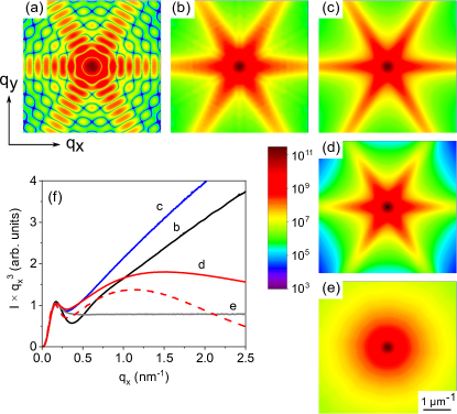
Figure 6: Scattering intensity from (a) a regular hexagon with a side length of 12 nm, (b) a distribution of regular hexagons with the average side length of 12 nm and a standard deviation of the side lengths of 4 nm, (c) a distribution of distorted hexagons as shown in Fig. 5(b), (d) the same distribution as in (c) but with a side facet roughness $\sigma=0.6$ nm added according to Eq. (7), (e) a distribution of randomly oriented distorted hexagons. The color-coded scale bar representing the intensity is applicable to (a)–(e). (f) Radial intensity distributions from (b)–(e) in the directions of the intensity maxima, the product $Iq^{3}$ is plotted. The curves are labeled by the same symbols as the respective maps. The effect of roughness is illustrated in (f) by two curves: the full red curve corresponds to the geometric distribution of the atomic steps on the side facets and the dashed red curve to the Poisson distribution, both possessing the same rms roughness of $\sigma=0.6$ nm.

The radial intensity distribution in the direction along the intensity maximum is presented in Fig. 6(f) by the black line. The intensity distribution is presented as the product $Iq_{x}^{3}$, which would be constant at large $q_{x}$ for an ensemble of randomly oriented hexagons (as well as for other two-dimensional objects with rigid boundaries) after averaging over all possible orientations. As stated above, the intensity maxima in Fig. 6(b) correspond to the directions normal to the sides of the hexagon. They possess, at large $q_{x}$, a $I\propto q_{x}^{-2}$ dependence due to a steplike variation of the density at a planar surface. Hence, in Fig. 6(f), we observe a linear increase of the intensity for large values of $q_{x}$ (black line).

The local maximum at $q_{m}=0.175$ nm^-1 in Fig. 6(f) is related to the mean length of the side facet of the hexagons $a=12$ nm as $a\approx 2.1/q_{m}$, which allows us to determine the hexagon size directly from the plots of $Iq_{x}^{3}$ versus $q_{x}$ (in the three-dimensional case of hexagonal prisms, the same formula is applicable for the maximum in $Iq_{x}^{4}$ versus $q_{x}$ plot, see Sec. 4.3). For comparison, the form factor of a circle of radius $R$ gives $I(q)q^{3}\propto J_{1}^{2}(qR)$, where $J_{1}(x)$ is the Bessel function. The first maximum of $J_{1}(x)$ at $x\approx 1.84$ gives the circle radius $R\approx 1.84/q_{m}$. We can relate a hexagon and a circle even closer, by defining an effective radius $R_{a}$ of a circle possessing the same area as the hexagon with a side length $a$. Then, we have $R_{a}=(3\sqrt{3}/2\pi)^{1/2}a\approx 0.91a$ and $R_{a}\approx 1.9/q_{m}$, with the proportionality coefficient very close to the case of a circle.

With the form factor defined by the positions of the vertices according to either Eq. (3) or Eq. (4), we are not restricted to regular hexagons but can take into account the real cross-sectional shapes of the NWs. Since the side facets of the NWs are GaN{$1\bar{1}00$} planes making an angle of 60 ^∘ to each other, we build the hexagons as shown in Fig. 5(a): random heights $h_{j}$ are taken in the directions normal to the facets. Then, we check that the generated hexagon is convex, and discard it otherwise. Figure 5(b) presents examples of randomly generated hexagons with the same orientation of their sides. The distribution of the hexagon shapes is chosen to simulate sample 1 and further described in Sec. 5. The intensity map obtained from this distribution of hexagons is shown in Fig. 6(c). The respective radial intensity distribution is presented in Fig. 6(f) by the blue line. One can see that the black and the blue lines in Fig. 6(f) are remarkably different. In particular, the hexagon shape distribution notably reduces the dip in the intensity. Therefore, the distortion of the hexagons can be deduced from the intensity plots.

4.2 Roughness of the side facets

The side facets of GaN NWs are atomically flat [stoica08, ristic08] but may have atomic steps. The radial growth of these NWs presumably proceeds by step flow, with the motion of steps from the NW top, where they are nucleated, down along the side facets [garrido13]. Random steps across the side facets can be treated as facet roughness in the same way as it is done in the calculation of crystal truncation rods [Robinson1986a, robinson92].

A step of height $d_{0}$ shifts the $j$th side of the polygon in Fig. 5 by a vector $d_{0}\mathbf{n}_{j}$ in the direction of the facet normal. Hence, the $j$th term in the sum (3) acquires an additional factor $\exp\left(id_{0}\mathbf{q}_{\perp}\cdot\mathbf{n}_{j}\right)$. Random steps give rise to a factor $R_{j}=R(\mathbf{q}_{\perp}\cdot\mathbf{n}_{j})$, where the function $R(q)$ is defined as

$$R(q)=\sum_{m=0}^{\infty}p_{m}\exp\left(imqd_{0}\right),$$ (6)

here $p_{m}$ are the probabilities of the shift of the side facet by $m$ steps. Hence, the function $R(q)$ is the characteristic function of the probabilities $p_{m}$.

Consider the geometric probability distribution $p_{m}=(1-\beta)\beta^{m}$ with the parameter $\beta<1$. It describes a flat surface with a fraction $\beta$ one step higher, its fraction $\beta$ is, in turn, one step higher, and so on [Robinson1986a]. The root mean squared (rms) roughness is $\sigma=d_{0}\sqrt{\beta}/(1-\beta)$ and the corresponding characteristic function is

$$R(q)=\frac{1-\beta}{1-\beta\exp(iqd_{0})}.$$ (7)

The Poisson probability distribution $p_{m}=\exp(-\mu)\mu^{m}/m!$ gives rise to the rms roughness $\sigma=d_{0}\sqrt{\mu}$ and the characteristic function is

$$R(q)=\exp\left[-\mu\left(1-e^{iqd_{0}}\right)\right].$$ (8)

We stress here that the $j$th term in the sum (3) is multiplied with a complex factor $R_{j}=R(\mathbf{q}_{\perp}\cdot\mathbf{n}_{j})$ that depends on the orientation of the respective facet. This is different from a common treatment of the surface roughness, which involves a single factor $\left|R\right|^{2}$. Particularly, the Poisson probability distribution gives for $qd_{0}\ll 1$ the factor $\left|R\right|^{2}=\exp\left(-\sigma^{2}q^{2}\right)$. buttard13 used such a factor to describe the effect of the roughness on the scattered intensity from Si NWs, by analogy to the roughness of planar surfaces, and arrived at an rms roughness $\sigma$ of 1 nm for their samples. We use Eq. (3) in further calculations with the complex factors $R_{j}$ in each term of the sum.

Figure 6(d) shows the scattering intensity distribution obtained with the roughness factors given by Eq. (7). The rms roughness is taken to be $\sigma=0.6$ nm and the step height $d_{0}$ is that of the atomic steps on the GaN($1\bar{1}00$) facet, $d_{0}=a_{0}\sqrt{3}/2$, where $a_{0}=0.319$ nm is the GaN lattice spacing. Strictly speaking, the roughness factors given by Eq. (7) or Eq. (8) are derived for a prism which has in each cross-section a hexagon with straight sides. It describes a variation of the cross-section of the prism along its length and does not make sense for two-dimensional objects. Hence, the intensity distribution shown in Fig. 6(d) corresponds to the prisms with perfectly aligned long axes.

The solid red line in Fig. 6(f) shows the radial intensity distribution obtained from the map shown in Fig. 6(d) in the direction of maximum intensity, calculated using the roughness factors for the geometric probability distribution given by Eq. (7). The dashed red line in Fig. 6(f) shows the intensity from the same distribution of hexagons but calculated using the roughness factors derived from the Poisson probability distribution, Eq. (8). The rms roughness is taken the same in both cases, $\sigma=0.6$ nm. One can see that the roughness qualitatively changes the intensity at $q\sigma>1$. Hence, the rms roughness $\sigma$ can be obtained from the intensity plots. Moreover, the intensity curves are fairly sensitive to the choice of the probability distribution. The crystal truncation rods from planar surfaces possess a similar sensitivity to the choice of the roughness model [walko00]. Our modeling of the scattering from GaN NWs presented in Sec. 5 shows that the geometric probability distribution provides a better agreement with the experimental data.

4.3 Orientational distribution of the NWs

The scattering intensity is measured as a function of the wave vector $\mathbf{q}$ in the laboratory frame (see Fig. 2). We need to find the components $(q_{\parallel},\mathbf{q}_{\perp})$ of this vector in the frame given by the long axis of the NW and the normal to one of its side facets. Let us consider first the simple case of the two-dimensional rotation of the hexagons (or perfectly aligned prisms in the plane normal to their long axes). The unit vector normal to a hexagon side (or the prism facet) can be written as

$$\mathbf{n}=(\cos\psi,\sin\psi,0),$$ (9)

where $\psi$ is a polar angle (defined modulo 60 ^∘) with respect to a reference orientation. The unit vector along the hexagon side is, respectively, $\mathbf{l}=(-\sin\psi,\cos\psi,0)$. The components $q_{n}$, $q_{l}$ of the two-dimensional vector $\mathbf{q}_{\perp}$ are determined simply as $q_{n}=\mathbf{q_{\perp}}\cdot\mathbf{n}$ and $q_{l}=\mathbf{q_{\perp}}\cdot\mathbf{l}$.

Figure 6(e) presents a Monte Carlo calculation of the intensity for the distribution of distorted hexagons described above and sketched in Fig. 5(b), after an average over the orientations $\psi$ uniformly distributed from 0 ^∘ to 360 ^∘. The corresponding radial intensity distribution, shown in Fig. 6(f) by a gray line, follows the two-dimensional Porod’s law $I(q)\propto q^{-3}$ at large $q$. At small $q$, it coincides with the intensity distribution for the oriented hexagons.

For the three-dimensional distribution of the NW orientations, inherent to the spontaneous formation of GaN NWs on Si(111) (see Fig. 1), we define a unit vector in the direction of the long NW axis as

$$\mathbf{e}_{\parallel}=(\sin\theta\cos\phi,\sin\theta\sin\phi,\cos\theta),$$ (10)

where $\phi$ and $\theta$ are the azimuthal angle of tilt and its polar angle, respectively. The unit vector normal to the facet is defined to be orthogonal to $\mathbf{\mathbf{e}_{\parallel}}$ and possessing the same projection on the horizontal plane as in Eq. (9):

$$\mathbf{n}=(\xi\cos\psi,\xi\sin\psi,s\sqrt{1-\xi^{2}}),$$ (11)

where $\xi=\left[1+\tan^{2}\theta\cos^{2}\left(\phi-\psi\right)\right]^{-1/2}$ and $s$ is the sign of $-\cos\left(\phi-\psi\right)$. Since the tilt angle $\theta$ does not exceed a few degrees, the difference between Eqs. (9) and (11) is unessential. The vector $\mathbf{l}$ is defined as a vector product $\mathbf{l}=\mathbf{e}_{\parallel}\times\mathbf{n}$.

We calculate the scattering intensity by the Monte Carlo method. It enables a simultaneous integration over the distributions of the NW lengths, their cross-sectional sizes and shapes, and the orientations of the NW long axis as well as those of their side facets. The calculations take fairly little time. It takes less than a minute on a single CPU core of a standard PC to calculate an intensity curve with the accuracy sufficient to make estimates. The smooth curves presented in the paper took less than an hour of CPU time each.

We take the mean NW lengths obtained from the scanning electron micrographs and given in Sec. 2. A large scattering in the NW lengths is evident from Fig. 1. The length distribution is assumed to be lognormal with a standard deviation of 20% from the respective average lengths. For the facet orientation angle $\psi$, we take a normal distribution with the FWHM determined by the in-plane X-ray diffraction scans (see Sec. 2). The average value of $\psi$ is given by the orientation of the incident X-ray beam with respect to the NW facets [see Figs. 4(b) and 4(c)].

The integration over the orientations of the long axis of the NWs is an integration over a solid angle, i.e., the integral of the intensity from a single NW with $P(\theta)\sin\theta\,\mathrm{d}\theta\mathrm{d}\phi$, where $P(\theta)$ is the probability density distribution of the tilt angle $\theta$. The azimuthal angle $\phi$ is uniformly distributed from 0 to $2\pi$. We take a normal distribution of the tilt angles, $P(\theta)=\sqrt{2/\pi}(\Delta\theta)^{-1}\exp[-\theta^{2}/2(\Delta\theta)^{2}]$. The standard deviation $\Delta\theta$ can be obtained from the slopes of the straight lines in Fig. 4(a) or from the FWHMs of the symmetric Bragg reflections GaN 0002, as discussed in Sec. 3. The widths $\Delta q_{z}$ in Fig. 4(a) and the FWHMs of the Bragg reflections take into account the tilts in all directions, so that $\Delta\theta$ is obtained from the half width at half maximum (HWHM) and varies from 2.5 ^∘ for sample 1 to 2 ^∘ for sample 3. Since the tilt angle $\theta$ is small, we can take $\sin\theta\approx\theta$ and proceed to an integral over a new variable $y=\theta^{2}$. Then, the integral is taken with $\tilde{P}(y)\,\mathrm{d}y\mathrm{d}\phi$, where $\tilde{P}(y)\propto\exp[-y/2(\Delta\theta)^{2}]$. Hence, we generate $y$ as an exponentially distributed random number with the unit dispersion and calculate $\theta=\sqrt{2y}\Delta\theta.$

If the NW orientations are completely random, i.e., the angles $\phi$ and $\psi$ vary from 0 to $2\pi$ and the angle $\theta$ from 0 to $\pi$ uniformly and independently, the small-angle scattering intensity at $q\gg 2\pi/a$, where $a$ is the width of the side facet, follows Porod’s law $I(q)\propto q^{-4}$. However, since the NWs are long prisms, the scattering intensity from a single NW of length $L$ with its long axis in $z$-direction concentrates in the reciprocal space in a disk of the width $\Delta q_{z}=2\pi/L$. We have seen in Sec. 3 that the scattering from the oriented NWs is limited by $\Delta q_{z}/q_{x}<\Delta\theta$, where $\Delta\theta$ is the angular range of orientations. As long as $2\pi/(Lq_{x})<\Delta\theta$, the oriented NWs give the same intensity in the $x$-direction as fully randomly oriented ones. Therefore, Porod’s law is satisfied for $q_{x}>2\pi/(L\Delta\theta)$.

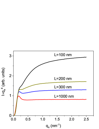
Figure 7: Monte Carlo calculation of the small-angle scattering intensity from an ensemble of NWs with a 5 ^∘ wide range of orientations of the long axes and random orientation of the side facets. The width of the side facets is 12 nm and NW lengths vary from 100 to 1000 nm.

Figure 7 presents the Monte Carlo calculation of the small-angle scattering intensity from NWs of different lengths and the same width of the tilt angle distribution $\Delta\theta=2.5\,^{\circ}$ corresponding to that of sample 1. Particularly, for the NWs with a length $L=200$ nm, the condition derived above reads $q_{x}>0.7$ nm^-1, which is in a good agreement with the region of constant $I(q_{x})q_{x}^{4}$ in Fig. 7. Hence, the limited range of the tilt angles in the NW ensemble does not prevent reaching Porod’s law even for the relatively short NWs of sample 1. We remind that the curves in Fig. 7 are calculated by averaging over the tilt azimuth $\phi$ and the facet orientation $\psi$ varying from 0 to $2\pi$. Further Monte Carlo calculations, taking into account the orientational ordering of the side facets of the epitaxially grown GaN NWs, are presented in the next section.

5 Results

Figure 8 presents the results of the systematic GISAXS measurements on samples 1–3. The measurements and their analysis are described in the sections 2 and 3, respectively. The samples have been measured with the azimuthal orientation $\psi$ varying from 0 ^∘ to 90 ^∘ with steps of 5 ^∘. Each measurement provided a map similar to the one in Fig. 2, and the intensity $\mathcal{I}(q_{x},q_{z})$ around the transmitted beam has been analyzed by fitting every scan of a constant $q_{z}$ by a Gaussian, as shown in Fig. 3. The peak values of the $q_{z}$ scans obtained in this fit provided the intensity $I(q_{x})$. It is presented in Fig. 8 as the product $I(q_{x})q_{x}^{4}$ versus $q_{x}$, to reveal deviations from Porod’s law.

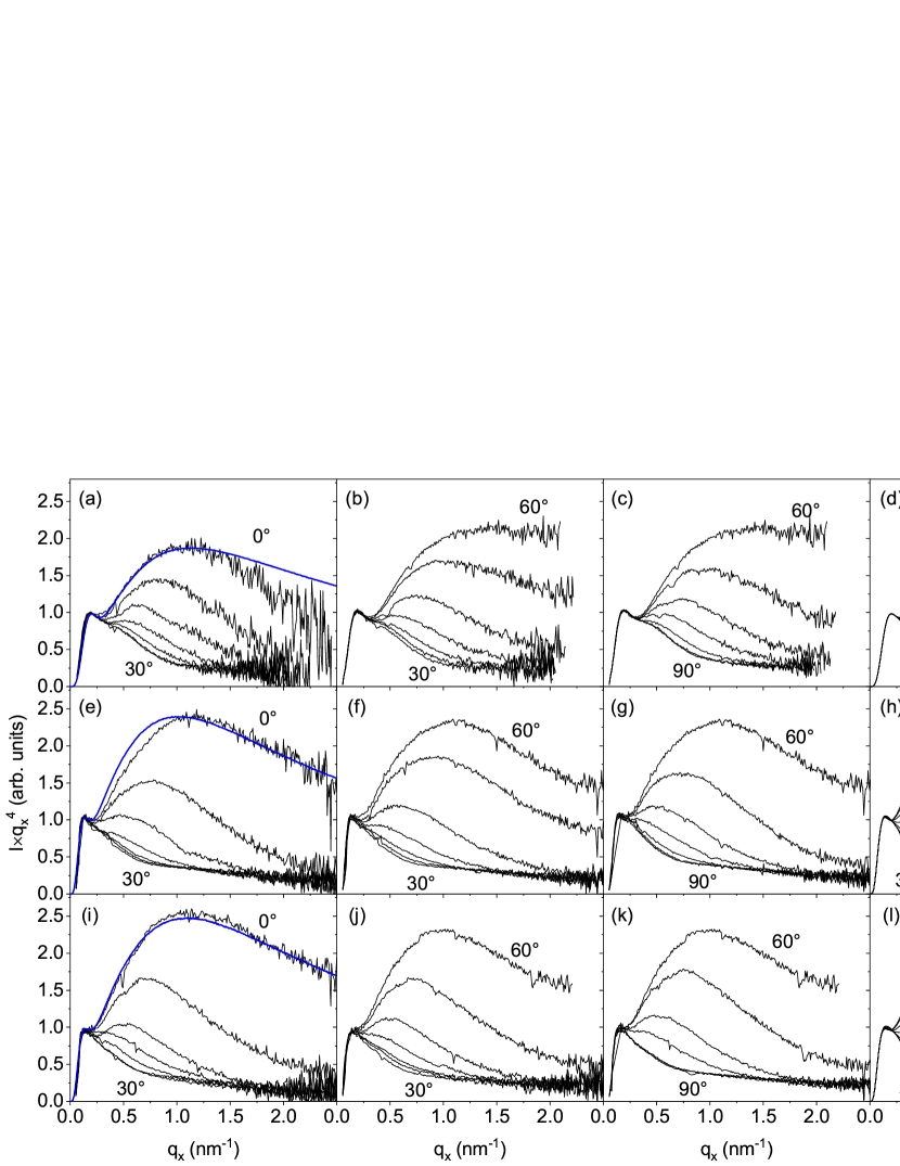
Figure 8: The measured GISAXS intensity (three left columns) and Monte Carlo simulations (right column) for samples 1 (a–d), 2 (e–h), and 3 (i–l). The measurements are performed for different mean orientation angles $\psi$ of the side facets of the NWs with respect to the X-ray beam, namely, from 0 ^∘ to 90 ^∘ with steps of 5 ^∘. For clarity, these measurements are presented in three different panels (from 0 ^∘ to 30 ^∘, from 30 ^∘ to 60 ^∘, and from 60 ^∘ to 90 ^∘). The intensities are plotted as $I(q_{x})q_{x}^{4}$ versus $q_{x}$ to highlight deviations from Porod’s law. The curves calculated at $\psi=0^{\circ}$ for each sample are repeated as blue curves in the left column, for a direct comparison of the calculated and the measured curves.

Since GaN NWs grow epitaxially on Si(111), the ensemble possesses a 6-fold orientational symmetry. A systematic variation of the intensity curves depending on the azimuthal sample orientation $\psi$ is evident from Fig. 8: within the statistical error of the measurements, the orientations $\psi$ and $\psi+60\,^{\circ}$, as well as $\pm\psi$ or $30\,^{\circ}\pm\psi$, are equivalent. Hence, the Monte Carlo modeling presented in the right column of Fig. 8 has been performed for the angle $\psi$ from 0 ^∘ to 30 ^∘ with the same step of 5 ^∘.

In the Monte Carlo calculations, we take the values of the NW lengths $L$, the range of the tilt angles $\theta$, and the range of the side facet orientations $\psi$ at the values experimentally determined in Secs. 2 and 3. The parameters of the NW ensemble to be determined from the modeling are the mean width of the side facets $a$, its variation as well as the variation of the cross-sectional shapes of the NWs, and the roughness of the side facets. We have seen in Sec. 3 that these parameters affect the calculated curves in qualitatively different ways. The mean facet size $a$ determines the position of the local maximum of the curves at $q_{x}\approx 0.17$ nm^-1, which corresponds to a side facet width of about 12 nm. The depth of the dip between this maximum and the rise of the curves at larger $q_{x}$ is controlled by the width of the facet size distribution and the shape distribution of the cross-sections. The decrease of $Iq_{x}^{4}$ at large $q_{x}$ is caused by the roughness of the side facets.

The distorted cross-sections of the NWs are modeled in the Monte Carlo study as described in Sec. 4.1. The heights $h_{j}$ shown in Fig. 5(a) are generated on random around a mean value. Figure 5(b) exemplifies the shapes of the NWs used in the simulation of sample 1. The right column in Fig. 8 presents the Monte Carlo calculation of the small-angle scattering intensity for samples 1–3. For a direct comparison of the calculated and the measured intensities, the curves calculated for each sample at $\psi=0{}^{\circ}$ are repeated as blue lines in the left column of the figure.

For each generated NW, we calculate the cross-sectional area $A$ and the perimeter $P$. Then, we determine out of these parameters the radius $R$ from $A=\pi R^{2}$ and the circularity $C=4\pi A/P^{2}$. The circularity thus defined is $C=1$ for a circle, $C=\pi\sqrt{3}/6\approx 0.907$ for a regular hexagon, and $C\ll 1$ for irregular shapes. These parameters, radius and circularity, can be obtained from scanning electron micrographs and are objective NW shape descriptors as discussed elsewhere [brandt14]. The lines in Fig. 9 show the distributions of the radius and the circularity obtained in the simulations.

The distributions of the cross-sectional radii and circularities of the NW ensembles have also been interdependently obtained by analyzing top-view scanning electron micrographs similar to those shown in Fig. 1(d–f). The analysis has been performed using the open-source software ImageJ [schneider12], as described in detail by kaganer16bundling in their Supporting Information. The distribution of the radius obtained from the modeling of the GISAXS intensity for sample 1 in Fig. 9(a) is fairly close to the distribution derived from the micrographs. The circularity distribution obtained from the micrographs is, however, extended towards smaller values indicating a higher density of NWs with elongated cross-sectional shapes. Such a discrepancy can be attributed to an artifact caused by the NW tilt. Specifically, the scanning electron micrographs exhibit a very little difference in brightness between the top facet and the top part of the side facet of the NW, so that ImageJ treats both regions together, i. e., as extended intensity spots.

In contrast to sample 1, the NW radii obtained from the Monte Carlo simulations of the scattering intensity from samples 2 and 3, see Figs. 9(c) and 9(e), are smaller than those derived from the analysis of the scanning electron micrographs, and the discrepancy increases with increasing NW length. We remind that the mean NW radius can be directly derived from the position $q_{x}$ of the local maximum in the experimental curves presented in Fig. 8. It remains at about $q_{x}\approx 0.17$ nm^-1 and only slightly shifts to smaller values (and hence to larger radii) as the NW length increases from sample 1 to sample 3.

The origin of the discrepancy between the NW radii determined from the scanning electron micrographs and from the modeling of the GISAXS intensity is in the bundling of NWs. The bundling is almost absent for sample 1, and the cross-sections of the NWs obtained from the micrographs characterize the NWs along their full length. As the NWs grow in length, they bundle together, which causes an apparent radial growth. Simultaneously, the NW density decreases, so that the fraction of the surface covered by the NWs remains constant [kaganer16bundling]. The GISAXS provides a statistics of the NW radii averaged over their lengths, while the top-view micrographs reveal their distribution at the top. That results in a progressive difference between the distributions obtained by the two methods.

The widths of the circularity distributions in the right column of Fig. 9 slightly reduce with the growth of the NWs. The NW images in the scanning electron micrographs become more circular since, during NW growth, the bundled nanowires attain a common shape that tends to a regular hexagon. Also, the low-circularity wing of the circularity histogram reduces, because the effective radii of the bundled NWs increase, and the distinction between the top facets and the top parts of the side facets becomes more pronounced for the ImageJ analysis. The circularity distributions obtained from the GISAXS intensity curves are sharper than the ones obtained from scanning electron micrographs, because the former takes into account both single NWs in their bottom part and bundled NWs in their top part, while the latter counts only the NW tops. We also remind that the circularity of a distorted hexagon is always smaller than the circularity $C\approx 0.907$ of a regular hexagon. Larger circularities obtained from the analysis of the scanning electron micrographs in Figs. 9(d) and  9(f) are due to the finite resolution of the micrographs as well as to the algorithm used by ImageJ that tends to round faceted objects.

We have seen in Sec. 4.1 and particularly in Fig. 6(f) that, when the scattering vector is oriented normal to the side facets of the NWs ($\psi=0\,^{\circ}$) and the facets are atomically flat, the facet truncation rod scattering would result in a linear increase of the intensity on the $I(q_{x})q_{x}^{4}$ vs. $q_{x}$ plot at large $q_{x}$. The decrease of the experimental curves indicates a roughness of the side facets. We obtain in the Monte Carlo modeling an rms roughness of $\sigma=0.9$, 0.95, and 0.85 nm for samples 1, 2, and 3, respectively. According to the height of the atomic steps on a GaN($1\bar{1}00$) facet $d_{0}=a_{0}\sqrt{3}/2=0.276$ nm (here $a_{0}=0.319$ nm is the GaN lattice spacing), the rms roughness is less than 3.5 steps.

6 Discussion and summary

GaN NWs nucleate spontaneously on Si(111) and grow with a substantial disorder with respect to their orientations. Their growth is, nevertheless, epitaxial: the NWs inherit the out-of-of plane and in-plane orientations of the substrate. Since these NWs are typically long (from hundreds of nanometers to a few microns) and thin (tens of nanometers), the range of orientations of their long axes of 3–5 ^∘ is sufficient to provide the same average in the small-angle scattering intensity as if they would have all orientations. However, an angular range of orientations of the side facets of 3 ^∘ gives rise to features in the GISAXS intensity distribution that are reminiscent of the crystal truncation rod scattering from flat surfaces of single crystals.

We have found that the GISAXS intensity depends on the orientation of the side facets with respect to the incident X-ray beam direction. In our experiment, the incident beam is kept normal to the average direction of the long axes of the NWs. The orientation of the incident beam with respect to the side facets is varied by rotating the sample about the substrate surface normal. The scattering intensity is maximum when the incident beam is along the facets, or in other words, when the scattering vector is in the direction of the facet normal.

The X-ray scattering intensity from a planar surface is proportional to $q^{-2}$. Porod’s law $q^{-4}$ is a result of a full average over all orientations of the plane [sinha88], i.e., the integration over the two angles defining the plane orientation. For GaN NWs on Si(111), the range of orientations of the long axes is large enough to provide an integration over the tilt angle and give rise to a $q^{-3}$ dependence when the scattering vector is along the facet normal. In the $Iq^{4}$ vs. $q$ plots shown in Fig. 8, this dependence is seen as a linear increase at $\psi=0\,^{\circ}$ or $60\,^{\circ}$. The intensity decreases as the sample is rotated about the normal to the substrate surface. The minimum intensity value is reached at $\psi=30\,^{\circ}$, i.e., in the direction between facets.

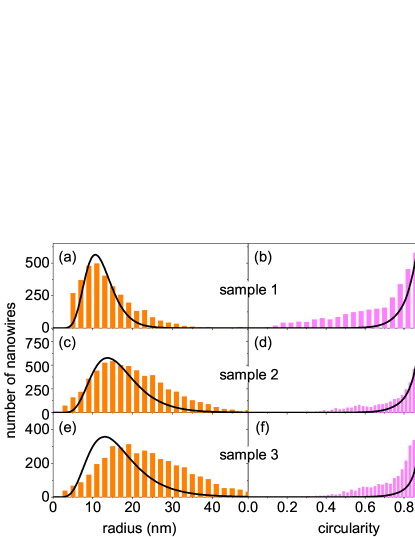
Figure 9: Distributions of the NW radii and circularities of samples 1–3 obtained from the analysis of the top-view scanning electron micrographs (histograms) and the Monte Carlo modeling (lines).

The surface roughness gives rise to a decrease in the intensity at $q\sigma\gtrsim 1$, where $\sigma$ is the rms roughness. The Monte Carlo modeling of the experimental curves in Fig. 8 gives $\sigma$ from 0.85 to 0.95 nm, which is just 3.5 times the height of the atomic steps. Nevertheless, this small roughness strongly modifies the intensity curve for high values of $q$.

The GISAXS curves vary fairly little from one sample to another, despite the large difference between the cross-sectional sizes of the NWs observed in the scanning electron micrographs shown in Fig. 1. This apparent discrepancy is explained by the NW bundling, which is an essential effect in their growth [kaganer16bundling]. While GISAXS reflects the distribution of the cross-sectional sizes of the NWs over their whole volume, the top-view micrographs shown in the right column of Fig. 1 reveals the cross-sectional sizes of the NWs at their very top part. As a result, the distributions of the NW radii and circularities obtained from the scanning electron micrographs and the GISAXS intensity curves only coincide for sample 1, which is free of bundling. As the NWs grow in height and their bundling increases (samples 2 and 3), the discrepancies between the results obtained by these two different methods increases.

Finally, we conclude that GISAXS, together with the Monte Carlo modeling of the intensity curves, is well suited for the determination of the distributions of the cross-sectional sizes of the NWs. The methods developed in the present paper are not specific to GaN NWs on Si(111) and can be applied to other NW distributions and material systems. Particularly, they will be applied in a separate work to the assessment of the radius distributions of GaN NW ensembles grown on TiN, which exhibit a much lower density that hinders the analysis of the NW cross-sectional shapes by scanning electron microscopy.

7 Acknowledgments

We thank Vladimir Volkov (Institute of Crystallography, Moscow) for useful discussions, and Oliver Brandt (Paul-Drude-Insitut, Berlin) for useful discussions and a critical reading of the manuscript, Lewis Sharpnack (ESRF, Grenoble) for his assistance during preliminary measurements at the ESRF beamline ID02, Shyjumon Ibrahimkutty (Rigaku, Neu-Isenburg) for the measurement of the NW twist angles, Carsten Stemmler (Paul-Drude-Institut, Berlin) for his help with the preparation of the samples, and Anne-Kathrin Bluhm (Paul-Drude-Institut, Berlin) for providing the scanning electron micrographs. S.F.-G. acknowledges the partial financial support received through the Spanish program Ramón y Cajal (co-financed by the European Social Fund) under grant RYC-2016-19509 from the former Ministerio de Ciencia, Innovación y Universidades.

References

- [1] \harvarditemBale \harvardand Schmidt1984bale84 Bale, H. D. \harvardand Schmidt, P. W. \harvardyearleft1984\harvardyearright. Phys. Rev. Lett. \volbf53, 596–599.
- [2] \harvarditem[Brandt et al.]Brandt, Fernández-Garrido, Zettler, Luna, Jahn, Chèze \harvardand Kaganer2014brandt14 Brandt, O., Fernández-Garrido, S., Zettler, J. K., Luna, E., Jahn, U., Chèze, C. \harvardand Kaganer, V. M. \harvardyearleft2014\harvardyearright. Cryst. Growth Design, \volbf14, 2246–2253.
- [3] \harvarditem[Buttard et al.]Buttard, Schülli, Oehler \harvardand Gentile2013buttard13 Buttard, D., Schülli, T., Oehler, F. \harvardand Gentile, P. \harvardyearleft2013\harvardyearright. Micro & Nano Lett. \volbf8, 709–712.
- [4] \harvarditemConsonni2013consonni2013pss Consonni, V. \harvardyearleft2013\harvardyearright. Phys. Status Solidi Rapid Res. Lett. \volbf7, 699–712.
- [5] \harvarditem[David et al.]David, Buttard, Schülli, Dallhuin \harvardand Gentile2008david08 David, T., Buttard, D., Schülli, T., Dallhuin, F. \harvardand Gentile, P. \harvardyearleft2008\harvardyearright. Surf. Sci. \volbf2008, 2675–2680.
- [6] \harvarditem[Debye et al.]Debye, Anderson, Jr. \harvardand Brumberger1957debye57 Debye, P., Anderson, Jr., H. R. \harvardand Brumberger, H. \harvardyearleft1957\harvardyearright. J. Appl. Phys. \volbf28, 679–683.
- [7] \harvarditem[Eymery et al.]Eymery, Favre-Nicolin, Fröberg \harvardand Samuelson2009eymery09 Eymery, J., Favre-Nicolin, V., Fröberg, L. \harvardand Samuelson, L. \harvardyearleft2009\harvardyearright. Appl. Phys. Lett. \volbf131911, 94.
- [8] \harvarditem[Eymery et al.]Eymery, Rieutord, Favre-Nicolin, Robach, Niquet, Fröberg, Mårtensson \harvardand Samuelson2007eymery07 Eymery, J., Rieutord, F., Favre-Nicolin, V., Robach, O., Niquet, Y.-M., Fröberg, L., Mårtensson, T. \harvardand Samuelson, L. \harvardyearleft2007\harvardyearright. Nano Lett. \volbf7, 2596.
- [9] \harvarditem[Fernández-Garrido et al.]Fernández-Garrido, Grandal, Calleja, Sánchez-García \harvardand López-Romero2009garrido09 Fernández-Garrido, S., Grandal, J., Calleja, E., Sánchez-García, M. A. \harvardand López-Romero, D. \harvardyearleft2009\harvardyearright. J. Appl. Phys. \volbf106, 126102.
- [10] \harvarditem[Fernández-Garrido et al.]Fernández-Garrido, Kaganer, Hauswald, Jenichen, Ramsteiner, Consonni, Geelhaar \harvardand Brandt2014garrido14 Fernández-Garrido, S., Kaganer, V. M., Hauswald, C., Jenichen, B., Ramsteiner, M., Consonni, V., Geelhaar, L. \harvardand Brandt, O. \harvardyearleft2014\harvardyearright. Nanotechnol. \volbf25, 455702.
- [11] \harvarditem[Fernández-Garrido et al.]Fernández-Garrido, Kaganer, Sabelfeld, Gotschke, Grandal, Calleja, Geelhaar \harvardand Brandt2013garrido13 Fernández-Garrido, S., Kaganer, V. M., Sabelfeld, K. K., Gotschke, T., Grandal, J., Calleja, E., Geelhaar, L. \harvardand Brandt, O. \harvardyearleft2013\harvardyearright. Nano Lett. \volbf13, 3274–3280.
- [12] \harvarditem[Fernández-Garrido et al.]Fernández-Garrido, Kong, Gotschke, Calarco, Geelhaar, Trampert \harvardand Brandt2012garrido12 Fernández-Garrido, S., Kong, X., Gotschke, T., Calarco, R., Geelhaar, L., Trampert, A. \harvardand Brandt, O. \harvardyearleft2012\harvardyearright. Nano Letters, \volbf12, 6119–6125.
- [13] \harvarditem[Heying et al.]Heying, Averbeck, Chen, Haus, Riechert \harvardand Speck2000heying00 Heying, B., Averbeck, R., Chen, L. F., Haus, E., Riechert, H. \harvardand Speck, J. S. \harvardyearleft2000\harvardyearright. J. Appl. Phys. \volbf88, 1855–1860.
- [14] \harvarditem[Horák et al.]Horák, Holý, Staddon, Farley, Novikov, Campion \harvardand Foxon2008horak08 Horák, L., Holý, V., Staddon, C. R., Farley, N. R. S., Novikov, S. V., Campion, R. P. \harvardand Foxon, C. T. \harvardyearleft2008\harvardyearright. J. Appl. Phys. \volbf104, 103504.
- [15] \harvarditem[Jenichen et al.]Jenichen, Brandt, Pfüller, Dogan, Knelangen \harvardand Trampert2011jenichen11 Jenichen, B., Brandt, O., Pfüller, C., Dogan, P., Knelangen, M. \harvardand Trampert, A. \harvardyearleft2011\harvardyearright. Nanotechnol. \volbf22, 295714.
- [16] \harvarditem[Kaganer et al.]Kaganer, Fernández-Garrido, Dogan, Sabelfeld \harvardand Brandt2016akaganer16bundling Kaganer, V. M., Fernández-Garrido, S., Dogan, P., Sabelfeld, K. K. \harvardand Brandt, O. \harvardyearleft2016a\harvardyearright. Nano Lett. \volbf16, 3717–3725.
- [17] \harvarditem[Kaganer et al.]Kaganer, Jenichen \harvardand Brandt2016bkaganer16xray Kaganer, V. M., Jenichen, B. \harvardand Brandt, O. \harvardyearleft2016b\harvardyearright. Phys. Rev. Appl. \volbf6, 064023.
- [18] \harvarditem[Kaganer et al.]Kaganer, Jenichen, Brandt, Fernández-Garrido, Dogan, Geelhaar \harvardand Riechert2012kaganer12NWstrain Kaganer, V. M., Jenichen, B., Brandt, O., Fernández-Garrido, S., Dogan, P., Geelhaar, L. \harvardand Riechert, H. \harvardyearleft2012\harvardyearright. Phys. Rev. B, \volbf86, 115325.
- [19] \harvarditemLee \harvardand Mittra1983lee83 Lee, S.-W. \harvardand Mittra, R. \harvardyearleft1983\harvardyearright. IEEE Trans. Antennas Propag. \volbf31, 99–103.
- [20] \harvarditem[Mariager et al.]Mariager, Lauridsen, Dohn, Bovet, Sørensen, Schlepütz, Willmott \harvardand Feidenhans’l2009mariager09 Mariager, S. O., Lauridsen, S. L., Dohn, A., Bovet, N., Sørensen, C. B., Schlepütz, C. M., Willmott, P. R. \harvardand Feidenhans’l, R. \harvardyearleft2009\harvardyearright. J. Appl. Cryst. \volbf42, 369–375.
- [21] \harvarditem[Mariager et al.]Mariager, Sørensen, Aagesen, Nygård, Feidenhans’l \harvardand Willmott2007mariager07 Mariager, S. O., Sørensen, C. B., Aagesen, M., Nygård, J., Feidenhans’l, R. \harvardand Willmott, P. R. \harvardyearleft2007\harvardyearright. Appl. Phys. Lett. \volbf91, 083106.
- [22] \harvarditemPorod1951porod51 Porod, G. \harvardyearleft1951\harvardyearright. Kolloid Z. \volbf124, 83–114.
- [23] \harvarditem[Pospelov et al.]Pospelov, Van Herck, Burle, Carmona Loaiza, Durniak, Fisher, Ganeva, Yurov \harvardand Wuttke2020pospelov20 Pospelov, G., Van Herck, W., Burle, J., Carmona Loaiza, J. M., Durniak, C., Fisher, J. M., Ganeva, M., Yurov, D. \harvardand Wuttke, J. \harvardyearleft2020\harvardyearright. J. Appl. Cryst. \volbf53, 262–276.
- [24] \harvarditem[Renaud et al.]Renaud, Lazzari \harvardand Leroy2009renaud09 Renaud, G., Lazzari, R. \harvardand Leroy, F. \harvardyearleft2009\harvardyearright. Surf. Sci. Rep. \volbf64, 255–380.
- [25] \harvarditem[Ristić et al.]Ristić, Calleja, Fernández-Garrido, Cerutti, Trampert, Jahn \harvardand Ploog2008ristic08 Ristić, J., Calleja, E., Fernández-Garrido, S., Cerutti, L., Trampert, A., Jahn, U. \harvardand Ploog, K. H. \harvardyearleft2008\harvardyearright. J. Cryst. Growth, \volbf310, 4035–4045.
- [26] \harvarditemRobinson \harvardand Tweet1992robinson92 Robinson, I. \harvardand Tweet, D. \harvardyearleft1992\harvardyearright. Rep. Prog. Phys. \volbf55, 599–651.
- [27] \harvarditemRobinson1986Robinson1986a Robinson, I. K. \harvardyearleft1986\harvardyearright. Phys. Rev. B, \volbf33, 3830–3836.
- [28] \harvarditem[Schneider et al.]Schneider, Rasband \harvardand Eliceiri2012schneider12 Schneider, C. A., Rasband, W. S. \harvardand Eliceiri, K. W. \harvardyearleft2012\harvardyearright. Nature Methods, \volbf9, 671–675.
- [29] \harvarditemSinha1989sinha89 Sinha, S. K. \harvardyearleft1989\harvardyearright. Physica D, \volbf38, 310–314.
- [30] \harvarditem[Sinha et al.]Sinha, Sirota, Garoff \harvardand Stanley1988sinha88 Sinha, S. K., Sirota, E. B., Garoff, S. \harvardand Stanley, H. B. \harvardyearleft1988\harvardyearright. Phys. Rev. B, \volbf38, 2297–2311.
- [31] \harvarditem[Stoica et al.]Stoica, Sutter, Meijers, Debnath, Calarco, Lüth \harvardand Grützmacher2008stoica08 Stoica, T., Sutter, E., Meijers, R. J., Debnath, R. K., Calarco, R., Lüth, H. \harvardand Grützmacher, D. \harvardyearleft2008\harvardyearright. Small, \volbf4, 751.
- [32] \harvarditem[van Treeck et al.]van Treeck, Calabrese, Goertz, Kaganer, Brandt, Fernández-Garrido \harvardand Geelhaar2018treeck18 van Treeck, D., Calabrese, G., Goertz, J., Kaganer, V., Brandt, O., Fernández-Garrido, S. \harvardand Geelhaar, L. \harvardyearleft2018\harvardyearright. Nano Res. \volbf11, 565–576.
- [33] \harvarditem[Vartanyants et al.]Vartanyants, Zozulya, Mundboth, Yefanov, Richard, Wintersberger, Stangl, Diaz, Mocuta, Metzger, Bauer, Boeck \harvardand Schmidbauer2008vartanyants08 Vartanyants, I. A., Zozulya, A. V., Mundboth, K., Yefanov, O. M., Richard, M.-I., Wintersberger, E., Stangl, J., Diaz, A., Mocuta, C., Metzger, T. H., Bauer, G., Boeck, T. \harvardand Schmidbauer, M. \harvardyearleft2008\harvardyearright. Phys. Rev. B, \volbf77, 115317.
- [34] \harvarditemvon Laue1936laue36 von Laue, M. \harvardyearleft1936\harvardyearright. Ann. Phys. \volbf26, 55–68.
- [35] \harvarditemWalko2000walko00 Walko, D. A. \harvardyearleft2000\harvardyearright. Ph.D. thesis, University of Illinois at Urbana-Champaign, Urbana, Illinois.
- [36] \harvarditemWong \harvardand Bray1988wong88 Wong, P.-Z. \harvardand Bray, A. J. \harvardyearleft1988\harvardyearright. J. Appl. Cryst. \volbf21, 786–794.
- [37] \harvarditemWuttke2017wuttke17 Wuttke, J. \harvardyearleft2017\harvardyearright. Form factor (Fourier shape transform) of polygon and polyhendron. ArXiv:1703.00255.
- [38]