document

Flooding dynamics of diffusive dispersion in a random potential

Abstract

We discuss the combined effects of overdamped motion in a quenched random potential and diffusion, in one dimension, in the limit where the diffusion coefficient is small. Our analysis considers the statistics of the mean first-passage time $T(x)$ to reach position $x$, arising from different realisations of the random potential: specifically, we contrast the median $\bar{T}(x)$, which is an informative description of the typical course of the dispersion, with the expectation value $\langle T(x)\rangle$, which is dominated by rare events where there is an exceptionally high barrier to diffusion. We show that at relatively short times the median $\bar{T}(x)$ is explained by a ‘flooding’ model, where $T(x)$ is predominantly determined by the highest barriers which is encountered before reaching position $x$. These highest barriers are quantified using methods of extreme value statistics.

1 Introduction

There are many situations where particles move under the combined influence of thermal diffusion and a static (or quenched) random potential Havlin2002 . The particles might be electrons, holes or excitons diffusing in a disordered metallic or semiconductor sample Cha+95 , or molecules diffusing in a complex environment such as the cytoplasm of a eukaryotic cell Saxton2007 . The state of knowledge of this problem is surprisingly under-developed, and in this work we present new results on the simplest version of this problem, in one dimension, where the equation of motion is

$$\dot{x}=-\frac{{\rm d}V}{{\rm d}x}+\sqrt{2D}\,\eta(t)\ .$$ (1)

Here $V(x)$ is a random potential, $D$ is the diffusion coefficient, and $\eta(t)$ is a white noise signal with statistics defined by

$$\langle{\eta(t)}\rangle=0\ ,\ \ \ \langle\eta(t)\eta(t^{\prime})\rangle=\delta(t-t^{\prime})$$ (2)

($\langle\cdot\rangle$ denotes expectation value throughout). We assume that $V(x)$ is a smooth random function, defined by its statistical properties, which are stationary in $x$, and independent of the temporal white noise $\eta(t)$. The one and two-point statistics of this potential are

$$\langle V(x)\rangle=0\ ,\ \ \ \langle V(x)V(x^{\prime})\rangle=C(x-x^{\prime})\ .$$ (3)

The correlation function $C(\Delta x)$ is assumed to decay rapidly as $|\Delta x|\to\infty$. We also assume that the tails of the distribution of $V$ are characterised by a large-deviation ‘rate’ (or ‘entropy’) function $J(V)$, so that when $|V|$ is large, the probability density function of $V$ is approximated by

$$P_{V}\sim\exp[-J(V)]$$ (4)

where throughout we shall use $P_{X}$ to denote the probability density function (PDF) of a random variable $X$. If $P_{V}$ is a Gaussian distribution, then the entropy function is quadratic, $J(V)\sim V^{2}/2C(0)$.

It has been proposed that the behaviour of this system is diffusive, with an effective diffusion coefficient which vanishes very rapidly as $D\to 0$: Zwanzig Zwanzig1988 gave an elegant argument which implies that, when $V(x)$ has a Gaussian distribution, the effective diffusion coefficient is

$$D_{\rm eff}\sim D\exp\left[-\frac{C(0)}{D^{2}}\right]\ .$$ (5)

An earlier work by De Gennes DeGennes1975 proposes a similar expression. We discuss the origin of this result, and present a generalisation of it to non-Gaussian distributions, in section 2. When $D$ is small, this estimate for the diffusion coefficient depends upon rare events where the potential is unusually large, and it is very difficult to verify equation (5) numerically. In addition, numerical experiments show that the model exhibits sub-diffusive behaviour and it has been suggested that there is anomalous diffusion, in the sense that $\langle x^{2}\rangle\sim t^{\alpha}$, with $0<\alpha<1$ Khoury2011 ; Simon2013 ; Goychuk2017 . It is desirable to achieve an analytical understanding of the sub-diffusive behaviour which is observed in numerical simulations of (1).

We should mention that there are also exact results Sinai1982 ; Comtet1998 ; LeD+99 on a closely related model (motion in a quenched velocity field, which is not the derivative of a potential with a well-defined probability distribution) showing that $\langle x^{2}\rangle\sim(\ln\,t)^{1/4}$. This ‘Sinai diffusion’ process is fundamentally different, because the particle becomes trapped in successively deeper minima of the potential, from which it takes ever increasing time intervals to escape.

We will argue that, while equation (5) and its generalisation to non-Gaussian distributions describes the long-time asymptote of the dispersion of particles, the diffusive behaviour only emerges at very long times. At intermediate times, the dynamics of typical realisations is not diffusive. We show that it is determined by the time taken to diffuse across the largest potential barrier which must be traversed to reach position $x$. The diffusion process is able to traverse a barrier of height $\Delta V$ after a characteristic time $T\sim\exp(\Delta V/D)$ Kramers1940 , and as time increases the height of the barriers which can be breached, leading to ‘flooding’ of the region beyond, increases. According to this picture, the dispersion distance $x$ is determined by a problem in extreme value statistics: how large must $x$ be before we reach a barrier of height $\Delta V\approx D\ln t$? By considering the solution of this problem in extreme value statistics, we argue that the median $\bar{T}$ (with respect to different realisations of the potential $V(x)$) of the mean-first-passage-time (averaged over $\eta(t)$) satisfies

$$\ln\left(\frac{x}{\tilde{x}}\right)\sim J(D\ln\bar{T}/2)$$ (6)

where $\tilde{x}$ is a lengthscale which characterises the typical distance between extrema of the potential. In the case where the potential has a Gaussian distribution, this implies that the dispersion is sub-diffusive, satisfying

$$\ln\left(\frac{x}{\tilde{x}}\right)\sim\frac{D^{2}(\ln\bar{T})^{2}}{8C(0)}$$ (7)

which is quite distinct from the usual anomalous diffusion behaviour, characterised by power-laws such as $\langle x^{2}\rangle\sim t^{\alpha}$. After a sufficiently long time, the dynamics becomes diffusive, with a diffusion coefficient given by (5).

Our arguments will depend upon making estimates of sums of the form

$$S_{N}=\sum_{j=1}^{N}\exp(f_{j}/\epsilon)$$ (8)

where $f_{j}$ are independent identically distributed (i.i.d.) random variables, and $\epsilon$ is a small parameter, which we identify with the diffusion coefficient $D$. We term the $S_{N}$ ‘extreme-weighted sums’, because the largest values of $f_{j}$ make a dominant contribution to $S_{N}$ as $\epsilon\to 0$. In section 2 we show how the mean-first-passage time is related to sums like (8), and in section 3 we analyse some of their statistics, which are used in section 4 to justify our principle result, equation (6). Section 5 describes our numerical investigations, and section 6 is a summary.

2 The mean first passage time

Our discussion of the dynamics of (1) will focus on the mean first passage problem: what is the mean time $T(x)$ at which a particle released from the origin reaches position $x$. First passage problems are discussed comprehensively in the book by Redner Red01 . The result that we require can be found in multiple sources: Lif+62 is the earliest reference that we are aware of and the key formula, equation (9) below, was already applied to equation (1) by Zwanzig Zwanzig1988 .

In this section we first quote the general formula for the mean first passage time $T(x)$, as a functional of the potential $V(x)$. If particles are released at $x_{0}=0$, the mean first passage time to reach position $x$ is given by

$$T(x)=\frac{1}{D}\int_{0}^{x}{\rm d}y\ \exp[V(y)/D]\int_{0}^{y}{\rm d}z\ \exp[-V(z)/D]$$ (9)

where the averaging is with respect to realisations of the noise $\eta(t)$ in the equation of motion (1), with $V(x)$ frozen, so that $T(x)$ is a functional of $V(x)$.

We then (subsection 2.1) discuss the result obtained by Zwanzig Zwanzig1988 for the expectation value $\langle T(x)\rangle$ (averaged with respect to realisations of $V(x)$). Zwanzig gave the result for a potential with Gaussian fluctuations, which we extend to the case of a general form for the large-deviation entropy function (as defined by equation (4)). The result obtained by Zwanzig suggests that the dispersion is diffusive, with a diffusion coefficient $D_{\rm eff}$ which vanishes in a highly singular fashion as $D\to 0$. We shall argue that this result is a consequence of the expectation value of $T(x)$ being dominated by very rare large excursions of the potential $V(x)$, and that for typical realisations of the potential the dispersion is much more rapid than the value of $\langle T(x)\rangle$ suggests. This requires a more delicate analysis of the structure of the integrals in the expression for $T(x)$, equation (9). In subsection 2.2, we discuss how these integrals may be approximated by sums, analogous to (8), in the limit as $D\to 0$.

2.1 Expression for expectation value of mean first passage time

We can make an additional average of (9), with respect to different realisations of the potential, which leads to

$$\langle T(x)\rangle = \frac{1}{D}\int_{0}^{x}{\rm d}y\ \int_{0}^{y}{\rm d}z\ \bigg{\langle}\exp\left[\frac{V(y)-V(z)}{D}\right]\bigg{\rangle}$$ (10)

$$\sim \frac{x^{2}}{2D}\langle\exp(-V/D)\rangle\langle\exp(V/D)\rangle$$

where in the second line we consider the leading order behaviour as $x\to\infty$. If the motion were simple diffusion, with $V=0$, equation (9) would evaluate immediately to $\langle T\rangle=x^{2}/2D$, so that it is reasonable to identify $x^{2}/2\langle T\rangle$ as the effective diffusion coefficient. Hence, assuming that the PDF of $V(x)$ is symmetric between $V$ and $-V$, we have

$$D_{\rm eff}=\frac{D}{\left[\langle\exp(V/D)\rangle\right]^{2}}\ .$$ (11)

When $D$ is small, $\langle\exp(V/D)\rangle$ is dominated by the tail of the PDF of $V$, so that

$$\langle\exp(V/D)\rangle = \int_{-\infty}^{\infty}{\rm d}VP_{V}\exp(V/D)$$ (12)

$$\sim \int_{-\infty}^{\infty}{\rm d}V\exp[V/D-J(V)]$$

$$\sim \sqrt{\frac{2\pi}{J^{\prime\prime}(V^{\ast})}}\exp[V^{\ast}/D-J(V^{\ast})]$$

where $V^{\ast}$ is the stationary point of the exponent, satisfying

$$DJ^{\prime}(V^{\ast})=1\ .$$ (13)

From this we obtain

$$D_{\rm eff}\sim\frac{DJ^{\prime\prime}(V^{\ast})}{2\pi}\exp\left[2J(V^{\ast})-\frac{2V^{\ast}}{D}\right]\ .$$ (14)

In the Gaussian case, where

$$J=\frac{V^{2}}{2C(0)}+\frac{1}{2}\ln(2\pi C(0))$$ (15)

equation (14) agrees with (5).

2.2 Summation approximations

In order to understand the implications of equation (9), we should consider the behaviour of the integral

$$S(x)=\int_{0}^{x}{\rm d}y\ \exp[-V(y)/D]$$ (16)

in the limit as $D\to 0$. When $D$ is small this quantity may be estimated from the minima of the potential:

$$S(x)\sim\sum_{j=1}^{N}\sqrt{\frac{2\pi D}{V^{\prime\prime-}_{j}}}\exp(-V_{j}^{-}/D)\equiv\sum_{j-1}^{N}\exp[-\tilde{V}^{-}_{j}/D]$$ (17)

where $V^{-}_{j}$ are the values of the $N$ minima between $0$ and $x$, occurring at positions $x^{-}_{j}$, and where we have defined

$$\tilde{V}^{-}_{j}=V_{j}^{-}-\frac{D}{2}\ln\left(\frac{2\pi D}{|V_{j}^{\prime\prime-}|}\right)$$ (18)

Note that

$$T(x)=\frac{1}{D}\int_{0}^{x}{\rm d}y\ \exp[V(y)/D]S(y)$$ (19)

and consider how to estimate $T(x)$ in the limit as $D\to 0$. Note that $S(y)$ is determined by the values of the minima of $V(y)$ in the interval $[0,y]$, jumping by an amount $\exp[-\tilde{V}^{-}_{j}/D]$ at $x^{-}_{j}$. Similarly, if $V^{+}_{j}$ are local maxima of $V(x)$, occurring at positions $x^{+}_{j}$, then $T(x)$ jumps at local maxima. The evolution of $S(x)$ and $T(x)$ are therefore determined by a pair of coupled maps:

$$\begin{array}[]{ll}S\rightarrow S^{\prime}=S+\exp[-\tilde{V}_{j}^{-}/D]&\quad({\rm at\ minima\ }x^{-}_{j})\cr&\cr T\rightarrow T^{\prime}=T+\frac{1}{D}\exp[\tilde{V}_{j}^{+}/D]S&\quad({\rm at\ succeeding\ maximum\ }x^{+}_{j})\end{array}$$ (20)

where we have defined again $\tilde{V}^{+}_{j}=V^{+}_{j}+\frac{D}{2}\ln\left(\frac{2\pi D}{|V^{\prime\prime+}|}\right)$. These equations are difficult to analyse in the general case, but in the next section we discuss an approach which can be used to treat the limit where $D$ is small.

3 Statistics of extreme-weighted sums

We have seen that when $D$ is small the integrals defining the mean first passage time are approximated by sums over extrema of the potential, as described by equation (17). Accordingly, we study properties of random sums of the form (8) where $\epsilon$ is a small parameter and where the $f_{j}$ are drawn from a distribution for which the probability for $f_{j}$ being greater than $f$ is $Q(f)$. In the case where $f$ has a Gaussian distribution, (8) is a sum of log-normal distributed random variables. There is some earlier literature on these sums which shows very little overlap with our results, see Rom+03 and references therein, also Pra+18 , which discusses a phase transition which arises in a limiting case. We also consider sums of the form

$$T_{N}=\sum_{n=1}^{N}\exp(g_{n}/\epsilon)S_{n}$$ (21)

where $g_{j}$ are drawn from the same i.i.d. distribution as the $f_{j}$. This is a model for the summation which approximates the integral $T(x)$ defined by equation (19). When $\epsilon$ is sufficiently small, these sums are determined by the largest values of $f_{j}$ and $g_{j}$, and for this reason we shall refer to $S_{N}$ and $T_{N}$ as extreme-weighted sums.

We write the distribution function for $f$ in the form

$$Q(f)=\exp[-{\cal J}(f)]$$ (22)

where ${\cal J}(f)$ is a large deviation rate function. We are interested in the asymptotic behaviour of statistics of the sums $S_{N}$ and $T_{N}$ for small $\epsilon$ and large $N$. The sums vary wildly in magnitude and the mean is dominated by the tail of the distribution of $f$. Unless $N$ is sufficiently large, values of $f_{j}$ which determine the mean are unlikely to be sampled. This suggests that it will be useful to characterise the distribution of the $S_{N}$ by the median, rather than the mean. We denote the median of $X$ by $\bar{X}$ and its expectation by $\langle X\rangle$.

3.1 Estimate of median of $S_{N}$

The sum $S_{N}$ may be well approximated by its largest term, which is

$$s_{N}=\exp(\hat{f}/\epsilon)$$ (23)

where $\hat{f}$ is the largest of the $N$ realisations, $f_{j}$, with index $j=\hat{j}$. We write

$$S_{N}\equiv\exp[\hat{f}/\epsilon]F\equiv s_{N}F$$ (24)

where

$$F=1+\sum_{j=1\atop{j\neq\hat{j}}}^{N}\exp[-(\hat{f}-f_{j})/\epsilon]\ .$$ (25)

If $F$ is close to unity, we can estimate $\bar{S}_{N}$ by $\bar{s}_{N}$. Let us first estimate $\bar{s}_{N}$ and return to consider $F$ later. Note that

$$\bar{s}_{N}=\exp(\bar{\hat{f}}/\epsilon)$$ (26)

where $\bar{\hat{f}}$ is the median of the largest value of $N$ samples from the distribution of $f$. This is determined by setting the probability for $N$ samples to be less than $f$ to be equal to one half:

$$\left[1-Q(\bar{\hat{f}})\right]^{N}=\frac{1}{2}\ .$$ (27)

When $N\gg 1$, this is determined by the tails of the distribution, where $Q(f)$ is approximated using (22):

$$\exp\left[-N\exp[-{\cal J}(\bar{\hat{f}})]\right]=\frac{1}{2}$$ (28)

so that $\bar{\hat{f}}$ satisfies

$$\ln N-\ln\ln 2={\cal J}(\bar{\hat{f}})\ .$$ (29)

An important special case is where the $f$ have a Gaussian distribution, so that in the case where $\langle f\rangle=0$ and $\langle f^{2}\rangle=1$,

$$Q(f)=\frac{1}{\sqrt{2\pi}}\int_{f}^{\infty}{\rm d}x\ \exp(-x^{2}/2)\sim\frac{1}{\sqrt{2\pi}f}\exp(-f^{2}/2)$$ (30)

implying that

$${\cal J}(f)=\frac{f^{2}}{2}+\ln\,f+\frac{\ln\,(2\pi)}{2}$$ (31)

so that

$$\frac{\bar{\hat{f}}^{2}}{2}+\ln\,\bar{\hat{f}}=\ln N-\ln\ln 2-\frac{\ln\,(2\pi)}{2}\ .$$ (32)

In the limit where $N$ is extremely large, we can approximate $\bar{\hat{f}}$ by

$$\bar{\hat{f}}\sim\sqrt{2\ln\,N}$$ (33)

and consequently the median of $\bar{s}_{N}$ is approximated by

$$\bar{s}_{N}\sim\exp\left(\frac{\sqrt{2\ln\,N}}{\epsilon}\right)\ .$$ (34)

Next consider how to estimate the quantity $F$ in equation (24), when $\epsilon\ll 1$. When $N\gg 1$, either $F$ is close to unity or else it is the sum of a large number of terms which make a comparable contribution. The value of $F$ depends upon $\hat{f}$. The $f_{j}$ which contribute to $F$ are i.i.d. random variables, each with a PDF which is the same as that of the general $f_{j}$, except that there is an upper cutoff at $\hat{f}$: the adjustment of the normalisation due to the loss of the tail, $f>\hat{f}$, can be neglected. If the PDF of $f$ is

$$P_{f}=\exp[-J(f)]$$ (35)

then the expectation value of $F$ is obtained as follows

$$\!\!\!\!\!\!\!\!\!\!\!\!\!\!\!\exp(\hat{f}/\epsilon)[\langle F\rangle-1] = (N-1)\int_{-\infty}^{\hat{f}}{\rm d}f\ P_{f}\exp(f/\epsilon)$$ (36)

$$\sim N\int_{-\infty}^{\hat{f}}{\rm d}f\ \exp[f/\epsilon-J(f)]$$

$$\sim \frac{N\exp[f^{\ast}/\epsilon-J(f^{\ast})]}{\sqrt{J^{\prime\prime}(f^{\ast})/2}}\int_{-\infty}^{\sqrt{J^{\prime\prime}(f^{\ast})/2}(\hat{f}-f^{\ast})}{\rm d}y\ \exp(-y^{2})$$

where $f^{\ast}$ satisfies

$$\epsilon J^{\prime}(f^{\ast})=1\ .$$ (37)

Noting that

$$\langle S_{N}\rangle=N\langle\exp(f/\epsilon)\rangle\sim\sqrt{2\pi}\frac{N\exp[f^{\ast}/\epsilon-J(f^{\ast})]}{\sqrt{J^{\prime\prime}(f^{\ast})}}$$ (38)

we have

$$\exp(\hat{f}/\epsilon)[\langle F\rangle-1]\sim\langle S_{N}\rangle\frac{1}{2}\left[1+{\rm erf}\left(\sqrt{\frac{J^{\prime\prime}(f^{\ast})}{2}}(\hat{f}-f^{\ast})\right)\right]\ .$$ (39)

Hence, we obtain a rather simple approximation for $S_{N}$, depending upon the extreme value $\hat{f}$ of the sample of $N$ realisations of the $f_{j}$:

$$S_{N}\sim\exp(\hat{f}/\epsilon)+\langle S_{N}\rangle\frac{1}{2}\left[1+{\rm erf}\left(\sqrt{\frac{J^{\prime\prime}(f^{\ast})}{2}}(\hat{f}-f^{\ast})\right)\right]\ .$$ (40)

The median of $S_{N}$ is therefore approximated by

$$\bar{S}_{N}\sim\exp(\bar{\hat{f}}/\epsilon)+\langle S_{N}\rangle\frac{1}{2}\left[1+{\rm erf}\left(\sqrt{\frac{J^{\prime\prime}(f^{\ast})}{2}}(\bar{\hat{f}}-f^{\ast})\right)\right]$$ (41)

where $\bar{\hat{f}}$ is the solution of equation (32).

3.2 Interpretation and generalisation to $T_{N}$

We shall see that equation (41) gives a quite precise approximation for the median $\bar{S}_{N}$, but it is not immediately clear when either of the two terms is dominant. In order to clarify the structure of equation (41), we consider an approximate form of the equation determining $\bar{\hat{f}}$, and transform to logarithmic variables. As well as leading to a transparent understanding of equation (41), this facilitates making an estimate for $\bar{T}_{N}$ in the limit where $\epsilon\ll 1$ and $N\gg 1$. We define

$$\eta=\ln\,N\ ,\ \ \ \sigma=\ln\,\bar{S}_{N}\ ,\ \ \ \tau=\ln\,\bar{T}_{N}\ .$$ (42)

Note that $\eta$ and $\tau$ are logarithmic measures of, respectively, distance and time, so that a plot of $\eta$ versus $\tau$ gives information about the dispersion due to the dynamics.

Let us consider the limit where the first term in (41), $\exp[\bar{\hat{f}}/\epsilon]$, is dominant. Note that the condition (32), determining the extreme value of a set of $N$ samples, can be approximated by the requirement that the PDF of $f$ is approximately equal to $1/N$. That is $1\sim N\exp[-J(\bar{\hat{f}})]$. For the purposes of considering the $N\to\infty$ and $\epsilon\to 0$ limit, we can therefore approximate $\bar{\hat{f}}$ by a solution of the equation

$$J(\bar{\hat{f}})=\eta\ .$$ (43)

If the second term in equation (41) is negligible, as might be expected when $\bar{\hat{f}}-f^{\ast}\ll 1$, equations (42) and (43) then yield a simple implicit equation for $\sigma$:

$$\eta=J(\epsilon\sigma)\ .$$ (44)

If $\bar{\hat{f}}-f^{\ast}\gg 1$, and if the second term in (41) is dominant, then $\bar{S}_{N}\sim\langle S_{N}\rangle=N\langle\exp(f/\epsilon)\rangle$, and using the Laplace principle we find

$$\sigma=\eta+\frac{f^{\ast}}{\epsilon}-J(f^{\ast})\ .$$ (45)

Note the (45) indicates that $\frac{{\rm d}\sigma}{{\rm d}\eta}=1$. Let us compare this with the value of $\frac{{\rm d}\sigma}{{\rm d}\eta}$ obtained from (44), which predicts $\frac{{\rm d}\eta}{{\rm d}\sigma}=\epsilon J^{\prime}(f)$. The approximation (44) therefore becomes sub-dominant when $1=\epsilon J^{\prime}(f)$, which is precisely the equation for $f^{\ast}$, equation (37). If we define $\eta^{\ast}$ and $\sigma^{\ast}$ by writing

$$\sigma^{\ast}=\frac{f^{\ast}}{\epsilon}\ ,\ \ \ \eta^{\ast}=J(\epsilon\sigma^{\ast})$$ (46)

then assembling these results and definitions, the relationship between $\eta$ and $\sigma$ can be summarised in the following equation

$$\eta=\biggl{\{}\begin{array}[]{cc}J(\epsilon\sigma)&0<\eta<\eta^{\ast}\\ \eta=\sigma-\sigma^{\ast}+\eta^{\ast}&\eta\geq\eta^{\ast}\end{array}\ .$$ (47)

Note that $\eta(\sigma)$ and its first derivative are continuous functions. In the foregoing we defined $\bar{x}$ as the median of $x$, but it should be noted that our arguments will lead to equations (45) and (46) as $N\to\infty$ if $\bar{S}_{N}$ denotes any fixed percentile of $S_{N}$.

Thus far we have considered the behaviour of $\eta$ as a function of $\sigma$ rather than of $\tau$, but it is the function $\eta(\tau)$ which describes the dynamics of the dispersion. Consider the form of the sum $T_{N}$ defined in equation (22). When $\sigma<\sigma^{\ast}$, the value of $S_{n}$ is almost always determined by $\hat{f}$ the largest value of $f_{j}$, and similarly, one the factors $\exp(g_{j}/\epsilon)$ corresponding to $\hat{g}$, the largest of the $g_{j}$, will predominate over the others. In one half of realisations, those where $\hat{k}(N)>\hat{j}(N)$, the largest value of $f_{j}$ contributes to the sum which is multiplied by $\exp(\hat{g}/\epsilon)$, and we have $T_{N}\sim\exp(\hat{g}/\epsilon)\exp(\hat{f}/\epsilon)$. In cases where $\hat{j}>\hat{k}$, $T_{N}$ is expected to be small in comparison to this estimate. Noting that $\exp(\hat{f}/\epsilon)$ and $\exp(\hat{g}/\epsilon)$ are independent and both have probability one half to exceed $\exp(\bar{\hat{f}}/\epsilon)$ and $\exp(\bar{\hat{g}}/\epsilon)$ respectively, there are one quarter of realisations where $\exp[(\hat{f}^{+}\hat{g})/\epsilon]$ exceeds $\exp[(\bar{\hat{f}}+\bar{\hat{g}})/\epsilon]$ and in half of these realisations $T_{N}\ll\exp[(\hat{f}+\hat{g})/\epsilon]$. If we now use the overbar to represent the upper octile of the distribution of $T_{N}$, rather than the median, we have

$$\bar{T}_{N}\sim\exp(\bar{\hat{g}}/\epsilon)\exp(\bar{\hat{f}}/\epsilon)\ .$$ (48)

Using the assumption that the $f_{j}$ and $g_{j}$ have the same PDF, we can conclude that $\bar{T}_{N}\sim\bar{S}_{N}^{2}$ and hence that $\tau=2\sigma$. The equation describing the dispersion as a function of time is therefore

$$\eta=J(\epsilon\tau/2)\ ,\ \ \ \tau<\tau^{\ast}$$ (49)

where $\tau^{\ast}$ is determined by the condition that ${\rm d}\eta/{\rm d}\tau=\frac{1}{2}$ when $\tau=\tau^{\ast}$. When $\tau>\tau^{\ast}$, we have $\bar{T}_{N}\sim\langle T\rangle=N\langle\exp(f/\epsilon)\rangle^{2}$, implying that

$$\eta=J(\epsilon\tau^{\ast}/2)+\frac{\tau-\tau^{\ast}}{2}\ ,\ \ \ \tau>\tau^{\ast}\ .$$ (50)

Equations (49) and (50) are a description of the logarithm of the typical dispersion $\eta$ as a function of the logarithm of the time, $\tau$. Usually the function $J(V)$ has a quadratic behaviour for small values of $V$, so that the initial dispersion, described by (49), is sub-diffusive. The factor of one half in (50) indicates that the long-time limit is diffusive. Writing $\eta^{2}\sim\tau+\ln D_{\rm eff}$, we see that the effective diffusion coefficient is

$$D_{\rm eff}\sim\exp\left[2J(\epsilon\tau^{\ast}/2)-\tau^{\ast}\right]$$ (51)

which is consistent with (14).

4 Flooding dynamics model for dispersion

In section 2, we showed that the integrals which are used to compute the mean-first-passage time may be approximated by sums when $D$ is small. In section 3, we considered the statistics of these sums, $S_{N}$ and $T_{N}$, defined by equations (8) and (21) respectively. In terms of the calculation discussed in section 2, our estimate of $\bar{T}_{N}$ corresponds, for $N<N^{\ast}$, to the value of $\bar{T}(x)$ being determined by the difference between the lowest minimum of the potential and its highest maximum, provided the minimum occurs before the maximum. We can therefore think of $\bar{T}(x)$ being determined by a ‘flooding’ model, according to which the probability density for locating the particle occupies a region which is constrained by a potential barrier which can trap a particle for time $\bar{T}$. As $\bar{T}$ increases, higher barriers are required.

In terms of the original problem, discussed in section 2, $N$ is the number of extrema of the potential before we reach position $x$. The arguments of section 3 imply that the upper octile of the mean-first-passage time, $\bar{T}(x)$, satisfies an equation similar to (48). We define logarithmic variables

$$\eta=\ln\left(\frac{x}{\tilde{x}}\right)\ ,\ \ \ \tau=\ln\bar{T}(x)$$ (52)

where $\tilde{x}$ is the mean separation of minima of $V(x)$. In terms of these logarithmic variables, the dispersion is described by

$$\eta=J\left(D\tau/2\right)\ .$$ (53)

which is valid up to $\tau^{\ast}$, which is defined by the condition

$$\frac{{\rm d}\eta}{{\rm d}\tau}\bigg{|}_{\tau^{\ast}}=\frac{1}{2}\ .$$ (54)

Equation (53) is our principal result. It applies to any percentile of the distribution which remains fixed when we take the limits $N\to\infty$ and $\epsilon\to 0$. When $\tau$ is large compared to $\tau^{\ast}$, equation (53) is replaced by a linear relation, with an effective diffusion coefficient $D_{\rm eff}$

$$2\eta\sim\tau+\ln(D_{\rm eff}/D)\ ,\ \ \ D_{\rm eff}\sim D\exp\left[2J(D\tau^{\ast}/2)-\tau^{\ast}\right]\ .$$ (55)

An important example is the case where $V$ has a Gaussian distribution, so that $J\sim V^{2}/2C(0)$. In terms of the diffusion coefficient $D$, equations (53)-(55) give

$$\eta\sim\frac{D^{2}\tau^{2}}{8C(0)} \tau<\tau^{\ast}=\frac{2C(0)}{D^{2}}$$

$$\eta\sim\frac{\tau}{2}-\frac{C(0)}{2D^{2}} \tau>\tau^{\ast}$$ (56)

and using (55) we find $D_{\rm eff}\sim D\exp[-C(0)/D^{2}]$, in agreement with (5). A sketch of the dependence of $\eta$ upon $\tau$ for the Gaussian case is shown in Fig. 1.

Figure 1: The dynamics of a typical realisation, characterised by the median $\bar{T}$ of the mean-first-passage time, shows a crossover from sub-diffusive ‘flooding’ dynamics to slow diffusion.

5 Numerical studies

We performed a variety of numerical investigations, using Gaussian distributed random variables $f_{j}$ to test the theory of extreme-weighted sums, and a Gaussian random function $V(x)$ to test the analysis of continuous potentials. In both cases the Gaussian variables had zero mean and unit variance. In the case of the random potential, we also used a Gaussian for the correlation function, with a correlation length of order unity:

$$\langle V(x)V(x^{\prime})\rangle=\exp[-(x-x^{\prime})^{2}/2]\ .$$ (57)

5.1 Discrete sums

We characterised the statistics of the discrete sum (8) by making a careful estimate of its median, equation (41). In order to evaluate equation (41), we need a solution of the implicit equation (32), which determines $\bar{\hat{f}}$. By substituting (33) into (32), we find

$$\bar{\hat{f}}\approx\sqrt{2\ln N-\ln\,\ln\,N-\ln\,(2\pi)-2\ln\,\ln\,2}\ .$$ (58)

The expression for the median approaches that for the mean

$$S_{N}\sim N\exp\left(\frac{1}{2\epsilon^{2}}\right)$$ (59)

at large values of $N$ when $\bar{\hat{f}}$ exceeds $f^{\ast}=1/\epsilon$.

For very large $N$ and very small $\epsilon$, the medians of $S_{N}$ and $T_{N}$ are estimated by simplified expressions, relating $\sigma=\ln\bar{S}_{N}$ and $\tau=\ln\bar{T}_{N}$ to $\eta=\ln N$. In the Gaussian case, these equations (47), (49) and (50) give

$$\sigma=\biggl{\{}\begin{array}[]{cc}\frac{\sqrt{2\eta}}{\epsilon}&0<\eta<\eta^{\ast}\\ \eta-\eta^{\ast}+\sigma^{\ast}&\eta\geq\eta^{\ast}\end{array}$$ (60)

and

$$\tau=\biggl{\{}\begin{array}[]{cc}\frac{\sqrt{8\eta}}{\epsilon}&0<\eta<\eta^{\ast}\\ 2(\eta-\eta^{\ast})+\tau^{\ast}&\eta>\eta^{\ast}\end{array}$$ (61)

where

$$\eta^{\ast}=\frac{1}{2\epsilon^{2}}\ ,\ \ \ \sigma^{\ast}=\frac{1}{\epsilon^{2}}\ ,\ \ \ \tau^{\ast}=\frac{2}{\epsilon^{2}}\ .$$ (62)

These equations imply that, in the limit as $\epsilon\to 0$, if we plot $y=\sigma/\eta^{\ast}$ as function of $x=\eta/\eta^{\ast}$, the numerical data for $\bar{S}_{N}$ should collapse onto the function

$$y=f(x)=\biggl{\{}\begin{array}[]{cc}2\sqrt{x}&0<x<1\\ x+1&x>1\end{array}\ .$$ (63)

Similarly, $y^{\prime}=\tau/\eta^{\ast}$ plotted as a function of $x=\eta/\eta^{\ast}$ should collapse to $y^{\prime}=2f(x)$.

We computed $M\in\{10,100,1000\}$ realisations of the sums $S_{N}$ and $T_{N}$, for $\epsilon\in\{1/3,1/4,1/6,1/8\}$ and $N\leq 10^{5}$ (except for $M=1000$, in which case $N\leq 5\times 10^{4}$). We evaluated the sample average $\langle S_{N}\rangle_{M}$, the sample median, $\bar{S}_{N}|_{M,2}$ and the sample upper octile $\bar{S}_{N}|_{M,8}$. We also computed the same statistics for the $T_{N}$.

Figure 2 plots $\ln\bar{S}_{N}$, and $\ln\langle S_{N}\rangle$ as a function of $\eta=\ln N$, for different sample sizes, for $\epsilon=1/4$ (a) and $\epsilon=1/6$ (b). We compare with the theoretical prediction, obtained from (41) and (58) (for the median) and (59) (for the mean). The agreement with the theory for the median is excellent. Note that the convergence of the mean value for different sample sizes is very poor when $\eta<\eta*=1/2\epsilon^{2}$ (this is especially apparent for smaller values of $\epsilon$).

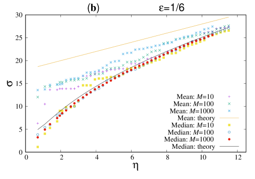
Figure 2: Plot of $\ln\bar{S}_{N}$ and $\ln\langle S_{N}\rangle$, as a function of $\eta=\ln N$, for $\epsilon=1/4$ (a) and $\epsilon=1/6$ (b).

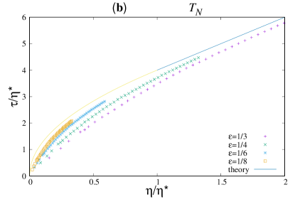
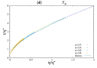
Figure 3: Plot of $\sigma/\eta^{\ast}$ (a) and $y^{\prime}=\tau/\tau^{\ast}$ (b) based upon median values, as a function of $\eta/\eta^{\ast}$, compared with the theoretical prediction for the $\epsilon\to 0$ limit, equation (63). In (c) and (d) we show similar plots for the upper octile data.

In figure 3, we plot $y=\sigma/\sigma^{\ast}$ (a) and $y^{\prime}=\tau/\tau^{\ast}$ (b) as a function of $x=\eta/\eta^{\ast}$, for all of the values of $\epsilon$ in our data set, using the largest sample size ($M=1000$) in each case, comparing with the theoretical scaling function (63). We see convergence towards the function (63) as $\epsilon\to 0$. In panels (c) and (d), we make the same comparison using the upper octile rather than the median.

5.2 Continuous potentials

In the case of a continuous potential, we require the mean separation of maxima or minima, $\tilde{x}$, in order to make a comparison with theory. The density ${\cal D}$ of zeros of $V^{\prime}(x)$ may be determined by the approach developed by Kac Kac1943 and Rice Rice1945 . If ${\cal P}(V,V^{\prime},V^{\prime\prime})$ is the joint PDF of $V(x)$ and its first two derivatives, evaluated at the same point, we find that

$${\cal D}=\int_{-\infty}^{\infty}{\rm d}V\int_{-\infty}^{\infty}{\rm d}V^{\prime\prime}\ {\cal P}(V,0,V^{\prime\prime})|V^{\prime\prime}|\ .$$ (64)

By noting that the vector $(V,V^{\prime},V^{\prime\prime})$ has a multivariate Gaussian distribution, and expressing ${\cal P}(V,V^{\prime},V^{\prime\prime})$ in terms of the correlation function of the elements of this vector, we obtain ${\cal D}$ and hence the separation of minima $\tilde{x}$ for the potential satisfying (57):

$$\frac{2}{\tilde{x}}\equiv{\cal D}=\frac{\sqrt{3}}{2\pi}\ .$$ (65)

First we investigated whether the mean-first passage time can be accurately represented by sums over maxima and minima of the potential. In figure 4, we compare the numerical evaluation of the integrals $S(x)$ (a) and $T(x)$ (b), given by Eq. (16) and Eq. (19), respectively, with the approximations which estimate the integrals using maxima and minima, Eq. (20).

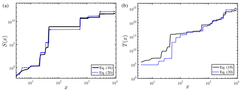
Figure 4: Plots of $S(x)$ (a) and $T(x)$ (b), for one realisation of the smooth random potential, with $D=1/8$. The numerically evaluated integrals (solid curves) are in good agreement with approximations based on sums over maxima and minima (dashed lines).

We evaluated the median $\bar{T}(x)$ and mean $\langle T(x)\rangle$ of the mean first passage time $T(x)$ for $1000$ realisations of the potential $V(x)$, up to $x_{\rm max}=10^{4}$, for $D\in\{1/3,1/4,1/5,1/6,1/7\}$. According to the discussion in section 4, we expect that $\tau=\ln\bar{T}(x)$ and $\eta=\ln(x/\tilde{x})$ are related by $\eta=J(D\tau/2)=D^{2}\tau^{2}/8$, up to a maximum value of $\eta$, given by $\eta^{\ast}=1/2D^{2}$. In figure 5 we plot $Y_{\rm med}=2D^{2}\ln\bar{T}(x)$ and $Y_{\rm av}=2D^{2}\ln\langle T(x)\rangle$ as a function of $X=2D^{2}\ln(x/\tilde{x})$ for different values of $D$, and compare with the theoretical scaling function, given by equation (63).

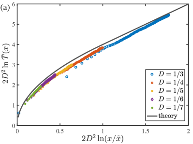
Figure 5: Numerical results on the median $\bar{T}(x)$ of the mean first-passage time to reach $x$, for different values of the diffusion coefficient $D$. We plot logarithmic variables $Y_{\rm med}=D^{2}\ln\bar{T}(x)/2$ (a) and $Y_{\rm av}=D^{2}\ln\langle T(x)\rangle$ (b) as a function of $X=2D^{2}\ln(x/\tilde{x})$ (where $\tilde{x}$ is the mean distance between maxima of $V(x)$). The numerical results converge towards the theoretically predicted scaling function, equation (63), as $D\to 0$.

6 Conclusions

In his analysis of equation (1), Zwanzig considered the mean-first-passsage time $T(x)$ to reach displacement $x$. Computing the expectation value $\langle T(x)\rangle$ over different realisations of the random potential, he showed Zwanzig1988 that $\langle T(x)\rangle\sim x^{2}$, which is consistent with a diffusive dispersion, with an effective diffusion coefficient $D_{\rm eff}$. The effective diffusion coefficient vanishes in a highly singular manner as $D\to 0$, and numerical studies have suggested that equation (1) exhibits anomalous diffusion Khoury2011 ; Simon2013 ; Goychuk2017 . It seems evident that the discrepancy between these two pictures of the dynamics results from the expectation value $\langle T(x)\rangle$ being dominated by rare events, where an unusually large fluctuation of the potential $V(x)$ acts as a barrier to dispersion. The central limit theorem is applicable to this problem, and at sufficiently large values of $x$ the ratio $T(x)/\langle T(x)\rangle$ is expected to approach unity, for almost all realisations of $V(x)$. However, at values of $x$ which are of practical relevance, most realisations $T(x)$ will be much smaller than $\langle T(x)\rangle$.

In order to give a description of the dynamics of (1) which is both empirically useable and analytically tractable, we considered the median (with respect to different realisations of the potential) of the mean-first-passage time. In the limit where the diffusion coefficient $D$ is small, the integrals which appear in the expression for the first passage time, equation (9), are dominated by maxima and minima of the potential, described by equations (17) and (20). This observation led us to consider the statistics of sums of exponentials of random variables, equations (8) and (21). We gave a quite precise estimate, equation (41), for the median of (8) and also derived simple relations describing the asymptotic behaviour of these sums, equations (47) and (49).

It is these expressions which enable us to formulate a concise asymptotic description of the dynamics of (1) in the limit as $D\to 0$, in terms of the large deviation rate function of the potential, $J(V)$. We argued that at very long length scales $\bar{T}(x)$ approaches the expectation value $\langle T(x)\rangle$, and that the dispersion is diffusive, in accord with the theory of Zwanzig Zwanzig1988 . On shorter timescales $\bar{T}(x)$ is determined by a ‘flooding’ model, according to which the probability density for locating the particle occupies a region which is constrained by a potential barrier which can trap a particle for time $\bar{T}$. As $\bar{T}$ increases, higher and higher barriers are required. For a Gaussian distribution of barrier heights, equation (4) implies that the dispersion is described as sub-diffusive, of the form

$$x\sim\tilde{x}\exp\left(\frac{D^{2}(\ln\bar{T})^{2}}{8C(0)}\right)$$ (66)

which is distinctively different from the power-law anomalous diffusion which has been reported by some authors Khoury2011 ; Simon2013 ; Goychuk2017 . Our numerical investigations of the dynamics of equation (1) for different values of $D$, illustrated in figure 5, show a data collapse which is in excellent agreement with equation (63), verifying (66).

Acknowledgments. We thank Baruch Meerson for bringing Zwanzig1988 to our notice, and for interesting discussion about the statistics of barrier heights. MW thanks the Chan-Zuckerberg Biohub for their hospitality.

References

- (1) Havlin, S. and Ben-Avraham, D., Diffusion in disordered media Advances in Physics, 51(1) 187–292, (2002).
- (2) Chaikin, P., and Lubensky, T., Principles of Condensed Matter Physics, Cambridge: University Press, (1995).
- (3) Saxton, M. J., A Biological Interpretation of Transient Anomalous Subdiffusion. I. Qualitative Model Biophysical Journal, 92(4) 1178-1191, (2007).
- (4) Zwanzig, R., 1988, Diffusion in a rough potential, PNAS, 85, 2029-30.
- (5) De Gennes, P. G., 1975, Brownian motion of a classical particle through potential barriers. Application to the helix-coil transitions of heteropolymers, J. Stat. Phys., 12, 463?81.
- (6) Khoury, M., Lacasta, A.M., Sancho, J.M. and Lindenberg, K., Weak Disorder: Anomalous transport and diffusion are normal yet again, Physical Review Letters, 106, 090602, (2011).
- (7) Simon, M. S., Sancho, J. M. and Lindenberg, K., Transport and diffusion of overdamped Brownian particles in random potentials, Physical Review E, 88, 062105, (2013).
- (8) Goychuk, I., Kharchenko, V. O. and Metzler, R., 2017, Persistent Sinai-type diffusion in Gaussian random potentials with decaying spatial correlations, Phys. Rev. E, 96, 052134.
- (9) Sinai, G. Ya., 1982, Theor. Prob. Appl., 27, 256.
- (10) Comtet, A. and Dean, D. S., 1998, Exact results on Sinai’s diffusion, J. Phys. A: Math. Gen., 31, 8595-8605.
- (11) Le Doussal, P., Monthus, C. and Fisher, D. S., 1999, Random walkers in one-dimensional random environments: Exact renormalization group analysis, Phys. Rev. E, 5, 4795-4840.
- (12) Kramers, H. A., Brownian motion in a field of force and the diffusion model of chemical reactions, Physica, 7, 284-304, (1940).
- (13) Redner, S., 2001, A guide to first-passage processes, Cambridge, University press, ISBN 0-521-65248-0.
- (14) Lifson, S. and Jackson, J. L., 1962, On self-diffusion of ions in a polyelectrolyte solution, J. Chem. Phys., 36, 2410-14.
- (15) M. Romeo, V. Da Costa, and F. Bardou, Broad distribution effects in sums of lognormal random variables, Eur. Phys. J. B, 32, 513-525, (2003).
- (16) M. Pradas, A. Pumir, and M. Wilkinson, Uniformity transition for ray intensities in random media, J. Phys. A: Math. Teor., 51, 155002, (2018).
- (17) Kac, M, 1943, On the average number of real roots of a random algebraic equation, Bull. Am. Math. Soc., 49, 314-20.
- (18) Rice, S O, 1945, Mathematical analysis of random noise, Bell Syst. Tech. J., 23, 283-332.