Spectral properties of local gauge invariant composite operators in the $SU(2)$ Yang–Mills–Higgs model

Abstract

The spectral properties of a set of local gauge (BRST) invariant composite operators are investigated in the $SU(2)$ Yang–Mills–Higgs model with a single Higgs field in the fundamental representation, quantized in the ’t Hooft $R_{\xi}$-gauge. These operators can be thought of as a BRST invariant version of the elementary fields of the theory, the Higgs and gauge fields, with which they share a gauge independent pole mass. The two-point correlation functions of both BRST invariant composite operators and elementary fields, as well as their spectral functions, are investigated at one-loop order. It is shown that the spectral functions of the elementary fields suffer from a strong unphysical dependence from the gauge parameter $\xi$, and can even exhibit positivity violating behaviour. In contrast, the BRST invariant local operators exhibit a well defined positive spectral density.

I Introduction

The principle of gauge invariance is the ultimate guideline to formulate quantum field theories of the fundamental interactions as, for example, the electroweak theory ’t Hooft et al. (1980); Peskin and Schroeder (1995). In non-Abelian gauge theories, genuine local gauge invariant quantities are associated to composite operators. It is therefore remarkable that the Standard Model is successfully described by employing non-gauge invariant fields as the Higgs and the $W$ and $Z$ elementary fields. Needless to say, the high order calculations of the pole masses and cross sections worked out by means of these non-gauge invariant fields are in very accurate agreement with the experimental data, see e.g. Jegerlehner et al. (2002, 2003); Martin (2015a, b) for a few illustrations.

At the theoretical level, the gauge parameter independence of the pole masses of both transverse $W$ and $Z$ bosons as well as of the Higgs field two-point correlation functions are understood by means of the so-called Nielsen identities Nielsen (1975); Aitchison and Fraser (1984); Piguet and Sibold (1985); Gambino et al. (1999); Gambino and Grassi (2000); Grassi et al. (2001); Andreassen et al. (2015), which follow from the Slavnov-Taylor identities encoding the exact BRST symmetry of quantized non-Abelian gauge theories. Nevertheless, as one easily figures out, the direct use of the non-gauge invariant fields displays several limitations, which become more severe in the case of a non-Abelian gauge theory. For instance, in the case of the $U(1)$ Higgs model, the transverse component of the Abelian gauge field $A_{\mu}$ is gauge invariant, so that the two-point correlation function $\mathcal{P}_{\mu\nu}(p)\langle A_{\mu}(p)A_{\nu}(-p)\rangle$, where $\mathcal{P}_{\mu\nu}(p)=(\delta_{\mu\nu}-\frac{p_{\mu}p_{\nu}}{p^{2}})$ is the transverse projector, turns out to be independent from the gauge parameter $\xi$. However, this is no more true in the non-Abelian case, where both Higgs and gauge boson two-point functions, i.e. $\langle h(p)h(-p)$ and $\mathcal{P}_{\mu\nu}(p)\langle A^{a}_{\mu}(p)A^{b}_{\nu}(-p)\rangle$, where $h$ stands for the Higgs field and $A^{a}_{\mu}$ for the gauge boson field, exhibit a strong gauge dependence from $\xi$. As a consequence, the understanding of the two-point correlation functions of both Higgs field $h$ and gauge vector boson $A^{a}_{\mu}$ in terms of the Källén-Lehmann (KL) spectral representation is completely jeopardized by an unphysical dependence from the gauge parameter $\xi$, obscuring a direct interpretation of the above mentioned correlation functions in terms of the elementary excitations of the physical spectrum, namely the Higgs and the vector gauge boson particles. We also note here that from a lattice perspective, it is expected that the spectrum of a gauge (Higgs) theory should be describable in terms of local gauge invariant operator correlation functions, with concrete physical information hiding in the various (positive and gauge invariant) spectral functions, not only pole masses, decay widths, but also transport coefficients at finite temperature etc. Clearly, such information will not correctly be encoded in gauge variant, non-positive spectral functions.

Within this perspective, the use of manifest gauge invariant variables to describe the Higgs and the vector gauge bosons is certainly very welcome. This endeavour was first proposed by ’t Hooft in ’t Hooft et al. (1980), and later on formalized by Fröhlich, Morchio and Strocchi (FMS) in Frohlich et al. (1980, 1981). These authors were able to build, out of the elementary fields, a set of local composite gauge invariant operators $\{\tilde{\mathcal{O}}(x)\}$ which, when expanded around the value $\Phi=constant$ which minimizes the Higgs potential present in the starting classical action, give rise to two-point functions which enjoy the important property of reproducing, at the tree level, the two-point correlation functions of the elementary fields $\{\varphi\}=(A^{a}_{\mu},h)$, namely

$$\braket{\tilde{\mathcal{O}}(x)\tilde{\mathcal{O}}(y)}\sim\braket{\varphi(x)\varphi(y)}_{\rm tree}+\ldots,$$ (1)

where $\ldots$ denote the higher order loop corrections which will be the main subject of the present work. Equation (1) shows in a very simple and intuitive way the relevance of the composite operators $\{\tilde{\mathcal{O}}(x)\}$ in order to provide a description of the gauge vector bosons and of the Higgs particle within a fully gauge invariant environment, see also the recent works Maas (2015, 2019); Maas and Törek (2018); Sondenheimer (2020) where, amongst other things, a lattice formulation has been proposed. Certain aspects of a gauge invariant version of the Higgs phenomenon were also covered in Kondo (2016, 2018), albeit whilst assuming the “frozen” radial limit, $\varphi^{\dagger}\varphi=\textrm{fixed}$, corresponding to a Higgs coupling $\lambda\to\infty$, a formal limit hampering explicit computations in the continuum.

In two earlier works Dudal et al. (2019, 2020a), we have laid the ground for the study of the spectral properties of the gauge (BRST) invariant local composite operators $\{\tilde{\mathcal{O}}(x)\}$ in the FMS framework. In Dudal et al. (2020a), we have made the first analytic one-loop calculations of these BRST invariant operators in the simpler $U(1)$ Higgs model quantized in the $R_{\xi}$-gauge. In particular, we have worked out the one-loop corrections to the two-point functions in eq. (1) corresponding to the Higgs and Abelian gauge fields and we have shown that they have the same gauge independent pole masses of the corresponding elementary two-point correlation functions. In addition, we have explicitly shown that the correlation functions of the composite operators display a well defined positive and gauge independent Källén-Lehmann spectral representation, a feature not shared by the two-point correlation functions of the elementary fields which, as in the explicit case of the Higgs field, i.e. $\langle h(p)h(-p)\rangle$, display an unphysical dependence from the gauge parameter $\xi$, becoming even negative depending on the value of $\xi$. Moreover, in Capri et al. (2020), the renormalization properties of these composite operators were scrutinized using the algebraic renormalization approach.

The aim of the present work is that of extending the techniques of Dudal et al. (2019, 2020a) to the more complex case of $SU(2)$ Higgs model with a single Higgs field in the fundamental representation. As we shall see, besides the exact BRST invariance, the quantized theory exhibits a global $SU(2)$ symmetry commonly referred to as the custodial symmetry. Moreover, the local composite BRST invariant operators corresponding to the gauge bosons transform as a triplet under the custodial symmetry, a property which will imply useful relations for their two-point correlation functions.

The present work is organized as follows. In section II, we give a review of the $SU(2)$ Yang–Mills–Higgs model with a single Higgs field in the fundamental representation, of the gauge fixing procedure and its ensuing BRST invariance. In section III we calculate the two-point correlation functions of the elementary fields up to one-loop order. In section IV, we define the BRST invariant local composite operators $(O(x),R^{a}_{\mu}(x))$ corresponding to the BRST invariant extension of $(h,A^{a}_{\mu})$ and calculate their one-loop correlation functions. In section V, we discuss the spectral properties of both elementary and composite operators.

In order to give a more general idea of the behavior of the spectral functions, we shall be using two sets of parameters which we shall refer as to Region I and Region II. To some extent, Region II can be associated to the perturbative weak coupling regime, while in Region I we keep the gauge coupling a little bit larger, while decreasing the vev (vacuum expectation value) of the Higgs field. Section VI is devoted to our conclusion and outlook. The technical details are all collected in the Appendices.

II The action and its symmetries

The Yang–Mills action with a single Higgs field in the fundamental representation is given by

$$S_{0} = \int d^{4}x\left\{\frac{1}{4}F_{\mu\nu}^{a}F_{\mu\nu}^{a}+(D_{\mu}^{ij}\Phi^{\dagger j})(D_{\mu}^{ik}\Phi^{k})+\frac{\lambda}{2}(\Phi^{\dagger i}\Phi^{i}-\frac{1}{2}v^{2})^{2}\right\}$$ (2)

$$= S_{\rm YM}+S_{\rm Higgs}$$

with

$$F_{\mu\nu}=\partial_{\mu}A_{\nu}^{a}-\partial_{\nu}A_{\mu}^{a}+g\epsilon^{abc}A_{\mu}^{b}A_{\nu}^{c}$$ (3)

and

$$D_{\mu}^{ij}\Phi^{j}=\partial_{\mu}\Phi^{i}-\frac{i}{2}g(\tau^{a})^{ij}A_{\mu}^{a}\Phi^{j},\,\,\,(D_{\mu}^{ij}\Phi^{j})^{\dagger}=\partial_{\mu}\Phi^{i\dagger}+\frac{i}{2}g\Phi^{j\dagger}(\tau^{a})^{ji}A_{\mu}^{a},$$ (4)

with the Pauli matrices $\tau^{a}(a=1,2,3)$ and the Levi-Civita tensor $\epsilon^{abc}$ referring to the gauge symmetry group $SU(2)$. The scalar complex field $\Phi^{i}(x)$ is in the fundamental representation of $SU(2)$, i.e. $i,j=1,2$. Thus, $\Phi$ is an $SU(2)$-doublet of complex scalar fields that can be written as

$$\Phi = \frac{1}{\sqrt{2}}\begin{pmatrix}\phi^{+}\\ \phi^{0}\end{pmatrix}=\frac{1}{\sqrt{2}}\begin{pmatrix}\phi_{1}+i\phi_{2}\\ \phi_{3}+i\phi_{4}\end{pmatrix}.$$ (5)

The configuration which minimizes the Higgs potential in the expression (2) is

$$\braket{\Phi} =\frac{1}{\sqrt{2}}\begin{pmatrix}v\\ 0\end{pmatrix}$$ (6)

and we write down $\Phi(x)$ as an expansion around the configuration (6), so that

$$\Phi=\frac{1}{\sqrt{2}}\begin{pmatrix}v+h+i\rho_{3}\\ i\rho_{1}-\rho_{2}\end{pmatrix},$$ (7)

where $h$ is the Higgs field and $\rho^{a}$, $a=1,2,3$, the would-be Goldstone bosons. We can use the matrix notation:

$$\Phi=\frac{1}{\sqrt{2}}((v+h)\textbf{1}+i\rho^{a}\tau^{a})\cdot\begin{pmatrix}1\\ 0\end{pmatrix},$$ (8)

so that the second term in eq. (2) becomes

$$(D^{ij}_{\mu}\Phi^{j})^{\dagger}D_{\mu}^{ik}\Phi^{k} = \frac{1}{2}(1,0)\cdot\Bigg{[}\partial_{\mu}h\cdot\textbf{1}-i\partial_{\mu}\rho^{a}\tau^{a}+\frac{ig}{2}\tau^{a}A_{\mu}^{a}\Big{(}(v+h)\textbf{1}-i\rho^{b}\tau^{b}\Big{)}\Bigg{]}$$

$$\times \Bigg{[}\partial_{\mu}h\cdot\textbf{1}+i\partial_{\mu}\rho^{c}\tau^{c}-\frac{ig}{2}((v+h)\textbf{1}-i\rho^{d}\tau^{d}\Big{)}\tau^{c}A_{\mu}^{c}\Bigg{]}\cdot\begin{pmatrix}1\\ 0\end{pmatrix}$$

$$= \tilde{\mathcal{L}_{0}}+\tilde{\mathcal{L}_{1}}+\tilde{\mathcal{L}_{2}},$$ (10)

with $\tilde{\mathcal{L}_{i}}$ the $i$th term in powers of $A_{\mu}$:

$$\tilde{\mathcal{L}}_{0} = \frac{1}{2}\left((\partial_{\mu}h)^{2}+\partial_{\mu}\rho^{a}\partial_{\mu}\rho^{a}\right),$$

$$\tilde{\mathcal{L}}_{1} = -\frac{1}{2}\left\{gvA_{\mu}^{a}\partial_{\mu}\rho^{a}-gA_{\mu}^{a}\rho^{a}\partial_{\mu}h+gA_{\mu}^{a}(\partial_{\mu}\rho^{a})h+g\epsilon^{abc}\partial_{\mu}\rho^{a}\rho^{b}A_{\mu}^{c}\right\},$$

$$\tilde{\mathcal{L}_{2}} = \frac{g^{2}}{8}A_{\mu}^{a}A_{\mu}^{a}\left[(v+h)^{2}+\rho^{b}\rho^{b}\right],$$ (11)

and we have the full action

$$S_{0} = \int d^{4}x\frac{1}{2}\Bigg{\{}\frac{1}{2}F^{a}_{\mu\nu}F^{a}_{\mu\nu}+\frac{1}{4}v^{2}g^{2}A_{\mu}^{a}A_{\mu}^{a}+(\partial_{\mu}h)^{2}+\partial_{\mu}\rho^{a}\partial_{\mu}\rho^{a}-gvA_{\mu}^{a}\partial_{\mu}\rho^{a}+gA_{\mu}^{a}\rho^{a}\partial_{\mu}h-gA^{a}_{\mu}(\partial_{\mu}\rho^{a})h$$ (12)

$$- g\epsilon^{abc}\partial_{\mu}\rho^{a}\rho^{b}A_{\mu}^{c}+\frac{g^{2}}{4}A_{\mu}^{a}A_{\mu}^{a}\left[2vh+h^{2}+\rho^{b}\rho^{b}\right]+\lambda v^{2}h^{2}+\lambda vh(h^{2}+\rho^{a}\rho^{a})$$

$$+ \frac{\lambda}{4}(h^{2}+\rho^{a}\rho^{a})^{2}\Bigg{\}}.$$

One sees that both gauge field $A^{a}_{\mu}$ and Higgs field $h$ have acquired a mass given, respectively, by

$$m^{2}=\frac{1}{4}g^{2}v^{2},\,\,\,\,\,\,\,m_{h}^{2}=\lambda v^{2}\;.$$ (13)

II.1 Gauge fixing and BRST symmetry

The action (2) is invariant under the local $\omega$-parametrized gauge transformations

$$\delta A_{\mu}^{a}=-D_{\mu}^{ab}\omega^{b},\,\,\,\delta\Phi=-\frac{ig}{2}\omega^{a}\tau^{a}\Phi,\,\,\,\delta\Phi^{\dagger}=\frac{ig}{2}\omega^{a}\Phi^{\dagger}\tau^{a},$$ (14)

which, when written in terms of the fields $(h,\rho^{a})$, become

$$\delta h=\frac{g}{2}\omega^{a}\rho^{a},\,\,\,\delta\rho^{a}=-\frac{g}{2}(\omega^{a}(v+h)\textbf{1}-\epsilon^{abc}\omega^{b}\rho^{c}).$$ (15)

As done in the $U(1)$ case Dudal et al. (2019, 2020a), we shall be using the $R_{\xi}$-gauge. We add thus need the gauge fixing term

$$\mathcal{S}_{\rm gf} = s\int d^{4}x\Bigl{\{}-i\frac{\xi}{2}\bar{c}^{a}b^{a}+\bar{c}^{a}(\partial_{\mu}A_{\mu}^{a}-\xi m\rho^{a})\Bigr{\}}$$ (16)

$$= \frac{1}{2}\int d^{4}x\Bigl{\{}\xi b^{a}b^{a}+2ib^{a}\partial_{\mu}A_{\mu}^{a}+2\bar{c}^{a}\partial_{\mu}D_{\mu}^{ab}c^{b}-2i\xi mb^{a}\rho^{a}$$

$$- 2\xi\bar{c}^{a}mc^{a}-g\xi\bar{c}^{a}mhc^{a}-\xi g\epsilon^{abc}\bar{c}^{a}c^{b}\rho^{c}\Bigr{\}}\;,$$

so that the gauge fixed action $S_{\text{full}}=S_{0}+\mathcal{S}_{\rm gf}$, namely

$$S_{\text{full}} = \int d^{4}x\frac{1}{2}\Bigg{\{}\frac{1}{2}F^{a}_{\mu\nu}F^{a}_{\mu\nu}+\frac{1}{4}v^{2}g^{2}A_{\mu}^{a}A_{\mu}^{a}$$ (17)

$$+ (\partial_{\mu}h)^{2}+\partial_{\mu}\rho^{a}\partial_{\mu}\rho^{a}-gvA_{\mu}^{a}\partial_{\mu}\rho^{a}+gA_{\mu}^{a}\rho^{a}\partial_{\mu}h-gA^{a}_{\mu}(\partial_{\mu}\rho^{a})h$$

$$- g\epsilon^{abc}\partial_{\mu}\rho^{a}\rho^{b}A_{\mu}^{c}+\frac{g^{2}}{4}A_{\mu}^{a}A_{\mu}^{a}\left[2vh+h^{2}+\rho^{b}\rho^{b}\right]+\lambda v^{2}h^{2}$$

$$+ \lambda vh(h^{2}+\rho^{a}\rho^{a})+\frac{\lambda}{4}(h^{2}+\rho^{a}\rho^{a})^{2}+\xi b^{a}b^{a}+2ib^{a}\partial_{\mu}A_{\mu}^{a}+2\bar{c}^{a}\partial_{\mu}D_{\mu}^{ab}c^{b}-2i\xi mb^{a}\rho^{a}$$

$$- 2\xi\bar{c}^{a}mc^{a}-g\xi\bar{c}^{a}mhc^{a}-\xi g\epsilon^{abc}\bar{c}^{a}c^{b}\rho^{c}\Bigg{\}}$$

turns out to be left invariant by the BRST transformations

$$sA_{\mu}^{a} = -D_{\mu}^{ab}c^{b},\,\,\,sh=\frac{g}{2}c^{a}\rho^{a},\,\,\,s\rho^{a}=-\frac{g}{2}(c^{a}(v+h)-\epsilon^{abc}c^{b}\rho^{c})$$

$$sc^{a} = \frac{1}{2}g\epsilon^{abc}c^{b}c^{c},\,\,\,s\bar{c}^{a}=ib^{a},\,\,\,sb^{a}=0\;,$$ (18)

$$sS_{\text{full}}=0\;.$$ (19)

The Feynman rules for the full action (17) are given in Appendix A. Notice that in the $R_{\xi}$-gauge the tree-level propagator $\braket{A^{a}_{\mu}(x)\rho^{a}(y)}$ vanishes, a well-known feature of this gauge choice Peskin and Schroeder (1995). We will assume that $\xi\geq 0$ to avoid tachyon poles in elementary propagators, see eq. (A).

II.2 Custodial symmetry

As already mentioned, apart from the BRST symmetry, there is an extra global symmetry, which we shall refer to as the custodial symmetry:

$$\delta A^{a}_{\mu} = \epsilon^{abc}\beta^{b}A^{c}_{\mu},$$

$$\delta\rho^{a} = \epsilon^{abc}\beta^{b}\rho^{c},$$

$$\delta\overline{c}^{a} = \epsilon^{abc}\beta^{b}\overline{c}^{c},$$

$$\delta c^{a} = \epsilon^{abc}\beta^{b}c^{c},$$

$$\delta b^{a} = \epsilon^{abc}\beta^{b}b^{c},$$

$$\delta h = 0\;,$$ (20)

where $\beta^{a}$ is a constant parameter, $\partial_{\mu}\beta^{a}=0$,

$$\delta S_{\text{full}}=0\;.$$ (21)

One notices that all fields carrying the index $a=1,2,3$, i.e. $(A^{a}_{\mu},b^{a},c^{a},{\bar{c}}^{a},\rho^{a})$, undergo a global transformation in the adjoint representation of $SU(2)$. The origin of this symmetry is an $SU(2)_{\rm gauge}\times SU(2)_{\rm global}$ symmetry of the action in the unbroken phase, see Appendix B. The exception is the Higgs field $h$, which is left invariant, i.e. it is a singlet. As we shall see in the following, this additional global symmetry will provide useful relationships for the two-point correlation functions of the BRST invariant composite operators.

III One-loop evaluation of the correlation function of the elementary fields

For the elementary fields $h(x)$ and $A^{a}_{\mu}$, the correlation functions are calculated up to first loop order in Appendices C.0.1 and C.0.2. In what follows, we will always spell out again the momentum-dependent logarithms and explicit Feynman parameter dependence, that is, we will in the eventual correlation functions replace again the notational shorthands introduced in eq. (C). The Feynman parameter integration itself was handled via (147). We have used the explicit expression (147) to numerically construct our spectral function plots (see later). More about that integral (147) can be found in ’t Hooft and Veltman (1979); Ellis and Zanderighi (2008).

For the Higgs field, for the propagator we get

$$\braket{h(p)h(-p)} = \frac{1}{p^{2}+m_{h}^{2}}+\frac{1}{(p^{2}+m_{h}^{2})^{2}}\Pi_{hh}(p^{2})+\mathcal{O}(\hbar^{2}),$$ (22)

with $\Pi_{hh}(p^{2})$ the one-loop correction to the self-energy calculated in Appendix C.0.1. For $d=4$, this correction is divergent. Employing the procedure of dimensional regularization, i.e. setting $d=4-\epsilon$, the divergent part for $\Pi_{hh}(p^{2})$ is given by:

$$\Pi_{hh,\rm div}(p^{2}) = \frac{g^{2}\left(\frac{3m_{h}^{4}}{m^{2}}-3\xi m_{h}^{2}-3\xi p^{2}+9p^{2}\right)}{32\pi^{2}\epsilon},$$ (23)

which, following the $\overline{\mbox{MS}}$-scheme, is re-absorbed by the introduction of suitable local counterterms. We remain thus with the finite part of the Higgs self-energy

$$\Pi_{hh}(p^{2}) = \frac{3g^{2}}{{8(4\pi)^{2}}}\int_{0}^{1}dx\,\Bigg{\{}2\xi\left(m_{h}^{2}+p^{2}\right)\ln\left(\frac{m^{2}\xi}{\mu^{2}}\right)-2\xi m_{h}^{2}+2\left(6m^{2}-p^{2}\right)\ln\left(\frac{m^{2}}{\mu^{2}}\right)$$ (24)

$$- (12m^{2}+\frac{p^{4}}{m^{2}}+4p^{2})\ln\left(\frac{m^{2}+p^{2}(1-x)x}{\mu^{2}}\right)+\left(\frac{p^{4}}{m^{2}}-\frac{m_{h}^{4}}{m^{2}}\right)\ln\left(\frac{m^{2}\xi+p^{2}(1-x)x}{\mu^{2}}\right)-12m^{2}-2\xi p^{2}+2p^{2}$$

$$- \frac{m_{h}^{4}}{m^{2}}\left(-2\ln\left(\frac{m_{h}^{2}}{\mu^{2}}\right)+3\ln\left(\frac{m_{h}^{2}+p^{2}(1-x)x}{\mu^{2}}\right)+2\right)\Bigg{\}}.$$

Before trying to resum the self-energy $\Pi_{hh}(p^{2})$, we notice that this resummation is tacitly assuming that the second term in (22) is much smaller than the first term. However, we see that eq. (22) contains terms of the order of $\frac{p^{4}}{(p^{2}+m_{h}^{2})^{2}}\ln\left(\frac{m^{2}+p^{2}(1-x)x}{\mu^{2}}\right)$ which cannot be resummed for big values of $p^{2}$.

Indeed, if one proceeds naively and include these large contributions into a resummation, spurious tachyon poles will be induced in the correlator, analogous as in the earlier investigated $U(1)$ case in Dudal et al. (2020a). The need for care in resumming these contributions was also strengthened and worked out in great detail in Maas and Sondenheimer (2020).

We therefore proceed as in Dudal et al. (2019, 2020a) and use the identity

$$p^{4}=(p^{2}+m_{h}^{2})^{2}-m_{h}^{4}-2p^{2}m_{h}^{2}$$ (25)

to rewrite

$$\frac{p^{4}}{(p^{2}+m_{h}^{2})^{2}}\ln\frac{p^{2}x(1-x)+m^{2}}{\mu^{2}} = \ln\frac{p^{2}x(1-x)+m^{2}}{\mu^{2}}-\underline{\frac{(m_{h}^{4}+2p^{2}m_{h}^{2})}{(p^{2}+m_{h}^{2})^{2}}\ln\frac{p^{2}x(1-x)+m^{2}}{\mu^{2}}}.$$ (26)

The term which has been underlined in eq. (26) can be safely resummed, as it decays fast enough for large values of $p^{2}$. We thence rewrite

$$\frac{{\Pi}_{hh}(p^{2})}{(p^{2}+m_{h}^{2})^{2}} = \frac{\hat{\Pi}_{hh}(p^{2})}{(p^{2}+m_{h}^{2})^{2}}+C_{hh}(p^{2})\;,$$ (27)

with

$$\hat{\Pi}_{hh}(p^{2}) = \frac{3g^{2}}{{8(4\pi)^{2}}}\int_{0}^{1}dx\,\Bigg{\{}2\xi\left(m_{h}^{2}+p^{2}\right)\ln\left(\frac{m^{2}\xi}{\mu^{2}}\right)-2\xi m_{h}^{2}+2\left(6m^{2}-p^{2}\right)\ln\left(\frac{m^{2}}{\mu^{2}}\right)$$ (28)

$$- (12m^{2}-\frac{(m_{h}^{4}+2p^{2}m_{h}^{2})}{m^{2}}+4p^{2})\ln\left(\frac{m^{2}+p^{2}(1-x)x}{\mu^{2}}\right)-\frac{(2m_{h}^{4}+2p^{2}m_{h}^{2})}{m^{2}}\ln\left(\frac{m^{2}\xi+p^{2}(1-x)x}{\mu^{2}}\right)$$

$$- 12m^{2}-2\xi p^{2}+2p^{2}-\frac{m_{h}^{4}}{m^{2}}\Big{(}-2\ln\left(\frac{m_{h}^{2}}{\mu^{2}}\right)+3\ln\left(\frac{m_{h}^{2}+p^{2}(1-x)x}{\mu^{2}}\right)+2\Big{)}\Bigg{\}}$$

and

$$C_{hh}(p^{2})=-\frac{3g^{2}}{{8m^{2}(4\pi)^{2}}}\int_{0}^{1}dx\left(\ln\frac{p^{2}x(1-x)+m^{2}}{\mu^{2}}-\ln\frac{p^{2}x(1-x)+\xi m^{2}}{\mu^{2}}\right)\;.$$ (29)

Thus, for the one-loop Higgs propagator, we get

$$\braket{h(p)h(-p)} = \frac{1}{p^{2}+m_{h}^{2}-\hat{\Pi}_{hh}(p^{2})}+C_{hh}(p^{2})+\mathcal{O}(\hbar^{2})\;.$$ (30)

For the gauge field, we split the two-point function into transverse and longitudinal parts in the usual way

$$\braket{A_{\mu}^{a}(p)A^{b}_{\nu}(-p)}=\braket{A_{\mu}^{a}(p)A^{b}_{\nu}(-p)}^{T}\mathcal{P}_{\mu\nu}(p)+\braket{A_{\mu}^{a}(p)A^{b}_{\nu}(-p)}^{L}\mathcal{L}_{\mu\nu}(p),$$ (31)

where we have introduced the transverse and longitudinal projectors, given respectively by

$$\mathcal{P}_{\mu\nu}(p) = \delta_{\mu\nu}-\frac{p_{\mu}p_{\nu}}{p^{2}}\,,\qquad\mathcal{L}_{\mu\nu}(p)~{}=~{}\frac{p_{\mu}p_{\nu}}{p^{2}}\,.$$ (32)

We find

$$\braket{A_{\mu}^{a}(p)A_{\nu}^{b}(-p)}^{T}=\frac{\delta^{ab}}{p^{2}+m^{2}}+\frac{\delta^{ab}}{(p^{2}+m^{2})^{2}}\Pi_{AA^{T}}(p^{2})+\mathcal{O}(\hbar^{2}),$$ (33)

with $\Pi_{AA^{T}}(p^{2})$ the one-loop correction to the self-energy calculated in Appendix C.0.2. For $d=4-\epsilon$, following the procedure of dimensional regularization, we find that the divergent part for $\Pi_{AA^{T}}(p^{2})$ is given by:

$$\Pi_{AA^{T},\rm div}(p^{2}) = \frac{g^{2}}{\pi^{2}\epsilon}\left(-\frac{9m^{4}}{16m_{h}^{2}}-\frac{3m_{h}^{2}}{32}-\frac{m^{2}\xi}{8}-\frac{3m^{2}}{32}-\frac{\xi p^{2}}{8}+\frac{25p^{2}}{48}\right),$$ (34)

and these terms can be, following the $\overline{\mbox{MS}}$-scheme, absorbed by means of appropriate counterterms. We remain with the finite part of the self-energy

$$\Pi_{AA^{T}}(p^{2}) = -\frac{\delta^{ab}g^{2}}{36(4\pi)^{2}m^{4}p^{2}m_{h}^{2}}\int_{0}^{1}dx\Bigg{\{}-27m^{4}p^{2}m_{h}^{4}\ln\left(\frac{m_{h}^{2}}{\mu^{2}}\right)-27m^{6}\xi p^{2}m_{h}^{2}\ln\left(\frac{m^{2}\xi}{\mu^{2}}\right)$$ (35)

$$+ 3m^{4}m_{h}^{4}\left(m_{h}^{2}-m^{2}+2p^{2}\right)\ln\left(\frac{m_{h}^{2}}{\mu^{2}}\right)+27m^{4}p^{2}m_{h}^{2}\left(m_{h}^{2}+m^{2}\xi\right)$$

$$- 3m^{4}\xi m_{h}^{2}\left(2m^{4}(\xi-1)+m^{2}(4\xi+7)p^{2}+2(\xi+9)p^{4}\right)\ln\left(\frac{m^{2}\xi}{\mu^{2}}\right)$$

$$+ 3m^{4}\ln\left(\frac{m^{2}}{\mu^{2}}\right)\left(-m^{2}m_{h}^{4}+m_{h}^{2}\left(m^{4}(2\xi-1)+m^{2}(4\xi+45)p^{2}+2(\xi+9)p^{4}\right)-54m^{4}p^{2}\right)$$

$$+ m^{4}\left(6m^{2}m_{h}^{4}+m_{h}^{2}\left(3m^{4}(2(\xi-2)\xi+1)+3m^{2}(\xi-1)(4\xi-1)p^{2}+2(3\xi(\xi+4)-17)p^{4}\right)-3m_{h}^{6}+54m^{4}p^{2}\right)$$

$$- 3m_{h}^{2}\Big{[}m^{4}\left(2p^{2}\left(m_{h}^{2}-5m^{2}\right)+\left(m_{h}^{2}-m^{2}\right){}^{2}+p^{4}\right)\ln\left(\frac{p^{2}(1-x)x+m_{h}^{2}(1-x)+m^{2}x}{\mu^{2}}\right)$$

$$- 2\left(m^{2}+p^{2}\right)^{2}\left(m^{4}(\xi-1)^{2}+2m^{2}(\xi-5)p^{2}+p^{4}\right)\ln\left(\frac{p^{2}(1-x)x+\xi m^{2}(1-x)+m^{2}x}{\mu^{2}}\right)$$

$$+ p^{2}\left(p^{4}-m^{4}\right)\left(4m^{2}\xi+p^{2}\right)\ln\left(\frac{p^{2}(1-x)x+\xi m^{2}}{\mu^{2}}\right)$$

$$+ p^{2}\left(4m^{2}+p^{2}\right)\left(12m^{4}-20m^{2}p^{2}+p^{4}\right)\ln\left(\frac{p^{2}(1-x)x+m^{2}}{\mu^{2}}\right)\Big{]}\Bigg{\}}.$$

We see that (33) contains again terms of the order $\frac{p^{4}}{(p^{2}+m^{2})^{2}}\ln\left(\frac{m^{2}+p^{2}(1-x)x}{\mu^{2}}\right)$ and $\frac{p^{6}}{(p^{2}+m^{2})^{2}}\ln\left(\frac{m^{2}+p^{2}(1-x)x}{\mu^{2}}\right)$, which cannot be resummed for big values of $p^{2}$. We use

$$\frac{p^{4}}{(p^{2}+m^{2})^{2}}\ln\frac{p^{2}x(1-x)+m^{2}}{\mu^{2}} = \ln\frac{p^{2}x(1-x)+m^{2}}{\mu^{2}}-\underline{\frac{(m^{4}+2p^{2}m^{2})}{(p^{2}+m^{2})^{2}}\ln\frac{p^{2}x(1-x)+m^{2}}{\mu^{2}}}$$ (36)

and

$$\frac{p^{6}}{(p^{2}+m^{2})^{2}}\ln\frac{p^{2}x(1-x)+m^{2}}{\mu^{2}} = (p^{2}-2m^{2})\ln\frac{p^{2}x(1-x)+m^{2}}{\mu^{2}}+\underline{\frac{2m^{6}+3p^{2}m^{4}}{(p^{2}+m^{2})^{2}}\ln\frac{p^{2}x(1-x)+m^{2}}{\mu^{2}}}.$$ (37)

The underlined terms in (36) and (37) can be safely resummed. We rewrite

$$\frac{{\Pi}_{AA^{T}}(p^{2})}{(p^{2}+m^{2})^{2}} = \frac{\hat{\Pi}_{AA^{T}}(p^{2})}{(p^{2}+m_{h}^{2})^{2}}+C_{AA^{T}}(p^{2}),$$ (38)

with

$$\hat{\Pi}_{AA^{T}}(p^{2}) = -\frac{\delta^{ab}g^{2}}{36(4\pi)^{2}m^{4}p^{2}m_{h}^{2}}\int_{0}^{1}dx\Bigg{\{}-27m^{4}p^{2}m_{h}^{4}\ln\left(\frac{m_{h}^{2}}{\mu^{2}}\right)-27m^{6}\xi p^{2}m_{h}^{2}\ln\left(\frac{m^{2}\xi}{\mu^{2}}\right)$$ (39)

$$+ 3m^{4}m_{h}^{4}\left(m_{h}^{2}-m^{2}+2p^{2}\right)\ln\left(\frac{m_{h}^{2}}{\mu^{2}}\right)+27m^{4}p^{2}m_{h}^{2}\left(m_{h}^{2}+m^{2}\xi\right)$$

$$- 3m^{4}\xi m_{h}^{2}\left(2m^{4}(\xi-1)+m^{2}(4\xi+7)p^{2}+2(\xi+9)p^{4}\right)\ln\left(\frac{m^{2}\xi}{\mu^{2}}\right)$$

$$+ 3m^{4}\left(-m^{2}m_{h}^{4}+m_{h}^{2}\left(m^{4}(2\xi-1)+m^{2}(4\xi+45)p^{2}+2(\xi+9)p^{4}\right)-54m^{4}p^{2}\right)\ln\left(\frac{m^{2}}{\mu^{2}}\right)$$

$$+ m^{4}\left(6m^{2}m_{h}^{4}+m_{h}^{2}\left(3m^{4}(2(\xi-2)\xi+1)+3m^{2}(\xi-1)(4\xi-1)p^{2}+2(3\xi(\xi+4)-17)p^{4}\right)-3m_{h}^{6}+54m^{4}p^{2}\right)$$

$$- 3m_{h}^{2}\Big{[}m^{4}\left(2p^{2}\left(m_{h}^{2}-5m^{2}\right)+\left(m_{h}^{2}-m^{2}\right){}^{2}+p^{4}\right)\ln\left(\frac{p^{2}(1-x)x+(1-x)m_{h}^{2}+m^{2}x}{\mu^{2}}\right)$$

$$- 2m^{4}(\xi-1)^{2}\left(m^{2}+p^{2}\right)^{2}\ln\left(\frac{p^{2}(1-x)x+\xi m^{2}(1-x)+m^{2}x}{\mu^{2}}\right)$$

$$+ \left(-2m^{4}(4\xi-1)p^{2}\left(m^{2}+p^{2}\right)\right)\ln\left(\frac{p^{2}(1-x)x+\xi m^{2}}{\mu^{2}}\right)$$

$$+ (66m^{6}p^{2}-33m^{4}p^{4})\ln\left(\frac{p^{2}(1-x)x+m^{2}}{\mu^{2}}\right)\Big{]}\Bigg{\}}.$$

and

$$C_{AA^{T}}(p^{2}) = \frac{\delta^{ab}g^{2}}{12(4\pi)^{2}m^{4}}\int_{0}^{1}dx\Bigg{\{}(-4m^{2}(\xi-5)-2p^{2})$$ (40)

$$\times \ln\left(\frac{p^{2}(1-x)x+\xi m^{2}(1-x)+m^{2}x}{\mu^{2}}\right)$$

$$+ \left(4\,\xi m^{2}+p^{2}-2m^{2}\right)\ln\left(\frac{p^{2}(1-x)x+\xi m^{2}}{\mu^{2}}\right)$$

$$+ (-18m^{2}+p^{2})\ln\left(\frac{p^{2}(1-x)x+m^{2}}{\mu^{2}}\right)\Bigg{\}}.$$

Finally

$$\braket{A_{\mu}^{a}(p)A_{\nu}^{b}(-p)}^{T}=\delta^{ab}\left(\frac{1}{p^{2}+m^{2}-\hat{\Pi}_{AA^{T}}(p^{2})}+C_{AA^{T}}(p^{2})\right)+\mathcal{O}(\hbar^{2})\;.$$ (41)

IV One-loop evaluation of the correlation function of the local BRST invariant composite operators

IV.1 Correlation function of the scalar BRST invariant composite operator $O(x)$

The gauge and BRST invariant local scalar composite operator $O(x)$ is given by

$$O(x)=\Phi^{\dagger}\Phi-\frac{v^{2}}{2}\;,\qquad s\;O(x)=0\;,$$ (42)

which, after using the expansion (8), becomes

$$O(x) = \frac{1}{2}\Big{[}\begin{pmatrix}1&0\end{pmatrix}((v+h)\textbf{1}-i\rho^{a}\tau^{a}))((v+h)\textbf{1}+i\rho^{b}\tau^{b}))\begin{pmatrix}1\\ 0\end{pmatrix}\Big{]}-\frac{v^{2}}{2}$$ (43)

$$= \frac{1}{2}\Big{(}h^{2}(x)+2vh(x)+\rho^{a}(x)\rho^{a}(x)\Big{)}\;.$$

Notice that the operator $O(x)$ does not depend on the FP ghost field. Therefore,

$$\braket{{O}(x){O}(y)} = v^{2}\braket{h(x)h(y)}+v\braket{h(x)\rho^{b}(y)\rho^{b}(y)}+v\braket{h(x)h(y)^{2}}+\frac{1}{4}\braket{h(x)^{2}\rho^{b}(y)\rho^{b}(y)}+\frac{1}{4}\braket{h(x)^{2}h(y)^{2}}$$ (44)

$$+ \frac{1}{4}\braket{\rho^{a}(x)\rho^{a}(x)\rho^{b}(y)\rho^{b}(y)}.$$

Looking at the tree level expression of eq. (44), one easily obtains

$$\braket{{O}(p){O}(-p)}_{\rm tree}=v^{2}\braket{h(p)h(-p)}_{\rm tree}=v^{2}\frac{1}{p^{2}+m_{h}^{2}}\;,$$ (45)

showing that the BRST invariant scalar operator $O(x)$ is directly linked to the Higgs propagator.

Concerning now the one-loop calculation of expression (44), after evaluating each term, see Appendix D for details, we find that the two-point correlation function of the scalar composite operator $O(x)$ develops a geometric series in the same way as the elementary field $h(x)$. This allows us the make a resummed approximation. Using dimensional regularization in the $\overline{\mbox{MS}}$-scheme, we find that, in the $R_{\xi}$-gauge

$$\braket{O(p)O(-p)}(p^{2}) = \frac{v^{2}}{p^{2}+m_{h}^{2}}+\frac{v^{2}\,}{(p^{2}+m_{h}^{2})^{2}}\Pi_{OO}(p^{2})+\mathcal{O}(\hbar^{2}),$$ (46)

with $\Pi_{OO}(p^{2})$ the one-loop correction calculated in Appendix D. Following the procedure of dimensional regularization for $d=4-\epsilon$, we find that the divergent part of the one-loop correction is given by

$$\Pi_{OO,\rm div}^{-1} = \frac{1}{4v^{2}\pi^{2}\epsilon}\Big{(}\frac{9g^{4}p^{2}v^{2}}{16\lambda}+\frac{9g^{4}v^{4}}{16}+\frac{9}{8}g^{2}p^{2}v^{2}+p^{4}+\frac{1}{2}\lambda p^{2}v^{2}+\lambda^{2}v^{4}\Big{)},$$ (47)

which can be accounted for by appropriate counterterms, following the $\overline{\mbox{MS}}$-scheme renormalization procedure. A full renormalization analysis will be presented elsewhere. Notice that expression (47), when multiplied again with the factored-out $v^{2}$ of eq. (46), is a polynomial in $p^{2},v^{2}$, in full accordance with power counting renormalizability.
We remain with the finite part, given by

$$\Pi_{OO}(p^{2}) = \frac{1}{{32v^{2}\pi^{2}m_{h}^{2}}}\int_{0}^{1}dx\Bigg{\{}-24m_{h}^{2}m^{4}-6m^{2}p^{2}\left(m_{h}^{2}+6m^{2}\right)\ln\left(\frac{m^{2}}{\mu^{2}}\right)$$ (48)

$$- m_{h}^{2}\left(p^{2}-2m_{h}^{2}\right)^{2}\ln\left(\frac{m_{h}^{2}+p^{2}x(1-x)}{\mu^{2}}\right)$$

$$- 3m_{h}^{2}\left(12m^{4}+4m^{2}p^{2}+p^{4}\right)\ln\left(\frac{m^{2}+p^{2}x(1-x)}{\mu^{2}}\right)$$

$$+ 6p^{2}\left(m_{h}^{4}+m_{h}^{2}m^{2}+2m^{4}\right)-6m_{h}^{4}p^{2}\ln\left(\frac{m_{h}^{2}}{\mu^{2}}\right)\Bigg{\}}.$$

Since (46) contains terms of the order of $\frac{p^{4}}{(p^{2}+m^{2})^{2}}\ln(p^{2})$, we follow the steps (36)-(38) to find the resummed correlation function in the one-loop approximation

$$G_{{O}{O}}(p^{2}) = \frac{v^{2}}{p^{2}+m_{h}^{2}-\hat{\Pi}_{OO}(p^{2})}+C_{OO}(p^{2})$$ (49)

with

$$\hat{\Pi}_{OO}(p^{2}) = \frac{1}{{32v^{2}\pi^{2}m_{h}^{2}}}\int_{0}^{1}dx\Bigg{\{}-24m_{h}^{2}m^{4}-6m^{2}p^{2}\left(m_{h}^{2}+6m^{2}\right)\ln\left(\frac{m^{2}}{\mu^{2}}\right)$$ (50)

$$- m_{h}^{2}(3m_{h}^{4}-6m_{h}^{2}p^{2})\ln\left(\frac{m_{h}^{2}+p^{2}x(1-x)}{\mu^{2}}\right)$$

$$- 3m_{h}^{2}\left(12m^{4}+4m^{2}p^{2}-m_{h}^{4}-2p^{2}m_{h}^{2}\right)\ln\left(\frac{m^{2}+p^{2}x(1-x)}{\mu^{2}}\right)$$

$$+ 6p^{2}\left(m_{h}^{4}+m_{h}^{2}m^{2}+2m^{4}\right)-6m_{h}^{4}p^{2}\ln\left(\frac{m_{h}^{2}}{\mu^{2}}\right)\Bigg{\}}$$

and

$$C_{OO}(p^{2}) = -\frac{1}{32\pi^{2}}\int_{0}^{1}dx\Bigg{\{}\ln\left(\frac{m_{h}^{2}+p^{2}x(1-x)}{\mu^{2}}\right)+3\ln\left(\frac{m^{2}+p^{2}x(1-x)}{\mu^{2}}\right)\Bigg{\}}.$$ (51)

Expressions (49) and (51) show that, as expected, and unlike the Higgs propagator, eq. (30), the correlator $\braket{O(p)O(-p)}$ is independent from the gauge parameter $\xi$.

IV.2 Vectorial composite operators

We identify three gauge invariant vector composite operators, following the definitions of ’t Hooft in ’t Hooft et al. (1980), namely

$$O_{\mu}^{3} = i\phi^{\dagger}D_{\mu}\phi,$$

$$O_{\mu}^{+} = \phi^{T}\begin{pmatrix}0&1\\ -1&0\end{pmatrix}D_{\mu}\phi,$$

$$O_{\mu}^{-} = (O_{\mu}^{+})^{\dagger}.$$ (52)

The gauge invariance of $O_{\mu}^{3}$ is apparent. For $O^{+}_{\mu}$, we can show the gauge invariance by using the following $2\times 2$ matrix representation of a generic $SU(2)$ transformation,

$$U=\begin{pmatrix}a&-b^{\star}\\ b&a^{\star}\end{pmatrix}$$ (53)

with determinant $|a|^{2}+|b|^{2}=1$. Thus, we find that under a $SU(2)$ transformation

$$O_{\mu}^{+} \rightarrow (U\phi)^{T}\begin{pmatrix}0&1\\ -1&0\end{pmatrix}D_{\mu}(U\phi)$$ (54)

$$= \phi^{T}U^{T}\begin{pmatrix}0&1\\ -1&0\end{pmatrix}UD_{\mu}\phi$$

$$= \phi^{T}\begin{pmatrix}0&1\\ -1&0\end{pmatrix}D_{\mu}\phi=O_{\mu}^{+},$$

which shows the gauge invariance of $O_{\mu}^{+}$ and, subsequently, of $O_{\mu}^{-}$. After using the expansion (8), the first composite operator reads

$$O_{\mu}^{3} = i\phi^{\dagger}D_{\mu}\phi$$ (55)

$$= i\phi^{\dagger}\partial_{\mu}\phi+\frac{1}{2}g\phi^{\dagger}\tau^{a}A_{\mu}^{a}\phi$$

$$= \frac{i}{2}\Bigg{[}(v+h)\partial_{\mu}h+i(v+h)\partial_{\mu}\rho^{3}-i\rho^{3}\partial_{\mu}h+\rho^{a}\partial_{\mu}\rho^{a}+i\rho^{1}\partial_{\mu}\rho^{2}-i\rho^{2}\partial_{\mu}\rho^{1}-\frac{i}{2}g(v+h)^{2}A_{\mu}^{3}+ig(v+h)(A_{\mu}^{1}\rho^{2}-A_{\mu}^{2}\rho^{1})$$

$$+ \frac{i}{2}g\rho^{a}A_{\mu}^{3}\rho^{a}-ig\rho^{3}A_{\mu}^{b}\rho^{b}\Bigg{]}$$

$$= \frac{1}{2}\Bigg{[}-(v+h)\partial_{\mu}\rho^{3}+\rho^{3}\partial_{\mu}h-\rho^{1}\partial_{\mu}\rho^{2}+\rho^{2}\partial_{\mu}\rho^{1}+\frac{1}{2}g(v+h)^{2}A_{\mu}^{3}-g(v+h)(A_{\mu}^{1}\rho^{2}-A_{\mu}^{2}\rho^{1})$$

$$- \frac{1}{2}g\rho^{a}A_{\mu}^{3}\rho^{a}+g\rho^{3}A_{\mu}^{b}\rho^{b}\Bigg{]}+\frac{i}{2}\partial_{\mu}O,$$

and since the last term, i.e. $\frac{i}{2}\partial_{\mu}O$, is BRST invariant, the sum of the others terms has to be BRST invariant too. Therefore, we can introduce the following three “reduced” vector composite operators $R^{a}_{\mu}$ with $a=1,2,3$ :

$$R_{\mu}^{1} = \frac{i}{2}\Big{(}O_{\mu}^{+}-O^{-}_{\mu}\Big{)},$$

$$R_{\mu}^{2} = \frac{1}{2}\Big{(}O_{\mu}^{+}+O^{-}_{\mu}\Big{)},$$

$$R_{\mu}^{3} = O_{\mu}^{3}-\frac{i}{2}\partial_{\mu}O,$$ (56)

so that

$$R_{\mu}^{a} = \frac{1}{2}\Bigg{[}-(v+h)\partial_{\mu}\rho^{a}+\rho^{a}\partial_{\mu}h-\varepsilon^{abc}\rho^{b}\partial_{\mu}\rho^{c}+\frac{1}{2}g(v+h)^{2}A_{\mu}^{a}-g(v+h)\varepsilon^{abc}(\rho^{b}A_{\mu}^{c})$$ (57)

$$- \frac{1}{2}gA_{\mu}^{a}\rho^{m}\rho^{m}+g\rho^{a}A_{\mu}^{m}\rho^{m}\Bigg{]}\;,$$

with $R^{a}_{\mu}$ both gauge and BRST invariant, thus

$$sR^{a}_{\mu}(x)=0\;.$$ (58)

Notice that, as in the case of the scalar operator $O(x)$, the quantities $R^{a}_{\mu}(x)$ do not contain FP ghosts. Remarkably, the BRST invariant operators $R_{\mu}^{a}$ transform like a triplet under the custodial symmetry (20), namely

$$\delta R_{\mu}^{a}=\varepsilon^{abc}\beta^{b}R_{\mu}^{c}\;,$$ (59)

In work in progress, we will confirm that the operators $R_{\mu}^{a}$ are the unique dimension 3 triplet vector operators belonging to the non-trivial BRST-cohomology and that they renormalize in the expected fashion Collins (1986), that is, up to BRST-exact terms and terms proportional to the equations of motion, complemented with contact terms to render their correlations fully finite, thereby generalizing the construct of Capri et al. (2020). We stress here that the explicit BRST cohomology construction in the non-Abelian vector sector is a tedious non-trivial exercise, hence subject of a separate paper. Needless to say, similar comments apply to the scalar operator $O$.

Since the only rank two invariant tensor is $\delta^{ab}$, we can write, moving to momentum space,

$$\braket{R^{a}_{\mu}(p)\,R^{b}_{\nu}(-p)}=\delta^{ab}R_{\mu\nu}(p^{2})\,\,\rightarrow\,\,R_{\mu\nu}(p^{2})=\frac{1}{3}\braket{R^{a}_{\mu}(p)\,R^{a}_{\nu}(-p)},$$ (60)

as well as

$$R_{\mu\nu}(p^{2})=R(p^{2})\mathcal{P}_{\mu\nu}(p)+L(p^{2})\mathcal{L}_{\mu\nu}(p),$$ (61)

so that in $d$ dimensions,

$$R(p^{2})=\frac{1}{3}\frac{\mathcal{P}_{\mu\nu}(p)}{(d-1)}\braket{R^{a}_{\mu}(p)\,R^{a}_{\nu}(-p)},$$ (62)

and

$$L(p^{2})=\frac{1}{3}\mathcal{L}_{\mu\nu}(p)\braket{R^{a}_{\mu}(p)\,R^{a}_{\nu}(-p)}.$$ (63)

One recognizes that eqs.(60)-(63) display exactly the same structure of the gauge vector boson correlation function $\langle A^{a}_{\mu}(p)A^{a}_{\nu}(-p)\rangle$.

In the $R_{\xi}$-gauge, the non-vanishing contributions, up to first order in $\hbar$, to the correlation function $\braket{R^{a}_{\mu}(p)\,R^{b}_{\nu}(-p)}$ are

$$\braket{R^{a}_{\mu}(p)\,R^{a}_{\nu}(-p)} = \frac{1}{16}g^{2}v^{4}\langle A_{\mu}^{a}(p)\,A_{\nu}^{a}(-p)\rangle-\langle(\rho^{a}\partial_{\mu}h)(p)\,(\partial_{\nu}\rho^{a}h)(-p)\rangle+\frac{1}{4}p_{\mu}p_{\nu}\langle(\rho^{a}h)(p)\,(\rho^{a}h)(-p)\rangle$$ (64)

$$+ \frac{1}{8}p_{\mu}p_{\nu}\langle(\rho^{a}\rho^{b})(p)\,(\rho^{a}\rho^{b})(-p)\rangle-\frac{1}{2}\langle(\rho^{a}\partial_{\mu}\rho^{b})(p)\,(\partial_{\nu}\rho^{a}\rho^{b})(-p)\rangle$$

$$+ \frac{1}{4}g^{2}v^{3}\langle A_{\mu}^{a}(p)\,(A_{\nu}^{a}h)(-p)\rangle-\frac{i}{4}gv^{3}p_{\nu}\langle A_{\mu}^{a}(p)\,\rho^{a}(-p)\rangle$$

$$+ \frac{1}{4}v^{2}p_{\mu}p_{\nu}\langle\rho^{a}(p)\rho^{a}(-p)\rangle+\frac{1}{6}g^{2}v^{2}\langle(\rho^{a}A_{\mu}^{b})(p)\,(\rho^{a}A_{\nu}^{b})(-p)\rangle$$

$$- \frac{1}{24}g^{2}v^{2}\langle(\rho^{a}\rho^{a}A_{\mu}^{b})(p)\,A^{b}(-p)\rangle+\frac{1}{8}g^{2}v^{2}\langle(h^{2}A_{\mu}^{a})(p)\,A_{\nu}^{a}(-p)\rangle$$

$$+ \frac{1}{4}g^{2}v^{2}\langle(hA_{\mu}^{a})(p)\,(hA_{\nu}^{a})(-p)\rangle+\frac{i}{4}v^{2}gp_{\mu}\langle(h\rho^{a})(p)\,A_{\nu}^{a}(-p)\rangle$$

$$+ \frac{1}{2}gv^{2}\langle(\partial_{\mu}h\rho^{a})(p)\,A_{\nu}^{a}(-p)\rangle+\frac{i}{2}gv^{2}p_{\mu}\langle\rho^{a}(p)\,(hA_{\nu}^{a})(-p)\rangle$$

$$- \frac{1}{4}gv^{2}\varepsilon^{abc}\langle A^{a}(p)\,(\rho^{b}\partial_{\mu}\rho^{c})(-p)\rangle-\frac{igv^{2}}{2}\varepsilon^{abc}p_{\mu}\langle\rho^{a}(p)\,(\rho^{b}A_{\nu}^{c})(-p)\rangle$$

$$+ \frac{1}{2}vp_{\mu}p_{\nu}\langle(h\rho^{a})(p)\,\rho^{a}(-p)\rangle-ivp_{\nu}\langle(\partial_{\mu}h\rho^{a})(p)\,\rho^{a}(-p)\rangle$$

The first term in expression (64) is the gauge field propagator $\braket{A_{\mu}^{a}(p)A_{\mu}^{a}(-p)}$, which means that $R^{a}_{\mu}$ can be thought as a kind of BRST invariant extension of the elementary gauge field $A_{\mu}^{a}$. At tree-level, we find in fact

$$\braket{R^{a}_{\mu}(p)\,R^{a}_{\nu}(-p)}_{tree} = \frac{1}{16}g^{2}v^{4}\langle A_{\mu}^{a}(p)A_{\nu}^{a}(-p)\rangle+\frac{1}{4}v^{2}\partial_{\mu}\partial_{\nu}\langle\rho^{a}(p)\rho^{a}(-p)\rangle$$ (65)

$$= \frac{3}{16}g^{2}v^{4}\frac{1}{p^{2}+m^{2}}\mathcal{P}_{\mu\nu}(p)+\frac{3}{4}v^{2}\mathcal{L}_{\mu\nu}(p),$$

where we can see that, apart from the constant factor $\frac{3}{4}v^{2}$ appearing in the longitudinal sector, the transverse component reproduces exactly the transverse gauge tree-level propagator.

Collecting the results from Appendix E, we see that the transverse part of the correlator (62) in the $R_{\xi}$-gauge is

$$R(p^{2}) = \frac{1}{16}g^{2}v^{4}\Bigg{(}\frac{1}{p^{2}+m^{2}}+\frac{1}{(p^{2}+m^{2})^{2}}\Pi_{R}(p^{2})\Bigg{)}+\mathcal{O}(\hbar^{2})$$ (66)

where the divergent part of the one-loop correction is

$$\Pi_{R,\rm div}(p^{2}) = \frac{g^{2}}{\epsilon\pi^{2}}\left(-\frac{m_{h}^{2}p^{4}}{32m^{4}}+\frac{9m^{4}}{16m_{h}^{2}}+\frac{9m^{2}p^{2}}{8m_{h}^{2}}+\frac{m_{h}^{2}p^{2}}{8m^{2}}+\frac{m_{h}^{2}}{16}-\frac{p^{6}}{48m^{4}}+\frac{23p^{4}}{96m^{2}}+\frac{7p^{2}}{8}\right),$$ (67)

which is accounted for by appropriate counterterms in the $\overline{\mbox{MS}}$-scheme renormalization procedure. Notice that, compatible with power counting, expression (67) is again a polynomial in $p^{2},v^{2}$ upon re-instating the factored-out $v^{4}$ of eq. (66).
We remain with

$$\Pi_{R}(p^{2}) = \frac{3}{36\pi^{2}g^{2}v^{4}m_{h}^{2}}\int_{0}^{1}dx\Bigg{\{}6m^{4}\left(m_{h}^{4}+3m^{4}\right)-\frac{p^{4}m_{h}^{2}}{3}\left(9m_{h}^{2}+35m^{2}+4p^{2}\right)$$ (68)

$$+ p^{2}\left(m^{4}m_{h}^{2}+10m^{2}m_{h}^{4}+m_{h}^{6}+36m^{6}\right)+m_{h}^{4}\left(-p^{2}\left(m_{h}^{2}+11m^{2}\right)-6m^{4}+p^{4}\right)\ln\left(\frac{m_{h}^{2}}{\mu^{2}}\right)$$

$$+ m_{h}^{2}\left(2p^{4}\left(m_{h}^{2}-5m^{2}\right)+\left(m^{2}-m_{h}^{2}\right)^{2}p^{2}+p^{6}\right)\ln\left(\frac{p^{2}(1-x)x+(1-x)m_{h}^{2}+xm^{2}}{\mu^{2}}\right)$$

$$+ m_{h}^{2}\left(48m^{6}-68m^{4}p^{2}-16m^{2}p^{4}+p^{6}\right)\ln\left(\frac{p^{2}(1-x)x+m^{2}}{\mu^{2}}\right)$$

$$+ m^{2}\left(m_{h}^{2}\left(-48m^{4}-17m^{2}p^{2}+3p^{4}\right)+p^{2}m_{h}^{4}-54\left(m^{6}+2m^{4}p^{2}\right)\right)\ln\left(\frac{m^{2}}{\mu^{2}}\right)\Bigg{\}}.$$

Since (68) contains terms of the order of $\frac{p^{4}}{(p^{2}+m^{2})^{2}}\ln(p^{2})$ and $\frac{p^{6}}{(p^{2}+m^{2})^{2}}\ln(p^{2})$, we follow the steps (36)-(38) to find the resummed propagator in the one-loop approximation, namely

$$G_{R}(p^{2}) = \frac{1}{16}g^{2}v^{4}\Big{(}\frac{1}{p^{2}+m_{h}^{2}-\hat{\Pi}_{R}(p^{2})}\Big{)}+C_{R}(p^{2})$$ (69)

with

$$\hat{\Pi}_{R}(p^{2}) = \frac{3}{36\pi^{2}g^{2}v^{4}m_{h}^{2}}\int_{0}^{1}dx\Bigg{\{}6m^{4}\left(m_{h}^{4}+3m^{4}\right)-\frac{p^{4}m_{h}^{2}}{3}\left(9m_{h}^{2}+35m^{2}+4p^{2}\right)$$ (70)

$$+ p^{2}\left(m^{4}m_{h}^{2}+10m^{2}m_{h}^{4}+m_{h}^{6}+36m^{6}\right)+m_{h}^{4}\left(-p^{2}\left(m_{h}^{2}+11m^{2}\right)-6m^{4}+p^{4}\right)\ln\left(\frac{m_{h}^{2}}{\mu^{2}}\right)$$

$$+ m_{h}^{2}\left(m_{h}^{4}p^{2}-2m_{h}^{2}m^{4}-6m_{h}^{2}m^{2}p^{2}+12m^{6}+24m^{4}p^{2}\right)\ln\left(\frac{x\left(m^{2}-p^{2}(x-1)\right)-(x-1)m_{h}^{2}}{\mu^{2}}\right)$$

$$+ 33m_{h}^{2}\left(2m^{6}-m^{4}p^{2}\right)\ln\left(\frac{m^{2}-p^{2}(x-1)x}{\mu^{2}}\right)$$

$$+ m^{2}\left(m_{h}^{2}\left(-48m^{4}-17m^{2}p^{2}+3p^{4}\right)+p^{2}m_{h}^{4}-54\left(m^{6}+2m^{4}p^{2}\right)\right)\ln\left(\frac{m^{2}}{\mu^{2}}\right)\Bigg{\}}$$

and

$$C_{R}(p^{2}) = \frac{1}{12(4\pi)^{2}}\int_{0}^{1}dx\Bigg{\{}\left(-18m^{2}+p^{2}\right)\ln\left(\frac{p^{2}(1-x)x+m^{2}}{\mu^{2}}\right)$$ (71)

$$+ \Big{(}(2\left(m_{h}^{2}-6m^{2}\right)+p^{2})\ln\left(\frac{p^{2}x(1-x)+(1-x)m_{h}^{2}+xm^{2}}{\mu^{2}}\right)\Bigg{\}}.$$

Looking now at the longitudinal part $L(p^{2})$, it turns out to be

$$L(p^{2}) = \frac{1}{4}v^{2}-\frac{1}{(4\pi)^{2}}\Bigg{(}\frac{m_{h}^{4}-3m_{h}^{4}\ln\left(\frac{m_{h}^{2}}{\mu^{2}}\right)+9m^{4}-27m^{4}\ln\left(\frac{m^{2}}{\mu^{2}}\right)}{2m_{h}^{2}}-\frac{1}{\epsilon}\left(m_{h}^{2}-9\frac{m^{4}}{m_{h}^{2}}\right)\Bigg{)}\;.$$ (72)

As it happens in the tree-level case, expression (72) is independent from the momentum $p^{2}$, meaning that it does not correspond to the propagation of some physical mode, a feature which is expected to be valid in general. This will be discussed elsewhere, as it requires an in-depth analysis of non-trivial Ward identities and their consequent restrictions on the correlation functions of the composite operators.

V Spectral properties

In this section, we will calculate the spectral properties associated with the correlation functions obtained in the last section. In subsection V.1, we will shortly remind the techniques employed in Dudal et al. (2019) to obtain the pole mass, residue and spectral density up to first order in $\hbar$. In subsection V.2.2, we analyze the spectral properties of the elementary fields. In V.4, the spectral properties of the composite operators $O(x)$ and $R^{a}_{\mu}(x)$ are discussed.

V.1 Obtaining the spectral function

We compare the Källén-Lehmann spectral representation for the propagator of a generic field $\widetilde{O}(p)$

$$\braket{\widetilde{O}(p)\widetilde{O}(-p)}=G(p^{2})=\int_{0}^{\infty}dt\frac{\rho(t)}{t+p^{2}},$$ (73)

where $\rho(t)$ is the spectral density function and $G(p^{2})$ stands for the resummed propagator

$$G(p^{2}) = \frac{1}{p^{2}+m^{2}-\Pi(p^{2})}.$$ (74)

The pole mass for any massless or massive field excitation is obtained by calculating the pole of the resummed propagator, that is, by solving

$$p^{2}+m^{2}-\Pi(p^{2})=0\,$$ (75)

and its solution defines the pole mass $p^{2}=-m_{\rm pole}^{2}$. As consistency requires us to work up to a fixed order in perturbation theory, we should solve eq. (75) for the pole mass in an iterative fashion. Therefore, to first order in $\hbar$ , we find

$$m_{\rm pole}^{2}=m^{2}-\Pi^{\rm 1-loop}(-m^{2})+\mathcal{O}(\hbar^{2}),$$ (76)

where $\Pi^{\rm 1-loop}$ is the first order, or one-loop, correction to the propagator. Now, we write eq. (74) in a slightly different way, namely

$$G(p^{2}) = \frac{1}{p^{2}+m^{2}-\Pi(p^{2})}$$ (77)

$$= \frac{1}{p^{2}+m^{2}-\Pi^{\rm 1-loop}(-m^{2})-(\Pi(p^{2})-\Pi^{\rm 1-loop}(-m^{2}))}$$

$$= \frac{1}{p^{2}+m_{\rm pole}^{2}-\widetilde{\Pi}(p^{2})},$$

where we defined $\widetilde{\Pi}(p^{2})=\Pi(p^{2})-\Pi^{\rm 1-loop}(-m^{2})$. At one-loop, expanding $\widetilde{\Pi}(p^{2})$ around $p^{2}=-m^{2}_{\rm pole}=-m^{2}+\mathcal{O}(\hbar)$ gives the residue

$$Z = \lim_{p^{2}\rightarrow-m_{\rm pole}^{2}}(p^{2}+m_{\rm pole}^{2})G(p^{2})$$ (78)

$$= \frac{1}{1-\partial_{p^{2}}\Pi(p^{2})|_{p^{2}=-m^{2}}}$$

$$= 1+\partial_{p^{2}}\Pi(p^{2})|_{p^{2}=-m^{2}}+\mathcal{O}(\hbar^{2}).$$

We now write (77) to first order in $\hbar$ as

$$G(p^{2}) = \frac{Z}{(p^{2}+m_{\rm pole}^{2}-\widetilde{\Pi}(p^{2}))Z}$$ (79)

$$= \frac{Z}{p^{2}+m_{\rm pole}^{2}-\widetilde{\Pi}(p^{2})+(p^{2}+m_{\rm pole}^{2})\frac{\partial\widetilde{\Pi}(p^{2})}{\partial p^{2}}|_{p^{2}=-m^{2}}}$$

$$= \frac{Z}{p^{2}+m_{\rm pole}^{2}}+Z\left(\frac{\widetilde{\Pi}(p^{2})-(p^{2}+m_{\rm pole}^{2})\frac{\partial\widetilde{\Pi}(p^{2})}{\partial p^{2}}|_{p^{2}=-m^{2}}}{(p^{2}+m_{\rm pole}^{2})^{2}}\right),$$

where in the last line we used a first-order Taylor expansion so that the propagator has an isolated pole at $p^{2}=-m_{\rm pole}^{2}$. In (73) we can isolate this pole in the same way, by defining the spectral density function as $\rho(t)=Z\delta(t-m_{\rm pole}^{2})+\widetilde{\rho}(t)$, giving

$$G(p^{2})=\frac{Z}{p^{2}+m_{\rm pole}^{2}}+\int_{0}^{\infty}dt\frac{\widetilde{\rho}(t)}{t+p^{2}}$$ (80)

and we identify the second term in each of the representations (79) and (80) as the reduced propagator

$$\widetilde{G}(p^{2}) \equiv G(p^{2})-\frac{Z}{p^{2}+m_{\rm pole}^{2}},$$ (81)

so that

$$\widetilde{G}(p^{2})=\int_{0}^{\infty}dt\frac{\widetilde{\rho}(t)}{t+p^{2}} = Z\left(\frac{\widetilde{\Pi}(p^{2})-(p^{2}+m_{\rm pole}^{2})\frac{\partial\widetilde{\Pi}(p^{2})}{\partial p^{2}}|_{p^{2}=-m^{2}}}{(p^{2}+m_{\rm pole}^{2})^{2}}\right).$$ (82)

Finally, using Cauchy’s integral theorem from complex analysis, we can find the spectral density $\widetilde{\rho}(t)$ as a function of $\widetilde{G}(p^{2})$, giving

$$\widetilde{\rho}(t)=\frac{1}{2\pi i}\lim_{\epsilon\to 0^{+}}\left(\widetilde{G}(-t-i\epsilon)-\widetilde{G}(-t+i\epsilon)\right).$$ (83)

V.1.1 Pole masses

There is an interesting consequence of the definition of the first-order pole mass, eq. (76). When calculating one-loop corrections to the two-point function of the composite operators $O(p)$ and $R_{\mu}^{a}(p)$, we find that

$$\Pi_{\rm composite}(p^{2}) = \Pi_{\rm elementary}(p^{2})+\Pi_{\rm 1-leg}(p^{2})(p^{2}+m^{2})+\Pi_{\rm 0-leg}(p^{2})(p^{2}+m^{2})^{2},$$ (84)

where $\Pi_{\rm 1-leg}(p^{2})$ and $\Pi_{\rm 0-leg}(p^{2})$ are the composite one-loop contributions to the correction of the composite field’s two-point functions, with one external leg and zero external legs, respectively. From this, we see immediately that

$$\Pi_{\rm composite}(-m^{2}) = \Pi_{\rm elementary}(-m^{2})$$ (85)

and therefore, up to first order in $\hbar$, we find

$$m^{2}_{\rm pole,composite} = m^{2}_{\rm pole,elementary}$$ (86)

which means that the elementary operators and their composite extensions share the same mass. This is an important feature, providing an alternative way to the Nielsen identities, to understand why the pole masses of the elementary particles are gauge invariant and not just gauge parameter independent.

V.2 Spectral properties of the elementary fields

	Region I	Region II
$~{}v~{}$	0.8 $\mu$	1 $\mu$
$~{}g~{}$	1.2	0.5
$~{}\lambda~{}$	0.3	0.205

Table V A: Parameter values used in the spectral density functions.

We first discuss the spectral properties of the elementary fields: the scalar Higgs field $h(x)$ and the transverse part of the gauge field $A^{a}_{\mu}(x)$. We will work with two sets of parameters, set out in Table V A. All values are given in units of the energy scale $\mu$. Also, we have that $m^{2}=\frac{1}{4}g^{2}v^{2}$ and $m_{h}^{2}=\lambda v^{2}$, so that $m^{2}=0.23\,\mu^{2}$ and $m_{h}^{2}=0.192\,\mu^{2}$ in Region I and $m^{2}=0.625\,\mu^{2}$ and $m_{h}^{2}=0.205\,\mu^{2}$ in Region II.

V.2.1 The Higgs field

For the Higgs fields, following the steps from section V.1, we find the pole mass to first order in $\hbar$ to be: for Region I

$$m_{h,\rm pole}^{2} = 0.207\,\mu^{2},$$ (87)

and for Region II

$$m_{h,\rm pole}^{2} = 0.206\,\mu^{2},$$ (88)

for all values of the parameter $\xi$. This means that while the Higgs propagator (24) is gauge dependent, the pole mass is gauge independent. This is in full agreement with the Nielsen identities of the $SU(2)$ Higgs model studied in Gambino et al. (1999). The residue, however, is gauge dependent, as is depicted in FIG. 1. For small values of $\xi$, including the Landau gauge $\xi=0$, the residue is not well-defined, and we cannot determine the spectral density function, as we will explain further in the next section.

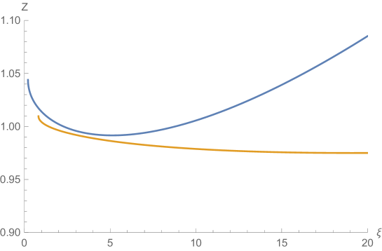
Figure 1: Dependence of the residue $Z$ for the Higgs field propagator on the gauge parameter $\xi$, for Region I (Blue), and Region II (Orange).

In FIG. 2, we find the spectral density functions both regions, for three values of $\xi:1,2,5$. Looking at Region I, we see the first two-particle state appearing at $t=(m_{h}+m_{h})^{2}=0.768\,\mu^{2}$, followed by another two-particle state at $t=(m+m)^{2}=0.922\,\mu^{2}$. Then, we see that there is a negative contribution, different for each diagram, at $t=(\sqrt{\xi}m+\sqrt{\xi}m)^{2}$. This corresponds to the (unphysical) two-particle state of two Goldstone bosons. For $\xi<3$, this leads to a negative contribution for the spectral function, probably due to the large-momentum behaviour of the Higgs propagator (24), for a detailed discussion see Dudal et al. (2019). For Region II, we find essentially the same behaviour: a Higgs two-particle state at $t=(m_{h}+m_{h})^{2}=0.81\,\mu^{2}$, and a gauge field two-particle state at $t=(m+m)^{2}=0.25\,\mu^{2}$. We also see a negative contribution different for each diagram at $t=(\sqrt{\xi}m+\sqrt{\xi}m)^{2}$, corresponding to the (unphysical) two-particle state of two Goldstone bosons.

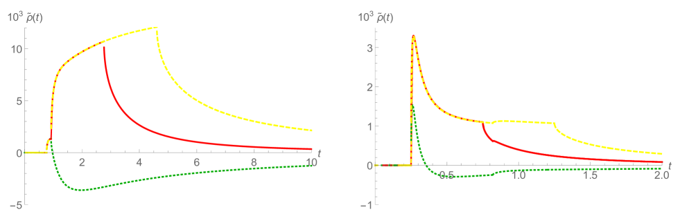
Figure 2: Spectral functions for the propagator $\langle h(p)h(-p)\rangle$, for $\xi=1$ (Green, Dotted), $\xi=3$ (Red, Solid), $\xi=5$ (Yellow, Dashed), with $t$ given in units of $\mu^{2}$, for Region I (left) and Region II (right) with the parameter values given in Table V A.

V.2.2 The transverse gauge field

For the gauge field propagator, following the steps from section V.1, we find the first-order pole mass of the transverse gauge field to be: for Region I

$$m_{\rm pole}^{2} = 0.274\,\mu^{2}$$ (89)

and for Region II

$$m_{\rm pole}^{2} = 0.065\,\mu^{2}$$ (90)

for all values of the parameter $\xi$, so that the pole mass is independent from the gauge parameter. The residue is, however, gauge dependent as is depicted in FIG. 3. For small values of $\xi$ the residue is not well-defined, as we will explain further in the next section.

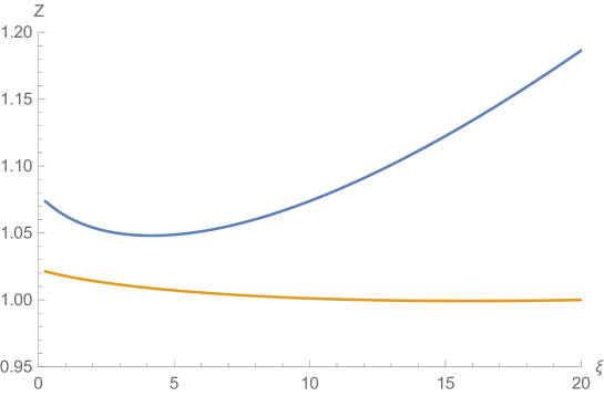
Figure 3: Dependence of the residue $Z$ for the gauge field propagator from the gauge parameter $\xi$, for Region I (Blue), and Region II (Orange).

In FIG. 4, we find the spectral density functions for both regions, for three values of $\xi$: $1,2,5$. Looking at Region I, we see the first two-particle state appearing at $t=(m_{h}+m)^{2}=0.843\,\mu^{2}$, followed by a two-particle state at $t=(m+m)^{2}=0.922\,\mu^{2}$. Then, we see that there is a negative contribution, different for each diagram, at $t=(m+\sqrt{\xi}m)^{2}$. This corresponds to the (unphysical) two-particle state of a gauge and Goldstone boson. For Region II, we find a gauge field two-particle state at $t=(m+m)^{2}=0.25\,\mu^{2}$. We also see a negative contribution different for each diagram at $t=(m+\sqrt{\xi}m)^{2}$, corresponding to the (unphysical) two-particle state of two Goldstone bosons.

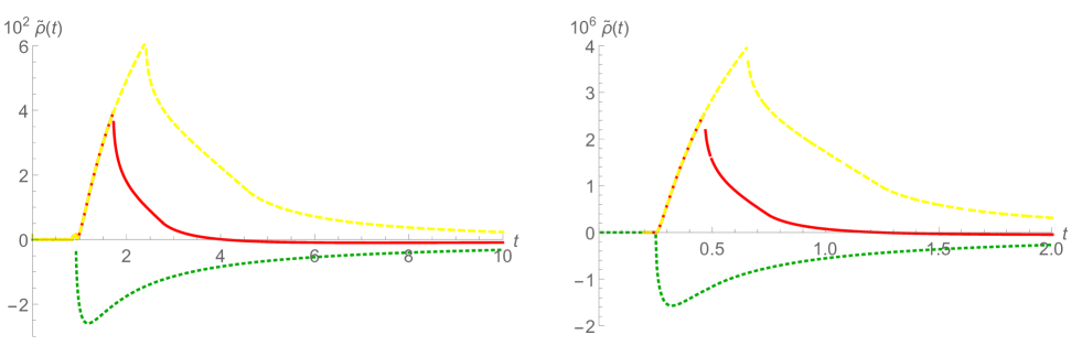
Figure 4: Spectral functions for the propagator $\langle A^{a}_{\mu}(p)A^{b}_{\nu}(-p)\rangle^{T}$, for $\xi=1$ (Green, Dotted), $\xi=3$ (Red, Solid), $\xi=5$ (Yellow, Dashed), with $t$ given in units of $\mu^{2}$, for Region I (left) and Region II (right) with the parameter values given in Table V A.

V.3 Unphysical threshold effects

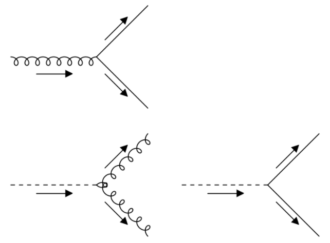
Figure 5: Possible decays of the gauge boson (above) and the Higgs boson (below). The arrows indicate the momentum flow.

From the Feynman vertex rules given in Appendix A, for certain values of the masses, unphysical threshold effects can occur. These effects imply that for certain values of the (physical and unphysical) parameters, a “decay” occurs of a gauge and Higgs boson into two other particles, see FIG. 5. We distinguish three cases:

• Decay of a gauge vector boson in two Goldstone bosons: this happens when $m>2\sqrt{\xi}m$.

• Decay of a Higgs boson in two gauge vector bosons: this happens when $m_{h}>2m$.

• Decay of a Higgs boson in two Goldstone bosons: this happens when $m_{h}>2\sqrt{\xi}m$.

In order to guarantee the stability of the gauge boson, we therefore need from $(1.)$ that $\xi>\frac{1}{4}$. This means that for the Landau gauge $\xi=0$, the elementary gauge boson is not stable. For the Higgs particle, to guarantee stability we need from $(2.)$ that $m_{h}<2m$. Then, from $(3.)$ we find that $\xi>\frac{m_{h}^{2}}{4m^{2}}$. This is the window in which we can work with a stable model. We can have a look at what happens when we go outside of this window. For the Higgs particle, we see that for $m_{h}>2m$, or $\lambda<g^{2}$, we will find a complex value for the first order pole mass, calculated through (75). For $\lambda\geq g^{2}$, we will always find a real pole mass. Since the pole mass is gauge invariant, we find that this is true for all values of $\xi$. However, we do find that for $\xi>\frac{m_{h}^{2}}{4m^{2}}$ and $\lambda>g^{2}$, the real value of the pole mass is a real point inside the branch cut. This means that we cannot achieve the usual differentiation around this point. As a consequence, we cannot consistently construct the residue, so that we are unable to obtain a first-order spectral function. For the gauge field, we find the same problem when $\xi<\frac{1}{4}$.

The foregoing mathematically correct observations clearly show that there is something physically wrong with using the elementary fields’ spectral functions. Luckily, all of these shortcomings are surpassed by using the gauge invariant composite operators.

V.4 Spectral properties for the composite fields

For the scalar composite operator ${O}(x)$, whose two-point function is given by expression (48), we find the first-order pole mass for Region I

$$m_{OO,\rm pole}^{2} = 0.207\,\mu^{2},$$ (91)

and for Region II

$$m_{OO,\rm pole}^{2} = 0.206\,\mu^{2},$$ (92)

which is equal to the pole mass of the elementary Higgs field in (87), as we expect from eq. (86). Following the steps from Section V.1, we find the first-order residue

$$Z=1.11\,v^{2}$$ (93)

for Region I and

$$Z=1.01\,v^{2}$$ (94)

for Region II. The first order spectral function for $\braket{O(x)\,O(y)}$ is shown in FIG. 6. Comparing this result with that of the spectral function of the Higgs field in FIG. 4, we see a two-particle state for the Higgs field at $t=(m_{h}+m_{h})^{2}$, and a two-particle state for the gauge vector field, starting at $t=(m+m)^{2}$. The difference is that for the gauge invariant correlation function $\braket{O(x)\,O(y)}$ we no longer have the unphysical Goldstone two-particle state. Due to the absence of this negative contribution, the spectral function is positive throughout the spectrum. In fact, we see that for bigger values of $\xi$, we find that the spectral function of the elementary Higgs field resembles more and more the spectral function of the composite operator $O(x)$. This makes sense, since for $\xi\rightarrow\infty$, we are approaching the unitary gauge which has a more direct link with the physical spectrum of the elementary excitations. In Appendix G, one finds a detailed discussion about the unitary gauge limit $\xi\rightarrow\infty$ as well as the calculation of the spectral function. Of course, the unitary gauge is not well-suited for computations at the quantum level due to the non-renormalizability issue in general, and non-curable overlapping divergences in particular, but for gauge invariant quantities, it was already noted in Irges and Koutroulis (2017) that (for the $\beta$-functions) the unitary gauge choice can still be useful, at least up to one-loop order. Therefore, in Appendix G, we have analyzed, at one-loop order where there are no overlapping divergences yet, the scalar and vector correlation functions directly in the unitary gauge and we do find that their finite pieces are identical to those obtained in the $R_{\xi}$-gauge discussed so far. Given that several propagators are trivial in the unitary gauge, the computations in the latter gauge are evidently far more economical. A similar observation was already made in the $U(1)$ case as well, see Capri et al. (2020).

The asymptotic (constant) behaviour is directly related to the (classical) dimension of the used composite operator.

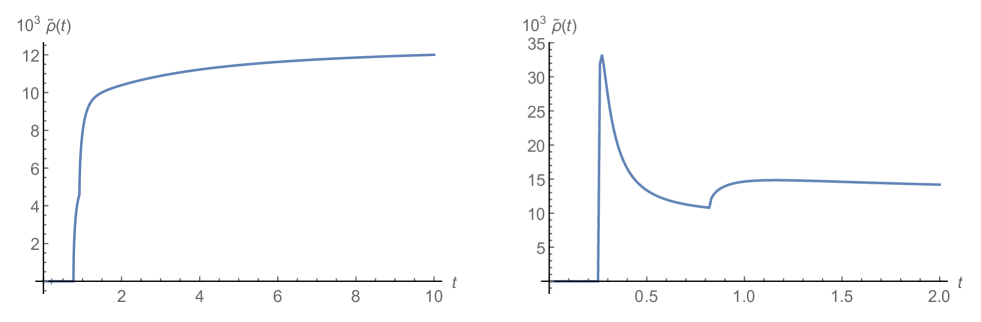
Figure 6: Spectral function for the two-point correlation function $\langle{O}(p){O}(-p)\rangle$, with $t$ given in units of $\mu^{2}$, for the Region I (left) and Region II (right) with parameter values given in Table V A.

V.4.1 The vector composite operator $R^{a}_{\mu}(x)$

For the transverse part of the two-point correlation function $G_{R}(p^{2})$, eq. (69), for our set of parameters we find the first-order pole mass: in Region I

$$m_{R,\rm pole}^{2} = 0.274\,\mu^{2}$$ (95)

and Region II

$$m_{R,\rm pole}^{2} = 0.065\,\mu^{2}$$ (96)

which is the same as the pole mass of the transverse gauge field, eq. (89), in agreement with eq. (86). Following the steps from V.1, we find the first-order residue

$$Z=\frac{1}{16}g^{2}v^{4}\left(1.27\right)$$ (97)

for Region I and

$$Z=\frac{1}{16}g^{2}v^{4}\left(1.05\right)$$ (98)

for Region II. The first order spectral function for $G_{R}(p^{2})$ is shown in FIG. 7. Comparing this to the spectral function of the gauge vector field in FIG. 4, we see a two-particle state at $t=(m_{h}+m)^{2}$, and a two-particle state for the gauge field, starting at $t=(m+m)^{2}$. Again, as in the case of the two-point correlation function of the scalar operator $O(x)$, the difference is that for this gauge invariant correlation function we no longer have the unphysical Goldstone/gauge boson two-particle state. Due to the absence of this negative contribution, the spectral function is positive throughout the spectrum. In fact, we see that for bigger values of $\xi$, we find that the spectral function of the elementary gauge field resembles more and more the spectral function of the composite operator $R^{a}_{\mu}(x)$. As already mentioned previously, this relies on the fact that in the limit $\xi\rightarrow\infty$ we are approaching the unitary gauge, see Appendix G. Also here, the linear increase at large $t$ follows from the operator dimension.

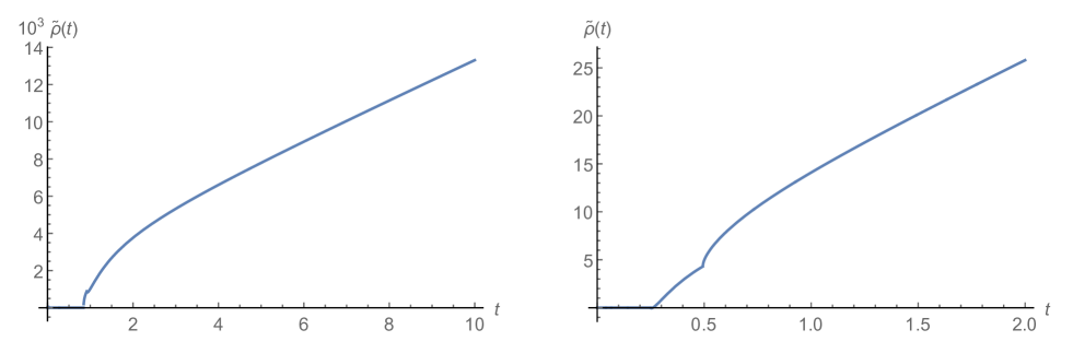
Figure 7: Spectral function for the transverse two-point correlation function $G_{R}(p^{2})$, with $t$ given in units of $\mu^{2}$, for the Region I (left) and Region II (right) with parameter values given in Table V A.

VI Conclusion and outlook

This work is the natural extension of previous studies Dudal et al. (2019, 2020a); Capri et al. (2020), where the Abelian $U(1)$ Higgs model has been scrutinized by employing two local composite BRST invariant operators ’t Hooft et al. (1980); Frohlich et al. (1980, 1981), whose two-point correlation functions provide a fully gauge independent description of the elementary excitations of the model, namely the Higgs and the massive gauge boson.

This formulation generalizes to the non-Abelian Higgs model as, for example, the $SU(2)$ Yang–Mills theory with a single Higgs in the fundamental representation ’t Hooft et al. (1980); Frohlich et al. (1980, 1981). This is the model which has been considered in the present analysis. The local gauge and BRST invariant composite operators $(O(x),R^{a}_{\mu}(x))$ which generalize their $U(1)$ counterparts are given in eq. (43) and in eqs. (56),(57).

The two-point correlation functions $\langle O(x)O(y)\rangle$ and $\langle R^{a}_{\mu}(x)R^{b}_{\nu}(y)\rangle^{T}$, where the superscript $T$ stands for the transverse component, have been evaluated at one-loop order in the $R_{\xi}$-gauge and compared with the corresponding correlation functions of the elementary fields $\langle h(x)h(y)\rangle$ and $\langle A^{a}_{\mu}(x)A^{b}_{\nu}(y)\rangle^{T}$. It turns out that both $\langle O(x)O(y)\rangle$ and $\langle h(x)h(y)\rangle$ share the same gauge independent pole mass, eqs.(87),(88),(91),(92), in agreement with both Nielsen identities Nielsen (1975); Piguet and Sibold (1985); Gambino et al. (1999); Gambino and Grassi (2000); Grassi et al. (2001); Aitchison and Fraser (1984); Andreassen et al. (2015) and the BRST invariant nature of $O(x)$. Nevertheless, unlike the residue and spectral function of the elementary correlator $\langle h(x)h(y)\rangle$, which exhibit a strong unphysical dependence from the gauge parameter $\xi$, FIG. 2, the spectral density of $\langle O(x)O(y)\rangle$ turns out to be $\xi$-independent and positive over the whole $p^{2}$ axis, FIG. 6. The same features hold for $\langle A^{a}_{\mu}(x)A^{b}_{\nu}(y)\rangle^{T}$ and $\langle R^{a}_{\mu}(x)R^{b}_{\nu}(y)\rangle^{T}$. Again, both correlation function share the same $\xi$-independent pole mass, eqs. (90),(90),(95),(96). Though, unlike the $\xi$-dependent spectral function associated to $\langle A^{a}_{\mu}(x)A^{b}_{\nu}(y)\rangle^{T}$, FIG. 4, that corresponding to $\langle R^{a}_{\mu}(x)R^{b}_{\nu}(y)\rangle^{T}$, FIG. 7, turns out to be independent from the gauge parameter $\xi$ and positive. As such, the local composite operators $(O(x),R^{a}_{\mu}(x))$ provide a fully BRST consistent description of the observable scalar (Higgs) and vector boson particles.

It is worth mentioning here that, besides the BRST invariance of the gauge fixed action, the model exhibits an additional global custodial symmetry, eqs.(20),(21), according to which all fields carrying the index $a=1,2,3$, i.e. $(A^{a}_{\mu},b^{a},c^{a},{\bar{c}}^{a},\rho^{a})$, undergo a global transformation in the adjoint representation of $SU(2)$. The same feature holds for the composite operators $(O(x),R^{a}_{\mu}(x))$ which transform exactly as $h$ and $A^{a}_{\mu}$. More precisely, the operator $O(x)$ is a singlet under the custodial symmetry, while the operators $R^{a}_{\mu}$ transform like a triplet, eq. (59), so that the correlation function $\langle R^{a}_{\mu}(p)R^{b}_{\nu}(-p)\rangle$ displays the same $SU(2)$ structure of the elementary two-point function $\langle A^{a}_{\mu}(p)A_{\nu}(-p)\rangle$, eqs.(60)-(63). Although not being the aim of the present analysis, we expect that the existence of a global custodial symmetry will imply far-reaching consequences for the renormalization properties of the composite operators $(O(x),R^{a}_{\mu}(x))$ encoded in the corresponding Ward identities, allowing a generalization of the $U(1)$ renormalizability analysis of Capri et al. (2020).

The analysis of the spectral properties of the operators $(O(x),R^{a}_{\mu}(x))$ worked out here could pave the route for more ambitious projects which might lead to an interesting interplay with possible future investigation on the lattice of the correlators $\langle O(x)O(y)\rangle$ and $\langle R^{a}_{\mu}(x)R^{b}_{\nu}(y)\rangle^{T}$, as already mentioned in Maas (2015, 2019). The BRST invariant nature of $(O(x),R^{a}_{\mu}(x))$ makes them natural candidates to attempting at facing the challenge of investigating the infrared non-perturbative behaviour of the model, trying to make contact with the analytical lattice predictions of Fradkin and Shenker Fradkin and Shenker (1979), see also Greensite (2011) for a general overview and Cherman et al. (2020) for a new take on these matters.. This study would enable us to shed some light on the issue of the positivity of the spectral densities in the non-perturbative region, a topic which is currently under intensive investigation in confining Yang–Mills theories without the presence of Higgs fields , see Oehme and Zimmermann (1980); Cornwall (1982); Zwanziger (1989); Alkofer and von Smekal (2001); Cucchieri et al. (2005); Bowman et al. (2007); Cucchieri and Mendes (2007); Aguilar et al. (2008); Dudal et al. (2008); Maas (2009); Fischer et al. (2009); Binosi and Papavassiliou (2009); Bogolubsky et al. (2009); Bornyakov et al. (2010); Cucchieri and Mendes (2010); Tissier and Wschebor (2010, 2011); Boucaud et al. (2012); Serreau and Tissier (2012); Oliveira and Silva (2012); Cornwall (2013); Aguilar et al. (2014); Peláez et al. (2014); Reinosa et al. (2015); Siringo (2016); Cyrol et al. (2016); Duarte et al. (2016); Reinosa et al. (2017); Frasca (2017); Lowdon (2018); Comitini and Siringo (2018); Huber (2018); Hayashi and Kondo (2019); Binosi and Tripolt (2020); Gracey et al. (2019); Kondo et al. (2020); Dudal et al. (2020b); Fischer and Huber (2020). Finally, it would be worth to investigate to which extent the BRST invariant correlation functions $\langle O(x)O(y)\rangle$, $\langle R^{a}_{\mu}(x)R^{b}_{\nu}(y)\rangle^{T}$ could be affected by the existence of the non-perturbative effect of the Gribov copies, by means of the recent BRST invariant formulation of the (Refined) Gribov-Zwanziger horizon function Capri et al. (2015, 2018).

Another most promising avenue to further explore is the $SU(2)\times U(1)$ setting of the electroweak theory, where the gauge invariant description of electric charge will necessitate the combination of the (local) gauge invariant composite operators set out here and (non-local) dressed gauge invariant operators, see Lavelle and McMullan (1997).

Appendix A Propagators and vertices

The tree level elementary propagators of the fields are easily computed, for example by coupling a source $J_{\varphi}$ to each field $\varphi$ and computing at leading order the functional derivative $\frac{\delta^{2}Z^{c}}{\delta J_{\varphi}(-p)\delta J_{\varphi}(p)}$ with $Z^{c}$ the generating functional of connected two-point functions. This leads to

$$\langle A^{a}_{\mu}(p)A^{b}_{\nu}(-p)\rangle = \frac{\delta^{ab}}{p^{2}+m^{2}}\mathcal{P}_{\mu\nu}(p)+\delta^{ab}\frac{\xi}{p^{2}+\xi m^{2}}\mathcal{L}_{\mu\nu}(p),$$

$$\langle\rho^{a}(p)\rho^{b}(-p)\rangle = \frac{\delta^{ab}}{p^{2}+\xi m^{2}},$$

$$\langle h(p)h(-p)\rangle = \frac{1}{p^{2}+m_{h}^{2}},$$

$$\langle A^{a}_{\mu}(p)b^{b}(-p)\rangle = \delta^{ab}\frac{p_{\mu}}{p^{2}+\xi m^{2}},$$

$$\langle b^{a}(p)\rho^{b}(-k)\rangle = \delta^{ab}\frac{im}{p^{2}+\xi m^{2}}$$ (99)

and

$$\langle\bar{c}^{a}(p)c^{b}(-p)\rangle = \frac{\delta^{ab}}{p^{2}+\xi m^{2}}$$ (100)

for the ghost propagator. All other propagators are zero. This includes the mixed propagator, $\braket{A_{\mu}^{a}(x)\rho^{b}(y)}=0$, a well-known feature of the $R_{\xi}$-gauge (Peskin and Schroeder, 1995, Chap. 21).

For all vertices, adopting the convention that the momentum is flowing towards the vertex, we get

• The $AAh$-vertex: $\Gamma_{A_{\mu}^{a}A_{\nu}^{b}h}(-p_{1},-p_{2},-p_{3})=-\frac{g^{2}v}{2}\delta_{\mu\nu}\delta^{ab}\delta(p_{1}+p_{2}+p_{3})$.

• The $\rho\rho A$-vertex: $\Gamma_{\rho^{a}\rho^{b}A_{\mu}^{c}}(-p_{1},-p_{2},-p_{3})=\frac{g}{2}i\epsilon^{abc}(p_{\mu,1}-p_{\mu,2})\delta(p_{1}+p_{2}+p_{3})$.

• The $A\rho h$-vertex: $\Gamma_{A_{\mu}^{a}\rho^{b}h}(-p_{1},-p_{2},-p_{3})=i\frac{g}{2}\delta^{ab}(p_{\mu,3}-p_{\mu,2})\delta(p_{1}+p_{2}+p_{3})$.

• The $hhh$ vertex: $\Gamma_{hhh}(-p_{1},-p_{2},-p_{3})=-3\lambda v\,\,\delta(p_{1}+p_{2}+p_{3})$.

• The $h\rho\rho$ vertex: $\Gamma_{h\rho^{a}\rho^{b}}(-p_{1},-p_{2},-p_{3})=-\lambda v\delta^{ab}\,\,\delta(p_{1}+p_{2}+p_{3})$.

• The $AAA$-vertex: $\Gamma_{A_{\mu}^{a}A_{\nu}^{b}A_{\sigma}^{c}}(-p_{1},-p_{2},-p_{3})=-igf^{abc}\left[(p_{1}-p_{3})_{\nu}\delta_{\sigma\mu}+(p_{3}-p_{2})_{\mu}\delta_{\nu\sigma}+(p_{2}-p_{1})_{\sigma}\delta_{\nu\mu}\right]\delta(p_{1}+p_{2}+p_{3})$.

• The $\overline{c}Ac$-vertex: $\Gamma_{\overline{c}^{a}A_{\mu}^{b}c^{c}}(-p_{1},-p_{2},-p_{3})=igf^{abc}p_{1,\mu}\delta(p_{1}+p_{2}+p_{3})$.

• The $AAAA$-vertex: $\Gamma_{A_{\mu}^{a}A_{\nu}^{b}A_{\rho}^{c}A_{\sigma}^{d}}(-p_{1},-p_{2},-p_{3},-p_{4})=g^{2}[f^{eab}f^{ecd}(\delta_{\mu\sigma}\delta_{\nu\rho}-\delta_{\mu\rho}\delta_{\nu\sigma})+f^{eac}f^{ebd}(\delta_{\mu\sigma}\delta_{\nu\rho}-\delta_{\mu\nu}\delta_{\rho\sigma})+f^{ead}f^{ebc}(\delta_{\mu\rho}\delta_{\nu\sigma}-\delta_{\mu\nu}\delta_{\rho\sigma})]\delta(p_{1}+p_{2}+p_{3}+p_{4})$.

• The $AAhh$-vertex: $\Gamma_{A_{\mu}^{a}A_{\nu}^{b}hh}(-p_{1},-p_{2},-p_{3},-p_{4})=-\frac{1}{2}g^{2}\delta^{ab}\delta_{\mu\nu}$.

• The $AA\rho\rho$-vertex: $\Gamma_{A_{\mu}^{a}A_{\nu}^{b}\rho^{c}\rho^{d}}(-p_{1},-p_{2},-p_{3},-p_{4})=-\frac{1}{2}g^{2}\delta_{\mu\nu}\delta^{ab}\delta^{cd}$.

Appendix B Custodial symmetry

The custodial symmetry given in Section II.2 is a result of the fact that the unbroken action is invariant under an $SU(2)_{\rm gauge}\times SU(2)_{\rm global}$ symmetry. This can be seen by writing $\Phi$ in the form of a bi-doublet Shifman (2012)

$$\Phi=\begin{pmatrix}\phi^{0*}&&\phi^{+}\\ -\phi^{+*}&&\phi^{0}\end{pmatrix}.$$ (101)

Clearly, the action,

$$\mathcal{L}_{\Phi} = \frac{1}{2}\text{Tr}\left(\mathcal{D}_{\mu}\Phi\right)^{\dagger}\left(\mathcal{D}_{\mu}\Phi\right)-\frac{\lambda}{4}\left(\text{Tr}\,\Phi^{\dagger}\Phi-v^{2}\right)^{2},$$ (102)

is invariant under the $SU(2)_{\rm gauge}\times SU(2)_{\rm global}$ transformation

$$\Phi \rightarrow U(x)\Phi M^{-1},$$

$$A_{\mu} \rightarrow U(x)A_{\mu}U^{-1}(x)+\frac{i}{g}U(x)\partial_{\mu}U^{-1}(x),$$ (103)

with $M$ an arbitrary $x$-independent matrix from $SU(2)_{\rm global}$. In the bidoublet notation, the expansion in eq. (8) becomes

$$\Phi = (h+v)\mathbf{1}+i\rho^{a}\tau^{a},$$ (104)

so the vev $\braket{\Phi}$ is not invariant under the transformation (103). However, it is invariant under the global diagonal $SU(2)\times SU(2)$ subgroup corresponding to $U(x)=M$. This is the custodial symmetry, given in infinitesimal form in eq. (20).

Appendix C Elementary propagators in the $R_{\xi}$-gauge

Here we will calculate the one-loop corrections to the Higgs and gauge field propagator. This requires the calculation of the Feynman diagrams as shown in FIGS. 8 and 9. To shorten the intermediate expressions, we will use the following functions:

$$\eta(m_{1},m_{2}) \equiv \frac{1}{(4\pi)^{d/2}}\Gamma(2-\frac{d}{2})\int_{0}^{1}dx\left(p^{2}x(1-x)+xm_{1}+(1-x)m_{2}\right)^{d/2-2},$$

$$\chi(m_{1}) \equiv \frac{1}{(4\pi)^{d/2}}\Gamma(1-\frac{d}{2})m_{1}^{d/2-1}.$$ (105)

Notice that the last four diagrams for both particles are zero for $\langle h\rangle=0$. In fact, including these diagrams has the same effect as making a shift in the vev of the scalar field $\Phi$ to demand $\langle h\rangle=0$, see the Appendix of Dudal et al. (2019) for the technical details. In the context of the FMS operators, we found it more convenient to expand around the (classical) $v$ that is gauge invariant, and thus to include the tadpoles. Expanding the FMS operator around the quantum corrected vev would lead to cancellations in that quantum vev coming from the propagator loop corrections to render it gauge invariant again, indeed the minimum of the quantum corrected effective Higgs potential is not gauge invariant itself.

C.0.1 Higgs propagator

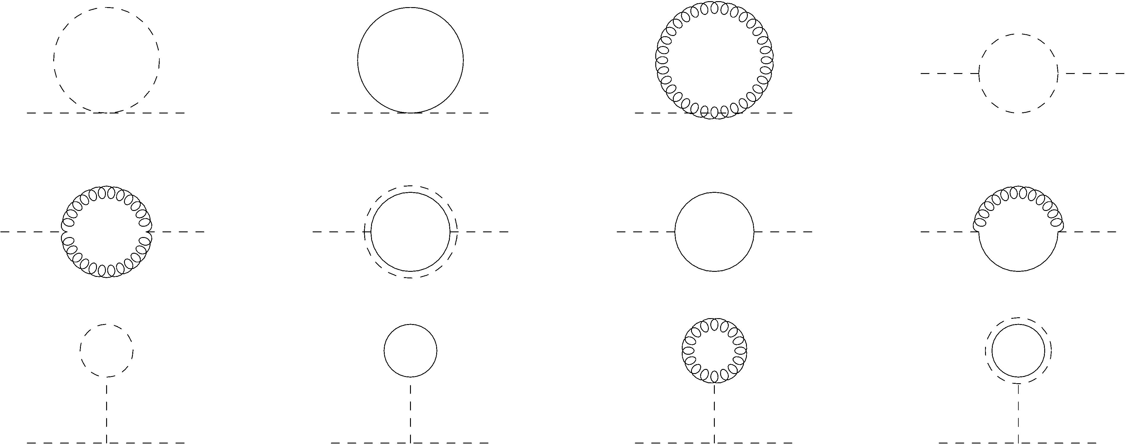
Figure 8: One-loop contributions to the propagator $\langle h(p)h(-p)\rangle$. Curly lines represent the gauge field, dashed lines the Higgs field, solid lines the Goldstone boson and double lines the ghost field.

The first diagrams contributing to the Higgs self-energy are of the snail type, renormalizing the masses of the internal fields. The Higgs boson snail (first diagram in the first line of FIG. 8):

$$\Gamma_{hh,1}(p^{2}) = -\frac{3\lambda\chi\left(m_{h}^{2}\right)}{2\left(m_{h}^{2}+p^{2}\right)^{2}},$$ (106)

the Goldstone boson snail (second diagram in the first line of FIG. 8):

$$\Gamma_{hh,2}(p^{2}) = -\frac{3\lambda\chi\left(m^{2}\xi\right)}{2\left(m_{h}^{2}+p^{2}\right)^{2}},$$ (107)

and the gauge field snail (third diagram in the first line of FIG. 8):

$$\Gamma_{hh,3}(p^{2}) = -\frac{3(d-1)g^{2}\chi\left(m^{2}\right)}{4\left(m_{h}^{2}+p^{2}\right)^{2}}-\frac{3g^{2}\xi\chi\left(m^{2}\xi\right)}{4\left(m_{h}^{2}+p^{2}\right)^{2}}.$$ (108)

Next, we meet a couple of sunset diagrams. The Higgs boson sunset (fourth diagram in the first line of FIG. 8):

$$\Gamma_{hh,4}(p^{2}) = \frac{9\lambda^{2}v^{2}\eta\left(m_{h}^{2},m_{h}^{2}\right)}{2\left(m_{h}^{2}+p^{2}\right)^{2}},$$ (109)

the gauge field sunset (first diagram in the second line of FIG. 8):

$$\Gamma_{hh,5}(p^{2}) = \frac{3g^{2}\eta\left(m^{2},m^{2}\right)\left(4(d-1)m^{4}+4m^{2}p^{2}+p^{4}\right)}{8m^{2}\left(m_{h}^{2}+p^{2}\right)^{2}}+\frac{3g^{2}\left(2m^{2}\xi+p^{2}\right)^{2}\eta\left(m^{2}\xi,m^{2}\xi\right)}{8m^{2}\left(m_{h}^{2}+p^{2}\right)^{2}}$$ (110)

$$- \frac{3g^{2}\left(m^{4}(\xi-1)^{2}+2m^{2}\xi p^{2}+2m^{2}p^{2}+p^{4}\right)\eta\left(m^{2},m^{2}\xi\right)}{4m^{2}\left(m_{h}^{2}+p^{2}\right)^{2}}+\frac{3g^{2}(\xi-1)\chi\left(m^{2}\right)}{4\left(m_{h}^{2}+p^{2}\right)^{2}}$$

$$- \frac{3g^{2}(\xi-1)\chi\left(m^{2}\xi\right)}{4\left(m_{h}^{2}+p^{2}\right)^{2}},$$

the ghost sunset (second diagram in the second line of FIG. 8):

$$\Gamma_{hh,6}(p^{2}) = -\frac{3g^{2}m^{2}\xi^{2}\eta\left(m^{2}\xi,m^{2}\xi\right)}{4\left(m_{h}^{2}+p^{2}\right)^{2}},$$ (111)

the Goldstone boson sunset (third diagram in the second line of FIG. 8):

$$\Gamma_{hh,7}(p^{2}) = \frac{3\lambda^{2}v^{2}\eta\left(m^{2}\xi,m^{2}\xi\right)}{2\left(m_{h}^{2}+p^{2}\right)^{2}},$$ (112)

and a mixed Goldstone-gauge sunset (fourth diagram in the second line of FIG. 8):

$$\Gamma_{hh,8}(p^{2}) = \frac{3g^{2}\left(\left(m^{2}(\xi-1)+p^{2}\right)^{2}+4m^{2}p^{2}\right)\eta\left(m^{2},m^{2}\xi\right)}{4m^{2}\left(m_{h}^{2}+p^{2}\right)^{2}}-\frac{3g^{2}\left(m^{2}\xi+p^{2}\right)^{2}\eta\left(m^{2}\xi,m^{2}\xi\right)}{4m^{2}\left(m_{h}^{2}+p^{2}\right)^{2}}$$ (113)

$$+ \frac{3g^{2}\chi\left(m^{2}\xi\right)\left(m^{2}(2\xi-1)+p^{2}\right)}{4m^{2}\left(m_{h}^{2}+p^{2}\right)^{2}}-\frac{3g^{2}\chi\left(m^{2}\right)\left(m^{2}(\xi-1)+p^{2}\right)}{4m^{2}\left(m_{h}^{2}+p^{2}\right)^{2}}.$$

Finally, we have the tadpole diagrams. The Higgs tadpole (first diagram on the third line of FIG. 8):

$$\Gamma_{hh,9}(p^{2}) = \frac{9\lambda^{2}v^{2}\chi\left(m_{h}^{2}\right)}{2m_{h}^{2}\left(m_{h}^{2}+p^{2}\right)^{2}},$$ (114)

the gauge tadpole (second diagram on the third line of FIG. 8):

$$\Gamma_{hh,10}(p^{2}) = \frac{9g\lambda mv\left((d-1)\chi\left(m^{2}\right)+\xi\chi\left(m^{2}\xi\right)\right)}{2m_{h}^{2}\left(m_{h}^{2}+p^{2}\right)^{2}},$$ (115)

the Goldstone boson tadpole (third diagram on the third line of FIG. 8):

$$\Gamma_{hh,11}(p^{2}) = \frac{9\lambda^{2}v^{2}\chi\left(m^{2}\xi\right)}{2m_{h}^{2}\left(m_{h}^{2}+p^{2}\right)^{2}},$$ (116)

the ghost tadpole (fourth diagram on the third line of FIG. 8):

$$\Gamma_{hh,12}(p^{2}) = -\frac{9g\lambda m\xi v\chi\left(m^{2}\xi\right)}{2m_{h}^{2}}.$$ (117)

Putting together eqs. (106) to (117) we find the Higgs up to first order in $\hbar$

$$\braket{h(x)\,h(y)} = \frac{1}{p^{2}+m_{h}^{2}}+g^{2}\Big{\{}\frac{3\left(4(d-1)m^{4}+4m^{2}p^{2}+p^{4}\right)}{8m^{2}}\eta\left(m^{2},m^{2}\right)$$ (118)

$$+ \frac{9m_{h}^{4}}{8m^{2}}\eta\left(m_{h}^{2},m_{h}^{2}\right)+\frac{3\left(m_{h}^{4}-p^{4}\right)}{8m^{2}}\eta\left(m^{2}\xi,m^{2}\xi\right)+\frac{\left(6(d-1)m^{2}-3p^{2}\right)}{4m^{2}}\chi\left(m^{2}\right)$$

$$+ \frac{3\left(m_{h}^{2}+p^{2}\right)}{4m^{2}}\chi\left(m^{2}\xi\right)+\frac{3m_{h}^{2}}{4m^{2}}\chi\left(m_{h}^{2}\right)\Big{\}}\frac{1}{(p^{2}+m_{h}^{2})^{2}}.$$

C.0.2 Gauge field propagator

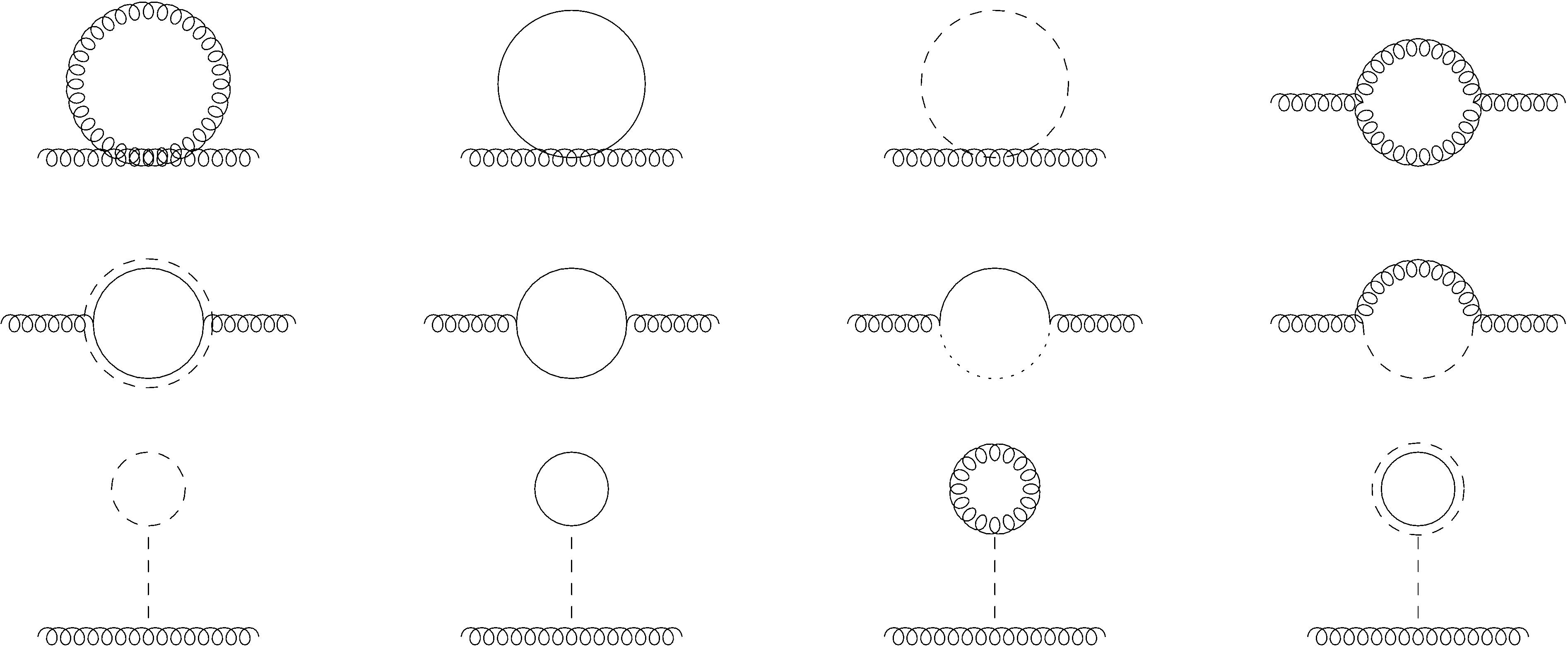
Figure 9: Contributions to the one-loop gauge field self-energy.

The first diagram contributing to transverse part of the gauge field self-energy is the gauge field snail (first diagram in the first line of FIG. 9) and gives a contribution:

$$\Pi_{AA^{T},1}(p^{2}) = \frac{2g^{2}\left(p^{2}-d\left(d^{2}-3d+3\right)p^{2}\right)\chi\left(m^{2}\right)}{(d-1)dp^{2}\left(m^{2}+p^{2}\right)^{2}}-\frac{2g^{2}\xi\left((d-2)dp^{2}+p^{2}\right)\chi\left(m^{2}\xi\right)}{(d-1)dp^{2}\left(m^{2}+p^{2}\right)^{2}}.$$ (119)

The second diagram is the Goldstone boson snail (second diagram in the first line of FIG. 9):

$$\Pi_{AA^{T},2}(p^{2}) = -\frac{3g^{2}\chi\left(m^{2}\xi\right)}{4\left(m^{2}+p^{2}\right)^{2}}.$$ (120)

The third diagram is the Higgs boson snail (third diagram in the first line of FIG. 9):

$$\Pi_{AA^{T},3}(p^{2}) = -\frac{g^{2}\chi\left(m_{h}^{2}\right)}{4\left(m^{2}+p^{2}\right)^{2}}.$$ (121)

The fourth diagram is the gauge field sunrise (fourth diagram in the first line of FIG. 9):

$$\Pi_{AA^{T},4}(p^{2}) = g^{2}\Big{\{}\frac{\eta\left(m^{2},m^{2}\xi\right)\left(2m^{2}p^{2}(-2d+\xi+3)+m^{4}(\xi-1)^{2}+p^{4}\right)}{2(d-1)m^{4}p^{2}}$$ (122)

$$- \frac{\left(4m^{2}+p^{2}\right)\eta\left(m^{2},m^{2}\right)\left(4(d-1)m^{4}+4(3-2d)m^{2}p^{2}+p^{4}\right)}{4(d-1)m^{4}\left(m^{2}+p^{2}\right)^{2}}$$

$$- \frac{\left(4m^{2}\xi p^{4}+p^{6}\right)\eta\left(m^{2}\xi,m^{2}\xi\right)}{4(d-1)m^{4}\left(m^{2}+p^{2}\right)^{2}}$$

$$+ \frac{\chi\left(m^{2}\xi\right)\left(4d^{2}\left(m^{2}(\xi+1)p^{2}+p^{4}\right)+d\left(m^{4}(\xi-1)-m^{2}(6\xi+7)p^{2}+(\xi-7)p^{4}\right)+4m^{2}\xi p^{2}\right)}{2(d-1)dm^{2}p^{2}\left(m^{2}+p^{2}\right)^{2}}$$

$$- \frac{\chi\left(m^{2}\right)\left(4d^{2}p^{4}+d\left(m^{4}(\xi-1)+m^{2}(2\xi-5)p^{2}+(\xi-7)p^{4}\right)+4m^{2}p^{2}\right)}{2(d-1)dm^{2}p^{2}\left(m^{2}+p^{2}\right)^{2}}\Big{\}}.$$

The fifth diagram is the ghost sunrise (first diagram in the second line of FIG. 9):

$$\Pi_{AA^{T},5}(p^{2}) = g^{2}\left\{\eta\left(m^{2}\xi,m^{2}\xi\right)\left(\frac{2m^{2}\xi}{(d-1)\left(m^{2}+p^{2}\right)^{2}}+\frac{p^{2}}{2(d-1)\left(m^{2}+p^{2}\right)^{2}}\right)-\frac{\chi\left(m^{2}\xi\right)}{(d-1)\left(m^{2}+p^{2}\right)^{2}}\right\}.$$ (123)

The sixth diagram is the Goldstone sunrise (second diagram in the second line of FIG. 9):

$$\Pi_{AA^{T},6}(p^{2}) = g^{2}\left\{\eta\left(m^{2}\xi,m^{2}\xi\right)\left(-\frac{m^{2}\xi}{(d-1)\left(m^{2}+p^{2}\right)^{2}}-\frac{p^{2}}{4(d-1)\left(m^{2}+p^{2}\right)^{2}}\right)+\frac{\chi\left(m^{2}\xi\right)}{2(d-1)\left(m^{2}+p^{2}\right)^{2}}\right\}.$$ (124)

The seventh diagram is the mixed Goldstone-Higgs sunrise (third diagram in the third line of FIG. 9):

$$\Pi_{AA^{T},7}(p^{2}) = g^{2}\left\{-\frac{\left(\left(-m_{h}^{2}+m^{2}\xi+p^{2}\right)^{2}+4m_{h}^{2}p^{2}\right)\eta\left(m_{h}^{2},m^{2}\xi\right)}{4(d-1)p^{2}\left(m^{2}+p^{2}\right)^{2}}+\frac{\chi\left(m_{h}^{2}\right)\left(-m_{h}^{2}+m^{2}\xi+p^{2}\right)}{4(d-1)p^{2}\left(m^{2}+p^{2}\right)^{2}}\right.$$ (125)

$$+ \left.\frac{\chi\left(m^{2}\xi\right)\left(m_{h}^{2}-m^{2}\xi+p^{2}\right)}{4(d-1)p^{2}\left(m^{2}+p^{2}\right)^{2}}\right\}.$$

The eighth diagram is the mixed Higgs-gauge field sunrise (fourth diagram in the second line of FIG. 9):

$$\Pi_{AA^{T},8}(p^{2}) = g^{2}\int_{0}^{1}dx\frac{\left(\left(m_{h}^{2}-m^{2}\xi+p^{2}\right)^{2}+4m^{2}\xi p^{2}\right)\eta\left(m_{h}^{2},m^{2}\xi\right)}{4(d-1)p^{2}\left(m^{2}+p^{2}\right)^{2}}-\frac{\eta\left(m^{2},m_{h}^{2}\right)\left(\left(m_{h}^{2}-m^{2}+p^{2}\right)^{2}-4(d-2)m^{2}p^{2}\right)}{4(d-1)p^{2}\left(m^{2}+p^{2}\right)^{2}}$$ (126)

$$- \frac{m^{2}(\xi-1)\chi\left(m_{h}^{2}\right)}{4(d-1)p^{2}\left(m^{2}+p^{2}\right)^{2}}-\frac{\chi\left(m^{2}\xi\right)\left(m_{h}^{2}-m^{2}\xi+p^{2}\right)}{4(d-1)p^{2}\left(m^{2}+p^{2}\right)^{2}}+\frac{\chi\left(m^{2}\right)\left(m_{h}^{2}-m^{2}+p^{2}\right)}{4(d-1)p^{2}\left(m^{2}+p^{2}\right)^{2}}.$$

Finally, we have four tadpole diagrams. The Higgs boson tadpole (first diagram of the third line in FIG. 9):

$$\Pi_{AA^{T},5}(p^{2}) = \frac{3gm\chi\left(m_{h}^{2}\right)}{2v\left(m^{2}+p^{2}\right)^{2}},$$ (127)

the Goldstone boson tadpole (second diagram of the last line in FIG. 9):

$$\Pi_{AA^{T},6}(p^{2}) = \frac{3g\lambda mv\chi\left(m^{2}\xi\right)}{2m_{h}^{2}\left(m^{2}+p^{2}\right)^{2}},$$ (128)

The gauge field tadpole (third diagram of the last line in FIG. 9):

$$\Pi_{AA^{T},7}(p^{2}) = \frac{3(d-1)g^{2}m^{2}\chi\left(m^{2}\right)}{2m_{h}^{2}\left(m^{2}+p^{2}\right)^{2}}+\frac{3g^{2}m^{2}\xi\chi\left(m^{2}\xi\right)}{2m_{h}^{2}\left(m^{2}+p^{2}\right)^{2}}$$ (129)

and finally, the ghost tadpole (fourth diagram of the last line in FIG. 9):

$$\Gamma_{AA^{T},8}(p^{2}) = -\frac{3g^{2}m^{2}\xi\chi\left(m^{2}\xi\right)}{2m_{h}^{2}\left(m^{2}+p^{2}\right)^{2}}.$$ (130)

Combining all these contributions (119)-(130), we find the total one-loop correction to the gauge field self-energy

$$\braket{A^{a}_{\mu}(p)A^{b}_{\nu}(p)}^{T} = \frac{\delta^{ab}}{p^{2}+m^{2}}+\delta^{ab}g^{2}\Big{\{}-\frac{\left(2(3-2d)m^{2}p^{2}+m_{h}^{4}-2m_{h}^{2}\left(m^{2}-p^{2}\right)+m^{4}+p^{4}\right)}{4(d-1)p^{2}}\eta\left(m^{2},m_{h}^{2}\right)$$ (131)

$$+ \frac{\left(m^{2}+p^{2}\right)^{2}\left(2m^{2}p^{2}(-2d+\xi+3)+m^{4}(\xi-1)^{2}+p^{4}\right)}{2(d-1)m^{4}p^{2}}\eta\left(m^{2},m^{2}\xi\right)$$

$$+ \frac{\left(m^{4}-p^{4}\right)\left(4m^{2}\xi+p^{2}\right)}{4(d-1)m^{4}}\eta\left(m^{2}\xi,m^{2}\xi\right)-\frac{\left(4m^{2}+p^{2}\right)\left(4(d-1)m^{4}+4(3-2d)m^{2}p^{2}+p^{4}\right)}{4(d-1)m^{4}}\eta\left(m^{2},m^{2}\right)$$

$$+ \frac{\left(m_{h}^{2}\left(-m^{2}p^{2}\left(8d^{2}-24d+4\xi+13\right)-2p^{4}(4d+\xi-7)+m^{4}(1-2\xi)\right)+6(d-1)^{2}m^{4}p^{2}+m_{h}^{4}m^{2}\right)}{4(d-1)m_{h}^{2}m^{2}p^{2}}\chi\left(m^{2}\right)$$

$$- \frac{\left((d-2)p^{2}+m_{h}^{2}-m^{2}\right)}{4(d-1)p^{2}}\chi\left(m_{h}^{2}\right)+\frac{\left(m^{2}p^{2}(5d+4\xi-13)+2p^{4}(4d+\xi-7)+2m^{4}(\xi-1)\right)}{4(d-1)m^{2}p^{2}}\chi\left(m^{2}\xi\right)$$

$$+ \frac{3}{4}\chi\left(m_{h}^{2}\right)+\frac{3}{4}\chi\left(m^{2}\xi\right)\Big{\}}\frac{1}{(p^{2}+m^{2})^{2}}.$$

Appendix D Contributions to $\langle O(p)O(-p)\rangle$ in the $R_{\xi}$-gauge

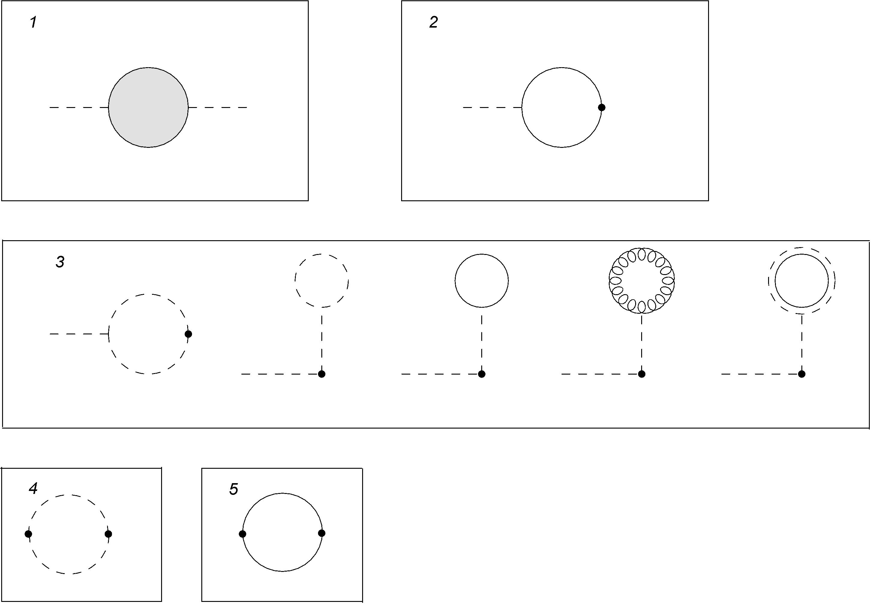
Figure 10: One-loop contributions for the propagator $\langle O(x)O(y)\rangle$. Curly lines represent the gauge field, dashed lines the Higgs field, solid lines the Goldstone boson and double lines the ghost field. The $\bullet$ indicates the insertion of a composite operator.

.

The diagrams which contribute to the correlation function $\langle O(p)O(-p)\rangle$ are depicted in FIG. 10. The first term (first box in FIG. 10) is $v^{2}$ times the one-loop correction to the Higgs propagator, given in eq. (118). The second term (second box in FIG. 10) is

$$v\langle h(p)(\rho^{a}\rho^{a})(-p)\rangle = -3\frac{m_{h}^{2}\eta\left(m^{2}\xi,m^{2}\xi\right)}{m_{h}^{2}+p^{2}}.$$ (132)

The third term (third box in FIG. 10) is

$$v\langle h(p)h^{2}(-p)\rangle = -\frac{3m_{h}^{2}\eta\left(m_{h}^{2},m_{h}^{2}\right)}{m_{h}^{2}+p^{2}}-\frac{3\chi\left(m_{h}^{2}\right)}{m_{h}^{2}+p^{2}}-\frac{\chi\left(m^{2}\xi\right)}{m_{h}^{2}+p^{2}}-\frac{2(d-1)m^{2}\chi\left(m^{2}\right)}{m_{h}^{2}\left(m_{h}^{2}+p^{2}\right)}-\frac{2m^{2}\xi\chi\left(m^{2}\xi\right)}{m_{h}^{2}\left(m_{h}^{2}+p^{2}\right)}$$ (133)

$$+ \frac{2m^{2}\xi\chi\left(m^{2}\xi\right)}{m_{h}^{2}\left(m_{h}^{2}+p^{2}\right)}.$$

The fourth term (fourth box in FIG. 10) is

$$\langle m_{h}^{2}(p)m_{h}^{2}(-p)\rangle = \frac{1}{2}\eta\left(m_{h}^{2},m_{h}^{2}\right).$$ (134)

The fifth term (fifth box in FIG. 10) is

$$\langle(\rho^{a}\rho^{a})(p)(\rho^{b}\rho^{b})(-p)\rangle = \frac{3}{2}\eta\left(\xi m^{2},\xi m^{2}\right)$$ (135)

and together these terms give the correlation function of the scalar composite operator $O(p)$ up to first order in $\hbar$

$$\langle O(p)O(-p)\rangle = \frac{v^{2}}{p^{2}+m_{h}^{2}}+\Big{\{}\frac{3}{2}\eta\left(m^{2},m^{2}\right)(4(d-1)m^{4}+4m^{2}p^{2}+p^{4})+\frac{1}{2}(p^{2}-2m_{h}^{2})^{2}\eta\left(m_{h}^{2},m_{h}^{2}\right)$$ (136)

$$- \frac{3p^{2}\chi(m^{2})(2(d-1)m^{2}+m_{h}^{2})}{m_{h}^{2}}-3p^{2}\chi(m_{h}^{2})\Big{\}}\frac{1}{(p^{2}+m_{h}^{2})^{2}}.$$

Appendix E Contributions to $\langle R_{\mu}^{a}(p)R_{\nu}^{a}(-p)\rangle$ in the $R_{\xi}$-gauge

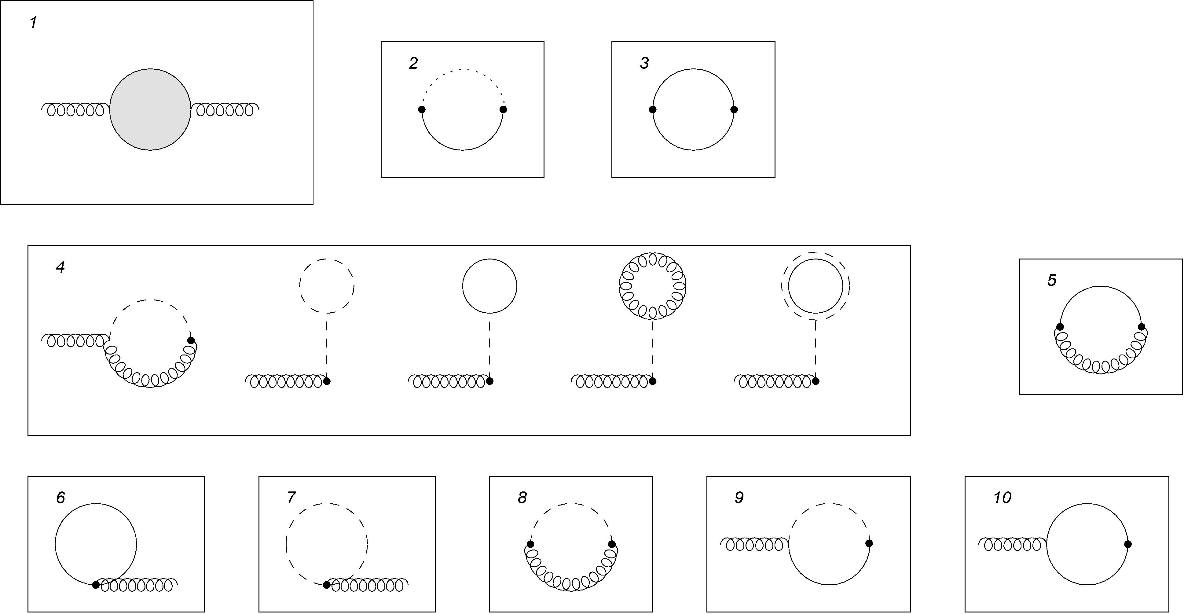
Figure 11: One-loop contributions for the propagator $\langle R^{a}_{\mu}(x)R^{a}_{\nu}(y)\rangle$ in the unitary gauge. Curly lines represent the gauge field, dashed lines the Higgs field, solid lines the Goldstone boson and double lines the ghost field. The $\bullet$ indicates the insertion of a composite operator.

.

The diagrams which contribute to the correlation function $\langle R_{\mu}^{a}(p)R_{\nu}^{a}(-p)\rangle$ are depicted in FIG. 11. The first term (first box in FIG. 11) is $\frac{1}{16}g^{2}v^{4}$ times the one-loop corrected function, given by eq. (131). The second term (second box in FIG. 11) is

$$-\left\langle\rho^{a}(p)\partial_{\mu}h(p),\partial_{\nu}\rho^{a}(-p)h(-p)\right\rangle = \frac{3}{4(d-1)p^{2}}\Bigg{\{}\chi\left(m^{2}\xi\right)\left(m_{h}^{2}+p^{2}-m^{2}\xi\right)-\left(4m_{h}^{2}p^{2}+\left(-m_{h}^{2}+m^{2}\xi+p^{2}\right)^{2}\right)\eta\left(m_{h}^{2},m^{2}\xi\right)$$ (137)

$$\,-\chi\left(m_{h}^{2}\right)\left(m_{h}^{2}-m^{2}\xi-p^{2}\right)\Bigg{\}}\mathcal{P}_{\mu\nu}(p).$$

The third term (third box in FIG. 11) is

$$-\frac{1}{2}\left\langle\rho^{a}(x)\partial_{\mu}\rho^{b}(x),\partial_{\nu}\rho^{a}(y)\rho^{b}(y)\right\rangle=\left\{\frac{3\chi\left(m^{2}\xi\right)}{2(d-1)}-\frac{3\left(4m^{2}\xi+p^{2}\right)\eta\left(m^{2}\xi,m^{2}\xi\right)}{4(d-1)}\right\}\mathcal{P}_{\mu\nu}(p).$$ (138)

The fourth term (fourth box in FIG. 11)is

$$\frac{1}{4}g^{2}v^{3}\left\langle A_{\mu}^{a}(x),A_{\nu}^{a}(y)h(y)\right\rangle = \left\{-\frac{3m^{2}\left(\left(-m_{h}^{2}+m^{2}\xi+p^{2}\right)^{2}+4m_{h}^{2}p^{2}\right)\eta\left(m_{h}^{2},m^{2}\xi\right)}{2(d-1)p^{2}\left(m^{2}+p^{2}\right)}\right.$$ (139)

$$+\frac{3m^{2}\eta\left(m^{2},m_{h}^{2}\right)\left(4p^{2}\left(m_{h}^{2}-(d-1)m^{2}\right)+\left(-m_{h}^{2}+m^{2}+p^{2}\right)^{2}\right)}{2(d-1)p^{2}\left(m^{2}+p^{2}\right)}$$

$$+\frac{3m^{2}\chi\left(m^{2}\xi\right)\left(\frac{m_{h}^{2}-m^{2}\xi+p^{2}}{(d-1)p^{2}}-3\right)}{2\left(m^{2}+p^{2}\right)}+\frac{3m^{4}\chi\left(m_{h}^{2}\right)\left(\frac{\xi-1}{(d-1)p^{2}}-\frac{3}{m^{2}}\right)}{2\left(m^{2}+p^{2}\right)}$$

$$\left.-\frac{3m^{2}\chi\left(m^{2}\right)\left(6(d-1)^{2}m^{2}p^{2}+m_{h}^{4}+m_{h}^{2}\left(p^{2}-m^{2}\right)\right)}{2(d-1)m_{h}^{2}p^{2}\left(m^{2}+p^{2}\right)}\right\}\mathcal{P}_{\mu\nu}(p).$$

The fifth term (fifth box in FIG. 11) is

$$\frac{1}{6}g^{2}v^{2}\left\langle\rho^{a}(x)A_{\mu}^{b}(x),\rho^{a}(y)A_{\nu}^{b}(y)\right\rangle = \Bigg{\{}-\frac{3\left(\left(m^{2}(\xi-1)+p^{2}\right)^{2}-4(d-2)m^{2}p^{2}\right)\eta\left(m^{2},m^{2}\xi\right)}{2(d-1)p^{2}}$$ (140)

$$+ \frac{3\left(4m^{2}\xi+p^{2}\right)\eta\left(m^{2}\xi,m^{2}\xi\right)}{2(d-1)}+\frac{3\chi\left(m^{2}\right)\left(m^{2}(\xi-1)+p^{2}\right)}{2(d-1)p^{2}}$$

$$- \frac{3\chi\left(m^{2}\xi\right)\left(m^{2}(\xi-1)+p^{2}\right)}{2(d-1)p^{2}}\Bigg{\}}\mathcal{P}_{\mu\nu}(p)$$

The sixth term is

$$-\frac{1}{24}g^{2}v^{2}\left\langle\rho^{a}(x)\rho^{a}(x)A_{\mu}^{b}(x),A^{b}(y)\right\rangle=-\frac{3g^{2}v^{2}\chi\left(\xi m^{2}\right)}{8\left(m^{2}+p^{2}\right)}\mathcal{P}_{\mu\nu}(p).$$ (141)

The seventh term (seventh box in FIG. 11) is

$$\frac{1}{8}g^{2}v^{2}\left\langle h(x)h(x)A_{\mu}^{a}(x),A_{\nu}^{a}(y)\right\rangle=\frac{3g^{2}v^{2}\chi\left(m_{h}^{2}\right)}{8\left(m^{2}+p^{2}\right)}\mathcal{P}_{\mu\nu}(p).$$ (142)

The eighth term (eighth box in FIG. 11) is

$$\frac{1}{4}g^{2}v^{2}\left\langle h(x)A_{\mu}^{a}(x),h(y)A_{\nu}^{a}(y)\right\rangle = 3m^{2}\left\{\frac{\left(\left(-m_{h}^{2}+m^{2}\xi+p^{2}\right)^{2}+4m_{h}^{2}p^{2}\right)\eta\left(m_{h}^{2},m^{2}\xi\right)}{4(d-1)m^{2}p^{2}}\right.$$ (143)

$$-\frac{\eta\left(m^{2},m_{h}^{2}\right)\left(4p^{2}\left(m_{h}^{2}-(d-1)m^{2}\right)+\left(-m_{h}^{2}+m^{2}+p^{2}\right)^{2}\right)}{4(d-1)m^{2}p^{2}}$$

$$+\frac{\chi\left(m^{2}\xi\right)\left(-m_{h}^{2}+m^{2}\xi-p^{2}\right)}{4(d-1)m^{2}p^{2}}+\frac{\chi\left(m^{2}\right)\left(m_{h}^{2}-m^{2}+p^{2}\right)}{4(d-1)m^{2}p^{2}}$$

$$\left.-\frac{(\xi-1)\chi\left(m_{h}^{2}\right)}{4(d-1)p^{2}}\right\}\mathcal{P}_{\mu\nu}(p).$$

The ninth term (ninth box in FIG. 11) is

$$\frac{1}{2}gv^{2}\left\langle\partial_{\mu}h(x)\rho^{a}(x),A_{\nu}^{a}(y)\right\rangle = -\frac{3}{2}g^{2}v^{2}\left\{-\frac{\left(\left(-m_{h}^{2}+m^{2}\xi+p^{2}\right)^{2}+4m_{h}^{2}p^{2}\right)\eta\left(m_{h}^{2},m^{2}\xi\right)}{4(d-1)p^{2}\left(m^{2}+p^{2}\right)}\right.$$ (144)

$$\left.+\frac{\chi\left(m_{h}^{2}\right)\left(-m_{h}^{2}+m^{2}\xi+p^{2}\right)}{4(d-1)p^{2}\left(m^{2}+p^{2}\right)}+\frac{\chi\left(m^{2}\xi\right)\left(m_{h}^{2}-m^{2}\xi+p^{2}\right)}{4(d-1)p^{2}\left(m^{2}+p^{2}\right)}\right\}\mathcal{P}_{\mu\nu}(p).$$

The tenth term (tenth box in FIG. 11) is

$$-\frac{1}{4}gv^{2}\varepsilon^{abc}\left\langle A^{a}(x),\rho^{b}\partial_{\mu}\rho^{c}\right\rangle=-\frac{3}{4}g^{2}v^{2}\left\{\frac{\left(4m^{2}\xi p^{2}+p^{4}\right)\eta\left(m^{2}\xi,m^{2}\xi\right)}{2(d-1)p^{2}\left(m^{2}+p^{2}\right)}-\frac{\chi\left(m^{2}\xi\right)}{(d-1)\left(m^{2}+p^{2}\right)}\right\}\mathcal{P}_{\mu\nu}(p)$$ (145)

and together these terms give the transverse part of the correlation function of the scalar composite operator $R^{a}_{\mu}$ up to first order in $\hbar$

$$\left\langle R_{\mu}^{a}(x),R_{\nu}^{a}(y)\right\rangle^{T} = \frac{3}{16}g^{2}v^{4}\frac{1}{p^{2}+m^{2}}-3\left\{-\frac{p^{2}\left(2(3-2d)m^{2}p^{2}-2m_{h}^{2}\left(m^{2}-p^{2}\right)+m_{h}^{4}+m^{4}+p^{4}\right)}{4(d-1)}\eta\left(m^{2},m_{h}^{2}\right)\right.$$ (146)

$$-\frac{\left(4m^{2}+p^{2}\right)\left(4(d-1)m^{4}+4(3-2d)m^{2}p^{2}+p^{4}\right)}{4(d-1)}\eta\left(m^{2},m^{2}\right)$$

$$+\frac{\chi\left(m^{2}\right)\left(m_{h}^{2}\left(-8\left(d^{2}-3d+2\right)m^{4}+(15-8d)m^{2}p^{2}+3p^{4}\right)-6(d-1)^{2}m^{4}\left(m^{2}+2p^{2}\right)+p^{2}m_{h}^{4}\right)}{4(d-1)m_{h}^{2}}$$

$$\left.+\frac{\chi\left(m_{h}^{2}\right)\left(-2(d-1)m^{4}+(5-4d)m^{2}p^{2}-p^{2}m_{h}^{2}+p^{4}\right)}{4(d-1)}\right\}\frac{1}{\left(m^{2}+p^{2}\right)^{2}}.$$

Appendix F Fundamental Feynman integral

$$\int_{0}^{1}dx\ln\frac{p^{2}x(1-x)+xm_{1}^{2}+(1-x)m_{2}^{2}}{\mu^{2}}=-2 + \frac{1}{2p^{2}}\Bigg{\{}m_{1}^{2}\ln(\frac{m_{2}^{2}}{m_{1}^{2}})+m_{2}^{2}\ln(\frac{m_{1}^{2}}{m_{2}^{2}})+p^{2}\ln(\frac{m_{1}^{2}m_{2}^{2}}{\mu^{4}})$$ (147)

$$- 2\sqrt{-m_{1}^{4}+2m_{1}^{2}m_{2}^{2}-2m_{1}^{2}p^{2}-m_{2}^{4}-2m_{2}^{2}p^{2}-p^{4}}$$

$$\times \tan^{-1}\Big{[}\frac{-m_{1}^{2}+m_{2}^{2}-p^{2}}{\sqrt{-m_{1}^{4}+2m_{1}^{2}(m_{2}^{2}-p^{2})-(m_{2}^{2}+p^{2})^{2}}}\Big{]}$$

$$+ 2\sqrt{-m_{1}^{4}+2m_{1}^{2}m_{2}^{2}-2m_{1}^{2}p^{2}-m_{2}^{4}-2m_{2}^{2}p^{2}-p^{4}}$$

$$\times \tan^{-1}\Big{[}\frac{-m_{1}^{2}+m_{2}^{2}+p^{2}}{\sqrt{-m_{1}^{4}+2m_{1}^{2}(m_{2}^{2}-p^{2})-(m_{2}^{2}+p^{2})^{2}}}\Big{]}\Bigg{\}}.$$

Appendix G A digression on the unitary gauge

It is well-known that in the unitary gauge the unphysical fields, like the Goldstone and ghost fields, decouple, a feature which allows for a more direct link with the spectrum of the elementary excitations of the model. However, this gauge is known to be non-renormalizable. In fact, working directly with the elementary tree level propagators taken a priori in the unitary limit, i.e. $\xi\rightarrow\infty$, and following the steps of dimensional regularization, we find that the divergent part of the inverse Higgs propagator reads

$$G^{-1}_{hh,\rm div}(p^{2}) = \frac{3g^{2}\left(m_{h}^{4}+6m^{2}p^{2}+p^{4}\right)}{64\pi^{2}m^{2}\epsilon}.$$ (148)

We used here that the surviving tree level propagators in the unitary gauge are

$$\langle A^{a}_{\mu}(p)A^{b}_{\nu}(-p)\rangle = \frac{\delta^{ab}}{p^{2}+m^{2}}\mathcal{P}_{\mu\nu}(p)+\delta^{ab}\frac{1}{m^{2}}\mathcal{L}_{\mu\nu}(p)=\frac{\delta^{ab}}{p^{2}+m^{2}}\Big{(}\delta_{\mu\nu}+\frac{p_{\mu}p_{\nu}}{m^{2}}\Big{)},$$

$$\langle h(p)h(-p)\rangle = \frac{1}{p^{2}+m_{h}^{2}}\,$$ (149)

with all other propagators, i.e. the Goldstone and Faddeev-Popov ghost propagators, vanishing. In expression (148) we clearly see the presence of the term $\sim\frac{p^{4}}{\epsilon m^{2}}$, signalling the aforementioned issue of the non-renormalizability. In essence, this can be traced back to the tree level presence of $\frac{p_{\mu}p_{\nu}}{m^{2}}$, a non power-counting controllable term.

Nevertheless, it is interesting to observe that, if we remove the divergent part (148) anyway, we obtain the spectral function as shown in FIG. 12. This spectral function is almost identical to that obtained for the composite operator $O(x)$, see FIG. 6.

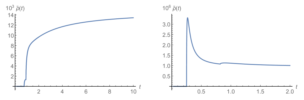
Figure 12: Spectral function for the propagator $\langle h(p)h(-p)\rangle$ in the unitary gauge, with $t$ given in unity of $\mu^{2}$, for the Region I (left) and Region II (right), with parameter values given in Table V A.

For the inverse gauge field propagator, proceeding in the same way, we find the divergent part

$$G^{-1}_{AA,\rm div}(p^{2}) = \frac{1}{\epsilon}\Big{(}-\frac{9g^{2}m^{4}}{16\pi^{2}m_{h}^{2}}-\frac{g^{2}p^{6}}{96\pi^{2}m^{4}}+\frac{7g^{2}p^{4}}{48\pi^{2}m^{2}}+\frac{3g^{2}m^{2}}{32\pi^{2}}+\frac{83g^{2}p^{2}}{96\pi^{2}}-\frac{3\lambda m^{2}}{8\pi^{2}}\Big{)}$$ (150)

which shows again the non-renormalizability of unitary gauge, through the terms $\sim\frac{p^{6}}{\epsilon m^{4}}$ and $\sim\frac{p^{4}}{\epsilon m^{2}}$ . However, if we remove also here those terms by hand, we obtain the spectral function as shown in FIG. 13.

Apart from the by hand removal of the divergences in this unitary gauge exercise, the nice behaviour of the spectral densities for the Higgs and gauge field obtained by a direct use of the tree level propagators already taken in the unitary limit, $\xi\rightarrow\infty$, can be, to some extent, justified by the fact that we are working at the one-loop order in perturbation theory. Since overlapping divergences start from two-loop onward, we can easily figure out that the naive use of the elementary tree level propagators taken already in the unitary limit will run into severe non-renormalizibility issues, making the removal of the (overlapping) divergent parts (148), (150) quite problematic beyond the current one-loop level.

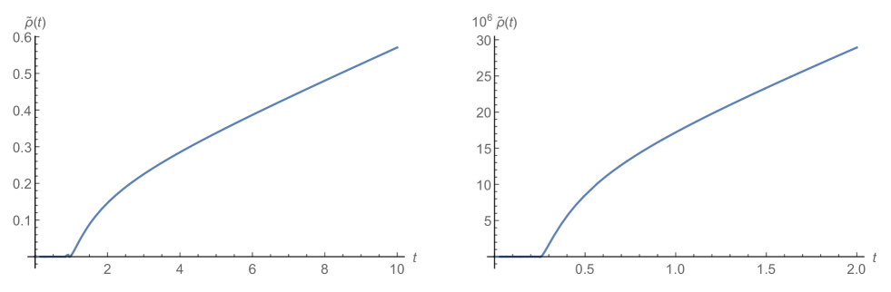
Figure 13: Spectral function for the propagator $\langle A^{a}_{\mu}(p)A^{b}_{\nu}(-p)\rangle$ in the unitary gauge, with $t$ given in unity of $\mu^{2}$, for the Region I (left) and Region II (right), with parameter values given in Table V A.

Now for what concerns the composite operators, since $O(x)$ is BRST invariant, any choice for the gauge fixing should give the same expression for the correlation function $G_{OO}(p^{2})$. So again using the unitary gauge, eq. (44) simplifies to

$$\braket{{O}(x){O}(y)}_{\rm unitary} = v^{2}\braket{h(x)h(y)}_{\rm unitary}+v\braket{h(x)h(y)^{2}}_{\rm unitary}+\frac{1}{4}\braket{h(x)^{2}h(y)^{2}}_{\rm unitary},$$ (151)

with the consecutive terms displayed diagrammatically by the respective boxes in FIG. 14. Using dimensional regularization in the $\overline{\mbox{MS}}$-scheme with $(d=4-\epsilon)$ and switching to momentum space, we find

$$v^{2}\braket{h(p)h(-p)}_{\rm unitary} = \frac{3}{32\pi^{2}}\int_{0}^{1}dx\Bigg{\{}\frac{1}{\epsilon}\left(2m_{h}^{4}+12m^{2}p^{2}+2p^{4}\right)+2m_{h}^{4}\ln\left(\frac{m_{h}^{2}}{\mu^{2}}\right)+2\left(6m^{4}-m^{2}p^{2}\right)\ln\left(\frac{m^{2}}{\mu^{2}}\right)$$ (152)

$$- 3m_{h}^{4}\ln\left(\frac{p^{2}(1-x)x+m_{h}^{2}}{\mu^{2}}\right)-\left(12m^{4}+4m^{2}p^{2}+p^{4}\right)\ln\left(\frac{p^{2}(1-x)x+m^{2}}{\mu^{2}}\right)$$

$$- 2m_{h}^{4}+2m^{2}\left(p^{2}-6m^{2}\right)\Bigg{\}}\frac{1}{\left(m_{h}^{2}+p^{2}\right){}^{2}},$$

$$v\braket{h(p)h(-p)^{2}}_{\rm unitary} = \frac{3}{16\pi^{2}m_{h}^{2}}\int_{0}^{1}dx\Bigg{\{}\frac{12}{\epsilon}m^{4}-6m^{4}\ln\left(\frac{m^{2}}{\mu^{2}}\right)-m_{h}^{4}\ln\left(\frac{m_{h}^{2}}{\mu^{2}}\right)$$ (153)

$$+ m_{h}^{4}\ln\left(\frac{m_{h}^{2}+p^{2}(1-x)x}{\mu^{2}}\right)+m_{h}^{4}+2m^{4}\Bigg{\}}\frac{1}{\left(m_{h}^{2}+p^{2}\right)},$$

$$\frac{1}{4}\braket{h(p)^{2}h(p)^{2}}_{\rm unitary} = \frac{1}{16\pi^{2}}\int_{0}^{1}dx\Bigg{\{}\frac{1}{\epsilon}-\frac{1}{2}\ln\left(\frac{m_{h}^{2}+p^{2}(1-x)x}{\mu^{2}}\right)\Bigg{\}}.$$ (154)

Inserting now the unity

$$1=(p^{2}+m_{h}^{2})/(p^{2}+m_{h}^{2})=((p^{2}+m_{h}^{2})/(p^{2}+m_{h}^{2}))^{2},$$ (155)

we find indeed that the finite pieces of $\braket{O(x)O(y)}_{\rm unitary}$ and $\braket{O(x)O(y)}_{R_{\xi}}$ do coincide, this is evidently related to the gauge invariance. From two-loop onward the overlapping divergences will show up again, requiring a fully renormalizable setup.

Figure 14: One-loop contributions for the propagator $\langle O(x)O(y)\rangle$ in the unitary gauge. Curly lines represent the gauge field and dashed lines the Higgs field. The $\bullet$ indicates the insertion of a composite operator.

.

We can stretch the unitary gauge even a bit further, to also look at the vector correlator, $\braket{R^{a}_{\mu}(p)\,R^{a}_{\nu}(-p)}_{\rm unitary}$. We find at one-loop order

$$\braket{R^{a}_{\mu}(p)\,R^{a}_{\nu}(-p)} = \frac{1}{16}g^{2}v^{4}\langle A_{\mu}^{a}(p)\,A_{\nu}^{a}(-p)\rangle_{\rm unitary}+\frac{1}{4}g^{2}v^{3}\langle A_{\mu}^{a}(p)\,(A_{\nu}^{a}h)(-p)\rangle_{\rm unitary}$$ (156)

$$+ \frac{1}{8}g^{2}v^{2}\langle(h^{2}A_{\mu}^{a})(p)\,A_{\nu}^{a}(-p)\rangle_{\rm unitary}+\frac{1}{4}g^{2}v^{2}\langle(hA_{\mu}^{a})(p)\,(hA_{\nu}^{a})(-p)\rangle_{\rm unitary}$$

with the consecutive terms displayed diagrammatically by the respective boxes in FIG. 15.

Figure 15: One-loop contributions for the propagator $\langle R^{a}_{\mu}(x)R^{a}_{\nu}(y)\rangle$ in the unitary gauge. Curly lines represent the gauge field and dashed lines the Higgs field. The $\bullet$ indicates the insertion of a composite operator.

We find in momentum space

$$\frac{1}{16}g^{2}v^{4}\langle A_{\mu}^{a}(p)\,A_{\nu}^{a}(-p)\rangle_{\rm unitary} = \frac{g^{4}v^{4}}{32(4\pi)^{2}}\int_{0}^{1}dx\Bigg{\{}-\frac{1}{\epsilon}\frac{1}{6m^{4}m_{h}^{2}}\left(9m^{4}m_{h}^{4}+m_{h}^{2}\left(-9m^{6}-83m^{4}p^{2}-14m^{2}p^{4}+p^{6}\right)+54m^{8}\right)$$

$$+ \frac{m_{h}^{2}}{2p^{2}}\left(-m_{h}^{2}+m^{2}+7p^{2}\right)\ln\left(\frac{m_{h}^{2}}{\mu^{2}}\right)$$

$$+ \frac{1}{2m^{2}p^{2}m_{h}^{2}}\left(m^{4}m_{h}^{4}-m_{h}^{2}\left(m^{6}+47m^{4}p^{2}+16m^{2}p^{4}-2p^{6}\right)+54m^{6}p^{2}\right)\ln\left(\frac{m^{2}}{\mu^{2}}\right)$$

$$+ \frac{1}{2p^{2}}\left(-2m_{h}^{2}\left(m^{2}-p^{2}\right)+m_{h}^{4}+m^{4}-10m^{2}p^{2}+p^{4}\right)\ln\left(\frac{p^{2}(1-x)x+(1-x)m_{h}^{2}+m^{2}x}{\mu^{2}}\right)$$

$$+ \frac{1}{2m^{4}}\left(4m^{2}+p^{2}\right)\left(12m^{4}-20m^{2}p^{2}+p^{4}\right)\ln\left(\frac{m^{2}+p^{2}(1-x)x}{\mu^{2}}\right)$$

$$+ \frac{1}{6m^{4}p^{2}m_{h}^{2}}\Big{(}3m^{4}m_{h}^{6}-3m_{h}^{4}\left(2m^{6}+9m^{4}p^{2}\right)$$

$$+ m_{h}^{2}\left(3m^{8}-9m^{6}p^{2}-2m^{4}p^{4}-26m^{2}p^{6}-2p^{8}\right)-54m^{8}p^{2}\Big{)}\Bigg{\}}\frac{\mathcal{P}_{\mu\nu}(p)}{(p^{2}+m^{2})^{2}}$$

$$+ \frac{g^{4}v^{4}}{32(4\pi)^{2}m^{4}}\int_{0}^{1}dx\Bigg{\{}\frac{1}{\epsilon}\frac{3}{m_{h}^{2}}\left(m_{h}^{2}\left(3m^{2}+p^{2}\right)-3m_{h}^{4}-18m^{4}\right)$$

$$- \frac{3m^{2}}{2p^{2}m_{h}^{2}}\left(m_{h}^{2}\left(p^{2}-m^{2}\right)+m_{h}^{4}-18m^{2}p^{2}\right)\ln\left(\frac{m^{2}}{\mu^{2}}\right)$$

$$+ \frac{3m_{h}^{2}}{2p^{2}}\left(m_{h}^{2}-m^{2}+5p^{2}\right)\ln\left(\frac{m_{h}^{2}}{\mu^{2}}\right)$$

$$- \frac{3}{2p^{2}}\left(\left(m_{h}-m\right){}^{2}+p^{2}\right)\left(\left(m_{h}+m\right){}^{2}+p^{2}\right)\ln\left(\frac{p^{2}(1-x)x+(1-x)m_{h}^{2}+m^{2}x}{\mu^{2}}\right)$$

$$- \frac{3}{2p^{2}m_{h}^{2}}\left(m_{h}^{4}\left(5p^{2}-2m^{2}\right)+m_{h}^{2}\left(m^{4}-m^{2}p^{2}\right)+m_{h}^{6}+6m^{4}p^{2}\right)\Bigg{\}}\mathcal{L}_{\mu\nu}(p),$$

$$\frac{1}{4}g^{2}v^{3}\braket{A^{a}_{\mu}(p)\,(A_{\nu}^{a}h)(-p)}_{\rm unitary} = \frac{1}{16\pi^{2}}\int_{0}^{1}dx\Bigg{\{}\frac{1}{\epsilon}\frac{m^{2}}{m_{h}^{2}}\left(m_{h}^{2}\left(p^{2}-9m^{2}\right)+12m_{h}^{4}+54m^{4}\right)$$ (157)

$$- \frac{m^{2}m_{h}^{2}}{2p^{2}}\left(-m_{h}^{2}+m^{2}+10p^{2}\right)\ln\left(\frac{m_{h}^{2}}{\mu^{2}}\right)$$

$$- \frac{m^{4}}{2p^{2}m_{h}^{2}}\left(m_{h}^{2}\left(p^{2}-m^{2}\right)+m_{h}^{4}+54m^{2}p^{2}\right)\ln\left(\frac{m^{2}}{\mu^{2}}\right)$$

$$- \frac{m^{2}}{2p^{2}}\left(2p^{2}\left(m_{h}^{2}-5m^{2}\right)+\left(m^{2}-m_{h}^{2}\right){}^{2}+p^{4}\right)\ln\left(\frac{p^{2}(1-x)x+(1-x)m_{h}^{2}+xm^{2}}{\mu^{2}}\right)$$

$$+ \frac{m^{2}}{6p^{2}m_{h}^{2}}\left(6m_{h}^{4}\left(m^{2}+6p^{2}\right)+m_{h}^{2}\left(-3m^{4}+9m^{2}p^{2}+2p^{4}\right)-3m_{h}^{6}+54m^{4}p^{2}\right)\Bigg{\}}\frac{\mathcal{P}_{\mu\nu}(p)}{\left(m^{2}+p^{2}\right)}$$

$$+ \frac{1}{16\pi^{2}}\int_{0}^{1}dx\Bigg{\{}\frac{1}{\epsilon}\frac{3}{m_{h}^{2}}\left(-m_{h}^{2}\left(3m^{2}+p^{2}\right)+m_{h}^{4}+18m^{4}\right)$$

$$+ \frac{3m^{2}}{2p^{2}m_{h}^{2}}\left(m_{h}^{2}\left(p^{2}-m^{2}\right)+m_{h}^{4}-18m^{2}p^{2}\right)\ln\left(\frac{m^{2}}{\mu^{2}}\right)$$

$$- \frac{3m_{h}^{2}}{2p^{2}}\left(m_{h}^{2}-m^{2}+3p^{2}\right)\ln\left(\frac{m_{h}^{2}}{\mu^{2}}\right)$$

$$+ \frac{3}{2p^{2}m_{h}^{2}}\left(m_{h}^{2}\left(\left(m-m_{h}\right){}^{2}+p^{2}\right)\left(\left(m_{h}+m\right){}^{2}+p^{2}\right)\right)\ln\left(\frac{p^{2}(1-x)x+(1-x)m_{h}^{2}+xm^{2}}{\mu^{2}}\right)$$

$$+ \frac{3}{2p^{2}m_{h}^{2}}\left(\left(m_{h}^{3}-m^{2}m_{h}\right){}^{2}+p^{2}\left(-m^{2}m_{h}^{2}+3m_{h}^{4}+6m^{4}\right)\right)\Bigg{\}}\mathcal{L}_{\mu\nu}(p),$$

$$\frac{1}{8}g^{2}v^{2}\langle(h^{2}A_{\mu}^{a})(p)\,A_{\nu}^{a}(-p)\rangle_{\rm unitary} = -\frac{3m_{h}^{2}m^{2}}{32\pi^{2}}\int_{0}^{1}dx\Bigg{\{}\frac{2}{\epsilon}-\ln\left(\frac{m_{h}^{2}}{\mu^{2}}\right)+1\Bigg{\}}\Big{(}\frac{1}{p^{2}+m^{2}}\mathcal{P}_{\mu\nu}(p)+\frac{1}{m^{2}}\mathcal{L}_{\mu\nu}(p)\Big{)},$$ (158)

$$\frac{1}{4}g^{2}v^{2}\langle(hA_{\mu}^{a})(p)\,(hA_{\nu}^{a})(-p)\rangle_{\rm unitary} = \frac{1}{32\pi^{2}}\int_{0}^{1}dx\Bigg{\{}\frac{1}{\epsilon}(-3m_{h}^{2}+9m^{2}-p^{2})$$ (159)

$$+ \frac{m_{h}^{2}}{2p^{2}}\left(m^{2}+p^{2}-m_{h}^{2}\right)\ln\left(\frac{m_{h}^{2}}{\mu^{2}}\right)+\frac{m^{2}}{2p^{2}}\left(m_{h}^{2}-m^{2}+p^{2}\right)\ln\left(\frac{m^{2}}{\mu^{2}}\right)$$

$$+ \frac{1}{2p^{2}}\left(2p^{2}\left(m_{h}^{2}-5m^{2}\right)+\left(m^{2}-m_{h}^{2}\right){}^{2}+p^{4}\right)\ln\left(\frac{p^{2}(1-x)x+(1-x)m_{h}^{2}+xm^{2}}{\mu^{2}}\right)$$

$$+ \frac{1}{6p^{2}}\left(3\left(m^{2}-m_{h}^{2}\right){}^{2}-9p^{2}\left(m_{h}^{2}+m^{2}\right)-2p^{4}\right)\Bigg{\}}\mathcal{P}_{\mu\nu}(p)$$

$$+ \frac{3}{32\pi^{2}}\int_{0}^{1}dx\Bigg{\{}\frac{1}{\epsilon}\left(-m_{h}^{2}+3m^{2}+p^{2}\right)$$

$$+ \frac{m^{2}}{2p^{2}}\left(-m_{h}^{2}+m^{2}-p^{2}\right)\ln\left(\frac{m^{2}}{\mu^{2}}\right)+\frac{m_{h}^{2}}{2p^{2}}\left(m_{h}^{2}-m^{2}+3p^{2}\right)\ln\left(\frac{m_{h}^{2}}{\mu^{2}}\right)$$

$$- \frac{1}{2p^{2}}\left(\left(m-m_{h}\right){}^{2}+p^{2}\right)\left(\left(m_{h}+m\right){}^{2}+p^{2}\right)\ln\left(\frac{p^{2}x(1-x)+(1-x)m_{h}^{2}+xm^{2}}{\mu^{2}}\right)$$

$$- \frac{1}{2p^{2}}\left(\left(m^{2}-m_{h}^{2}\right){}^{2}+3p^{2}m_{h}^{2}-p^{2}m^{2}\right)\Bigg{\}}\mathcal{L}_{\mu\nu}(p)\;.$$

and putting everything together, also here we see that $\braket{R^{a}_{\mu}(p)\,R^{a}_{\nu}(-p)}_{\rm unitary}=\braket{R^{a}_{\mu}(p)\,R^{a}_{\nu}(-p)}_{R_{\xi}}$ upon dropping the divergences.

References

- ’t Hooft et al. (1980) G. ’t Hooft, C. Itzykson, A. Jaffe, H. Lehmann, P. K. Mitter, I. M. Singer, and R. Stora, NATO Sci. Ser. B 59, pp.1 (1980).
- Peskin and Schroeder (1995) M. E. Peskin and D. V. Schroeder, An Introduction to quantum field theory (Addison-Wesley, Reading, USA, 1995).
- Jegerlehner et al. (2002) F. Jegerlehner, M. Yu. Kalmykov, and O. Veretin, Nucl. Phys. B641, 285 (2002), arXiv:hep-ph/0105304 [hep-ph] .
- Jegerlehner et al. (2003) F. Jegerlehner, M. Yu. Kalmykov, and O. Veretin, Nucl. Phys. B658, 49 (2003), arXiv:hep-ph/0212319 [hep-ph] .
- Martin (2015a) S. P. Martin, Phys. Rev. D91, 114003 (2015a), arXiv:1503.03782 [hep-ph] .
- Martin (2015b) S. P. Martin, Phys. Rev. D92, 014026 (2015b), arXiv:1505.04833 [hep-ph] .
- Nielsen (1975) N. K. Nielsen, Nucl. Phys. B101, 173 (1975).
- Aitchison and Fraser (1984) I. Aitchison and C. Fraser, Annals Phys. 156, 1 (1984).
- Piguet and Sibold (1985) O. Piguet and K. Sibold, Nucl. Phys. B253, 517 (1985).
- Gambino et al. (1999) P. Gambino, P. A. Grassi, and F. Madricardo, Phys. Lett. B454, 98 (1999), arXiv:hep-ph/9811470 [hep-ph] .
- Gambino and Grassi (2000) P. Gambino and P. A. Grassi, Phys. Rev. D62, 076002 (2000), arXiv:hep-ph/9907254 [hep-ph] .
- Grassi et al. (2001) P. A. Grassi, B. A. Kniehl, and A. Sirlin, Phys. Rev. Lett. 86, 389 (2001), arXiv:hep-th/0005149 [hep-th] .
- Andreassen et al. (2015) A. Andreassen, W. Frost, and M. D. Schwartz, Phys. Rev. D 91, 016009 (2015), arXiv:1408.0287 [hep-ph] .
- Frohlich et al. (1980) J. Frohlich, G. Morchio, and F. Strocchi, Phys. Lett. 97B, 249 (1980).
- Frohlich et al. (1981) J. Frohlich, G. Morchio, and F. Strocchi, Nucl. Phys. B190, 553 (1981).
- Maas (2015) A. Maas, Mod. Phys. Lett. A30, 1550135 (2015), arXiv:1502.02421 [hep-ph] .
- Maas (2019) A. Maas, Prog. Part. Nucl. Phys. 106, 132 (2019), arXiv:1712.04721 [hep-ph] .
- Maas and Törek (2018) A. Maas and P. Törek, Annals Phys. 397, 303 (2018), arXiv:1804.04453 [hep-lat] .
- Sondenheimer (2020) R. Sondenheimer, Phys. Rev. D 101, 056006 (2020), arXiv:1912.08680 [hep-th] .
- Kondo (2016) K.-I. Kondo, Phys. Lett. B 762, 219 (2016), arXiv:1606.06194 [hep-th] .
- Kondo (2018) K.-I. Kondo, Eur. Phys. J. C 78, 577 (2018), arXiv:1804.03279 [hep-th] .
- Dudal et al. (2019) D. Dudal, D. van Egmond, M. Guimarães, O. Holanda, B. Mintz, L. Palhares, G. Peruzzo, and S. Sorella, Phys. Rev. D 100, 065009 (2019), arXiv:1905.10422 [hep-th] .
- Dudal et al. (2020a) D. Dudal, D. M. van Egmond, M. S. Guimaraes, O. Holanda, L. F. Palhares, G. Peruzzo, and S. P. Sorella, JHEP 02, 188 (2020a), arXiv:1912.11390 [hep-th] .
- Capri et al. (2020) M. Capri, I. Justo, L. Palhares, G. Peruzzo, and S. Sorella, Phys. Rev. D 102, 033003 (2020), arXiv:2007.01770 [hep-th] .
- ’t Hooft and Veltman (1979) G. ’t Hooft and M. Veltman, Nucl. Phys. B 153, 365 (1979).
- Ellis and Zanderighi (2008) R. Ellis and G. Zanderighi, JHEP 02, 002 (2008), arXiv:0712.1851 [hep-ph] .
- Maas and Sondenheimer (2020) A. Maas and R. Sondenheimer, (2020), arXiv:2009.06671 [hep-ph] .
- Collins (1986) J. C. Collins, Renormalization: An Introduction to Renormalization, The Renormalization Group, and the Operator Product Expansion, Cambridge Monographs on Mathematical Physics, Vol. 26 (Cambridge University Press, Cambridge, 1986).
- Colangelo and Khodjamirian (2001) P. Colangelo and A. Khodjamirian, At The Frontier of Particle Physics: Handbook of QCD (in 3 Volumes) (World Scientific, 2001) pp. 1495–1576.
- Irges and Koutroulis (2017) N. Irges and F. Koutroulis, Nucl. Phys. B924, 178 (2017), [Erratum: Nucl. Phys.B938,957(2019)], arXiv:1703.10369 [hep-ph] .
- Fradkin and Shenker (1979) E. H. Fradkin and S. H. Shenker, Phys. Rev. D19, 3682 (1979).
- Greensite (2011) J. Greensite, An introduction to the confinement problem, Vol. Lect.Notes Phys. 821 1-211 (2011).
- Cherman et al. (2020) A. Cherman, T. Jacobson, S. Sen, and L. G. Yaffe, (2020), arXiv:2007.08539 [hep-th] .
- Oehme and Zimmermann (1980) R. Oehme and W. Zimmermann, Phys. Rev. D21, 471 (1980).
- Cornwall (1982) J. M. Cornwall, Phys. Rev. D26, 1453 (1982).
- Zwanziger (1989) D. Zwanziger, Nucl. Phys. B323, 513 (1989).
- Alkofer and von Smekal (2001) R. Alkofer and L. von Smekal, Phys. Rept. 353, 281 (2001), arXiv:hep-ph/0007355 [hep-ph] .
- Cucchieri et al. (2005) A. Cucchieri, T. Mendes, and A. R. Taurines, Phys. Rev. D71, 051902 (2005), arXiv:hep-lat/0406020 [hep-lat] .
- Bowman et al. (2007) P. O. Bowman, U. M. Heller, D. B. Leinweber, M. B. Parappilly, A. Sternbeck, L. von Smekal, A. G. Williams, and J.-b. Zhang, Phys. Rev. D76, 094505 (2007), arXiv:hep-lat/0703022 [HEP-LAT] .
- Cucchieri and Mendes (2007) A. Cucchieri and T. Mendes, Proceedings, 25th International Symposium on Lattice field theory (Lattice 2007): Regensburg, Germany, July 30-August 4, 2007, PoS LATTICE2007, 297 (2007), arXiv:0710.0412 [hep-lat] .
- Aguilar et al. (2008) A. Aguilar, D. Binosi, and J. Papavassiliou, Phys. Rev. D 78, 025010 (2008), arXiv:0802.1870 [hep-ph] .
- Dudal et al. (2008) D. Dudal, J. A. Gracey, S. P. Sorella, N. Vandersickel, and H. Verschelde, Phys. Rev. D78, 065047 (2008), arXiv:0806.4348 [hep-th] .
- Maas (2009) A. Maas, Phys. Rev. D79, 014505 (2009), arXiv:0808.3047 [hep-lat] .
- Fischer et al. (2009) C. S. Fischer, A. Maas, and J. M. Pawlowski, Annals Phys. 324, 2408 (2009), arXiv:0810.1987 [hep-ph] .
- Binosi and Papavassiliou (2009) D. Binosi and J. Papavassiliou, Phys. Rept. 479, 1 (2009), arXiv:0909.2536 [hep-ph] .
- Bogolubsky et al. (2009) I. L. Bogolubsky, E. M. Ilgenfritz, M. Muller-Preussker, and A. Sternbeck, Phys. Lett. B676, 69 (2009), arXiv:0901.0736 [hep-lat] .
- Bornyakov et al. (2010) V. G. Bornyakov, V. K. Mitrjushkin, and M. Muller-Preussker, Phys. Rev. D81, 054503 (2010), arXiv:0912.4475 [hep-lat] .
- Cucchieri and Mendes (2010) A. Cucchieri and T. Mendes, Phys. Rev. D81, 016005 (2010), arXiv:0904.4033 [hep-lat] .
- Tissier and Wschebor (2010) M. Tissier and N. Wschebor, Phys. Rev. D82, 101701 (2010), arXiv:1004.1607 [hep-ph] .
- Tissier and Wschebor (2011) M. Tissier and N. Wschebor, Phys. Rev. D84, 045018 (2011), arXiv:1105.2475 [hep-th] .
- Boucaud et al. (2012) P. Boucaud, J. P. Leroy, A. L. Yaouanc, J. Micheli, O. Pene, and J. Rodriguez-Quintero, Few Body Syst. 53, 387 (2012), arXiv:1109.1936 [hep-ph] .
- Serreau and Tissier (2012) J. Serreau and M. Tissier, Phys. Lett. B712, 97 (2012), arXiv:1202.3432 [hep-th] .
- Oliveira and Silva (2012) O. Oliveira and P. J. Silva, Phys. Rev. D86, 114513 (2012), arXiv:1207.3029 [hep-lat] .
- Cornwall (2013) J. M. Cornwall, Mod. Phys. Lett. A28, 1330035 (2013), arXiv:1310.7897 [hep-ph] .
- Aguilar et al. (2014) A. C. Aguilar, D. Binosi, and J. Papavassiliou, Phys. Rev. D89, 085032 (2014), arXiv:1401.3631 [hep-ph] .
- Peláez et al. (2014) M. Peláez, M. Tissier, and N. Wschebor, Phys. Rev. D90, 065031 (2014), arXiv:1407.2005 [hep-th] .
- Reinosa et al. (2015) U. Reinosa, J. Serreau, M. Tissier, and N. Wschebor, Phys. Rev. D91, 045035 (2015), arXiv:1412.5672 [hep-th] .
- Siringo (2016) F. Siringo, Phys. Rev. D94, 114036 (2016), arXiv:1605.07357 [hep-ph] .
- Cyrol et al. (2016) A. K. Cyrol, L. Fister, M. Mitter, J. M. Pawlowski, and N. Strodthoff, Phys. Rev. D94, 054005 (2016), arXiv:1605.01856 [hep-ph] .
- Duarte et al. (2016) A. G. Duarte, O. Oliveira, and P. J. Silva, Phys. Rev. D94, 014502 (2016), arXiv:1605.00594 [hep-lat] .
- Reinosa et al. (2017) U. Reinosa, J. Serreau, M. Tissier, and A. Tresmontant, Phys. Rev. D95, 045014 (2017), arXiv:1606.08012 [hep-th] .
- Frasca (2017) M. Frasca, Eur. Phys. J. Plus 132, 38 (2017), [Erratum: Eur. Phys. J. Plus132,no.5,242(2017)], arXiv:1509.05292 [math-ph] .
- Lowdon (2018) P. Lowdon, Nucl. Phys. B935, 242 (2018), arXiv:1711.07569 [hep-th] .
- Comitini and Siringo (2018) G. Comitini and F. Siringo, Phys. Rev. D97, 056013 (2018), arXiv:1707.06935 [hep-ph] .
- Huber (2018) M. Q. Huber, Nonperturbative properties of Yang-Mills theories, habilitation, Graz U. (2018), arXiv:1808.05227 [hep-ph] .
- Hayashi and Kondo (2019) Y. Hayashi and K.-I. Kondo, Phys. Rev. D99, 074001 (2019), arXiv:1812.03116 [hep-th] .
- Binosi and Tripolt (2020) D. Binosi and R.-A. Tripolt, Phys. Lett. B 801, 135171 (2020), arXiv:1904.08172 [hep-ph] .
- Gracey et al. (2019) J. A. Gracey, M. Peláez, U. Reinosa, and M. Tissier, Phys. Rev. D 100, 034023 (2019), arXiv:1905.07262 [hep-th] .
- Kondo et al. (2020) K.-I. Kondo, M. Watanabe, Y. Hayashi, R. Matsudo, and Y. Suda, Eur. Phys. J. C 80, 84 (2020), arXiv:1902.08894 [hep-th] .
- Dudal et al. (2020b) D. Dudal, O. Oliveira, M. Roelfs, and P. Silva, Nucl. Phys. B 952, 114912 (2020b), arXiv:1901.05348 [hep-lat] .
- Fischer and Huber (2020) C. S. Fischer and M. Q. Huber, (2020), arXiv:2007.11505 [hep-ph] .
- Capri et al. (2015) M. Capri, D. Dudal, D. Fiorentini, M. Guimaraes, I. Justo, A. Pereira, B. Mintz, L. Palhares, R. Sobreiro, and S. Sorella, Phys. Rev. D 92, 045039 (2015), arXiv:1506.06995 [hep-th] .
- Capri et al. (2018) M. Capri, D. Dudal, M. Guimaraes, A. Pereira, B. Mintz, L. Palhares, and S. Sorella, Phys. Lett. B 781, 48 (2018), arXiv:1802.04582 [hep-th] .
- Lavelle and McMullan (1997) M. Lavelle and D. McMullan, Phys. Rept. 279, 1 (1997), arXiv:hep-ph/9509344 .
- Shifman (2012) M. Shifman, Advanced topics in quantum field theory.: A lecture course (Cambridge Univ. Press, Cambridge, UK, 2012).
- Passarino and Veltman (1979) G. Passarino and M. J. G. Veltman, Nucl. Phys. B160, 151 (1979).