Carnegie Supernova Project: Classification of Type Ia Supernovae

Abstract

We use the spectroscopy and homogeneous photometry of 97 Type Ia supernovae obtained by the Carnegie Supernova Project as well as a subset of 36 Type Ia supernovae presented by Zheng et al. (2018) to examine maximum-light correlations in a four-dimensional (4-D) parameter space: $B$-band absolute magnitude, $M_{B}$, Si II $\lambda 6355$ velocity, $v_{\text{Si II}}$, and Si II pseudo-equivalent widths pEW(Si II $\lambda 6355$) and pEW(Si II $\lambda 5972$). It is shown using Gaussian mixture models (GMMs) that the original four groups in the Branch diagram are well-defined and robust in this parameterization. We find three continuous groups that describe the behavior of our sample in [$M_{B}$, $v_{\text{Si II}}$ ] space. Extending the GMM into the full 4-D space yields a grouping system that only slightly alters group definitions in the [$M_{B}$, $v_{\text{Si II}}$ ] projection, showing that most of the clustering information in [$M_{B}$, $v_{\text{Si II}}$ ] is already contained in the 2-D GMM groupings. However, the full 4-D space does divide group membership for faster objects between core-normal and broad-line objects in the Branch diagram. A significant correlation between $M_{B}$ and pEW(Si II $\lambda 5972$) is found, which implies that Branch group membership can be well-constrained by spectroscopic quantities alone. In general, we find that higher-dimensional GMMs reduce the uncertainty of group membership for objects between the originally defined Branch groups. We also find that the broad-line Branch group becomes nearly distinct with the inclusion of $v_{\text{Si II}}$, indicating that this subclass of SNe Ia may be somehow different from the other groups.

]

1 Introduction

Type Ia supernovae (SNe Ia) are extragalactic distance indicators used to measure the expansion history of the universe. However, it is not clear what their progenitor systems and explosion mechanisms are, and it may be that SNe Ia arise from multiple progenitor and explosion channels. Time-domain astronomy has reached an era of larger data and advanced statistical analysis. With more information, new empirical groups and correlations can be identified to try to understand the nature of time-variable objects such as SNe Ia. We apply modern data analysis methods to the homogeneous photometric and spectroscopic sample from the Carnegie Supernova Project (CSP) I+II (Folatelli et al., 2013; Krisciunas et al., 2017; Hsiao et al., 2019; Phillips et al., 2019, N. Morrell et al, in prep.; N. Suntzeff et al, in prep; S. Uddin, in prep) in order to study established correlations and attempt to quantify their identities.

SNe Ia have been made correctable candles based on their light curve shape using a number of empirical parameters, such as $\Delta m_{15}(B)$ (Phillips, 1993; Riess et al., 1996; Hamuy et al., 1996; Phillips et al., 1999), stretch $s$ (Goldhaber et al., 2001), and the color stretch parameter $s_{BV}$ (Burns et al., 2014). The rate of decline of the light curve postmaximum was first associated with peak luminosity through the Phillips relation, which asserts that fast decliners are dimmer than slower decliners (Phillips, 1993). However, it was quickly realized that intrinsically red supernovae are also intrinsically dim (Tripp, 1998). It has long been understood that the light curve shape relation does not capture all of the diversity in the SNe Ia sample. Several attempts have been made to use photometric and spectroscopic indicators to sort supernovae in a different dimension (e.g. Nugent et al., 1995; Bongard et al., 2006; Bailey et al., 2009; Ashall et al., 2020). Benetti et al. (2005) used the velocity gradient of the Si II $\lambda 6355$ line to divide SNe Ia into three classes, and Wang et al. (2009) used the velocity of the same line at maximum to divide them into two classes. Branch et al. (2006) compared the pseudo-equivalent width of the Si II $\lambda 5972$ line with that of the Si II $\lambda 6355$ line to define four subclasses of SNe Ia: core-normal, shallow-silicon, broad-line, and cool. Henceforth, we will refer to these subclasses as the Branch groups.

Here, we use the optical spectral data from the CSP I+II to study spectroscopic classification of SNe Ia. Recently, Zheng et al. (2018) suggested an empirical fitting method for SN Ia light curves using the risetime and the Si II $\lambda 6355$ velocity at maximum light as a method for calibrating the $B$-band peak luminosity. Using the results of Zheng et al. (2018), Polin et al. (2019) plotted peak absolute magnitude in the $B$-band versus Si II $\lambda 6355$ velocity at maximum light. This plot, which we henceforth refer to as the $M_{B}$-vs-$v_{\text{Si II}}$ diagram, seemed to indicate a dichotomy in supernova explosion mechanisms which, when displayed so as to indicate $B_{\text{max}}-V_{\text{max}}$ color that has been corrected for Milky Way (MW) Galaxy extinction, led to an interpretation that the red supernovae could be well fit by explosion models of helium detonations on sub-Chandrasekhar mass progenitors (Polin et al., 2019). Our results show that when intrinsic $(B_{\text{max}}-V_{\text{max}})_{0}$ color is used, we do not find a break between supernovae into a primary group consisting mostly of bluer members and a secondary group with mostly redder members. Thus, the $M_{B}$-vs-$v_{\text{Si II}}$ diagram does not appear to cleanly delineate between Chandrasekhar mass and sub-Chandrasekhar mass explosions.

As a guide to the reader, we summarize the definition of the seven different groups we identify in this work. The Branch diagram (Branch et al., 2006) is a plot of the pseudo-equivalent width (pEW) of Si II $\lambda 5972$ versus the pEW of Si II $\lambda 6355$, both at maximum light in the $B-$band. This diagram was found by Branch et al. (2006) to cluster into four groups: shallow-silicons (with low values of pEW for both lines, so in the lower left corner of the diagram); core-normals, roughly in the central part of the diagram; cools, with moderate values of pEW(Si II $\lambda 6355$), but large values of pEW(Si II $\lambda 5972$), so occupying the upper middle portion of the diagram; and broad-lines with high values of pEW(Si II $\lambda 6355$) and spanning the upper range of pEW(Si II $\lambda 5972$), so occupying the right-hand portion of the diagram. The $M_{B}$-vs-$v_{\text{Si II}}$ diagram (Polin et al., 2019) is a plot of $M_{B}$ (determined from a model) versus $v_{\text{Si II}}$, the velocity of the Si II $\lambda 6355$ at maximum $B$ light. In this diagram we find three groups: Main, near normal brightness with $M_{B}\sim-19.5$ and velocities $v_{\text{Si II}}\mathrel{\hbox{\hbox to0.0pt{\hbox{\lower 4.0pt\hbox{$\sim$}}\hss}\hbox{$<$}}}12,000$ $\text{km}~{}\text{s}^{-1}$; Dim, with $M_{B}\mathrel{\hbox{\hbox to0.0pt{\hbox{\lower 4.0pt\hbox{$\sim$}}\hss}\hbox{$>$}}}-18.8$ and velocities $v_{\text{Si II}}\mathrel{\hbox{\hbox to0.0pt{\hbox{\lower 4.0pt\hbox{$\sim$}}\hss}\hbox{$<$}}}12,000$ $\text{km}~{}\text{s}^{-1}$; and Fast, with $M_{B}\sim-19.5$ (having a larger spread than the Main group) and velocities $v_{\text{Si II}}\mathrel{\hbox{\hbox to0.0pt{\hbox{\lower 4.0pt\hbox{$\sim$}}\hss}\hbox{$>$}}}12,000$ $\text{km}~{}\text{s}^{-1}$.

2 Data

We include supernovae whose time of maximum is known, whose $M_{B}$ (the peak absolute magnitude in the $B$-band at maximum light) has been determined (Burns et al., 2014, 2018, S. Uddin, et al., in prep), and whose spectra fall into the epoch range $|t_{epoch}|<7$ days past the inferred time of $B$ maximum. From the initial 364 SNe in the CSP I+II set, our sample consists of a subset of 97 objects. We include additional supernovae available using data from Zheng et al. (2018). In doing so, there is a deviation from a completely homogeneous sample of data, however we include this data set not only to increase the sample size, but to compare our results with those of Polin et al. (2019) in § 4.3 and beyond. From the Zheng et al. (2018) set of 54 SNe, 14 are shared with CSP I, and CSP I spectra were preferred. We include 36 unique SNe from the Zheng et al. (2018) sample. In total, we study a sample of 133 objects.

We examine spectroscopic classifications using the CSP I+II samples. The values of the photometric quantities, for example, $m_{B,\text{max}}$, $s_{BV}$, host $A_{V}$, etc. were computed using SNooPy (Burns et al., 2014), which include K-corrections. $M_{B}$ is then determined from the value of $m_{B,\text{max}}$ determined by SNooPy, the MW extinction, the SNooPy-inferred host extinction, and the distance modulus using $H_{0}=72$ $\text{km}~{}\text{s}^{-1}$ Mpc^-1. The redshift distribution of the CSP I SNe is $0.0037\leq z\leq 0.0835$ (Krisciunas et al., 2017), and that of the CSP II SNe is $0.03\leq z\leq 0.10$ (Phillips et al., 2019). $M_{B}$ and $s_{BV}$ values for the CSP I+II sample used in this analysis are provided in Table 1.

We use values of $M_{B}$ that are corrected for MW Galaxy extinction and host galaxy extinction directly from Zheng et al. (2018) Table 1 with no remeasurement. These photometric values from Zheng et al. (2018) are supplemented with spectroscopic information from the Open Supernova Catalog (Guillochon et al., 2017). The spectral epoch for the measurement is always chosen to be the epoch that is the closest available to the time of maximum. The values of $M_{B}$ determined by Zheng et al. (2018) were made with $H_{0}=70$ km s^-1 Mpc^-1 and host extinction was estimated using MLCSk2 fitting (Jha et al., 2007) with $R_{V}$ held fixed at a value of $1.8$. Their sample has a maximum redshift of $z=0.039$, but excluded all SNe with host $E(B-V)>0.3$ mag. K-corrections were not included. For CSP I SNe in the Zheng et al. (2018) sample, we use the SNooPy determinations. The values used from the unique Zheng et al. (2018) objects included in this analysis are also provided in the bottom section of Table 1.

Table 1: Spectroscopic and photometric information for all 133 SNe from both the CSP I+II samples and the Zheng et al. (2018) sample. Values from the Zheng et al. (2018) sample are given in the bottom sector of this table.

SN	Epoch (days		$v_{\text{Si II}}$	pEW(Si II $\lambda 5972$)	pEW(Si II $\lambda 6355$)	$M_{B}$	$s_{BV}$
	past $B_{\text{max}}$)		(1000 km s-1)	(Å)	(Å)	(mag)
ASASSN-14hr	5.3	13.6 $\pm$ 0.3	30.5 $\pm$ 4.2	103.1 $\pm$ 5.3	-19.10 $\pm$ 0.12	0.79 $\pm$ 0.05
ASASSN-14hu	6.9	12.5 $\pm$ 0.2	7.4 $\pm$ 1.2	86.7 $\pm$ 2.8	-19.52 $\pm$ 0.12	1.08 $\pm$ 0.05
ASASSN-14kq	-2.3	10.5 $\pm$ 0.3	10.7 $\pm$ 1.5	82.5 $\pm$ 3.5	-19.44 $\pm$ 0.11	1.19 $\pm$ 0.05
ASASSN-14mf	5.2	9.9 $\pm$ 0.3	23.8 $\pm$ 2.0	103.8 $\pm$ 3.8	-19.45 $\pm$ 0.15	0.98 $\pm$ 0.05
ASASSN-14my	3.6	12.0 $\pm$ 0.3	26.1 $\pm$ 3.9	106.9 $\pm$ 4.3	-19.47 $\pm$ 0.12	0.91 $\pm$ 0.05
ASASSN-15al	5.9	11.7 $\pm$ 0.1	19.7 $\pm$ 4.2	81.7 $\pm$ 5.5	-19.21 $\pm$ 0.16	1.10 $\pm$ 0.06
ASASSN-15ba	4.0	11.4 $\pm$ 0.2	16.2 $\pm$ 1.7	117.3 $\pm$ 3.3	-19.31 $\pm$ 0.12	0.97 $\pm$ 0.05
ASASSN-15be	1.4	11.8 $\pm$ 0.4	3.8 $\pm$ 1.8	94.3 $\pm$ 3.8	-19.37 $\pm$ 0.12	1.20 $\pm$ 0.05
ASASSN-15bm	1.2	10.6 $\pm$ 0.2	9.7 $\pm$ 2.6	72.3 $\pm$ 4.9	-19.57 $\pm$ 0.14	1.00 $\pm$ 0.05
ASASSN-15dd	2.1	10.8 $\pm$ 0.3	21.0 $\pm$ 1.6	102.1 $\pm$ 2.7	-19.63 $\pm$ 0.15	0.83 $\pm$ 0.05
ASASSN-15fr	0.2	11.7 $\pm$ 0.2	20.7 $\pm$ 3.7	107.4 $\pm$ 6.1	-19.21 $\pm$ 0.09	0.88 $\pm$ 0.05
ASASSN-15ga	5.2	9.4 $\pm$ 0.2	52.4 $\pm$ 5.1	126.1 $\pm$ 5.0	-17.95 $\pm$ 0.40	0.50 $\pm$ 0.06
ASASSN-15hf	1.1	11.1 $\pm$ 0.3	21.3 $\pm$ 2.9	83.6 $\pm$ 2.9	-19.07 $\pm$ 0.38	0.91 $\pm$ 0.05
CSP14acl	5.0	10.1 $\pm$ 0.3	16.2 $\pm$ 3.2	116.0 $\pm$ 5.4	-18.91 $\pm$ 0.08	0.93 $\pm$ 0.05
CSP15B	2.2	13.9 $\pm$ 0.4	31.5 $\pm$ 4.5	175.4 $\pm$ 5.6	-19.15 $\pm$ 0.19	0.71 $\pm$ 0.05
CSP15aae	2.3	11.5 $\pm$ 0.4	56.8 $\pm$ 2.8	151.5 $\pm$ 3.7	-17.92 $\pm$ 0.15	0.47 $\pm$ 0.05
LSQ11bk	1.0	12.6 $\pm$ 0.3	5.6 $\pm$ 1.5	98.2 $\pm$ 3.5	-19.33 $\pm$ 0.06	1.08 $\pm$ 0.05
LSQ12fxd	3.8	10.9 $\pm$ 0.3	17.9 $\pm$ 1.9	81.0 $\pm$ 3.4	-19.78 $\pm$ 0.10	1.09 $\pm$ 0.05
LSQ12gdj	1.6	10.7 $\pm$ 0.5	8.7 $\pm$ 1.8	36.0 $\pm$ 2.2	-19.78 $\pm$ 0.10	1.14 $\pm$ 0.05
LSQ12hzj	3.2	9.8 $\pm$ 0.3	13.5 $\pm$ 2.2	59.1 $\pm$ 3.7	-19.11 $\pm$ 0.10	0.96 $\pm$ 0.05
LSQ13aiz	-6.8	14.2 $\pm$ 0.2	17.4 $\pm$ 2.7	133.6 $\pm$ 3.7	-19.67 $\pm$ 0.33	0.95 $\pm$ 0.05
LSQ13ry	4.7	12.6 $\pm$ 0.2	20.4 $\pm$ 1.2	82.3 $\pm$ 1.5	-19.15 $\pm$ 0.09	0.86 $\pm$ 0.05
LSQ15agh	3.8	9.9 $\pm$ 0.6	3.5 $\pm$ 2.6	55.3 $\pm$ 5.0	-19.54 $\pm$ 0.08	1.21 $\pm$ 0.05
LSQ15aja	3.4	10.2 $\pm$ 0.3	1.7 $\pm$ 3.2	78.1 $\pm$ 8.1	-19.57 $\pm$ 0.08	1.03 $\pm$ 0.05
PS1-14ra	3.6	11.2 $\pm$ 0.3	34.2 $\pm$ 3.9	124.0 $\pm$ 6.3	-19.11 $\pm$ 0.10	0.77 $\pm$ 0.05
PS1-14xw	1.2	11.7 $\pm$ 0.2	10.9 $\pm$ 2.1	77.8 $\pm$ 2.7	-19.72 $\pm$ 0.13	1.06 $\pm$ 0.05
PTF11pra	1.7	10.8 $\pm$ 0.4	55.5 $\pm$ 3.4	126.1 $\pm$ 4.0	-17.31 $\pm$ 0.24	0.40 $\pm$ 0.05
PTF13duj	1.6	14.2 $\pm$ 0.2	7.1 $\pm$ 1.7	100.4 $\pm$ 3.4	-19.35 $\pm$ 0.17	1.19 $\pm$ 0.05
PTF13ebh	0.6	10.8 $\pm$ 0.2	48.3 $\pm$ 2.3	125.0 $\pm$ 2.7	-18.76 $\pm$ 0.19	0.61 $\pm$ 0.05
PTF14w	4.6	12.2 $\pm$ 0.3	37.0 $\pm$ 2.3	124.0 $\pm$ 3.4	-18.80 $\pm$ 0.13	0.73 $\pm$ 0.05
2004ey	1.1	11.0 $\pm$ 0.3	13.8 $\pm$ 4.8	100.0 $\pm$ 8.7	-19.28 $\pm$ 0.17	1.01 $\pm$ 0.06
2004gs	1.8	11.2 $\pm$ 0.1	41.7 $\pm$ 6.3	136.7 $\pm$ 8.0	-18.86 $\pm$ 0.11	0.69 $\pm$ 0.06
2005M	0.5	9.2 $\pm$ 0.4	7.4 $\pm$ 3.7	47.5 $\pm$ 4.5	-19.61 $\pm$ 0.11	1.21 $\pm$ 0.06
2005bg	2.6	10.6 $\pm$ 0.3	7.3 $\pm$ 3.1	105.5 $\pm$ 9.9	-19.47 $\pm$ 0.16	1.00 $\pm$ 0.07
2005el	1.7	10.9 $\pm$ 0.3	19.5 $\pm$ 3.2	93.9 $\pm$ 4.2	-19.14 $\pm$ 0.15	0.84 $\pm$ 0.06
2005eq	6.7	9.8 $\pm$ 0.2	16.8 $\pm$ 4.8	77.3 $\pm$ 7.1	-19.60 $\pm$ 0.12	1.12 $\pm$ 0.06
2005hc	-6.0	10.3 $\pm$ 0.6	12.6 $\pm$ 13.5	101.5 $\pm$ 16.5	-19.46 $\pm$ 0.10	1.19 $\pm$ 0.06
2006D	1.8	11.2 $\pm$ 0.2	26.4 $\pm$ 0.9	100.4 $\pm$ 1.1	-19.26 $\pm$ 0.24	0.81 $\pm$ 0.06
2006ax	0.0	10.6 $\pm$ 0.3	9.6 $\pm$ 2.0	92.5 $\pm$ 2.9	-19.47 $\pm$ 0.13	0.99 $\pm$ 0.06
2006br	0.6	13.9 $\pm$ 0.4	8.5 $\pm$ 4.0	111.8 $\pm$ 8.5	-19.52 $\pm$ 0.27	0.91 $\pm$ 0.07
2006hb	3.2	10.5 $\pm$ 0.3	41.4 $\pm$ 3.6	121.2 $\pm$ 5.2	-18.83 $\pm$ 0.18	0.67 $\pm$ 0.06
2006hx	3.5	10.5 $\pm$ 0.5	12.6 $\pm$ 5.9	42.6 $\pm$ 5.6	-19.64 $\pm$ 0.13	0.99 $\pm$ 0.06
2007S	0.1	10.1 $\pm$ 0.2	9.2 $\pm$ 3.2	58.7 $\pm$ 5.4	-19.85 $\pm$ 0.16	1.11 $\pm$ 0.06
2007af	1.1	11.2 $\pm$ 0.2	18.7 $\pm$ 5.2	104.2 $\pm$ 5.8	-19.12 $\pm$ 0.35	0.93 $\pm$ 0.06
2007as	3.5	12.6 $\pm$ 0.4	18.0 $\pm$ 2.7	138.3 $\pm$ 4.7	-19.24 $\pm$ 0.16	0.88 $\pm$ 0.06
2007ba	1.7	10.8 $\pm$ 0.2	49.1 $\pm$ 2.8	94.9 $\pm$ 3.0	-18.66 $\pm$ 0.10	0.54 $\pm$ 0.06
2007bc	1.1	10.6 $\pm$ 0.3	29.9 $\pm$ 1.8	100.0 $\pm$ 2.4	-19.32 $\pm$ 0.12	0.88 $\pm$ 0.06
2007bd	0.3	12.7 $\pm$ 0.3	12.3 $\pm$ 2.0	116.4 $\pm$ 4.4	-19.28 $\pm$ 0.10	0.88 $\pm$ 0.06
2007bm	3.6	10.6 $\pm$ 0.2	24.7 $\pm$ 1.5	101.8 $\pm$ 2.7	-19.59 $\pm$ 0.30	0.90 $\pm$ 0.06
2007ca	0.9	11.0 $\pm$ 0.3	10.5 $\pm$ 2.0	89.9 $\pm$ 2.4	-19.56 $\pm$ 0.18	1.06 $\pm$ 0.06
2007le	2.0	11.9 $\pm$ 0.3	12.7 $\pm$ 1.6	113.9 $\pm$ 3.5	-19.07 $\pm$ 0.40	1.02 $\pm$ 0.06
2007ol	2.4	11.1 $\pm$ 0.3	16.2 $\pm$ 4.1	77.2 $\pm$ 8.2	-18.87 $\pm$ 0.06	0.70 $\pm$ 0.07
2007on	1.4	11.2 $\pm$ 0.1	41.3 $\pm$ 3.9	117.4 $\pm$ 4.2	-19.05 $\pm$ 0.35	0.57 $\pm$ 0.06
2007ux	1.4	11.1 $\pm$ 0.2	54.3 $\pm$ 7.1	124.1 $\pm$ 9.6	-18.48 $\pm$ 0.10	0.59 $\pm$ 0.06
2008C	4.3	10.6 $\pm$ 0.4	15.5 $\pm$ 5.7	65.1 $\pm$ 9.2	-19.38 $\pm$ 0.21	0.95 $\pm$ 0.07
2008O	0.4	14.4 $\pm$ 0.7	47.6 $\pm$ 3.4	176.3 $\pm$ 4.7	-18.69 $\pm$ 0.12	0.65 $\pm$ 0.06
2008R	1.4	10.7 $\pm$ 0.2	49.4 $\pm$ 1.3	126.7 $\pm$ 1.9	-18.48 $\pm$ 0.18	0.59 $\pm$ 0.06
2008bc	3.6	11.7 $\pm$ 0.2	12.6 $\pm$ 3.3	105.0 $\pm$ 6.5	-19.45 $\pm$ 0.16	1.05 $\pm$ 0.06
2008bf	1.4	11.3 $\pm$ 0.2	10.7 $\pm$ 2.4	79.0 $\pm$ 4.8	-19.43 $\pm$ 0.10	1.02 $\pm$ 0.06
2008bq	0.5	10.6 $\pm$ 0.2	12.4 $\pm$ 3.4	92.0 $\pm$ 4.6	-19.74 $\pm$ 0.16	1.16 $\pm$ 0.06
2008cf	2.5	10.2 $\pm$ 0.3	7.9 $\pm$ 2.5	55.6 $\pm$ 5.0	-19.56 $\pm$ 0.10	1.12 $\pm$ 0.07
2008fl	3.2	10.7 $\pm$ 0.2	38.3 $\pm$ 4.9	112.3 $\pm$ 4.6	-19.38 $\pm$ 0.18	0.85 $\pm$ 0.06
2008fp	0.1	11.0 $\pm$ 0.1	12.4 $\pm$ 3.9	73.9 $\pm$ 4.7	-19.92 $\pm$ 0.39	1.08 $\pm$ 0.06
2008fr	4.6	10.1 $\pm$ 0.4	19.3 $\pm$ 3.6	93.3 $\pm$ 6.3	-19.35 $\pm$ 0.12	1.06 $\pm$ 0.06
2008fw	5.6	10.1 $\pm$ 0.2	13.0 $\pm$ 3.9	61.2 $\pm$ 5.7	-19.46 $\pm$ 0.27	1.11 $\pm$ 0.06
2008gg	4.9	12.7 $\pm$ 0.4	10.0 $\pm$ 3.3	149.8 $\pm$ 6.7	-19.47 $\pm$ 0.15	1.11 $\pm$ 0.07
2008gl	2.0	11.9 $\pm$ 0.4	20.6 $\pm$ 2.4	115.0 $\pm$ 3.3	-19.12 $\pm$ 0.09	0.85 $\pm$ 0.06
2008go	0.1	13.1 $\pm$ 0.4	8.1 $\pm$ 2.3	154.0 $\pm$ 4.9	-19.32 $\pm$ 0.10	0.91 $\pm$ 0.06
2008gp	6.8	11.0 $\pm$ 0.3	15.4 $\pm$ 3.0	43.7 $\pm$ 3.1	-19.42 $\pm$ 0.10	0.97 $\pm$ 0.06
2008hj	6.4	13.0 $\pm$ 0.5	16.0 $\pm$ 2.1	103.3 $\pm$ 3.5	-19.30 $\pm$ 0.09	1.01 $\pm$ 0.06
2008hu	3.7	12.4 $\pm$ 0.3	15.9 $\pm$ 4.7	127.0 $\pm$ 9.4	-19.04 $\pm$ 0.11	0.79 $\pm$ 0.06
2008hv	1.3	10.8 $\pm$ 0.4	21.3 $\pm$ 2.1	96.7 $\pm$ 3.3	-19.12 $\pm$ 0.17	0.85 $\pm$ 0.06
2008ia	2.3	11.4 $\pm$ 0.4	20.0 $\pm$ 2.4	105.9 $\pm$ 4.2	-19.31 $\pm$ 0.16	0.84 $\pm$ 0.06
2009D	0.7	9.7 $\pm$ 0.3	4.3 $\pm$ 5.3	77.5 $\pm$ 6.5	-19.65 $\pm$ 0.12	1.19 $\pm$ 0.06
2009Y	2.3	14.4 $\pm$ 0.2	8.6 $\pm$ 2.0	155.6 $\pm$ 4.7	-19.62 $\pm$ 0.23	1.19 $\pm$ 0.06
2009aa	0.1	10.9 $\pm$ 0.4	20.1 $\pm$ 2.9	63.2 $\pm$ 2.6	-19.40 $\pm$ 0.10	0.91 $\pm$ 0.06
2009ab	2.8	10.7 $\pm$ 0.2	28.3 $\pm$ 4.1	105.2 $\pm$ 5.4	-19.04 $\pm$ 0.23	0.87 $\pm$ 0.06
2009ad	1.2	10.2 $\pm$ 0.2	9.9 $\pm$ 3.8	67.4 $\pm$ 3.6	-19.52 $\pm$ 0.12	1.01 $\pm$ 0.06
2009ag	1.4	10.3 $\pm$ 0.2	21.4 $\pm$ 4.5	107.8 $\pm$ 5.4	-19.26 $\pm$ 0.31	0.96 $\pm$ 0.06
2009cz	0.1	10.1 $\pm$ 0.3	11.9 $\pm$ 3.2	75.6 $\pm$ 4.2	-19.59 $\pm$ 0.13	1.19 $\pm$ 0.06
2009ds	4.0	12.6 $\pm$ 0.1	14.8 $\pm$ 2.3	71.8 $\pm$ 3.8	-19.65 $\pm$ 0.13	1.12 $\pm$ 0.06
2009le	-4.7	12.5 $\pm$ 0.2	8.2 $\pm$ 1.5	79.2 $\pm$ 2.6	-19.18 $\pm$ 0.16	1.16 $\pm$ 0.06
2011iv	5.0	10.9 $\pm$ 0.2	40.8 $\pm$ 2.2	88.6 $\pm$ 2.0	-19.67 $\pm$ 0.34	0.64 $\pm$ 0.05
2011jh	4.8	12.8 $\pm$ 0.2	35.0 $\pm$ 2.8	126.1 $\pm$ 3.9	-19.31 $\pm$ 0.29	0.80 $\pm$ 0.05
2012aq	6.5	11.2 $\pm$ 0.4	27.6 $\pm$ 2.2	105.5 $\pm$ 3.5	-19.53 $\pm$ 0.15	0.99 $\pm$ 0.05
2012bl	1.4	14.7 $\pm$ 0.3	2.3 $\pm$ 1.2	90.5 $\pm$ 2.4	-19.34 $\pm$ 0.14	1.11 $\pm$ 0.05
2012fr	0.9	12.1 $\pm$ 0.2	6.5 $\pm$ 1.7	70.5 $\pm$ 3.1	-19.46 $\pm$ 0.40	1.12 $\pm$ 0.05
2012gm	5.8	10.4 $\pm$ 0.3	24.1 $\pm$ 4.0	101.5 $\pm$ 7.5	-19.46 $\pm$ 0.17	0.98 $\pm$ 0.05
2012hl	3.5	12.9 $\pm$ 0.2	13.3 $\pm$ 3.4	142.0 $\pm$ 7.3	-18.86 $\pm$ 0.27	0.92 $\pm$ 0.06
2012hr	5.6	12.6 $\pm$ 0.3	15.3 $\pm$ 1.3	134.7 $\pm$ 2.1	-19.19 $\pm$ 0.29	0.96 $\pm$ 0.05
2012ht	1.6	10.9 $\pm$ 0.2	27.5 $\pm$ 1.9	115.2 $\pm$ 2.7	-19.06 $\pm$ 0.61	0.85 $\pm$ 0.05
2012ij	0.2	10.8 $\pm$ 0.3	53.3 $\pm$ 4.0	121.5 $\pm$ 4.7	-18.13 $\pm$ 0.21	0.53 $\pm$ 0.05
2013E	5.9	12.6 $\pm$ 0.3	3.8 $\pm$ 1.5	65.2 $\pm$ 3.0	-19.90 $\pm$ 0.25	1.12 $\pm$ 0.05
2013fy	5.1	10.8 $\pm$ 0.3	14.4 $\pm$ 1.4	93.4 $\pm$ 3.1	-19.67 $\pm$ 0.12	1.19 $\pm$ 0.05
2013gy	3.1	10.2 $\pm$ 0.3	28.9 $\pm$ 4.2	114.1 $\pm$ 4.3	-19.39 $\pm$ 0.18	0.89 $\pm$ 0.05
2014I	1.3	11.3 $\pm$ 0.2	23.5 $\pm$ 3.7	98.7 $\pm$ 4.7	-19.48 $\pm$ 0.10	0.90 $\pm$ 0.05
2014dn	3.0	10.4 $\pm$ 0.6	70.9 $\pm$ 6.2	140.1 $\pm$ 4.7	-17.68 $\pm$ 0.13	0.45 $\pm$ 0.05
1998dh	1.4	12.4 $\pm$ 0.2	26.1 $\pm$ 2.2	124.6 $\pm$ 2.0	-19.34 $\pm$ 0.22	$\cdots$
1998dm	2.0	11.0 $\pm$ 0.2	11.2 $\pm$ 1.9	73.2 $\pm$ 2.2	-18.68 $\pm$ 0.28	$\cdots$
1999cp	4.0	10.6 $\pm$ 0.2	22.7 $\pm$ 1.4	104.6 $\pm$ 2.4	-19.36 $\pm$ 0.18	$\cdots$
1999dq	0.5	11.1 $\pm$ 0.1	9.3 $\pm$ 1.6	44.8 $\pm$ 2.3	-19.82 $\pm$ 0.15	$\cdots$
1999gp	0.1	11.1 $\pm$ 0.4	8.2 $\pm$ 2.2	53.8 $\pm$ 3.0	-19.61 $\pm$ 0.09	$\cdots$
2000cx	0.0	11.8 $\pm$ 0.3	5.9 $\pm$ 2.2	40.3 $\pm$ 3.8	-19.31 $\pm$ 0.24	$\cdots$
2000dn	1.8	9.7 $\pm$ 0.3	13.3 $\pm$ 3.2	102.4 $\pm$ 3.6	-19.15 $\pm$ 0.07	$\cdots$
2000dr	0.0	10.3 $\pm$ 0.3	84.6 $\pm$ 3.2	131.4 $\pm$ 3.2	-18.52 $\pm$ 0.11	$\cdots$
2000fa	0.4	11.9 $\pm$ 0.3	10.7 $\pm$ 2.3	83.4 $\pm$ 4.8	-19.54 $\pm$ 0.10	$\cdots$
2001V	2.5	11.4 $\pm$ 0.1	13.2 $\pm$ 2.1	57.0 $\pm$ 1.9	-19.70 $\pm$ 0.13	$\cdots$
2001en	0.4	12.6 $\pm$ 0.3	9.4 $\pm$ 1.5	135.0 $\pm$ 3.1	-18.86 $\pm$ 0.15	$\cdots$
2001ep	0.4	10.7 $\pm$ 0.2	31.9 $\pm$ 2.1	111.7 $\pm$ 2.1	-19.24 $\pm$ 0.15	$\cdots$
2002bo	2.0	13.4 $\pm$ 0.2	10.5 $\pm$ 5.1	150.4 $\pm$ 9.3	-19.31 $\pm$ 0.29	$\cdots$
2002cr	0.3	10.1 $\pm$ 0.1	19.3 $\pm$ 1.8	104.6 $\pm$ 2.0	-19.34 $\pm$ 0.18	$\cdots$
2002dj	5.0	14.0 $\pm$ 0.3	6.3 $\pm$ 1.3	151.0 $\pm$ 2.3	-19.26 $\pm$ 0.21	$\cdots$
2002dl	6.6	12.5 $\pm$ 0.4	40.2 $\pm$ 4.5	90.1 $\pm$ 4.9	-18.28 $\pm$ 0.12	$\cdots$
2002eb	3.0	10.1 $\pm$ 0.2	9.9 $\pm$ 2.1	65.0 $\pm$ 4.1	-19.60 $\pm$ 0.08	$\cdots$
2002er	0.0	12.0 $\pm$ 0.0	24.2 $\pm$ 0.9	115.2 $\pm$ 1.2	-19.34 $\pm$ 0.21	$\cdots$
2002fk	1.4	9.8 $\pm$ 0.3	18.6 $\pm$ 1.7	80.7 $\pm$ 2.2	-19.40 $\pm$ 0.24	$\cdots$
2002ha	1.0	11.3 $\pm$ 0.3	30.6 $\pm$ 2.6	111.3 $\pm$ 2.8	-19.16 $\pm$ 0.14	$\cdots$
2002he	0.6	12.6 $\pm$ 0.2	20.2 $\pm$ 1.1	118.3 $\pm$ 1.5	-19.01 $\pm$ 0.09	$\cdots$
2003W	0.4	15.2 $\pm$ 0.5	6.4 $\pm$ 1.7	108.2 $\pm$ 3.5	-19.44 $\pm$ 0.10	$\cdots$
2003Y	2.0	11.3 $\pm$ 0.4	71.8 $\pm$ 8.2	104.1 $\pm$ 5.9	-17.48 $\pm$ 0.14	$\cdots$
2003cg	0.2	11.1 $\pm$ 0.3	24.0 $\pm$ 2.5	96.1 $\pm$ 3.1	-19.49 $\pm$ 0.32	$\cdots$
2003gn	3.3	13.2 $\pm$ 0.9	40.8 $\pm$ 9.3	146.8 $\pm$ 10.3	-18.81 $\pm$ 0.11	$\cdots$
2003gt	4.8	11.3 $\pm$ 0.4	33.6 $\pm$ 3.6	76.8 $\pm$ 4.1	-19.47 $\pm$ 0.13	$\cdots$
2004at	0.2	10.7 $\pm$ 0.2	10.5 $\pm$ 1.9	92.6 $\pm$ 2.3	-19.46 $\pm$ 0.09	$\cdots$
2004dt	0.0	16.0 $\pm$ 0.0	21.5 $\pm$ 1.9	167.0 $\pm$ 3.0	-19.83 $\pm$ 0.10	$\cdots$
2005cf	0.0	10.3 $\pm$ 0.3	17.0 $\pm$ 1.1	89.7 $\pm$ 1.2	-19.41 $\pm$ 0.25	$\cdots$
2005de	1.7	10.7 $\pm$ 0.3	30.2 $\pm$ 3.2	102.9 $\pm$ 3.5	-19.06 $\pm$ 0.13	$\cdots$
2006cp	3.7	14.9 $\pm$ 0.5	15.3 $\pm$ 2.4	159.0 $\pm$ 3.0	-19.27 $\pm$ 0.11	$\cdots$
2006gr	0.3	11.3 $\pm$ 0.4	3.3 $\pm$ 2.5	65.0 $\pm$ 4.2	-19.41 $\pm$ 0.09	$\cdots$
2006le	2.4	11.4 $\pm$ 0.2	13.0 $\pm$ 2.4	93.3 $\pm$ 5.2	-19.85 $\pm$ 0.11	$\cdots$
2006lf	2.6	11.7 $\pm$ 0.1	25.7 $\pm$ 3.0	100.4 $\pm$ 4.4	-19.39 $\pm$ 0.16	$\cdots$
2007ci	0.8	12.3 $\pm$ 0.4	50.0 $\pm$ 2.6	126.4 $\pm$ 2.8	-18.58 $\pm$ 0.11	$\cdots$
2008ec	0.4	10.8 $\pm$ 0.7	36.7 $\pm$ 2.8	119.3 $\pm$ 3.1	-19.21 $\pm$ 0.13	$\cdots$

Note. — $s_{BV}$ values are not provided for the Zheng et al. (2018) subset and are not used in this work.

3 Methods

3.1 Velocities and Pseudo-Equivalent Widths

We use a modified version of the Spextractor code (Papadogiannakis, 2019) to measure velocities and pseudo-equivalent widths. We modified this code to allow for downsampling spectral information, with the constraint that the number of photons is conserved, in order to reduce computational cost. We have also made adjustments that produce a more representative Gaussian process regression (GPR) model for a given spectrum. In the original program, the posterior was sampled at points given to the prior, whereas now we sample the posterior at uniformly spaced points at a higher resolution than the prior to account for point-to-point variance. Flux uncertainties are also added to the Matérn 3/2 GPR kernel in quadrature when available. The techniques employed are further discussed in Appendix A.

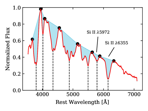
Figure 1: Representative Spextractor function acting on a spectrum of ASASSN-14mf at epoch $\sim 5$ days past maximum $B$ light. The red line indicates the mean function of the corresponding GPR. With a large number of data points, the GPR mean function fits well to the original spectrum, which is still displayed, albeit difficult to discern from the mean. The blue area represents the area integrated in pEW calculations for each line. Note that only the Si II $\lambda 5972$ and $\lambda 6355$ lines are studied in this work, so no special care was taken in extracting other features accurately. The large black dots indicate the points used to linearly determine the pseudo-continuum indicated by the solid blue line.

Figure 1 shows the basic function of the modified Spextractor code on ASASSN-14mf at epoch $\sim 5$ days past maximum light. The red curve is the mean function obtained using GPR and the vertical dashed lines show the position of the flux minima of identified features. We identify the wavelength of the flux minima of the features as the shift due to the (pseudo) photospheric velocities via the non-relativistic Doppler formula. The light blue shading shows the area used to calculate pseudo-equivalent widths (pEWs). Only specified features are marked with Spextractor, and in this work special care is taken only in retrieving accurate measurements for the Si II $\lambda 5972$ and $\lambda 6355$ lines. In order to obtain velocities we assume that the minima identified correspond with the rest wavelengths of Si II $\lambda 5972$ and Si II $\lambda 6355$. We assume a linear continuum approximation between maxima of selected wavelength ranges (as indicated by large black circles in Figure 1) to define features and their pEWs. The $v_{\text{Si II}}$, pEW(Si II $\lambda 5972$), and pEW(Si II $\lambda 6355$) values calculated by Spextractor for each SNe are given in Table 1.

3.2 Cluster Analysis

We invoke a distribution-based cluster analysis using Gaussian mixture models (GMMs) to support grouping objects with related properties (Day, 1969; McLachlan & Peel, 2000). These GMMs are expectation-maximization algorithms that iteratively calculate which input properties maximize the likelihood of a set of $m$-dimensional ($m$-D) Gaussian distributions fitting a given training set of data. After this fit is calculated, a total probability distribution is implicitly given, and so the probability of a point being associated with each of the $n$ distributions can be determined. This method is chosen in order to describe group assignments probabilistically since there appears to be a continuous distribution of multiple group clusters in our sample of data. There is no clear way of separating discrete groups with reasonable confidence — for example, ensuring that each group is distinct for some $3\sigma$ interval. We show that by using Gaussian distributions and, therefore, a well-defined $\sigma$ deviation for each group, the determined groups overlap within $3\sigma$, and so we would consider the groups to be connected or non-discrete. The probability of a SN belonging to any single group may be comparable to that for another group, even though it is within $3\sigma$ of either group’s mean position.

The assumption is also made here that each of the measured quantities $M_{B}$, $v_{\text{Si II}}$, pEW(Si II $\lambda 6355$), and pEW(Si II $\lambda 5972$) can be represented as jointly Gaussian-distributed to first approximation. This approximation is assumed only to have some measure of similarity between these four properties. These quantities are then used as input parameters to the different GMMs calculated and shown in § 4 which in return yield groupings based on the probability of an object being associated with each group. The groupings from any GMM therefore describe similarity between the input quantities from which the GMM was calculated.

For each of our GMMs, the number of clusters (groups), $n$, assigned has been determined first with the assumption that each GMM that includes the two pEW quantities must have at least $n=4$ clusters. Since the original paper of Branch et al. (2006) identified four groups, and it has been customary to break SNe up into the 4 Branch groups, we do not consider clustering data involving pEW(Si II $\lambda 6355$) and pEW(Si II $\lambda 5972$) with fewer than four groups.

In general, the number of clusters used for each GMM may be decided based on standard testing that determines which value of $n$ provides the model that best fits the data. For perfectly Gaussian clusters, $n$ may be determined based on the GMM with the lowest Bayesian Information Criterion (BIC) value (Kass & Raftery, 1995). BIC values of each model presented in this work (see § 4) were calculated for GMMs with $n=1$ to $n=6$. Each one of these calculations are the average of 20 single-trial calculations of the BIC for the model with a given $n$, which is necessary because the GMM algorithm operates with randomized initial conditions, potentially leading to different grouping systems for large values of $n$. Figure 2 (left panel) shows $\Delta(\text{BIC})$ as a function of $n$ for different sets of input parameters, where $\Delta(\text{BIC})$ references the BIC of the $n=1$ GMM such that $\Delta(\text{BIC})=\text{BIC}(n)-\text{BIC}(n=1)$. Therefore, we choose $n$ based on the model yielding the smallest $\Delta(\text{BIC})$. Results from Figure 2 show that all models with pEW(Si II $\lambda 6355$) and pEW(Si II $\lambda 5972$) (”Branch” in the legend, including the 4-D model) prefer a value of $n=2$. However, because it is assumed that $n\geq 4$ for these models, we use $n=4$ for these GMMs.

Figure 2 (right panel) shows the mean Silhouette score $s$ (Rousseeuw, 1987; de Souza et al., 2017) of the different GMMs for $n=2$ to $n=6$. The values of $s$ were calculated using $k$-means clustering (MacQueen, 1967). While the Silhouette score is a good measure of how well the data is separable into clusters, we are guided by the $\Delta(\text{BIC})$ in determining which value of $n$ to use for each model. This is because we establish clusters in this sample based on GMMs and not $k$-means clustering. It is, however, interesting that the Silhouette score consistently favors $n=4$ ($s$ closer to 1 is more preferable) for any model involving both pEW(Si II $\lambda 6355$) and pEW(Si II $\lambda 5972$).

Neither of these measurements is perfect, and that likely indicates that the description of maximum-light properties of SNe using Gaussian distributions is not ideal. However, the Gaussian mixture method’s parametric nature, which allows for a maximum likelihood approach, recommends itself over other, non-parametric methods. In particular, it provides stable probabilistic results, which can be interpreted using standard methods (de Souza et al., 2017).

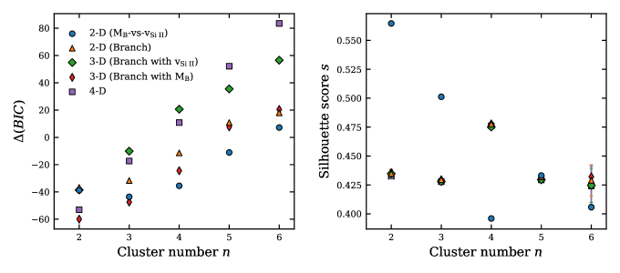
Figure 2: Left panel: $\Delta(\text{BIC})$ versus the cluster number $n$ for each GMM presented in this work. $\Delta(\text{BIC})$ is referenced to the BIC of the $n=1$ GMM. For all dimensionalities except the [$M_{B}$, $v_{\text{Si II}}$ ] input set, models with $n<4$ are not used, in order to follow historical precedent (Branch et al., 2006). Within these restrictions, we find the $n=4$ case to have the smallest $\Delta(\text{BIC})$, thus, these GMMs with $n=4$ are used for this study (see §§ 4.1–4.2). For the [$M_{B}$, $v_{\text{Si II}}$ ] GMM, the $n=3$ model has the smallest $\Delta(\text{BIC})$ value and is therefore used to define $M_{B}$-vs-$v_{\text{Si II}}$ groups discussed in § 4.3. Right panel: the Silhouette score is displayed for each model having $n=2$ to $n=6$ clusters. See text for further description. The plot symbols and colors are shared between panels.

The dimensionality, $m$, of each GMM is determined by the number of SN properties included in training the GMM, which is independent of the number of GMM components $n$. We do not weight any points in the GMMs based on their uncertainty in any quantity.

4 Results

4.1 Branch Clustering

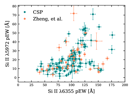
Figure 3: The Branch diagram that includes both the Zheng et al. (2018) and the CSP I+II samples. We see the expected Branch diagram trend with nine extended cool objects with pEW(Si II $\lambda 5972$) $\geq$ 50 Å. Overall, pEW(Si II $\lambda 6355$) in this sample exhibits a mean uncertainty of $\pm$ 4.35 Å and pEW(Si II $\lambda 5972$) exhibits that of $\pm$ 3.02 Å.

Figure 3 shows the Branch diagram obtained for the CSP I+II and Zheng et al. (2018) samples. With this large sample of data, it appears that there are no completely disconnected groupings: a similar and expected result compared to Branch et al. (2006). We do see the expected 0 Å $\leq$ pEW(Si II $\lambda 6355$) $\leq$ 200 Å range. However, although the majority of the objects fall in the expected 0 Å $\leq$ pEW(Si II $\lambda 5972$) $\leq$ 50 Å range, we find a few extended cools with pEW(Si II $\lambda 5972$) $\geq$ 50 Å. Due to the lack of a discrete clustering found between these groups, we perform cluster analysis statistically. Using this entire data set, we create a 2-D GMM in [pEW(Si II $\lambda 5972$), pEW(Si II $\lambda 6355$)] space with (maximal) $n=4$ components, as it is seen from Figure 2 that $n=4$ minimizes $\Delta(\text{BIC})$ for $n\geq 4$. For this and every other GMM that includes pEW(Si II $\lambda 5972$) and pEW(Si II $\lambda 6355$) in its input parameter space, this is also the case. The right panel of Figure 2 shows that the Silhouette score is maximized for these models at $n=4$ and thus supports this number of clusters for this sample. This GMM is displayed in Figure 6. Different colors indicate group membership as a probability distribution of each point belonging to a given group, and different symbols indicate the group corresponding to highest likelihood of membership. Contours correspond to 1-, 2-, and $3\sigma$ from the mean of each group determined by the GMM and is a representation of the covariance of the GMM groups. This figure clearly identifies four groups that indeed correspond to the originally identified Branch groups: core-normals (CN), shallow-silicons (SS), cools (CL), and broad-lines (BL). Note that, in this and future figures with contours representing group membership, we choose to exclude error bars for visual purposes, as the same errors are always displayed in previous figures.

4.2 Higher-Dimensional GMM Clustering

Although the robustness of the Branch groups is seen with a simple 2-D GMM, in intermediate areas between these groups many objects have comparable probabilities of membership to more than one group. For this reason, to achieve more certainty in membership to any single Branch group, we include additional input property that are related to the two pEW parameters in the 2-D GMM. This is expected to provide further constraints for our sample and possibly provide insight into the Branch groups’ relationship with the $M_{B}$-vs-$v_{\text{Si II}}$ diagram, which is discussed in § 4.3.

4.2.1 Inclusion of $v_{\text{Si II}}$

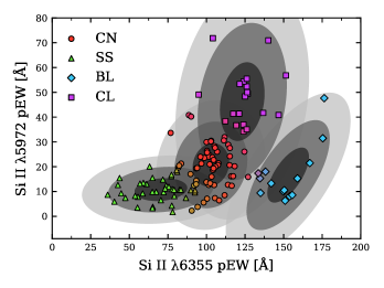
Figure 4: The Branch diagram colored with the [pEW(Si II $\lambda 5972$), pEW(Si II $\lambda 6355$)] GMM ($n=4$ components). Contours indicate 1-, 2-, and $3\sigma$ from the mean of each group determined by the GMM. Different colors indicate group membership as a probability distribution of each point belonging to a given group, and different symbols indicate the group corresponding to highest likelihood of membership.

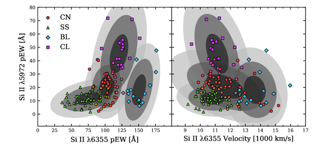
Figure 5: A 3-D GMM analysis of [$v_{\text{Si II}}$, pEW(Si II $\lambda 5972$), pEW(Si II $\lambda 6355$)] ($n=4$ components). The colors in each panel represent group membership and are shared between panels.

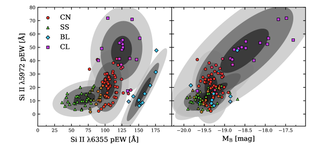
Figure 6: A 3-D GMM analysis of [$M_{B}$, pEW(Si II $\lambda 5972$), pEW(Si II $\lambda 6355$)] ($n=4$ components).

We first look at a 3-D GMM in [$v_{\text{Si II}}$, pEW(Si II $\lambda 5972$), pEW(Si II $\lambda 6355$)] with $n=4$ components (see Figure 2). Figure 6 shows the entire scope of this model. The 2-D contours in each panel are associated with the covariance of every determined group distribution for the respective 2-D slice. The left panel is again a Branch diagram of the sample, and it again clearly separates the sample into Branch-like groups.

It appears that the inclusion of $v_{\text{Si II}}$ information mostly alters the membership likelihoods in intermediate areas surrounding the CN group. This leads to changes in the covariances shown by the contours in Figure 6 as well as the general probability distribution (coloring). Comparing with those from the 2-D model in Figure 6, we find that the $3\sigma$ contour area of the CN group decreased by 13.9%, that of the BL group decreased by 1.8%, and of the CL group decreased by 18.1%, however the $3\sigma$ contour area of the SS group increased by 8.5%.

An important difference is that in areas between groups there is a steeper probability gradient in the 3-D model than the 2-D model in pEW space. More specifically, we refer to this probability gradient as the gradient at a given point of the group membership probability distribution projected into the 2-D subspace, which in this case is the pEW space. Qualitatively, this effect would narrow the shape or size of a group’s contours, which corresponds to the aforementioned decreases in the $3\sigma$ areas of the CN, BL, and CL groups. In intermediate areas between groups it more concretely defines the group membership of many objects that previously showed a nearly equal tendency toward two or more groups. This behavior is expected since naively one would expect a correlation between the pseudo-equivalent width and velocity of the Si II $\lambda 6355$ line, even though they are independently measured.

It is therefore seen that using a GMM to measure the similarity between the two quantities enforces a constraint that quantitatively defines groups. Most noticeably the contours for the CN and CL groups have reduced in size, meaning there is a narrower region in pEW space in which CNs are expected to lie. This illustrates that including the additional $v_{\text{Si II}}$ parameter in the GMM more sharply defines Branch group membership and leads to more certainty in assignment compared to a GMM based on only pEW information.

4.2.2 Inclusion of $M_{B}$

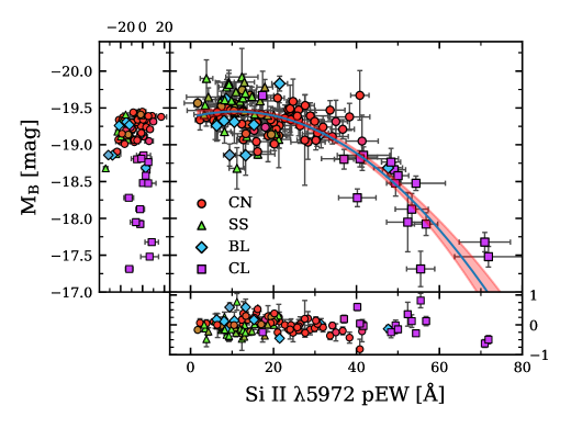
Figure 7: A quadratic fit of the $M_{B}$ versus pEW(Si II $\lambda 5972$) relation colored with the grouping from the 3-D GMM displayed by Figure 6. Residuals are given in panels to the left and below. The light red shaded region represents the uncertainty in the polynomial coefficients themselves. We find the quadratic fit coefficients (from highest to lowest order) to be $a=(6.623\pm 1.168)\times 10^{-4}$, $b=(-1.425\pm 0.657)\times 10^{-2}$, and $c=-19.37\pm 0.07$.

We also investigate the 3-D GMM in [$M_{B}$, pEW(Si II $\lambda 5972$), pEW(Si II $\lambda 6355$)] with $n=4$ components (see Figure 2). Figure 6 again shows the different slices of this model. In the left panel, we again find that the Branch diagram shown has more concretely defined Branch groups than in the 2-D pEW space alone. Again comparing with the contours in the 2-D model displayed in Figure 6, we find that all $3\sigma$ contour areas decrease in size: CN (7.8%), SS (10.3%), BL (59.2%), and CL (23.3%). Clearly BL membership alters more drastically when $M_{B}$ information is included in the GMM. The contours of the BLs are much narrower, so membership is generally contained in a narrower region in pEW space. In fact, with the inclusion of $M_{B}$ the BL group becomes an almost completely distinguishable group, indicating that there may in fact be something distinct about the progenitor system or explosion mechanism that produces BLs.

It is clear from this GMM that using a Gaussian distribution in this cluster analysis is not a perfect method in predicting cluster membership. We begin to see some unexpected behavior in the GMM membership determination. For example, LSQ13aiz (at pEW(Si II $\lambda 6355$) $\approx 133$ and pEW(Si II $\lambda 5972$) $\approx 17$) does indeed appear too bright to be a cool object as is suggested by the GMM. We see, then, that variations in one of the input properties can lead to outlier behavior. As will be seen in § 4.2.3, this problem is partially solved with the inclusion of additional information.

The right panel also shows a strong functional relation between $M_{B}$ and pEW(Si II $\lambda 5972$). We fit a quadratic to this relation, and this is shown in Figure 7. It is interesting that this correlation, along with the Branch group classification, provides a rough $M_{B}$ approximation that is purely based on spectroscopic information. Others have previously noted that pEW(Si II $\lambda 5972$) and $\Delta m_{15}$ are correlated (Hachinger et al., 2008; Folatelli et al., 2013), and we find that this effect is quite robust. Given the relationship between $M_{B}$ and $\Delta m_{15}(B)$, this correlation is essentially a spectroscopic variant of the Phillips relation.

4.2.3 Inclusion of Both $v_{\text{Si II}}$ and $M_{B}$

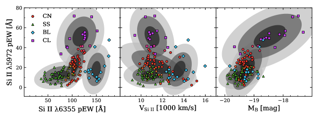
Figure 8: The Branch diagram (left) of the 4-D GMM analysis ($n=4$ components) of all four parameters, showing the robustness of the Branch grouping system. The pEW(Si II $\lambda 5972$)-versus-$v_{\text{Si II}}$ (middle) and pEW(Si II $\lambda 5972$)-versus-$M_{B}$ (right) projections are shown and are color-coded by the same 4-D GMM group membership probabilities. The contours indicate 1-, 2-, and $3\sigma$ of group membership projected into each respective space. We see the groups have become much more constrained and display much overlap that could not be extracted solely with pEW information.

Because we see a strong correlation in [$M_{B}$, pEW(Si II $\lambda 5972$)], we attempt to constrain the Branch groups further by creating a 4-D GMM in [$M_{B}$, $v_{\text{Si II}}$, pEW(Si II $\lambda 5972$), pEW(Si II $\lambda 6355$)] with $n=4$ components (see Figure 2). We show this Branch diagram in the left panel of Figure 8, which again is colored by this 4-D GMM. This GMM indeed still produces the four Branch groups. Even with all four dimensions there is still significant overlap between the CN and SS objects.

The inclusion of both $M_{B}$ and $v_{\text{Si II}}$ constrains the groups further by similarly reducing the size of most contours associated with projected covariance, giving a more concrete assignment to more objects. This overall inclusion decreases the $3\sigma$ contour areas of the CN group (45.6%), the BL group (28.9%), and the CL group (28.7%). However, the $3\sigma$ contour area of the SS group is relatively unchanged, increasing by only 0.6%. In the projection shown, there is more overlap between groups than either 3-D model, which shows that, for our sample, $M_{B}$ and $v_{\text{Si II}}$ contain independent information. That is to say, after including either quantity, including the fourth quantity will constrain the groups further.

Again we see that there are some objects that exhibit relatively substantial dispersion in one or more parameters that appear as outliers. For example, in the middle panel of Figure 8, SN 2008O (with $v_{\text{Si II}}$ $\sim 14.4$ and pEW(Si II $\lambda 5972$) $\sim 47.6$) and SN 2003gn (with $v_{\text{Si II}}$ $\sim 13.2$ and pEW(Si II $\lambda 5972$) $\sim 40.8$) seem most similar to the CL group, however they are deemed BL objects due to their pEW(Si II $\lambda 6355$) and $v_{\text{Si II}}$ values.

Compared to the [pEW(Si II $\lambda 5972$), pEW(Si II $\lambda 6355$)] GMM defined in Figure 6, the inclusion of $M_{B}$ and $v_{\text{Si II}}$ in the GMM allows us to constrain group membership in a way that is not apparent with only pEW(Si II $\lambda 5972$) and pEW(Si II $\lambda 6355$). That is to say, $M_{B}$ and $v_{\text{Si II}}$ may be used to more concretely define Branch groups (remembering that we have a completely different definition for membership that was used by Branch et al., 2006), between which there would otherwise be more uncertainty and continuity in the probability distribution in pEW space.

4.3 $M_{B}$-vs-$v_{\text{Si II}}$ Clustering

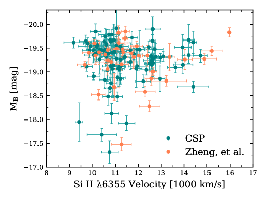
Figure 9: $M_{B}$-vs-$v_{\text{Si II}}$ diagram of both Zheng et al. (2018) and CSP I+II samples. As the CSP sample is included, there are no longer two distinct groups, but rather a continuity of a similar form to the original $M_{B}$-vs-$v_{\text{Si II}}$ diagram. For this sample we find $M_{B}$ to have a mean uncertainty of $\pm$ 0.169 mag and $v_{\text{Si II}}$ to have that of $\pm$ 290 km s^-1.

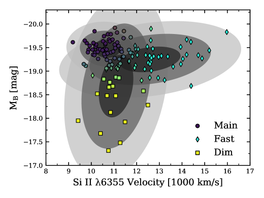
Figure 10: The $M_{B}$-vs-$v_{\text{Si II}}$ diagram colored by a 2-D GMM in [$M_{B}$, $v_{\text{Si II}}$ ] ($n=3$ components) which separates the sample into what we label as the Main, Dim, and Fast groups. The contours correspond to covariance of group membership up to $3\sigma$.

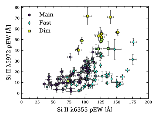
Figure 11: The Branch diagram with groups defined by the 2-D GMM displayed in Figure 10. We see that there is generally no absolute match between the original Polin et al. (2019) groups and the Branch groups as we see many Fast objects contained in BLs as well as CNs and SSs.

Our version of the $M_{B}$-vs-$v_{\text{Si II}}$ diagram with both Zheng et al. (2018) and CSP I+II samples is shown in Figure 9. The general structure of the original plot remains, although the CSP sample extends and fills in the low- to mid-velocity and dim portions of the plot. We see that the added continuity removes the original notion of a clear dichotomy between likely Chandrasekhar mass explosions and sub-Chandrasekhar mass helium detonations (Polin et al., 2019). We use a 2-D GMM in [$M_{B}$, $v_{\text{Si II}}$ ] to account for this and to describe the $M_{B}$-vs-$v_{\text{Si II}}$ group analysis statistically.

Figure 10 shows the $M_{B}$-vs-$v_{\text{Si II}}$ diagram with this GMM with $n=3$ components. This value of $n=3$ minimizes $\Delta(\text{BIC})$ (see Figure 2). While the Silhouette score favors two groups for the $M_{B}$-vs-$v_{\text{Si II}}$ space, we choose this number based on $\Delta(\text{BIC})$, which was calculated using a GMM instead of $k$-means clustering. Again, the lack of a strong preference is likely an indication of the inadequacy of the description of the groups with Gaussian distributions. We refer to these three determined groups as the $M_{B}$-vs-$v_{\text{Si II}}$ groups — namely the Main group, the Dim group, and the Fast group.

The Main $M_{B}$-vs-$v_{\text{Si II}}$ group seems to resemble very closely the more populous group of SNe in the original $M_{B}$-vs-$v_{\text{Si II}}$ diagram that Polin et al. (2019) interpreted as near-Chandrasekhar-mass explosions. Conversely, the Dim and Fast groups together make-up the entirety of objects that Polin et al. (2019) identified with sub-Chandrasekhar models produced with a thin helium shell.

One may naively expect the Main group to have good overlap with the CN Branch group, the Fast group to overlap with the BLs [as with high $v_{\text{Si II}}$ one would expect large pEW(Si II $\lambda 6355$)], and the Dim group to overlap with the CLs. Figure 11 shows the Branch diagram colored with the $M_{B}$-vs-$v_{\text{Si II}}$ groups defined by the GMM illustrated in Figure 10. Comparing with our 4-D GMM description of the Branch groups in Figure 8, it is clear that there is not a good match between the $M_{B}$-vs-$v_{\text{Si II}}$ groups defined by [$M_{B}$, $v_{\text{Si II}}$ ] and the Branch groups. The Main group is made up mostly of both CN and SS SNe. However, we also see many Fast group objects are either CNs or SSs. This is actually quite surprising, since a priori one would expect a strict relationship between the high-velocity $M_{B}$-vs-$v_{\text{Si II}}$ group and the BLs. We see, then, that there is much dispersion in the relationship between $v_{\text{Si II}}$ and pEW(Si II $\lambda 6355$). The inconsistency here must be that the intermediate area between the Main and Fast groups cannot be established exclusively in [$M_{B}$, $v_{\text{Si II}}$ ]. Finally, we remark that the Dim group tends to associate with the CLs nearly entirely, which is expected.

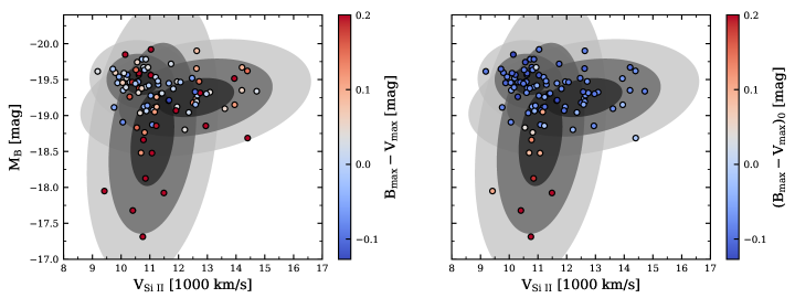
Figure 12: $M_{B}$-vs-$v_{\text{Si II}}$ diagram of the CSP I+II samples (without the Zheng et al. (2018) sample, as they did not provide colors for their sample). The left panel is coded for $B_{\text{max}}-V_{\text{max}}$ color that is uncorrected for host galaxy extinction, whereas the right panel is coded for $(B_{\text{max}}-V_{\text{max}})_{0}$ color that is corrected for host extinction. The color scale is truncated for $(B_{\text{max}}-V_{\text{max}})_{0}$ $>0.2~{}\text{mag}$ due to relatively large separation of 19 outliers with $0.2~{}\text{mag}<B_{\text{max}}-V_{\text{max}}\leq 0.939~{}\text{mag}$ (left panel) and four outliers with $0.2~{}\text{mag}<$ $(B_{\text{max}}-V_{\text{max}})_{0}$ $\leq 0.536$ mag (right panel). The contours are exactly those from Figure 10, which indicate the [$M_{B}$, $v_{\text{Si II}}$ ] GMM covariance. $M_{B}$ plotted in both panels is the same, always including host extinction.

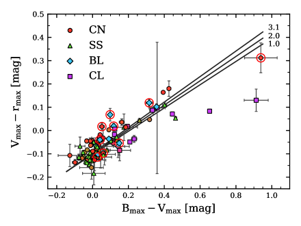
Figure 13: Color-color figure of MW extinction-corrected $V_{\text{max}}-r_{\text{max}}$ versus $B_{\text{max}}-V_{\text{max}}$ for the CSP I+II subsample. The figure is colored by 4-D Branch group membership, and red circles indicate objects with $v_{\text{Si II}}$ $>$ 13,000 km s^-1. $R_{V}$ values of 1.0, 2.0, and 3.1 are indicated. The $R_{V}$ lines show the general direction of displacement due to a correction for reddening. In general, non-CL SNe are generally insensitive to the value of $R_{V}$ and follow a trajectory expected from a dust reddening law. These Fast group SNe also follow the dust trajectory, suggesting that for some reason they tend to be relatively highly extinguished in their host galaxies. While this does not prove that they have the correct $M_{B}$ determined by SNooPy, it makes it plausible.

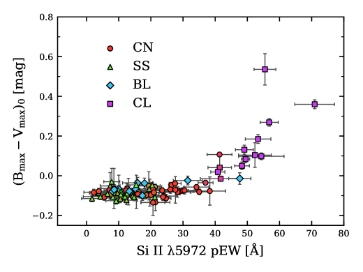
Figure 14: $(B_{\text{max}}-V_{\text{max}})_{0}$ versus pEW(Si II $\lambda 5972$) of the CSP I+II samples with 4-D Branch groups colored. We find that at pEW(Si II $\lambda 5972$) $\lesssim$ 40 Å, there is no correlation between the two quantities, which is expected by the $M_{B}$ versus pEW(Si II $\lambda 5972$) relation we find in § 4.2.2.

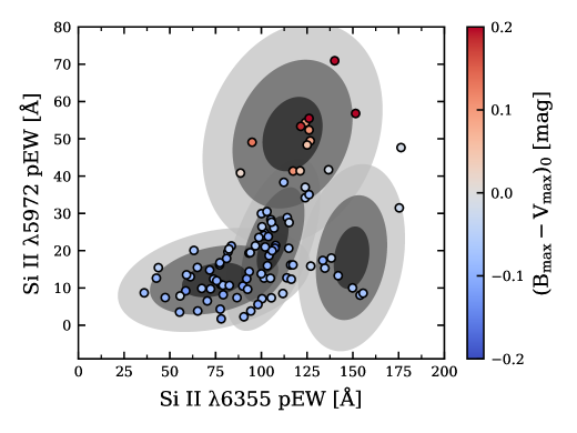
Figure 15: Branch diagram of the CSP I+II samples coded for $(B_{\text{max}}-V_{\text{max}})_{0}$ color. The color scale is truncated for $(B_{\text{max}}-V_{\text{max}})_{0}$ $>0.2$ in the same way as Figure 12. The contours are exactly those from Figure 8, indicating our defined 4-D Branch groups.

In Figure 12 we show $M_{B}$-vs-$v_{\text{Si II}}$ diagrams for CSP I+II data, excluding the Zheng et al. (2018) sample, as colors were not provided for this sample. The left panel is coded for $B_{\text{max}}-V_{\text{max}}$ color that is uncorrected for host galaxy extinction, and the right panel is coded for $(B_{\text{max}}-V_{\text{max}})_{0}$ which is corrected for host extinction (Burns et al., 2018). Both colors are corrected for MW extinction. Contours in this figure are identical to those found in the [$M_{B}$, $v_{\text{Si II}}$ ] GMM from Figure 10. From the left panel we see the similar result from Polin et al. (2019) that the bluest objects are consistently found within the Main group. However, comparing the two, we see that, after correcting for both MW and host extinction, $(B_{\text{max}}-V_{\text{max}})_{0}$ only seems to have a dependence on $M_{B}$. We find no evidence of red objects which are intrinsically bright. It is evident that both the Main and Fast groups primarily contain intrinsically bluer objects than the Dim group. After correcting for host extinction, the group that was claimed to follow sub-Chandrasekhar-mass models by Polin et al. (2019) does not display a more consistent redder color than the more populated clump of Main group objects, indicating that these high velocity objects are not likely to come from sub-Chandrasekhar-mass explosions.

4.3.1 Color of the Fast Group SNe

Table 2: Subset of Fast CSP I+II SNe with $v_{\text{Si II}}$ $>$ 13,000 km s^-1.

SN	$(B_{\text{max}}-V_{\text{max}})_{0}$	$A_{V}^{\text{MW}}$	$A_{V}^{\text{Host}}$
	(mag)	(mag)	(mag)
ASASSN-14hr	$-0.074\pm 0.018$	0.04	0.31
CSP15B	$-0.024\pm 0.022$	0.20	0.36
LSQ13aiz	$-0.100\pm 0.024$	0.24	0.39
PTF13duj	$-0.073\pm 0.024$	0.21	0.15
2006br	$-0.064\pm 0.101$	0.06	2.28
2008go	$-0.078\pm 0.016$	0.10	0.09
2008O	$-0.014\pm 0.029$	0.24	0.37
2009Y	$-0.070\pm 0.025$	0.27	0.28
2012bl	$-0.085\pm 0.017$	0.09	0.01

It is seen from Figure 12 that nine Fast objects (chosen by $v_{\text{Si II}}$ $>$ 13,000 km s^-1) from the CSP I+II sample generally exhibit a redder $B_{\text{max}}-V_{\text{max}}$ color (when not corrected for host galaxy extinction). These SNe are listed in Table 2, along with their $(B_{\text{max}}-V_{\text{max}})_{0}$ color and extinction values for Milky Way and host galaxies. This is in line with the results from Polin et al. (2019) who showed a similar plot to the left panel of Figure 12. Note that Polin et al. (2019) do not correct for host galaxy extinction. Comparing the two panels of Figure 12 suggests, then, that these Fast objects seem to be quite reddened in their host galaxy. Figure 13 shows that in [$V_{\text{max}}-r_{\text{max}}$, $B_{\text{max}}-V_{\text{max}}$] space, non-CL SNe generally follow a line that is relatively insensitive to the value of $R_{V}$, giving confidence that these Fast SNe are for some reason preferentially reddened in their host galaxies and that the inferred host extinction is not due to some underlying assumption in the SNooPy templates that is misinterpreted. Since Zheng et al. (2018) used MLCSk2 and a fixed $R_{V}$ to infer host extinction and $M_{B}$, although similar but not identical to the methods of SNooPy, it lends some credence to the argument that SNooPy is not somehow mis-correcting the Fast subsample. However, we have introduced a correlation between pEW(Si II $\lambda 5972$) and $M_{B}$ as well as pEW(Si II $\lambda 5972$) and $(B_{\text{max}}-V_{\text{max}})_{0}$ just by using SNooPy to fit for these quantities. The same would be true if we were to use MLCS2k2 or SALT, because their light-curve shape parameters would also be highly correlated with pEW(Si II $\lambda 5972$). Nonetheless while these objects have distinct spectroscopic properties, we are assuming they all follow the same intrinsic color–$s_{BV}$ relation from Burns et al. (2014) in order to perform the extinction corrections.

Wang et al. (2009) noted this importance of $v_{\text{Si II}}$, splitting SNe into two groups and noting that the group with $v_{\text{Si II}}$ $\gtrsim$ 11,800 km s^–1 preferred a lower value of $R_{V}\sim 1.6$. Figure 13 shows that these Fast SNe follow a dust trajectory which is insensitive to $R_{V}$, which is an indication that the trend seen in Figure 12 is likely due to extinction from dust in the host. This preference for these Fast objects to appear in dusty regions (perhaps near the core, see Uddin et al., 2020) should be the subject of future work.

We also note that in contrast to the $B_{\text{max}}-V_{\text{max}}$ values presented in Polin et al. (2019), when corrected for host extinction the $(B_{\text{max}}-V_{\text{max}})_{0}$ range is much narrower, mostly falling within $-0.2<$ $(B_{\text{max}}-V_{\text{max}})_{0}$ $<0.2$, having only four outliers with $(B_{\text{max}}-V_{\text{max}})_{0}$ $>0.2$ (shown more explicitly in Figure 14). Figure 14 shows $(B_{\text{max}}-V_{\text{max}})_{0}$ versus pEW(Si II $\lambda 5972$) for the CSP I+II sample. We see that at low pEW(Si II $\lambda 5972$) there is no correlation between the two quantities. This is expected from Figure 12, because only Dim objects have a large increase in $(B_{\text{max}}-V_{\text{max}})_{0}$ compared to brighter objects from the Main and Fast groups that exhibit bluer color with no other noticeable trend. Generally there is only a spread of about 0.15 magnitude in $(B_{\text{max}}-V_{\text{max}})_{0}$ for most SNe Ia.

We also include a Branch diagram colored in $(B_{\text{max}}-V_{\text{max}})_{0}$ for reference to the Branch groups in Figure 15. Contours in this figure are exactly those determined by the 4-D GMM that are displayed in Figure 8. We see that, as expected, the CLs are generally the reddest objects, where there is no other trend between the other three groups.

5 Discussion

5.1 Constraining the Branch GMM

Supplementing the two quantities pEW(Si II $\lambda 5972$) and pEW(Si II $\lambda 6355$) with more information provides more certainty in Branch group assignment. Quantitatively, the 4-D GMM has been shown to decrease the size of GMM covariance contours by making a constraint that values must also be similar in additional dimensions. When we compare the three different models in § 4.2, however, we see that uncertainty in the [pEW(Si II $\lambda 5972$), pEW(Si II $\lambda 6355$)] GMM mostly decreases with the inclusion of only a single quantity. Therefore, although we take the 4-D GMM as our defining model for Branch groups as it includes additional $M_{B}$ information that we show is non-linearly correlated with pEW(Si II $\lambda 5972$), it can still be approximated with only the inclusion of $v_{\text{Si II}}$. In this way, the Branch groups can be approximated purely with spectroscopic data. The effects obtained above are interesting given works showing that the inclusion of $v_{\text{Si II}}$ reduces the scatter of Hubble residuals (Foley & Kasen, 2011) and that there appears to be a correlation in the sign of the Hubble residuals and the value of $v_{\text{Si II}}$ (Siebert et al., 2020). Recently, it was suggested that SNe Ia with high $v_{\text{Si II}}$ are closely associated with massive host environments and that high $v_{\text{Si II}}$ is due to a variation in explosion mechanism (Pan, 2020). We find that the BL group is more likely to be distinct, but it would be good to identify the environments of objects in different Branch groups. We do note that the tendency of the Fast objects to be strongly extinguished in their hosts is likely an indication about the nature of the environment of these SNe Ia.

It is also seen in Figure 8 that 26 SNe change their most probable group assignment between the 2-D GMM, the 3-D GMM with $v_{\text{Si II}}$ inclusion, and the 4-D GMM. Table 3 details the changes involved for this sample. Out of the total 26 SNe, 24 are reassigned with the inclusion of both $M_{B}$ and $v_{\text{Si II}}$ to the GMM, which is substantial compared to the total sample size of 133 SNe. We find that including these two parameters has the greatest effect on CN and CL objects, with little to no effect on SS and BL objects that are defined in the 2-D model. This may be due to the relationship we find between $M_{B}$ and pEW(Si II $\lambda 5972$) coupled with a dispersion in the $v_{\text{Si II}}$–pEW(Si II $\lambda 6355$) relation, however more work must be done to determine the dominant quantities that govern the changes between each group. Ultimately, group assignment and any physical attributes that objects of each group may possess are not solely a function of pseudo-equivalent widths, but of also their other properties such as $M_{B}$ and $v_{\text{Si II}}$, as is shown in this work. Interestingly, the classification changes from CN to SS are fairly stable going from the 3-D GMM to the 4-D GMM, and also the identification of BL is stable from 3-D to 4-D. The most noticeable difference from 3-D to 4-D is CL $\to$ CN for a half-dozen supernovae.

Table 3: SNe with Branch group membership changes between the 2-D GMM, the spectroscopic 3-D GMM with $v_{\text{Si II}}$ dependence, and the 4-D GMM. The group for each model is based on the most probable assignment determined by each GMM.

SN	2-D	3-D ($v_{\text{Si II}}$)	4-D
	Group	Group	Group
CSP14acl	CN	CN	SS
LSQ13ry	CN	CN	SS
2005el	CN	CN	SS
2004ey	CN	SS	CN
2008fr	CN	SS	CN
ASASSN-15al	CN	SS	SS
ASASSN-15hf	CN	SS	SS
2000dn	CN	SS	SS
2005bg	CN	SS	SS
2005cf	CN	SS	SS
2005hc	CN	SS	SS
2006le	CN	SS	SS
2008bq	CN	SS	SS
2013fy	CN	SS	SS
2008hu	CN	BL	BL
2002dl	CN	CN	CL
2003gt	CN	CN	CL
2011iv	CN	CN	CL
ASASSN-14hu	SS	CN	CN
2003gn	CL	BL	BL
PS1-14ra	CL	CL	CN
PTF14w	CL	CL	CN
2007on	CL	CL	CN
2008ec	CL	CL	CN
2008fl	CL	CL	CN
2011jh	CL	CL	CN

5.2 $M_{B}$-vs-$v_{\text{Si II}}$ Groups

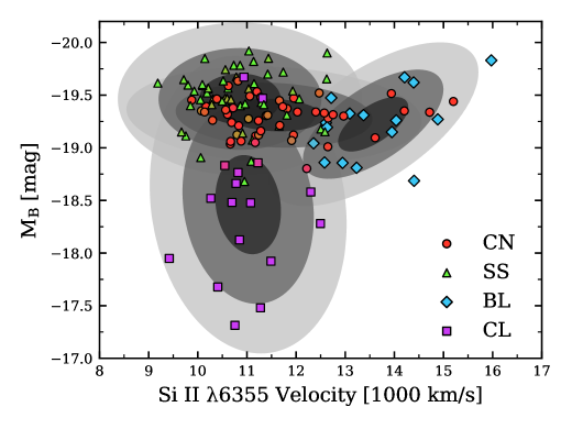
Figure 16: The $M_{B}$-vs-$v_{\text{Si II}}$ diagram of the 4-D GMM analysis from § 4.2.3. The contours indicate covariance (up to $3\sigma$) of group membership projected into [$M_{B}$, $v_{\text{Si II}}$ ] space. We see that the Main group consists of both CN and SS objects and that the Fast group is separated into both BL and CN objects. This separation implies there is a dispersion in the relationship between $v_{\text{Si II}}$ and pEW(Si II $\lambda 6355$). As expected, the Dim group almost exclusively contains CL objects.

Our analysis does not show the clear dichotomy in [$M_{B}$, $v_{\text{Si II}}$ ] space found in Polin et al. (2019) when we include the CSP I+II samples in addition to the Zheng et al. (2018) sample. In particular, their result seems to be due to not correcting for reddening in the host, when plotting $(B_{\text{max}}-V_{\text{max}})_{0}$. The only intrinsically red objects are the Dims/CLs. When all four parameters are accounted for in the GMM, as shown in Figure 16, we see that the Main group consists primarily of CN and SS objects, the Fast group is dominated by BL objects with only a few CN objects, and the Dim group is again made up primarily of CL objects. The Fast objects can indeed be divided using their pEW properties. Therefore, the Fast group SNe do not need to stem from sub-Chandrasekhar explosions, and additional information is required to more concretely determine the underlying physics involved.

If we assume the Main group to be the union of both SS and CN objects, we do find that, in comparing Figure 10 with the modified $M_{B}$-vs-$v_{\text{Si II}}$ diagram presented in Figure 16, the projected covariances into [$M_{B}$, $v_{\text{Si II}}$ ] space show significant qualitative change. The BL contours that are associated with the Fast group are noticeably smaller, meaning it is a more well-constrained grouping with less uncertainty between the BLs and other groups. The Main group contains both CN and SS objects so it is important to determine if there are other distinctions between CN and SS objects that can be related to variations in the progenitors or explosion mechanisms.

From Figure 12 we see that the 4-D grouping system projected onto [$M_{B}$, $v_{\text{Si II}}$ ] space does not sort SNe by $(B_{\text{max}}-V_{\text{max}})_{0}$ color. We find that $(B_{\text{max}}-V_{\text{max}})_{0}$ is mostly distinct only for Dims, and the Fast group color is bluer than Dims, regardless of whether the object is a CN or BL SN. More work must be done to further sub-classify these SNe Ia.

5.3 Branch Group Relation with $s_{BV}$

Figure 17: Illustration of the Phillips relation as $M_{B}$ versus $s_{BV}$. Points are color-coded by the 4-D Branch groups (left panel) and the $M_{B}$-vs-$v_{\text{Si II}}$ groups (right panel).

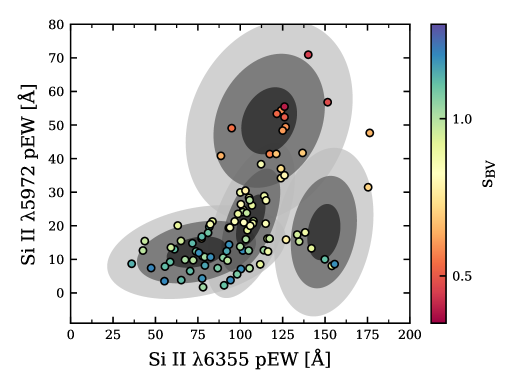
Figure 18: Branch diagram of the CSP I+II samples coded for color stretch parameter $s_{BV}$. The contours are exactly those from Figure 8, indicating our defined 4-D Branch groups.

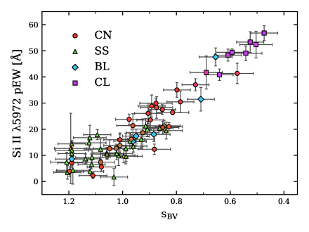
Figure 19: pEW(Si II $\lambda 5972$) versus $s_{BV}$ of the CSP I+II samples colored by the 4-D Branch groups. We see a linear trend for SNe with $s_{BV}\lesssim 1.0$.

Figure 17 shows the Phillips/Burns relation color-coded by Branch group (left panel) and by $M_{B}$-vs-$v_{\text{Si II}}$ group (right panel). Both the CL and Dims are intrinsically dim, and there is much overlap between them, as seen in § 5.2. The Branch diagram coded for $s_{BV}$ is displayed in Figure 18 and it shows that $s_{BV}$ does not distinguish between CN and BL SNe with high values of $v_{\text{Si II}}$ as is seen in Figure 16. It will be interesting to understand what causes this variation to better improve the use of SNe Ia as cosmological probes.

In Figure 17 there appears to be a transition region of SS into CN that corresponds to a transition of the Main group into the Fast group. It could be that there is some underlying parameterization involved that better explains the dispersion in this Phillips/Burns relation, such as a dependency upon $M_{B}$-vs-$v_{\text{Si II}}$ group membership or $v_{\text{Si II}}$. This interesting behavior is left to be studied in future work.

Figure 19 shows that a Phillips-like relation exists for pEW(Si II $\lambda 5972$) and the color stretch parameter, $s_{BV}$ (Burns et al., 2018). In other words, pEW(Si II $\lambda 5972$) acts as a stand-in for $M_{B}$ (see s 6 and 7). Figure 19 also shows the 4-D Branch group placement for this relation. At high $s_{BV}$ ($s_{BV}\gtrsim 1.0$), little correlation is found between pEW(Si II $\lambda 5972$) and $s_{BV}$, which is expected because the dependency of $s_{BV}$ on $M_{B}$ decreases for brighter SNe (seen in Figure 17). However, a linear trend is found for $s_{BV}\lesssim 1.0$.

6 Conclusions

We have shown that a 4-D Gaussian mixture model (GMM) analysis of [$M_{B}$, $v_{\text{Si II}}$, pEW(Si II $\lambda 5972$), pEW(Si II $\lambda 6355$)] with $n=4$ components yields robust groupings that strongly identify the four Branch groups: core-normals (CN), shallow-silicons (SS), broad-lines (BL), and cools (CL). We have shown that there seems to be a strong correlation between $M_{B}$ and pEW(Si II $\lambda 5972$), and because of this we suggest that the quantities pEW(Si II $\lambda 6355$), pEW(Si II $\lambda 5972$), and $v_{\text{Si II}}$ can be used to approximate this 4-D model with only spectroscopic quantities. Furthermore, the 3-D GMM makes the BL group nearly distinct; it seems reasonable that this subclass of SNe would be distinct from the rest of the SNe Ia as suggested previously by Wang et al. (2013). One possibility is that the high velocity of the photosphere is produced by a shell, such as that produced by a pulsating delayed detonation (Hoeflich et al., 1996; Dessart et al., 2014).

The original $M_{B}$-vs-$v_{\text{Si II}}$ diagram was interpreted to separate SNe Ia into two groups based on $M_{B}$ and $v_{\text{Si II}}$ that likely corresponded to Chandrasekhar-mass explosions and sub-Chandrasekhar explosions (Polin et al., 2019). We find that this is an incomplete description; rather than a clear dichotomy in [$M_{B}$, $v_{\text{Si II}}$ ] space, there are three connected groups. Ultimately we find that SN subtypes are better-delineated by the Branch groups using GMMs. We define these three $M_{B}$-vs-$v_{\text{Si II}}$ groups as: the Main group consisting of CNs and SSs, the Fast group consisting of BLs and a subset of CNs, and the Dim group that consists of CLs. It is shown that Fast objects can be divided using their Branch group membership (Si II pEWs), and this division may aid in predicting their underlying explosion mechanisms. We find that this separation is generally unexplained by the color stretch parameter $s_{BV}$, and so future work must be done to explain this dispersion.

Open access to each of these GMMs is provided at https://github.com/anthonyburrow/SNIaDCA. In future work we plan to use a tool such as principal component analysis to determine just how much pEW(Si II $\lambda 5972$) is captured in $M_{B}$ and how much pEW(Si II $\lambda 6355$) is captured in $v_{\text{Si II}}$ and other covariances including $(B_{\text{max}}-V_{\text{max}})_{0}$ and $s_{BV}$ as well as extinction properties such as color excess $E(B-V)$ and $R_{V}$.

7 Acknowledgments

The work of the CSP-II has been generously supported by the NSF under grants AST-1008543, AST-1613426, AST-1613455, AST-1613472, and in part by a Sapere Aude Level 2 grant funded by the Danish Agency for Science and Technology and Innovation (PI M.S.). AB and EB were supported in part by NASA grant 80NSSC20K0538. L.G. was funded by the European Union’s Horizon 2020 research and innovation programme under the Marie Skłodowska-Curie grant agreement No. 839090. This work has been partially supported by the Spanish grant PGC2018-095317-B-C21 within the European Funds for Regional Development (FEDER). M.S. is supported by generous grants (13261 and 28021) from VILLUM FONDEN, and also by a project grant (8021-00170B) from the Independent Research Fund Denmark. PJB, KK, and NBS gratefully acknowledge the support of the George P. and Cynthia Woods Mitchell Institute for Fundamental Physics and Astronomy. We also thank the Mitchell Foundation for their sponsorship of the Cook’s Branch Workshop on Supernovae where much of this science was discussed.

Appendix A Inclusion of Errors to GP Kernel

In this section we briefly describe most major changes to Spextractor we invoke pertaining to spectrum fitting using Gaussian process regression (GPR) that are used in calculating line velocities and pseudo-equivalent widths. The background information given paraphrases a more detailed explanation provided in Murphy (2012).

A Gaussian process is used to infer a distribution over functions $p(f|\mathbf{X},\mathbf{y})$ given some observed input set $\mathbf{X}$ and output set $\mathbf{y}$ such that $y_{i}=f(x_{i})$ for $y_{i}\in\mathbf{y}$ and $x_{i}\in\mathbf{X}$. In this paper, for fitting spectra with a GPR, $\mathbf{y}$ is the set of flux measurements, and $\mathbf{X}$ is the corresponding wavelengths at which these measurements were taken. The Gaussian process is defined to assume that $p(f(x_{1}),...,f(x_{N}))$ is jointly Gaussian for an arbitrary set of inputs $x_{1},...,x_{N}$ for $N$ observation points in $\mathbf{X}$ and therefore in $\mathbf{y}$. This joint Gaussian distribution has mean $\mathbf{\mu}(\mathbf{x})$ and covariance $\mathbf{K}(\mathbf{x})$ given by $K_{ij}=\kappa(x_{i},x_{j})$, where $\kappa$ is the positive definite kernel function for which we choose the Matérn 3/2 covariance function (Rasmussen & Williams, 2006) as does the original Spextractor code. The functional distribution is then normally distributed as

$$\begin{pmatrix}\mathbf{f}\\ \mathbf{f}*\end{pmatrix}=\mathcal{N}\left(\begin{pmatrix}\mathbf{\mu}\\ \mathbf{\mu}_{*}\end{pmatrix},\begin{pmatrix}\mathbf{K}&\mathbf{K}_{*}\\ \mathbf{K}_{*}^{\mathsf{T}}&\mathbf{K}_{**}\end{pmatrix}\right),$$ (A1)

where $\mathbf{f}_{*}$ are functional outputs of $\mathbf{X}$, and $\mathbf{K}=\kappa(\mathbf{X},\mathbf{X})$, $\mathbf{K}_{*}=\kappa(\mathbf{X},\mathbf{X}_{*})$, and $\mathbf{K}_{**}=\kappa(\mathbf{X}_{*},\mathbf{X}_{*})$, where $\mathbf{X}_{*}$ is some test (or prediction) input set. The output values $\mathbf{f}_{*}$ are then predicted with a GPR as mean values and associated variances for each test point. In this work we modify Spextractor such that $\mathbf{X}_{*}\neq\mathbf{X}$ to allow a representation of the variance between observed data points. More specifically, $\mathbf{X}_{*}$ was selected as a uniform distribution of 2,000 values that spanned the given spectrum.

If there are independently and identically distributed uncertainties $\epsilon_{i}$ (see, for example, Murphy, 2012) in the observed output such that

$$y_{i}=f(x_{i})+\epsilon_{i},$$ (A2)

where in general each $\epsilon_{i}$ may not be equal to one another, we may write the distribution as

$$\begin{pmatrix}\mathbf{\mathbf{y}}\\ \mathbf{f}*\end{pmatrix}=\mathcal{N}\left(\begin{pmatrix}\mathbf{\mu}\\ \mathbf{\mu}_{*}\end{pmatrix},\begin{pmatrix}\mathbf{K}_{y}&\mathbf{K}_{*}\\ \mathbf{K}_{*}^{\mathsf{T}}&\mathbf{K}_{**}\end{pmatrix}\right),$$ (A3)

where $\mathbf{K}_{y}$ is the covariance matrix defined by $\mathbf{K}_{y}\equiv\mathbf{K}+(\sigma^{2})^{\mathsf{T}}I_{N}$ with $\sigma^{2}$ being a vector of associated output uncertainties and $I_{N}$ the $N\times N$ identity. We therefore add flux uncertainties $\sigma_{flux}^{2}$ in quadrature to the kernel when flux uncertainties were provided.

References

- Ashall et al. (2020) Ashall, C., Lu, J., Burns, C., et al. 2020, ApJ, 895, L3
- Bailey et al. (2009) Bailey, S., Aldering, G., Antilogus, P., et al. 2009, A&A, 500, L17
- Benetti et al. (2005) Benetti, S., Cappellaro, E., Mazzali, P. A., et al. 2005, ApJ, 623, 1011
- Bongard et al. (2006) Bongard, S., Baron, E., Smadja, G., Branch, D., & Hauschildt, P. 2006, ApJ, 647, 480
- Branch et al. (2006) Branch, D., Dang, L. C., Hall, N., et al. 2006, PASP, 118, 560
- Burns et al. (2011) Burns, C. R., Stritzinger, M., Phillips, M. M., et al. 2011, AJ, 141, 19
- Burns et al. (2014) —. 2014, ApJ, 789, 32
- Burns et al. (2018) Burns, C. R., Parent, E., Phillips, M. M., et al. 2018, ApJ, 869, 56
- Day (1969) Day, N. E. 1969, Biometrika, 56, 463–474
- de Souza et al. (2017) de Souza, R. S., Dantas, M. L. L., Costa-Duarte, M. V., et al. 2017, MNRAS, 472, 2808
- Dessart et al. (2014) Dessart, L., Blondin, S., Hillier, D. J., & Khokhlov, A. 2014, MNRAS, 441, 532
- Folatelli et al. (2013) Folatelli, G., et al. 2013, ApJ, 773, 53
- Foley & Kasen (2011) Foley, R. J., & Kasen, D. 2011, ApJ, 729, 55
- Goldhaber et al. (2001) Goldhaber, G., et al. 2001, ApJ, 558, 359
- GPy (2012) GPy. 2012, GPy: A Gaussian process framework in python, http://github.com/SheffieldML/GPy, ,
- Guillochon et al. (2017) Guillochon, J., Parrent, J., Kelley, L. Z., & Margutti, R. 2017, ApJ, 835, 64
- Hachinger et al. (2008) Hachinger, S., Mazzali, P. A., Tanaka, M., Hillebrandt, W., & Benetti, S. 2008, MNRAS, 389, 1087
- Hamuy et al. (1996) Hamuy, M., Phillips, M. M., Suntzeff, N. B., et al. 1996, AJ, 112, 2398
- Hoeflich et al. (1996) Hoeflich, P., Khokhlov, A., Wheeler, J. C., et al. 1996, ApJ, 472, L81
- Hsiao et al. (2019) Hsiao, E. Y., Phillips, M. M., Marion, G. H., et al. 2019, PASP, 131, 014002
- Hunter (2007) Hunter, J. D. 2007, Computing in Science & Engineering, 9, 90
- Jha et al. (2007) Jha, S., Riess, A. G., & Kirshner, R. P. 2007, ApJ, 659, 122
- Kass & Raftery (1995) Kass, R., & Raftery, A. 1995, Journal of the American Statistical Association, 90, 773
- Krisciunas et al. (2017) Krisciunas, K., Contreras, C., Burns, C. R., et al. 2017, AJ, 154, 211
- MacQueen (1967) MacQueen, J. B. 1967, in Proc. of the fifth Berkeley Symposium on Mathematical Statistics and Probability, ed. L. M. L. Cam & J. Neyman, Vol. 1 (University of California Press), 281–297
- McLachlan & Peel (2000) McLachlan, G. J., & Peel, D. 2000, Finite mixture models, Wiley series in probability and statistics (New York: J. Wiley & Sons), iSBN 978-0471006268
- Murphy (2012) Murphy, K. 2012, Machine Learning: A Probabilistic Perspective, 1st edn., Adaptive Computation and Machine Learning series (Cambridge, MA: MIT Press)
- Nugent et al. (1995) Nugent, P., Phillips, M., Baron, E., Branch, D., & Hauschildt, P. 1995, ApJ, 455, L147
- Oliphant (2006) Oliphant, T. E. 2006, A guide to NumPy (USA: Trelgol Publishing)
- Pan (2020) Pan, Y.-C. 2020, ApJ, submitted, arXiv:2004.14544
- Papadogiannakis (2019) Papadogiannakis, S. 2019, PhD thesis, Stockholm University, Stockholm, doi:https://tinyurl.com/yc4gyah4
- Pedregosa et al. (2011) Pedregosa, F., Varoquaux, G., Gramfort, A., et al. 2011, Journal of Machine Learning Research, 12, 2825
- Phillips (1993) Phillips, M. M. 1993, ApJ, 413, L105
- Phillips et al. (1999) Phillips, M. M., Lira, P., Suntzeff, N. B., et al. 1999, AJ, 118, 1766
- Phillips et al. (2019) Phillips, M. M., Contreras, C., Hsiao, E. Y., et al. 2019, PASP, 131, 014001
- Polin et al. (2019) Polin, A., Nugent, P., & Kasen, D. 2019, ApJ, 873, 84
- Rasmussen & Williams (2006) Rasmussen, C. E., & Williams, C. K. I. 2006, Gaussian Processes for Machine Learning (Cambridge, MA: MIT Press), doi:http://www.gaussianprocess.org/gpml/
- Riess et al. (1996) Riess, A. G., Press, W. H., & Kirshner, R. P. 1996, ApJ, 473, 88
- Rousseeuw (1987) Rousseeuw, P. J. 1987, Journal of Computational and Applied Mathematics, 20, 53
- Siebert et al. (2020) Siebert, M. R., Foley, R. J., Jones, D. O., & Davis, K. W. 2020, MNRAS, 493, 5713
- Tripp (1998) Tripp, R. 1998, A&A, 331, 815
- Uddin et al. (2020) Uddin, S., et al. 2020, ApJ
- van der Walt et al. (2011) van der Walt, S., Colbert, S. C., & Varoquaux, G. 2011, Computing in Science & Engineering, 13, 22
- Wang et al. (2013) Wang, X., Wang, L., Filippenko, A. V., Zhang, T., & Zhao, X. 2013, Science, 340, 170
- Wang et al. (2009) Wang, X., Filippenko, A. V., Ganeshalingam, M., et al. 2009, ApJ, 699, L139
- Zheng et al. (2018) Zheng, W., Kelly, P. L., & Filippenko, A. V. 2018, ApJ, 858, 104