Mutual information-assisted Adaptive Variational Quantum Eigensolver Ansatz Construction

Abstract

Adaptive construction of ansatz circuits offers a promising route towards applicable variational quantum eigensolvers (VQE) on near-term quantum hardware. Those algorithms aim to build up optimal circuits for a certain problem. Ansatz circuits are adaptively constructed by selecting and adding entanglers from a predefined pool in those algorithms. In this work, we propose a way to construct entangler pools with reduced size for those algorithms by leveraging classical algorithms. Our method uses mutual information (MI) between the qubits in classically approximated ground state to rank and screen the entanglers. The density matrix renormalization group (DMRG) is employed for classical precomputation in this work. We corroborate our method numerically on small molecules. Our numerical experiments show that a reduced entangler pool with a small portion of the original entangler pool can achieve same numerical accuracy. We believe that our method paves a new way for adaptive construction of ansatz circuits for variational quantum algorithms.

I Introduction

Quantum computers promise to provide speed-up for solving certain computational problems Nielsen and Chuang (2002); Shor (1994); Harrow et al. (2009) over their classical counterparts. Despite recent progresses Arute et al. (2019); Wright et al. (2019); Gong et al. (2019) in quantum computing hardware, we remain in the noisy intermediate-scale quantum (NISQ) era Preskill (2018) where the number of qubits and the depth of quantum circuit are limited to a few tens of qubits and gates. These limitations make it pressing to find problems and algorithms suitable for the NISQ devices. It is believed that the electronic structure problem in quantum chemistry Atkins and Friedman (2011); Helgaker et al. (2014) is a good problem for NISQ devices Reiher et al. (2017). There exists a number of quantum algorithms Cao et al. (2019); McArdle et al. (2020) for the electronic structure problem; and the variational quantum eigensolver (VQE) Peruzzo et al. (2014); McClean et al. (2016) is one of them which requires a feasible number of quantum gates for near-term devices and has noise resilient feature.

Currently one major research area of the VQE algorithms is the ansatz design. To maximally utilize available quantum hardware resources, the hardware-efficient ansatz Kandala et al. (2017) was introduced. In this ansatz, single-qubit unitary gates and a fixed entangling unitary that is easy to implement on the corresponding hardware are placed alternately. Another important family of ansatz in this field is unitary coupled cluster (UCC) Romero et al. (2018), which was inspired by the coupled cluster method in classical computational chemistry. However, the hardware-efficient ansatz and the UCC ansatz often employ too many quantum gates and hence the circuit depth can become too large even for a small system size. Hence, they become problematic in experiments, since the NISQ devices are noisy and only have short coherence time. Recently, a number of adaptive ansatz construction methods, such as the qubit coupled cluster (QCC) method Ryabinkin et al. (2018, 2020) and the ADAPT-VQE method Grimsley et al. (2019), have been proposed to overcome this challenge. In these methods, the ansatz is iteratively constructed based on the previous results of circuit runs. The adaptiveness of these methods lets them place quantum gates in the most appropriate places and thus reduces the number of gates involved. Nonetheless, in some cases, the adaptive construction needs many circuit runs, thereby negating its computational efficiency.

On the other hand, mutual information (MI) between spin-orbitals has long been used to improve classical computational chemistry algorithms Rissler et al. (2006); Legeza and Sólyom (2003); Stein and Reiher (2019). In the density matrix renormalization group (DMRG) algorithm for quantum chemistry Chan and Sharma (2011), the molecular orbitals are mapped to an artificial one-dimensional spin chain. This mapping is not unique and the performance of the algorithm depends on the choice of the mapping. The MI between the orbitals can be used to iteratively improve the mapping. It is well-known that even half converged DMRG calculation could provide a useful MI estimation, which in turn helps to converge the DMRG with less computational resources Legeza and Sólyom (2003).

In this work, we propose a method to reduce the size of the entangler pools and thereby the number of circuit runs needed in adaptive ansatz construction methods in VQE. Our method makes use of approximated MI from classical methods such as DMRG. We take the adaptive ansatz construction with QCC entanglers as an example and carry out numerical experiments on the Hamiltonians of $\mathrm{H_{2}}$, $\mathrm{LiH}$ and $\mathrm{H_{2}O}$ molecules. Our results show that the proposed MI-assisted adaptive VQE significantly reduces the QCC entangler pool, thereby achieving a significant speed-up with respect to the original methods with a complete pool.

II Methods

II.1 Adaptive ansatz construction in VQE

Variational quantum eigensolver is a class of quantum algorithms aiming to solve the ground state energy of general qubit Hamiltonians which can be decomposed as $\hat{H}=\sum_{i}a_{i}\hat{P}_{i},$ where $\hat{P}_{i}$ are tensor products of Pauli operators, which we will call Pauli words onwards. During a VQE run, a parameterized trial wavefunction $|\Psi(\vec{\varphi})\rangle=\hat{U}(\vec{\varphi})|\Psi_{0}\rangle$ is prepared on a quantum computer, where the reference state $|\Psi_{0}\rangle=\hat{U}_{0}|0\rangle$ is usually chosen to be the Hartree-Fock state. Typically, the goal of VQE is to obtain the ground state energy of the given Hamiltonian. To achieve this, one needs to update $\vec{\varphi}$ using a classical computer and try to find the minimum of the energy estimation, which is expectation value of the Hamiltonian:

$$E_{\min}=\min_{\vec{\varphi}}\langle\Psi(\vec{\varphi})|\hat{H}|\Psi(\vec{\varphi})\rangle.$$ (1)

Within adaptive ansatz construction methods, the trial wavefunction or ansatz is usually written as

$$|\Psi(\vec{\varphi})\rangle=\prod_{i=1}^{N_{\mathrm{ent}}}\hat{U}_{i}(\vec{\varphi_{i}})|\Psi_{0}\rangle,$$ (2)

where the entanglers $\hat{U_{i}}$ are chosen from an entangler pool $E=\{\hat{E}_{1},\hat{E}_{2},\cdots,\hat{E}_{m}\}$. Here, we use $\hat{U}$ to represent the entanglers in the circuit and $\hat{E}$ to represent the entanglers in the pool. As the name “adaptive ansatz construction” suggests, it relies on flexible ansatz, constructed stepwise. Typically at any $n^{\mathrm{th}}$ step of the ansatz construction, entanglers in the pool are scored based on some measure and an entangler $\hat{E}_{i}\in E$ with the highest score is selected to be added to the ansatz as $\hat{U}_{n}$. A typical score is the gradient of the energy with respect to the parameters in the entangler. This score is adopted in QCC and ADAPT-VQE. The score can be also defined as the amount of energy that can be reduced by adding the entangler $\hat{E}_{i}$. In this work we adopt the second score. We formally define the adaptive ansatz construction process used in this work below.

1. Define the initial state $|\Psi_{0}\rangle$ and the entangler pool $E$.

2. For the $n^{\textrm{th}}$ step,

   1. For every entangler $\hat{E_{i}}\in E$, prepare $\hat{E}_{i}(\vec{\varphi})|\Psi_{n-1}\rangle$ and optimize $\vec{\varphi}$ to obtain the minimum energy estimation. Set the entangler with lowest minimum energy estimation to be $\hat{U}_{n}$.

   2. Optimize $\vec{\varphi}_{1},\vec{\varphi}_{2},\dots,\vec{\varphi}_{n}$ all together to find the minimum energy estimation for the ansatz $|\Psi_{n}\rangle=\prod_{j=1}^{n}\hat{U}_{j}(\vec{\varphi}_{j})|\Psi_{0}\rangle$. Record the energy estimation.

   3. Go to $(n+1)^{\textrm{th}}$ step and repeat.

3. Stop the algorithm based on certain convergence criteria.

Comparing to the fixed ansatz methods, by scoring and adaptively adding new entanglers in this way, adaptive methods avoid including irrelevant operations that make small difference to the energy estimation and have the potential to significantly reduce gate counts. However, one possible issue of the adaptive method is the size of the entangler pool. For instance, the QCC entangler pool consists of the unitaries of the form $\{e^{i\hat{P}\tau}\}$, where $\hat{P}$ go over all the Pauli words and $\tau$ is an adjustable parameter. As the number of Pauli words grow exponentially with the number of qubits they act on, the size of the QCC entangler pool also grows exponentially. Although in recent work Ryabinkin et al. (2020) it was proposed that the ranking of QCC entanglers can be accelerated by partition the Hamiltonian into equivalent classes, this problem remains challenging. Therefore, reduction of the number of entanglers in the pool while preserving numerical accuracy becomes an important pursuit in the adaptive ansatz construction methods.

Figure 1: Flowchart of our proposed method. The procedure starts from calculating the mutual information (MI) of the qubits in the approximated ground state obtained from a classical computational method, followed by the adaptive ansatz construction using the entangler pool reduced by MI.

II.2 Mutual information-assisted screening

We present our method to reduce the entangler pool size for adaptive ansatz construction here. The rationale of our pool reduction protocol is to assign a score to every entangler in the pool based on mutual information (MI) Amico et al. (2008) and eliminate the entanglers with low scores. The MI between qubit $i$ and $j$ is defined as

$$I_{ij}=\frac{1}{2}\left(S(\hat{\rho}_{i})+S(\hat{\rho}_{j})-S(\hat{\rho}_{ij})\right),$$ (3)

where $\hat{\rho}_{i}$, $\hat{\rho}_{j}$ and $\hat{\rho}_{ij}$ are the reduced density matrices of qubit $i$, qubit $j$ and qubit $i,j$ together, after tracing out the rest of the qubits. $S(\hat{\rho})$ is the von Neumann entropy of a density matrix $\hat{\rho}$ and is defined as

$$S(\hat{\rho})=-\sum_{i}p_{i}\log_{2}(p_{i}),$$ (4)

where $p_{i}$ is the $i^{\textrm{th}}$ eigenvalue of $\hat{\rho}$. Here, we propose to use the correlation strength as the score of the entanglers. The correlation strength $C(\hat{E_{i}})$ of an entangler $\hat{E_{i}}$ is defined as

$$C(\hat{E_{i}})=\frac{1}{L(\hat{E_{i}})(L(\hat{E_{i}})-1)}\sum_{j,k\in Q(\hat{E_{i}});j\neq k}I_{jk},$$ (5)

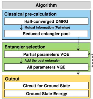
where $Q(\hat{E_{i}})$ denotes the subset of qubits that $\hat{E_{i}}$ acts on and $L(\hat{E_{i}})$ denotes the number of qubits present in $Q(\hat{E_{i}})$. The correlation strength can be regarded as the average MI of qubit pairs within $Q(\hat{E_{i}})$. In our method, we first approximate the ground state wavefunction and the MI of all qubit pairs in it by DMRG (or other classical methods). Then, we calculate the correlation strength defined in Eq. (5) for the entanglers and rank the entanglers according to their correlation strengths from high to low. Finally, we empirically choose first $p_{\text{cut}}$ percent of entanglers and place them into a new reduced pool. We formally summarize our MI-assisted adaptive VQE above, accompanied by an illustration in Fig. (1).

1. Prepare the qubit Hamiltonian $\hat{H}$ to solve. Set the correlation strength cutoff percentile $p_{\text{cut}}$.

2. Define the original entangler pool $E_{\text{original}}=\{\hat{E_{i}}\}$.

3. Calculate ground state of $\hat{H}$ by DMRG and use the DMRG wavefunction to calculate the MI defined in Eq. (3) of all qubit pairs.

4. Calculate the correlation strength defined in Eq. (5) of all the entanglers in the pool. Select $p_{\text{cut}}$ percent of the entanglers that have the largest correlation strength.

5. Discard all the entanglers in $E_{\text{original}}$ which is not selected in the previous step. Denote the new entangler pool by $E_{\text{screened}}$.

6. Carry out the adaptive ansatz construction with $E_{\text{screened}}$

Protocol 1 MI-assisted adaptive VQE

III Numerical Examples

Figure 2: The screening rate $p_{\text{max}}$ of the (a) $\mathrm{H_{2}}$ and (b) $\mathrm{LiH}$ molecule plotted against the bond lengths of the molecules. In our method, by a screened pool with $p_{\text{max}}N(E_{\mathrm{original}})$ entanglers, a calculation the same as using the original entangler pool can be achieved. The number of qubits used in each setting is specified in the parentheses.

molecule	$\mathrm{H_{2}}$	$\mathrm{LiH}$	$\mathrm{H_{2}O}$
molecular configuration	$d(\mathrm{HH})\in[0.6,1.8]$	$d(\mathrm{LiH})\in[1.2,2.4]$	$d(\mathrm{OH})\in[1.2,2.4],\angle\mathrm{HOH}=107.6^{\circ}$
atomic basis set	6-31g	sto-3g	6-31g
complete active space (CAS)	2e/4orb(Full)	2e/3orb(A1:3)	4e/5orb(B2:2,A1:3)
fermion-to-qubit mapping	BK,JW,parity	BK,JW,parity	parity
number of qubits	6,7,8	4,5,6	8
spin-orbital grouping	$\alpha\beta\alpha\beta,\alpha\alpha\beta\beta$	$\alpha\beta\alpha\beta,\alpha\alpha\beta\beta$	$\alpha\alpha\beta\beta$

Table 1: Detailed information of the numerical experiments.

We demonstrate our MI-assisted adaptive VQE with the QCC entangler pool, in which the entanglers are all the exponentiated Pauli words $\exp(-i\hat{P}\tau)$. We run our method on three molecules: $\mathrm{H_{2}}$, $\mathrm{LiH}$ and $\mathrm{H_{2}O}$. Because digital quantum computer cannot directly process creation and annihilation operators that are contained in molecular Hamiltonians, a transformation from fermionic Hamiltonians into qubit Hamiltonians is needed. In this work, Jordan-Wigner (JW) Wigner and Jordan (1928), parity and Bravyi-Kitaev (BK) Bravyi and Kitaev (2002) transformations are used and compared. Furthermore, because there is no external magnetic field in the systems considered, we screen all the entanglers containing even number of Pauli $Y$ operators because they commute with $\hat{H}$, as in Ref. Ryabinkin et al. (2020).

The parameters of the calculations are listed in Table 1. The fermion-qubit transformations are implemented by OpenFermion McClean et al. (2020); the quantum circuit simulation is implemented by ProjectQ Steiger et al. (2018) and the DMRG calculation is carried out by iTensor ITe . All the optimizations are done by the basin-hopping method Wales (2004) from SciPy Virtanen et al. (2020) with heuristic parameters of 10 iterations, 0.5 temperature and $10^{-6}$ step size. Chemical accuracy is defined to be 1 milihartree compared to the full configuration interaction (FCI) energy within certain basis set and active space. The FCI calculations are done by PySCF Sun et al. (2018); Sun (2015).

Figure 3: The screening rate $p_{\text{avg}}$ of the (a) $\mathrm{H_{2}}$ and (b) $\mathrm{LiH}$ molecule plotted against the bond lengths of the molecules. The low $p_{\text{avg}}$ of a run implies that the entanglers added in the circuit of the run tend to have high correlation strength overall. The number of qubits used in each setting is specified in the parentheses.

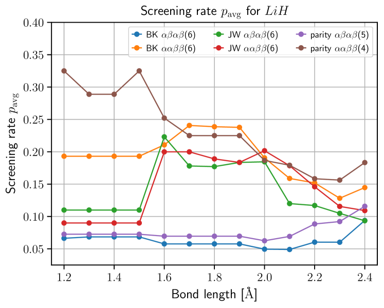
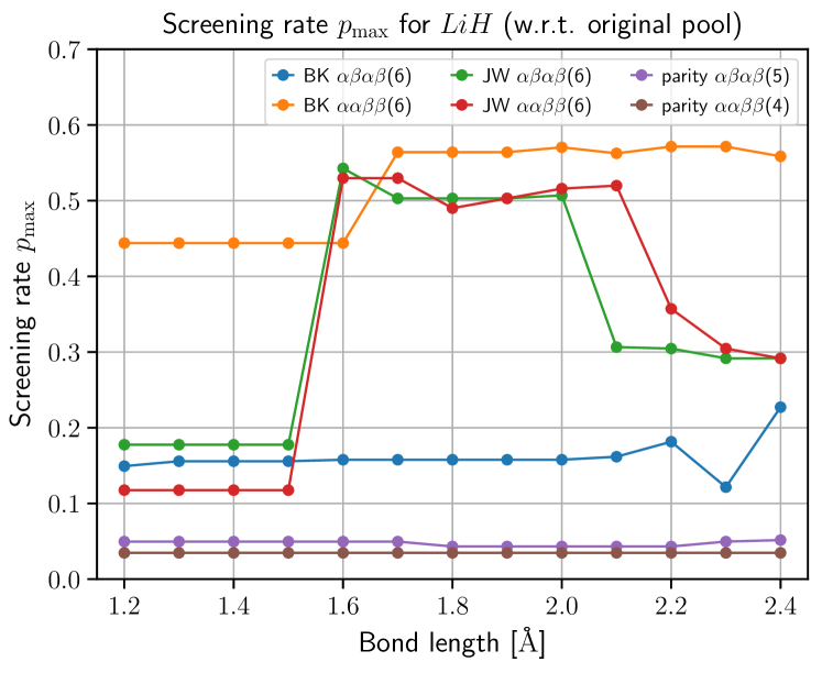
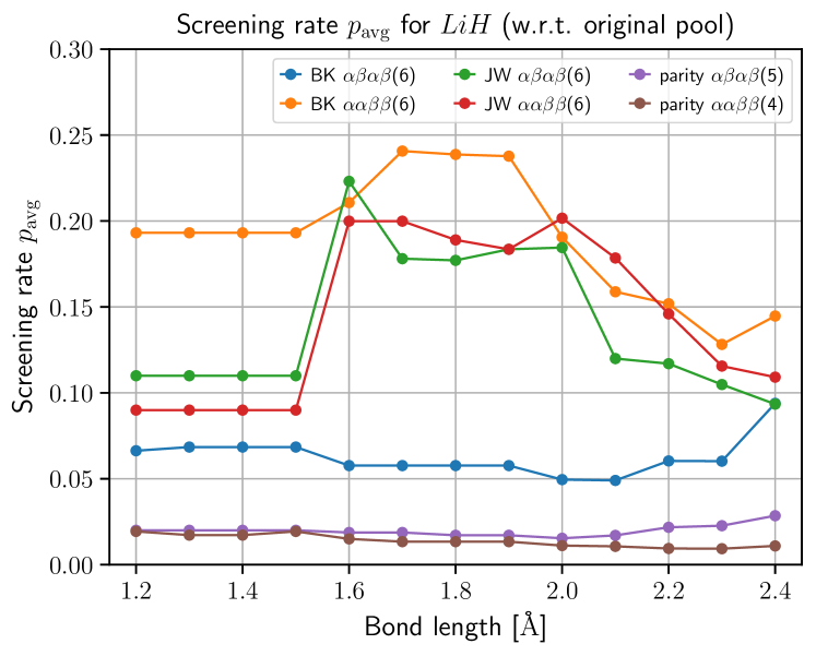
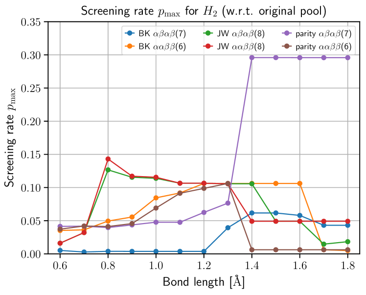
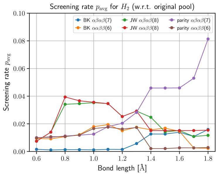
To evaluate the performance of our method, we need to estimate how the correlation strength of an entangler is related to its possibility to be added in the ansatz in the adaptive construction process. If the correlation strength of the selected entanglers are relatively high, removing the entanglers with low correlation strength will make no difference to the ansatz construction because they will not be added to the ansatz. For this reason, we define a quantity, correlation percentile, or simply percentile, on the entanglers in an entangler pool. For an entangler $\hat{E}_{i}$, suppose there are $N_{\geq}(\hat{E_{i}})$ entanglers whose correlation strength is larger or equal to $\hat{E_{i}}$’s. We define its percentile $\mathcal{P}(\hat{E_{i}})$ as $N_{\geq}(\hat{E_{i}})/N(E_{\mathrm{origin}})$, where $N(E)$ denotes the size of the entangler pool $E$. In the demonstration of our method, we record the percentile of every selected entangler and present analysis of a run based on them. Especially, we define and track the screening rates $p_{\text{max}}$ and $p_{\text{avg}}$. They are computed by the percentiles of the entanglers in the final circuit after convergence in a run is reached. Suppose $\{\hat{U_{i}}\}$ are the entanglers added to the ansatz when the adaptive construction stops. First, we define $p_{\text{max}}$ as

$$p_{\text{max}}=\max_{i}\mathcal{P}(\hat{U_{i}}),$$ (6)

which is the highest percentile of the entanglers in the ansatz. $p_{\text{max}}$ can also be understood as the percentile of the selected entangler with lowest correlation strength in the final circuit. Similar to $p_{\text{max}}$, we also define $p_{\text{avg}}$ as

$$p_{\text{avg}}=\frac{1}{N_{\mathrm{ent}}}\sum_{i}\mathcal{P}(\hat{U_{i}}),$$ (7)

which is the average value of the percentiles of all the selected entanglers $N_{\mathrm{ent}}$. Both $p_{\text{max}}$ and $p_{\text{avg}}$ represent how the correlation strength of the selected entanglers are larger than that of the not selected ones, and provide ways to quantify speed-ups compared to a complete entangler pool. Therefore, we call them screening rates. As long as $p_{\text{cut}}$ is set to be higher than $p_{\text{max}}$, the entangler selection at each step will be the same as using the original pool. A low $p_{\text{max}}$ means a low $p_{\text{cut}}$ can be set and one only needs to try a small portion of entanglers in the original pool. Suppose $N_{\mathrm{ent}}$ entanglers were to be added eventually. With the knowledge of $p_{\text{max}}$, one would need to carry out $p_{\text{max}}N(E_{\mathrm{origin}})$ entangler trials at each step. In total, we only need to carry out $N_{\max}=p_{\text{max}}N(E_{\mathrm{origin}})N_{\mathrm{ent}}$ entangler trials in the entire calculation. From our numerical experiments, we find that $p_{\text{max}}$ is nearly continuous with respect to the geometry of the molecular system in some cases. However, we do not know how to predict $p_{\text{max}}$ systematically. When $p_{\text{max}}$ cannot be accurately predicted, $p_{\text{cut}}$ may be set heuristically. As to $p_{\text{avg}}$, different from $p_{\text{max}}$, we cannot use a fixed screened pool with $N_{\mathrm{avg}}=p_{\text{avg}}N(E_{\mathrm{original}})$ entanglers to recover the entangler selection using the original pool because in some steps we need a pool with $N_{\max}$ entanglers to recover the selection. However, we expect that by adjusting the screened pool at each step using some sophisticated techniques, with an average pool size between $N_{\mathrm{avg}}$ and $N_{\max}$, one can recover the original entangler selection.

In all of our numerical experiments, we terminate the calculations when the chemical accuracy is reached. Different from the describe in Protocol 1, we run the adaptive construction with a complete entangler pool in order to show the percentiles of the selected entanglers and how low $p_{\text{cut}}$ can be set for those systems. In addition, we are only interested in whether the entanglers of low percentile are likely to provide a relatively large energy descent and do not concern whether their energy descent is exactly the largest. Therefore, we do not insist on adding the entangler whose energy descent is the largest at each step. Instead, we regard all the entanglers that give an energy descent larger than $30\%$ of the largest energy descent as acceptable entanglers and then we add the entangler with the largest correlation strength among all the acceptable entanglers. This strategy is adopted across all the numerical experiments.

III.1 $\mathrm{H_{2}}$ and $\mathrm{LiH}$ molecules

We carry out our proposed method on $\mathrm{H_{2}}$ and $\mathrm{LiH}$ molecules with basis and active space specified in Table 1. The bond lengths are chosen from 0.6 $\AA$ to 1.8 $\AA$ for $\mathrm{H_{2}}$ and 1.2 $\AA$ to 2.4 $\AA$ for $\mathrm{LiH}$, respectively. The orbitals are ordered by their energy before the fermion-qubit transformation. We compare the results obtained from different transformations as well as different grouping of spin-orbitals before the transformation. Particularly, we study the $\alpha\alpha\beta\beta$ grouping and $\alpha\beta\alpha\beta$ grouping. In the $\alpha\alpha\beta\beta$ grouping, spin-orbitals of $\alpha$ spin are placed first, followed by the $\beta$ spin. In the $\alpha\beta\alpha\beta$ grouping, spin-orbitals with $\alpha$ and $\beta$ spins are placed alternately. In the runs, the number of qubits needed depends on the fermion-qubit transformation and the size of the entangler pools of the runs are determined by its qubit number. The run with 4, 5, 6, 7 and 8 qubits uses a pool with 120, 496, 2016, 8128 and 32640 entanglers respectively.

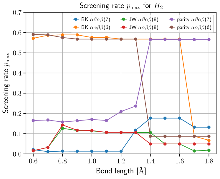
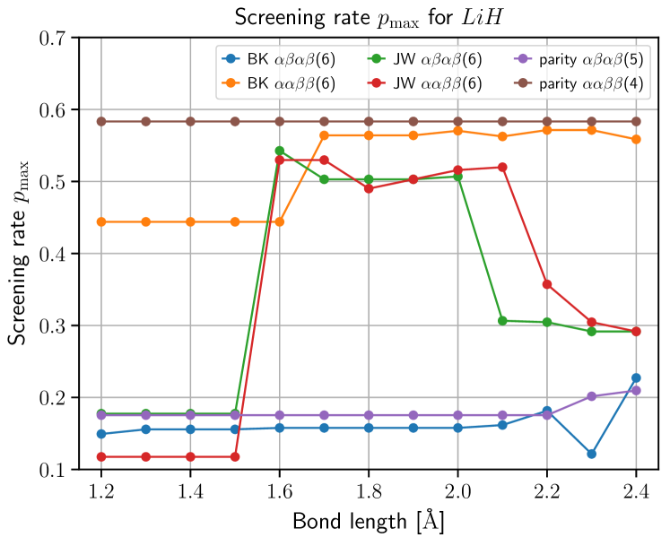
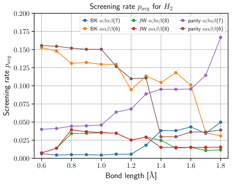
The results from all those numerical simulations are presented in Figs. (2) and (3). We find that the resulting percentiles can be very low for both $\mathrm{H_{2}}$ and $\mathrm{LiH}$ molecules in some cases, meaning we can neglect most part of the original pool and a significant speed-up can be achieved. For example, for $\mathrm{H_{2}}$ with BK $\alpha\beta\alpha\beta$ (Bravyi-Kitaev transformation with $\alpha\beta\alpha\beta$ grouping), $p_{\text{max}}$ can be around $1.5\%$ for some bond lengths (see Fig. (2)(a)), showing that in these settings high correlation strength strongly correlates with high energy descent. In addition, it also implies that the original entangler pool can be reduced to $1.5\%$ of its original size. Besides $p_{\text{max}}$, the $p_{\text{avg}}$ of the runs, which are less than half of the corresponding $p_{\text{max}}$ in most of the cases, also show that the entanglers in the runs are mainly placed among the qubits with high correlation strength. We notice that for different transformations and bond lengths our method can give disparate screening rates and in some cases the screening rate $p_{\text{max}}$ is higher than $50\%$. However, we want to point out that, for most of the systems with high screening rate, the pools have already been reduced by removing stationary qubits and the screening rates are with respect to the already reduced pools. If the screening rates are computed with respect to the original 8-qubit (for $\mathrm{H_{2}}$) and 6-qubit (for $\mathrm{LiH}$) pools, BK $\alpha\beta\alpha\beta$ still presents lowest $p_{\text{max}}$ for $\mathrm{H_{2}}$ in bond length less or equal to $1.3\AA$. But for $\mathrm{LiH}$ and $\mathrm{H_{2}}$ in bond length larger than $1.3\AA$, the encoding with lowest $p_{\text{max}}$ becomes parity $\alpha\alpha\beta\beta$. The screening rates computed in this way are given in the appendix. A detail worth mentioning here is that the orbitals of $\mathrm{H_{2}}$ have different irreducible representations and a orbital ordering change happens in the bond length interval from $1.3\AA$ to $1.4\AA$. This might be in part responsible for the change of $p_{\text{max}}$ there for some transformations. In contrast, the orbitals of $\mathrm{LiH}$ all have the same irreducible representations. Based on the above observation, we believe that a proper transformation, concerning spin-orbital grouping and orbital ordering, should be chosen based on the system for our method. For a clearer picture, more in depth benchmarks will be necessary.

III.2 $\mathrm{H_{2}O}$ molecule

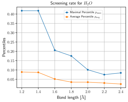
We further evaluate the performance of our method on $\mathrm{H_{2}O}$ with bond angle $\angle\mathrm{HOH}=107.6^{\circ}$ and bond length ranging from 1.2 $\AA$ to 2.4 $\AA$. The basis and transformation used is 6-31g and the parity transformation. 8 qubits are needed after choosing an active space specified in Table 1 and reducing 2 stationary qubits by $\alpha\alpha\beta\beta$ grouping combined with the parity transformation Bravyi et al. (2017). The number of entanglers in the complete 8-qubit pool is $32640$. We add a spin penalty term $S^{2}$ to the original Hamiltonian to help the calculation converge when the bond length is larger or equal to $1.8\AA$. In this setting, $p_{\text{max}}$ and $p_{\text{avg}}$ both show a decreasing trend as the bond length grows. Especially, $p_{\text{max}}$ and $p_{\text{avg}}$ for bond length 2.4 $\AA$ is only $8.44\%$ and $2.44\%$ (see Fig. (4)), meaning that our method can greatly reduce the size of the entangler pool for the stretched water system, where the correlation energy is large.

Figure 4: The screening rate $p_{\text{max}}$ and $p_{\text{avg}}$ for the $\mathrm{H_{2}O}$ molecule with different bond lengths.

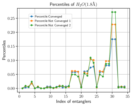
Due to the relatively large correlation energy present in $\mathrm{H_{2}O}$, the numbers of entanglers needed to converge to chemical accuracy are larger than that for $\mathrm{H_{2}}$ and $\mathrm{LiH}$, providing good examples to show the stability of percentiles in our method with inaccurate MI. Let us take the water molecule with bond length 1.8 $\AA$ as an example. In this case, 34 entanglers are used for chemical accuracy. In Fig. (5), we show how the percentile varies by using MI from DMRG calculations of different convergence level. We included three curves, one for a converged calculation whose energy is within 1 milihartree from the FCI energy, one about 10 milihartree and one about 20 milihartree from the FCI energy. We find that for the first 16 entanglers, where the percentiles are comparatively low, the difference is not significant. The deviation becomes apparent when the percentile is high. However, in the worst case, the MI from the non-converged DMRG calculation only lift the $p_{\text{max}}$ of this run from $17.5\%$ to $27.2\%$. Considering the large deviation of energy from the FCI, we claim that in this run non-converged DMRG still provides a good MI estimation. This is vital for our method to be applied to larger system where accurate estimations of MIs are expected to be challenging.

Figure 5: Percentiles of entanglers in run for the $\mathrm{H_{2}O}$ molecule with bond length of $1.8$ $\AA$. The index represents the order of adding the entanglers. The entangler with smaller index is added earlier in the run. The energy of the run Not converged 1 and Not converged 2 are about 10 milihartree and 20 milihartree away from the (Converged) FCI energy respectively.

IV Conclusions

In the present work, we provide a mean to reduce the size of the entangler pools for adaptive ansatz construction methods in VQE using MI which can be approximated by existing classical algorithms such as DMRG. Our method reveals how MI can help to construct the ansatz for VQE. In our numerical experiments, the best case scenario only requires about $1.5\%$ of the original entangler pool to achieve the same numerical accuracy. We also find that the average correlation strength $p_{\text{avg}}$ can be very low for a system, which implies that the entanglers should be mainly placed among the qubits in which the MI between the qubits is high. Further, the screening rates are not independent of the chosen fermion-qubit transformation and disparate $p_{\text{max}}$ and $p_{\text{avg}}$ are observed for different transformations, providing an additional criterion to quantify the performance of different transformations Tranter et al. (2018).

Although low percentile means high speed-up comparing to the original QCC in our method, it remains unknown that whether low percentile means also low difficulty for classical computers to simulate. It will be interesting to bridge the two percentile values $p_{\text{max}}$ and $p_{\text{avg}}$ we define, with classical resource needed for simulation. If low $p_{\text{max}}$ was associated with low difficulty in classical simulation, $p_{\text{max}}$ could be a new quantifier to indicate the difficulty of simulating a system classically. If the converse was true, a system with low $p_{\text{max}}$ and high difficulty to simulate classically would be a good problem choice to demonstrate quantum advantage over the classical counterpart.

Appendix

Figure 6: The screening rates $p_{\text{max}}$ and $p_{\text{avg}}$ for $\mathrm{LiH}$ with respect to the 6-qubit original pool (2016 entanglers).

Figure 7: The screening rates $p_{\text{max}}$ and $p_{\text{avg}}$ for $H_{2}$with respect to the 8-qubit original pool (32640 entanglers).

References

- Nielsen and Chuang (2002) M. A. Nielsen and I. Chuang, Quantum Computation and Quantum Information (Cambridge University Press, 2002).
- Shor (1994) P. W. Shor, “Algorithms for quantum computation: discrete logarithms and factoring,” Proceedings 35th annual symposium on foundations of computer science , 124 (1994).
- Harrow et al. (2009) A. W. Harrow, A. Hassidim, and S. Lloyd, “Quantum algorithm for linear systems of equations,” Phys. Rev. Lett. 103, 150502 (2009).
- Arute et al. (2019) F. Arute, K. Arya, R. Babbush, D. Bacon, J. C. Bardin, R. Barends, R. Biswas, S. Boixo, F. G. Brandao, D. A. Buell, et al., “Quantum supremacy using a programmable superconducting processor,” Nature 574, 505 (2019).
- Wright et al. (2019) K. Wright, K. Beck, S. Debnath, J. Amini, Y. Nam, N. Grzesiak, J.-S. Chen, N. Pisenti, M. Chmielewski, C. Collins, et al., “Benchmarking an 11-qubit quantum computer,” Nature Comm. 10, 1 (2019).
- Gong et al. (2019) M. Gong, M.-C. Chen, Y. Zheng, S. Wang, C. Zha, H. Deng, Z. Yan, H. Rong, Y. Wu, S. Li, F. Chen, Y. Zhao, F. Liang, J. Lin, Y. Xu, C. Guo, L. Sun, A. D. Castellano, H. Wang, C. Peng, C.-Y. Lu, X. Zhu, and J.-W. Pan, “Genuine 12-qubit entanglement on a superconducting quantum processor,” Phys. Rev. Lett. 122, 110501 (2019).
- Preskill (2018) J. Preskill, “Quantum computing in the nisq era and beyond,” Quantum 2, 79 (2018).
- Atkins and Friedman (2011) P. W. Atkins and R. S. Friedman, Molecular quantum mechanics (Oxford university press, 2011).
- Helgaker et al. (2014) T. Helgaker, P. Jorgensen, and J. Olsen, Molecular electronic-structure theory (John Wiley & Sons, 2014).
- Reiher et al. (2017) M. Reiher, N. Wiebe, K. M. Svore, D. Wecker, and M. Troyer, “Elucidating reaction mechanisms on quantum computers,” Proc. Natl. Acad. Sci. U.S.A. 114, 7555 (2017).
- Cao et al. (2019) Y. Cao, J. Romero, J. P. Olson, M. Degroote, P. D. Johnson, M. Kieferová, I. D. Kivlichan, T. Menke, B. Peropadre, N. P. Sawaya, et al., “Quantum chemistry in the age of quantum computing,” Chem. Rev. 119, 10856 (2019).
- McArdle et al. (2020) S. McArdle, S. Endo, A. Aspuru-Guzik, S. C. Benjamin, and X. Yuan, “Quantum computational chemistry,” Rev. Mod. Phys. 92, 015003 (2020).
- Peruzzo et al. (2014) A. Peruzzo, J. McClean, P. Shadbolt, M.-H. Yung, X.-Q. Zhou, P. J. Love, A. Aspuru-Guzik, and J. L. O’brien, “A variational eigenvalue solver on a photonic quantum processor,” Nature comm. 5, 4213 (2014).
- McClean et al. (2016) J. R. McClean, J. Romero, R. Babbush, and A. Aspuru-Guzik, “The theory of variational hybrid quantum-classical algorithms,” New J. Phys. 18, 023023 (2016).
- Kandala et al. (2017) A. Kandala, A. Mezzacapo, K. Temme, M. Takita, M. Brink, J. M. Chow, and J. M. Gambetta, “Hardware-efficient variational quantum eigensolver for small molecules and quantum magnets,” Nature 549, 242 (2017).
- Romero et al. (2018) J. Romero, R. Babbush, J. R. McClean, C. Hempel, P. J. Love, and A. Aspuru-Guzik, “Strategies for quantum computing molecular energies using the unitary coupled cluster ansatz,” Quantum Sci. Technol. 4, 014008 (2018).
- Ryabinkin et al. (2018) I. G. Ryabinkin, T.-C. Yen, S. N. Genin, and A. F. Izmaylov, “Qubit coupled cluster method: A systematic approach to quantum chemistry on a quantum computer,” Journal of chemical theory and computation 14, 6317 (2018).
- Ryabinkin et al. (2020) I. G. Ryabinkin, R. A. Lang, S. N. Genin, and A. F. Izmaylov, “Iterative qubit coupled cluster approach with efficient screening of generators,” J. Chem. Theory Comput. 16, 1055 (2020).
- Grimsley et al. (2019) H. R. Grimsley, S. E. Economou, E. Barnes, and N. J. Mayhall, “An adaptive variational algorithm for exact molecular simulations on a quantum computer,” Nature comm. 10, 1 (2019).
- Rissler et al. (2006) J. Rissler, R. M. Noack, and S. R. White, “Measuring orbital interaction using quantum information theory,” Chem. Phys. 323, 519 (2006).
- Legeza and Sólyom (2003) O. Legeza and J. Sólyom, “Optimizing the density-matrix renormalization group method using quantum information entropy,” Phys. Rev. B 68, 195116 (2003).
- Stein and Reiher (2019) C. J. Stein and M. Reiher, “autocas: A program for fully automated multiconfigurational calculations,” J. Comput. Chem. 40, 2216 (2019).
- Chan and Sharma (2011) G. K.-L. Chan and S. Sharma, “The density matrix renormalization group in quantum chemistry,” Annu. Rev. Phys. Chem. 62, 465 (2011).
- Amico et al. (2008) L. Amico, R. Fazio, A. Osterloh, and V. Vedral, “Entanglement in many-body systems,” Rev. Mod. Phys. 80, 517 (2008).
- Wigner and Jordan (1928) E. P. Wigner and P. Jordan, “Über das paulische äquivalenzverbot,” Z. Phys 47, 631 (1928).
- Bravyi and Kitaev (2002) S. B. Bravyi and A. Y. Kitaev, “Fermionic quantum computation,” Ann. Phys. 298, 210 (2002).
- McClean et al. (2020) J. R. McClean, N. C. Rubin, K. J. Sung, I. D. Kivlichan, X. Bonet-Monroig, Y. Cao, C. Dai, E. S. Fried, C. Gidney, B. Gimby, et al., “OpenFermion: the electronic structure package for quantum computers,” Quantum Sci. Technol. 5, 034014 (2020).
- Steiger et al. (2018) D. S. Steiger, T. Häner, and M. Troyer, “Projectq: an open source software framework for quantum computing,” Quantum 2, 49 (2018).
- (29) ITensor Library (version 2.0.11) http://itensor.org .
- Wales (2004) D. Wales, Energy Landscapes: Applications to Clusters, Biomolecules and Glasses, Cambridge Molecular Science (Cambridge University Press, 2004).
- Virtanen et al. (2020) P. Virtanen, R. Gommers, T. E. Oliphant, M. Haberland, T. Reddy, D. Cournapeau, E. Burovski, P. Peterson, W. Weckesser, J. Bright, S. J. van der Walt, M. Brett, J. Wilson, K. Jarrod Millman, N. Mayorov, A. R. J. Nelson, E. Jones, R. Kern, E. Larson, C. Carey, İ. Polat, Y. Feng, E. W. Moore, J. Vand erPlas, D. Laxalde, J. Perktold, R. Cimrman, I. Henriksen, E. A. Quintero, C. R. Harris, A. M. Archibald, A. H. Ribeiro, F. Pedregosa, P. van Mulbregt, and S. . . Contributors, “SciPy 1.0: Fundamental Algorithms for Scientific Computing in Python,” Nature Methods 17, 261 (2020).
- Sun et al. (2018) Q. Sun, T. C. Berkelbach, N. S. Blunt, G. H. Booth, S. Guo, Z. Li, J. Liu, J. D. McClain, E. R. Sayfutyarova, S. Sharma, et al., “PySCF: the Python-based simulations of chemistry framework,” Wiley Interdiscip. Rev. Comput. Mol. Sci. 8, e1340 (2018).
- Sun (2015) Q. Sun, “Libcint: An efficient general integral library for gaussian basis functions,” Journal of Computational Chemistry 36, 1664 (2015).
- Bravyi et al. (2017) S. Bravyi, J. M. Gambetta, A. Mezzacapo, and K. Temme, “Tapering off qubits to simulate fermionic hamiltonians,” arXiv:1701.08213 (2017).
- Tranter et al. (2018) A. Tranter, P. J. Love, F. Mintert, and P. V. Coveney, “A comparison of the bravyi–kitaev and jordan–wigner transformations for the quantum simulation of quantum chemistry,” Journal of Chemical Theory and Computation 14, 5617 (2018), pMID: 30189144.