Universal spectral form factor for many-body localization

Abstract

We theoretically study correlations present deep in the spectrum of many-body-localized systems. An exact analytical expression for the spectral form factor of Poisson spectra can be obtained and is shown to agree well with numerical results on two models exhibiting many-body-localization: a disordered quantum spin chain and a phenomenological $l$-bit model based on the existence of local integrals of motion. We also identify a universal regime that is insensitive to the global density of states as well as spectral edge effects.

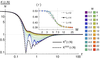
Understanding how thermal equilibrium may, or may not emerge in isolated many-body quantum systems remains a central question in quantum statistical mechanics. Thermal systems which are said to exhibit quantum chaos satisfy the eigenstate thermalization hypothesis (ETH) [1, 2] whose subsystems equilibriate under their own dynamics. In addition to being highly entangled, i.e. satisfying a “volume law” scaling with subsystem size, the eigenspectra of these systems exhibit long range repulsions that are captured by random matrix theory and produce universal features in their correlations measured in their spectral form factor (SFF, defined below in eqs. 4 and 5) such as the linear ramp [3, 4, 5, 6, 7, 8, 9] (as shown in fig. 1). In the presence of strong quenched randomness or quasiperiodicity, quantum systems can become many body localized (MBL) [10, 11, 12, 13] where ETH is violated. In contrast to chaotic systems, MBL is characterized by eigenstates with short-range “area law” entanglement and an absence of level repulsion. Recent experiments on ultra-cold atomic gases [14, 15, 16], trapped ions [17], superconducting qubits [18, 19] and nuclear spins [20] have provided evidence for the existence of the MBL phase.

Instabilities to MBL have been argued to arise in high dimensions [21] and in the presence of certain symmetries [22]. More recently however, the very existence of the MBL phase has been challenged based on a finite size scaling analysis of the linear ramp of the SFF on approach to the MBL transition from the chaotic side [23]. A critique of this work was subsequently presented [24] pointing out the intricacies involved in finite sized calculations and conclusions drawn from them, while further studies have highlighted the difficulty in studying the MBL transition in finite size numerics [25, 26]. Recently, the authors of Ref. [23] pointed out that their claim of the absence of MBL is due to their choice of scaling function, which instead should follow a Kosteritz-Thouless “like” scaling form as they demonstrate in Ref. [27] consistent with recent theories of the MBL transition [28, 29, 30]. Irrespective of the question of validity of the finite-size numerics in the vicinity of the MBL transition, the question of how to characterize the MBL phase using the SFF alone, is undoubtedly worthy of further examination. If the MBL phase indeed exists, it is conceivable that its SFF has its own universal features to which any putative system exhibiting MBL should be compared. However, apart from a few hints [31], the existence of such a form and an understanding of its features has been lacking thus far.

Figure 1: The spectral form factor across the MBL transition. This is defined in eq. 4 and computed from $N=20$ eigenvalues from the center of the many-body spectrum at different disorder strengths $W$ for the Hamiltonian in eq. 1 with a system size $L=14$. (Inset): The adjacent gap ratio, $\langle r\rangle$ defined in eq. 3 versus $W$. The approximate critical disorder, where the data at different system sizes cross is given by $W_{c}\approx 7.3$ has also been marked. For $W\gg W_{c}$ in the MBL phase the level statistics are Poisson $\langle r\rangle=2\ln(2)-1\approx 0.39$  [32]. The dashed black line is the well known GOE expectation from random matrix theory known to describe the thermal phase, whereas the solid black line, that matches the numerical data in the MBL phase well (over the range of $W\geq 10$ [33]), is obtained in eq. 8. The analytical expressions $K^{GOE}(\tau,N)$ and $K^{P}(\tau,N)$ as well as the data are normalized to set the mean level spacing to unity.

In this Letter, we investigate the spectral correlations in MBL systems. We show that the SFF for MBL systems can be calculated deep in the spectrum due to their convergence with Poisson levels for which we can derive an exact analytical expression with a finite number of levels [34], (plotted as a solid line in fig. 1). We determine the validity of this expression by comparing it with numerical simulations of a phenomenological $l$-bit model [35, 36] as well as a microscopic disordered many-body Hamiltonian. In both cases, by focusing on states in the middle of the many body spectra where the many-body density of states is nearly flat, we find excellent agreement between the exact expression and the numerical results. In the limit of an infinite number of levels, to leading order, our results reduce to the general expectation of integrable systems due to Berry and Tabor [37, 38]. However, we show that the leading correction to the SFF beyond that of Berry and Tabor is universal in an intermediate power-law scaling regime and is robust to changes in the global density of states as well as spectral edge effects. Our results provide further support for the existence of the MBL phase in one dimension.

Models for many-body localization: To make a detailed comparison with the properties of the MBL phase, we consider two different models. The first is a quantum spin-chain with quenched disorder whose Hamiltonian is

$$H=\sum_{i}J_{1}(S^{x}_{i}S^{x}_{i+1}+S^{y}_{i}S^{y}_{i+1}+\Delta S^{z}_{i}S^{z}_{i+1})+w_{i}S^{z}_{i}\\ +\sum_{i}J_{2}(S^{x}_{i}S^{x}_{i+2}+S^{y}_{i}S^{y}_{i+2}+\Delta S^{z}_{i}S^{z}_{i+2}).$$ (1)

$S^{\alpha}$ are spin operators that can be written in terms of Pauli matrices as $S^{\alpha}=\frac{1}{2}\sigma^{\alpha}$ and the random couplings $w_{i}$ are drawn from a uniform distribution $[-W,W]$. Variants of this model have been previously studied [23, 39, 40] and are known to have a thermal phase at weak disorder and an MBL phase at strong disorder. Following Ref [23], we set $J_{1}=J_{2}=1.0$ and $\Delta=0.55$.

Deep in the MBL phase, any local Hamiltonian such as eq. 1 can be described by a complete set of emergent local integrals of motion [35, 36]. This means that there should exist a finite depth unitary circuit $U$ that can recast $H$ into a diagonal form, $UHU^{\dagger}=H_{lbit}$:

$$H_{lbit}=\sum_{i}J^{(1)}_{i}\kappa^{z}_{i}+\sum_{i,j}J^{(2)}_{ij}\kappa^{z}_{i}\kappa^{z}_{j}+\sum_{i,j,k}J^{(3)}_{ijk}\kappa^{z}_{i}\kappa^{z}_{j}\kappa^{z}_{k}+\ldots$$ (2)

where $\kappa^{z}_{i}$ are the so called $l$-bit Pauli operators with localized support on the Hilbert space near site $i$, whose eigenvalues represent the locally conserved quantities and the magnitudes of $J^{m}_{i_{1}\ldots i_{m}}$ fall off exponentially with distance. The second model we consider is a truncated version of the above phenomenological $l$-bit model eq. 2 where we retain only up to 10 spin nearest neighbor interactions with all couplings drawn from a uniform distribution $J^{(1\ldots 10)}\in[-1,1]$.

Characterizing spectral correlations of quantum systems: A popular diagnostic used to distinguish MBL and chaotic systems via their spectral correlations is the adjacent gap ratio ($r$)  [32]. This is defined in terms of successive gaps $\delta_{i}=E_{i+1}-E_{i}$ of an ordered energy spectrum $\{E_{i}\}$ as follows:

$$r_{i}=\frac{\mathrm{min}(\delta_{i},\delta_{i+1})}{\mathrm{max}(\delta_{i},\delta_{i+1})}.$$ (3)

For chaotic systems, the value of $\langle r\rangle$ (where $\langle\dots\rangle$ denotes averaging over samples and energy) can be computed from an appropriate random matrix ensemble. For example, the Gaussian orthogonal ensemble (GOE), appropriate for systems with time-reversal symmetry gives $\langle r\rangle\approx 0.53$, while Poisson levels, applicable for MBL systems gives $\langle r\rangle=2\ln(2)-1\approx 0.39$ [32]. As shown in the inset of fig. 1, by tracking $\langle r\rangle$, we can see that the Hamiltonian of eq. 1 supports a thermal phase for small $W$ and an MBL phase for large $W$ with the critical disorder strength somewhere near $W_{c}\approx 7.3$ where the curves for different system sizes cross, consistent with previous work [23].

The adjacent gap ratio captures the repulsion of neighboring levels, and thus only probes local spectral correlations. It does not measure long-range spectral correlations, which have important and useful information. A more comprehensive diagnostic is the spectral form factor (SFF) [3], which is the main tool of analysis in this Letter and is defined in terms of eigenvalues $\{E_{i}\}$ as follows:

$$K(\tau,N)=\langle\sum_{m,n=1}^{N}e^{i\tau(E_{m}-E_{n})}\rangle$$ (4)

where $N$ is the total number of eigenvalues in consideration. Also useful is the connected SFF defined as

$$K_{c}(\tau,N)=\langle\sum_{m,n=1}^{N}e^{i\tau(E_{m}-E_{n})}\rangle-|\langle\sum_{m=1}^{N}e^{i\tau E_{m}}\rangle|^{2}.$$ (5)

The information about long-range correlations is contained in the form of $K(\tau,N)$ interpolating the early and late $\tau$ values of $N^{2}$ and $N$ respectively ($0$ and $N$ for $K_{c}(\tau,N)$). For chaotic systems, just like $\langle r\rangle$, the SFF can also be computed from an appropriate random matrix ensemble. For instance, as seen in fig. 1, the SFF for the Hamiltonian eq. 1 with weak disorder strength ($W$) exhibits a clear ramp and matches that of the GOE ensemble whose approximate expression (plotted as a dotted line) is known [3, 4, 5, 6, 7, 8, 9]

As we increase the disorder strength, as shown in fig. 1, the SFF qualitatively changes as the model passes through the MBL transition with the disappearance of the ramp. Deep in the MBL phase (i.e. where $\langle r\rangle\approx 0.39$), the SFF again takes on a new stable form $K^{P}(\tau,N)$ (plotted as a solid black line in fig. 1). The expression for $K^{P}(\tau,N)$ as well as the connected version, $K_{c}^{P}(\tau,N)$ we obtain are presented in eqs. 8 and 9. We will show in the following section that they correspond to energy levels drawn from a Poisson process.

Contrasting features between $K^{GOE}$ and $K^{P}$ can be seen at intermediate $\tau$ values, in the regime where the SFF is expected to be universal (this occurs in the range $\frac{1}{\mu\mathcal{D}}\lesssim\tau\lesssim 1/\mu$ for $K^{GOE}$ and $\frac{1}{\sqrt{\mu\mathcal{D}}}\lesssim\tau\lesssim 1/\mu$ for $K^{P}$ [33]) where $\mathcal{D}=\mu N$ is the many-body bandwidth of the chosen levels and $\mu$ is the mean level spacing. For $K^{GOE}$, this corresponds to the ‘ramp’ region [3, 4, 5, 6, 7, 8, 9]). On the other hand, as expected, $K^{P}(\tau,N)$ lacks the ramp but exhibits a universal sub leading power-law form that will be discussed later.

SFF for Poisson levels: The single-particle spectrum of the Anderson insulator [41] deep in the localized phase can simply be described by a set of uncorrelated random numbers (the values of random chemical potentials). In this case, on scales smaller than the single-particle bandwidth, the spectrum looks like a Poisson process [42, 3]. For example, the distribution of the level spacings is exponential $P(\delta)=\frac{1}{\mu}\exp\left(-\frac{\delta}{\mu}\right)$. Consistent with the hypothesis of emergent integrability in localized systems, this is identical to the distribution of level spacings in point particle systems with integrable classical trajectories conjectured by Berry and Tabor [37, 38] and has been verified in several systems [43, 44].

The many body levels of the Anderson insulator on the other hand is a weighted sum of the single particle eigenvalues. For a system of size $L$, the $\sim\mathcal{O}(L)$ random numbers present in the Hamiltonian are used to generate $\sim 2^{L}$ many-body eigenvalues and are no longer completely uncorrelated. How the spectrum further changes in the presence of interactions for MBL systems is less obvious. However, extensive work [45, 32, 46, 47, 48] has provided evidence that the Poisson nature continues to persist in the many-body levels of MBL systems on energy scales smaller than the many-body bandwidth [32]. To compute the SFF, we need more information than local statistics such as the level spacing distribution - we need the joint distribution of eigenvalues $P(E_{n},n;E_{m},m)$ i.e. the likelihood of the $n^{th}$ level to be $E_{n}$ when the $m^{th}$ level is $E_{m}$. For Poisson process, this is  [33] (assuming $m>n$)

$$P(E_{n},n;E_{m},m) =p(E_{n},n)~{}p(E_{m}-E_{n},m-n)$$ (6)

where $p(E_{k},k)$ is the well known Poisson distribution

$$p(E_{k},k)=\frac{e^{-\frac{E_{k}}{\mu}}}{\mu(k-1)!}\left(\frac{E_{k}}{\mu}\right)^{k-1}.$$ (7)

Using this, we can exactly obtain the expressions for the Poisson SFF [33].

$$K^{P}(\tau,N) =N+\frac{2}{(\mu\tau)^{2}}-\frac{(1+i\mu\tau)^{1-N}+(1-i\mu\tau)^{1-N}}{(\mu\tau)^{2}}$$ (8)

$$K^{P}_{c}(\tau,N) =N+\frac{1}{(\mu\tau)^{2}}-\frac{(1+(\mu\tau)^{2})^{-N}}{(\mu\tau)^{2}}$$

$$~{}~{}~{}~{}~{}~{}~{}~{}~{}~{}~{}-\frac{i}{\mu\tau}\left[(1+i\mu\tau)^{-N}-(1-i\mu\tau)^{-N}\right]$$ (9)

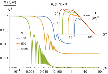
Note that these expressions have been also obtained by the authors of [34] as a special case of a more general result applicable to spectra with uncorrelated gaps. Our focus is on the application of these results to the MBL spectrum where the Poisson nature is emergent and not intrinsic.We now proceed to understand various limiting regimes of the above expressions. In the limit of $N\rightarrow\infty$ we obtain the expected result of Berry-Tabor $\lim_{N\rightarrow\infty}K^{P}(\tau,N)/N=1+\delta(\tau)$. If $\mathcal{D}=\mu N$ is the bandwidth of the selected eigenvalues with mean level spacing $\mu$, the early $\tau$ behavior ($\tau<\frac{1}{\sqrt{\mu\mathcal{D}}}$) is largely determined by the Poisson density of states (DOS) [33] which is non-trivial only at the edges, and is not a universal feature. Just as in the case of RMT, the interesting part is at intermediate values of $\tau$ i.e. $\frac{1}{\sqrt{\mu\mathcal{D}}}<\tau<\frac{1}{\mu}$ (see fig. 2 and [33] for details of various universal and non-universal $\tau$ regimes), where we have

$$K^{P}_{c}(\tau,N)=N+\frac{1}{(\mu\tau)^{2}}+\mathcal{O}\left(\frac{1}{N}\right),$$ (10)

and the disconnected part behaves similarly $K^{P}(\tau,N)-N\sim 2/(\mu\tau)^{2}$. The leading $N$ is merely the large $\tau$ value and is frequently quoted as the SFF signature of Poisson spectra. More interesting is the sub leading $\frac{1}{(\mu\tau)^{2}}$ term that is $N$ independent.

Figure 2: SFF for Poisson levels (Above:) The SFF for Poisson levels for various values of $N$. The reduced SFF $K_{c}(\tau)-N$ exposes the universal form (dashed lines) which sets in after a time $\mu\tau=\frac{1}{\sqrt{N}}$ (marked for each $N$) is shown in the inset. (Below:) The various universal and non-universal $\tau$ regimes are shown for the connected SFF.

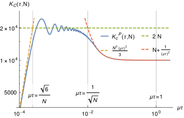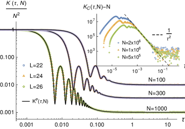
This suggests that if we subtract the dominant trivial value and consider $K_{c}(\tau,N)-N$ which we dub the reduced SFF, it should assume a $\frac{1}{(\mu\tau)^{2}}$ form that survives the $N\rightarrow\infty$ limit and is universal in the same way that the ramp is universal to RMT i.e. the form is robust to effects from spectral edges arising from a finite bandwidth as well as non-trivial global density of states [4]. Note that similar time-scales as well as scaling forms were also obtained in [34] even though their notion of universality (independence of underlying gap distribution) is different from ours [33]. We verify this using the physical models mentioned before where non-negligible edge and DOS effects are expected.

Comparison with numerical calculations: We now numerically check the analytical results of the previous section by focusing on the two models defined in eq. 1 and eq. 2. Both models possess a global $U(1)$ spin rotation symmetry which allows us to focus on half-filling i.e. the total $S^{z}=0$ sector. We will perform our analysis by shifting the $N$ chosen eigenvalues by the smallest one so as to make them non-negative. For ease of comparison with the analytical results as well as across system sizes, after averaging over disorder samples, we re-scale $\tau$ by the mean level spacing $\mu$ effectively setting $\mu=1$. Depending on system size, our analysis is performed using disorder samples ranging from $10,000$ to $50,000$ [33].

Figure 3: Comparing the SFF for Poisson levels with models of MBL. The SFF for the $l$-bit model of eq. 2 (above) and the microscopic Hamiltonian in eq. 1 deep in the MBL phase with $W=25$ (below) for various system sizes ($L$) and small numbers of eigenvalues ($N$) drawn from the middle of the many-body spectrum compared with the analytical curves $K^{P}(\tau,N)$ of eq. 8. Deviations appear at short $\tau$ but are absent in the universal regime at intermediate $\tau$. Reduced SFF shown for large values of $N$ for the $L=26$ $l$-bit model (inset, above) and $L=18$ Hamiltonian $H(W)$ (inset, below) that clearly demonstrates the universal $1/\tau^{2}$ behavior at intermediate $\tau$.

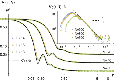It is a well known challenge to compare exact random matrix theory predictions with numerics on microscopic models due to the difference in their DOS, particularly at the edges of the spectral bandwidth. The early $\tau$ behavior of the SFF in particular deviates from the RMT prediction due to this and a better agreement can be obtained by a careful unfolding of the spectrum [50, 3]. However, as the authors of Ref [5] point out, at intermediate values of $\tau$, the ramp is robust to these effects and can be observed even without unfolding. Coming to our Poisson case, the situation is similar - the early $\tau$ behavior is affected by the overall DOS of the microscopic models and thus deviates from the analytical form of $K^{P}(\tau,N)$ in eq. 8. For a fixed number of eigenvalues $N$, these deviations are reduced by increasing the system size $L$ (and thus the total Hilbert space $\mathcal{N}_{L}$). In the thermodynamic limit ($L\rightarrow\infty$) when the parameter $\zeta\equiv N/\mathcal{N}_{L}$ vanishes for any finite $N$, we expect any deviations to completely vanish and the analytical results to match exactly [33]. Nevertheless, as suggested previously, even for large values of $N$ when the early $\tau$ form deviates significantly, the SFF matches at intermediate-$\tau$ values where the SFF is universal and is best seen by in the reduced SFF, $K_{c}(\tau,N)-N$.

We start with the $l$-bit model of eq. 2. Since it is already diagonal, the eigenvalues are generated easily and as a result, we are able to reach relatively large system sizes. As seen in  fig. 3 (top panel), the numerical SFF, $K(\tau,N)$ matches the analytical one for Poisson levels, $K^{P}(\tau,N)$ of eq. 8 (dotted lines) very well with negligible deviations for small values of $N$. For $N\sim 1000$, deviations start becoming visible at short-$\tau$. The universal intermediate-$\tau$ form is very clearly seen at large $N$ in the reduced SFF (inset, top panel) as this expands the universal temporal regime $\frac{1}{\sqrt{\mu\mathcal{D}}}<\tau<\frac{1}{\mu}$.

We now turn to the microscopic Hamiltonian eq. 1 and focus deep in the MBL phase at $W=25$, where $\langle r\rangle\approx 0.39$ is nicely Poisson at the accessible $L$. Here, we are relatively limited in the system sizes that we can reach and the presence of complex microscopic details further impacts the finite sized numerical results more severely than in the case of the idealized $l$-bit model. Nevertheless, as seen in fig. 3 (lower panel), for small values of $N$ (20,40), the numerical SFF matches the analytical equation eq. 8 (dotted lines) very well. For larger values of $N\sim 80$, deviations start becoming visible at short $\tau$ values. Again, the universal intermediate-$\tau$ form is very clearly seen at large $N$ (inset, bottom panel). Although we have only presented the analysis for $W=25$, we find that all these results remain virtually unchanged for a wide range of disorder strengths, $W\geq 10$ [33]. This strongly supports the notion that MBL is a robust phase in disordered one-dimensional isolated quantum many-body systems.

Conclusion: In this Letter, we have derived an exact expression for the spectral form factor of Poisson levels and identified a universal regime. We have shown that this describes the SFF in the many body localized phase well through a detailed comparison with numerical results on two separate physical models. The analytic expression of the spectral form factor obtained here is expected to apply to any integrable many-body quantum system. In particular, we conjecture that in the SFF of integrable models, the universal power-law correction should be observed as a refined version of the Berry-Tabor conjecture.

Note added: During the later stages of our work, we became aware of a recent mathematical physics paper [34] which also comprehensively discusses the spectral form factor for spectra with uncorrelated spacings in a distinct context. At the time of submission, we were also made aware of ref [51] which has some overlapping results presented in the Supplemental Materials [33].

Acknowledgments: We acknowledge helpful discussions with Anirban Basak, Po-Yao Chang, Arghya Das, Subroto Mukerjee, Tomaz Prosen, Sthitadhi Roy, and Marko Znidaric. This work was initiated at the Aspen Center for Physics, which is supported by National Science Foundation Grant No. PHY-1607611. A.P. receives funding from the Simon’s foundation through the ICTS-Simons prize postdoctoral fellowship. M.K. acknowledges support via a Ramanujan Fellowship (SB/S2/RJN-114/2016), an Early Career Research Award (ECR/2018/002085) and a Matrics Grant (MTR/2019/001101) from the Science and Engineering Research Board (SERB), Department of Science and Technology, Government of India. A.P. and M.K. acknowledge support of the Department of Atomic Energy, Government of India, under Project No. RTI4001. J.H.P. is partially supported by NSF Career Grant No. DMR-1941569.

References

- Srednicki [1994] M. Srednicki, Chaos and quantum thermalization, Phys. Rev. E 50, 888 (1994).
- Srednicki [1999] M. Srednicki, The approach to thermal equilibrium in quantized chaotic systems, Journal of Physics A: Mathematical and General 32, 1163 (1999).
- Haake [2010] F. Haake, Quantum Signatures of Chaos, Vol. 54 (2010).
- Cotler et al. [2017] J. Cotler, N. Hunter-Jones, J. Liu, and B. Yoshida, Chaos, complexity, and random matrices, Journal of High Energy Physics 2017, 10.1007/jhep11(2017)048 (2017).
- Gharibyan et al. [2018] H. Gharibyan, M. Hanada, S. H. Shenker, and M. Tezuka, Onset of random matrix behavior in scrambling systems, Journal of High Energy Physics 2018, 124 (2018).
- Liu [2018] J. Liu, Spectral form factors and late time quantum chaos, Phys. Rev. D 98, 086026 (2018).
- Chen and Ludwig [2018] X. Chen and A. W. W. Ludwig, Universal spectral correlations in the chaotic wave function and the development of quantum chaos, Phys. Rev. B 98, 064309 (2018).
- Bertini et al. [2018] B. Bertini, P. Kos, and T. c. v. Prosen, Exact spectral form factor in a minimal model of many-body quantum chaos, Phys. Rev. Lett. 121, 264101 (2018).
- Kos et al. [2018] P. Kos, M. Ljubotina, and T. c. v. Prosen, Many-body quantum chaos: Analytic connection to random matrix theory, Phys. Rev. X 8, 021062 (2018).
- Nandkishore and Huse [2015] R. Nandkishore and D. A. Huse, Many-body localization and thermalization in quantum statistical mechanics, Annu. Rev. Condens. Matter Phys. 6, 15 (2015).
- Abanin et al. [2019] D. A. Abanin, E. Altman, I. Bloch, and M. Serbyn, Colloquium: Many-body localization, thermalization, and entanglement, Reviews of Modern Physics 91, 021001 (2019).
- Gopalakrishnan and Parameswaran [2020] S. Gopalakrishnan and S. Parameswaran, Dynamics and transport at the threshold of many-body localization, Physics Reports (2020).
- Deng et al. [2017] D.-L. Deng, S. Ganeshan, X. Li, R. Modak, S. Mukerjee, and J. Pixley, Many-body localization in incommensurate models with a mobility edge, Annalen der Physik 529, 1600399 (2017).
- Schreiber et al. [2015] M. Schreiber, S. S. Hodgman, P. Bordia, H. P. Lüschen, M. H. Fischer, R. Vosk, E. Altman, U. Schneider, and I. Bloch, Observation of many-body localization of interacting fermions in a quasirandom optical lattice, Science 349, 842 (2015).
- Choi et al. [2016] J.-y. Choi, S. Hild, J. Zeiher, P. Schauß, A. Rubio-Abadal, T. Yefsah, V. Khemani, D. A. Huse, I. Bloch, and C. Gross, Exploring the many-body localization transition in two dimensions, Science 352, 1547 (2016).
- Lukin et al. [2019] A. Lukin, M. Rispoli, R. Schittko, M. E. Tai, A. M. Kaufman, S. Choi, V. Khemani, J. Léonard, and M. Greiner, Probing entanglement in a many-body–localized system, Science 364, 256 (2019).
- Smith et al. [2016] J. Smith, A. Lee, P. Richerme, B. Neyenhuis, P. W. Hess, P. Hauke, M. Heyl, D. A. Huse, and C. Monroe, Many-body localization in a quantum simulator with programmable random disorder, Nature Physics 12, 907–911 (2016).
- Roushan et al. [2017] P. Roushan, C. Neill, J. Tangpanitanon, V. Bastidas, A. Megrant, R. Barends, Y. Chen, Z. Chen, B. Chiaro, A. Dunsworth, et al., Spectroscopic signatures of localization with interacting photons in superconducting qubits, Science 358, 1175 (2017).
- Xu et al. [2018] K. Xu, J.-J. Chen, Y. Zeng, Y.-R. Zhang, C. Song, W. Liu, Q. Guo, P. Zhang, D. Xu, H. Deng, et al., Emulating many-body localization with a superconducting quantum processor, Physical review letters 120, 050507 (2018).
- Wei et al. [2018] K. X. Wei, C. Ramanathan, and P. Cappellaro, Exploring localization in nuclear spin chains, Physical review letters 120, 070501 (2018).
- De Roeck and Huveneers [2017] W. De Roeck and F. m. c. Huveneers, Stability and instability towards delocalization in many-body localization systems, Phys. Rev. B 95, 155129 (2017).
- Potter and Vasseur [2016] A. C. Potter and R. Vasseur, Symmetry constraints on many-body localization, Phys. Rev. B 94, 224206 (2016).
- Šuntajs et al. [2020a] J. Šuntajs, J. Bonča, T. c. v. Prosen, and L. Vidmar, Quantum chaos challenges many-body localization, Phys. Rev. E 102, 062144 (2020a).
- Abanin et al. [2021] D. Abanin, J. Bardarson, G. De Tomasi, S. Gopalakrishnan, V. Khemani, S. Parameswaran, F. Pollmann, A. Potter, M. Serbyn, and R. Vasseur, Distinguishing localization from chaos: Challenges in finite-size systems, Annals of Physics , 168415 (2021).
- Sierant et al. [2020] P. Sierant, D. Delande, and J. Zakrzewski, Thouless time analysis of anderson and many-body localization transitions, Physical Review Letters 124, 186601 (2020).
- Panda et al. [2020] R. K. Panda, A. Scardicchio, M. Schulz, S. R. Taylor, and M. Žnidarič, Can we study the many-body localisation transition?, EPL (Europhysics Letters) 128, 67003 (2020).
- Šuntajs et al. [2020b] J. Šuntajs, J. Bonča, T. c. v. Prosen, and L. Vidmar, Ergodicity breaking transition in finite disordered spin chains, Phys. Rev. B 102, 064207 (2020b).
- Goremykina et al. [2019] A. Goremykina, R. Vasseur, and M. Serbyn, Analytically solvable renormalization group for the many-body localization transition, Physical review letters 122, 040601 (2019).
- Dumitrescu et al. [2019] P. T. Dumitrescu, A. Goremykina, S. A. Parameswaran, M. Serbyn, and R. Vasseur, Kosterlitz-thouless scaling at many-body localization phase transitions, Physical Review B 99, 094205 (2019).
- Morningstar et al. [2020] A. Morningstar, D. A. Huse, and J. Z. Imbrie, Many-body localization near the critical point, Phys. Rev. B 102, 125134 (2020).
- Chan et al. [2018] A. Chan, A. De Luca, and J. T. Chalker, Spectral statistics in spatially extended chaotic quantum many-body systems, Phys. Rev. Lett. 121, 060601 (2018).
- Oganesyan and Huse [2007] V. Oganesyan and D. A. Huse, Localization of interacting fermions at high temperature, Phys. Rev. B 75, 155111 (2007).
- [33] Supplemental Material .
- Riser et al. [2020] R. Riser, V. A. Osipov, and E. Kanzieper, Nonperturbative theory of power spectrum in complex systems, Annals of Physics 413, 168065 (2020).
- Serbyn et al. [2013] M. Serbyn, Z. Papić, and D. A. Abanin, Local conservation laws and the structure of the many-body localized states, Phys. Rev. Lett. 111, 127201 (2013).
- Huse et al. [2014] D. A. Huse, R. Nandkishore, and V. Oganesyan, Phenomenology of fully many-body-localized systems, Phys. Rev. B 90, 174202 (2014).
- Berry and Tabor [1977] M. V. Berry and M. Tabor, Level clustering in the regular spectrum, Proceedings of the Royal Society of London. A. Mathematical and Physical Sciences 356, 375 (1977).
- Marklof [2001] J. Marklof, The berry-tabor conjecture, in European Congress of Mathematics, edited by C. Casacuberta, R. M. Miró-Roig, J. Verdera, and S. Xambó-Descamps (Birkhäuser Basel, Basel, 2001) pp. 421–427.
- Khemani et al. [2017a] V. Khemani, D. N. Sheng, and D. A. Huse, Two universality classes for the many-body localization transition, Phys. Rev. Lett. 119, 075702 (2017a).
- Khemani et al. [2017b] V. Khemani, S.-P. Lim, D. Sheng, and D. A. Huse, Critical properties of the many-body localization transition, Physical Review X 7, 021013 (2017b).
- Anderson [1958] P. W. Anderson, Absence of diffusion in certain random lattices, Phys. Rev. 109, 1492 (1958).
- Mehta [2004] M. Mehta, Random Matrices, ISSN (Elsevier Science, 2004).
- Casati et al. [1985] G. Casati, B. V. Chirikov, and I. Guarneri, Energy-level statistics of integrable quantum systems, Phys. Rev. Lett. 54, 1350 (1985).
- Marklof [1998] J. Marklof, Spectral form factors of rectangle billiards, Communications in mathematical physics 199, 169 (1998).
- Serbyn and Moore [2016] M. Serbyn and J. E. Moore, Spectral statistics across the many-body localization transition, Phys. Rev. B 93, 041424 (2016).
- Sierant and Zakrzewski [2019] P. Sierant and J. Zakrzewski, Level statistics across the many-body localization transition, Phys. Rev. B 99, 104205 (2019).
- Buijsman et al. [2019] W. Buijsman, V. Cheianov, and V. Gritsev, Random matrix ensemble for the level statistics of many-body localization, Phys. Rev. Lett. 122, 180601 (2019).
- Sierant and Zakrzewski [2020] P. Sierant and J. Zakrzewski, Model of level statistics for disordered interacting quantum many-body systems, Phys. Rev. B 101, 104201 (2020).
- Note [1] It should be noted that using the joint distribution for uncorrelated levels i.e. would produce a different SFF. See the supplementary materials [33] for more details about this and the relationship to the SFF form in the main text.
- Jia and Verbaarschot [2020] Y. Jia and J. J. M. Verbaarschot, Spectral fluctuations in the sachdev-ye-kitaev model, Journal of High Energy Physics 2020, 10.1007/jhep07(2020)193 (2020).
- Riser and Kanzieper [2021] R. Riser and E. Kanzieper, Power spectrum and form factor in random diagonal matrices and integrable billiards, Annals of Physics 425, 168393 (2021).