A manifestly covariant theory of multifield stochastic inflation in phase space:
Solving the discretisation ambiguity in stochastic inflation

Abstract

Stochastic inflation is an effective theory describing the super-Hubble, coarse-grained, scalar fields driving inflation, by a set of Langevin equations. We previously highlighted the difficulty of deriving a theory of stochastic inflation that is invariant under field redefinitions, and the link with the ambiguity of discretisation schemes defining stochastic differential equations. In this paper, we solve the issue of these “inflationary stochastic anomalies” by using the Stratonovich discretisation satisfying general covariance, and identifying that the quantum nature of the fluctuating fields entails the existence of a preferred frame defining independent stochastic noises. Moreover, we derive physically equivalent Itô-Langevin equations that are manifestly covariant and well suited for numerical computations. These equations are formulated in the general context of multifield inflation with curved field space, taking into account the coupling to gravity as well as the full phase space in the Hamiltonian language, but this resolution is also relevant in simpler single-field setups. We also develop a path-integral derivation of these equations, which solves conceptual issues of the heuristic approach made at the level of the classical equations of motion, and allows in principle to compute corrections to the stochastic formalism. Using the Schwinger-Keldysh formalism, we integrate out small-scale fluctuations, derive the influence action that describes their effects on the coarse-grained fields, and show how the resulting coarse-grained effective Hamiltonian action can be interpreted to derive Langevin equations with manifestly real noises. Although the corresponding dynamics is not rigorously Markovian, we show the covariant, phase-space Fokker-Planck equation for the Probability Density Function of fields and momenta when the Markovian approximation is relevant, and we give analytical approximations for the noises’ amplitudes in multifield scenarios.

1 Introduction

Inflation and High-Energy Physics

Inflation, an era of accelerated expansion of the early universe, currently provides us with the best understanding of the initial conditions for the subsequent cosmological eras. The simplest mechanism to explain this quasi-exponential, de Sitter like expansion, is to assume that the energy density of the universe was then dominated by the one of a scalar field, the inflaton, endowed with a very flat potential in Planck units, so that it slowly rolls down its potential. This results in a homogeneous, isotropic and spatially flat Universe on cosmological scales, as required by observations of the cosmic microwave background (CMB). Moreover, it naturally comes with a mechanism by which the quantum fluctuations of the inflaton are stretched to cosmological scales to give rise to primordial density fluctuations at the origin of the CMB anisotropies and of the large scale structure of the universe that we observe nowadays, a scenario in perfect agreement with the latest CMB data from the Planck satellite Akrami:2018odb ; Akrami:2019izv .

Despite its success at explaining data in a simple manner, single-field slow-roll inflation is usually seen only as a phenomenological description that emerges from a more realistic physical framework to be determined (see, e.g., Ref. Baumann:2014nda ). One of the main reasons behind this is the peculiar ultraviolet (UV) sensitivity of inflation: order-one changes in the strengths of the interactions of the field(s) responsible for inflation with Planck-scale degrees of freedom generically have significant effects on the inflationary dynamics, to the point sometimes of ruining inflation itself. Addressing this UV sensitivity implies justifying in a controllable setup that high-energy interactions are innocuous, which can be done either by specifying the physics at the Planck scale, typically in string theory constructions, or at least by taking it into account using the methods of effective field theory (EFT). Either way, this naturally leads one to consider the impact of the existence of several degrees of freedom during inflation, and indeed the UV sensitivity of inflation provides us with a formidable opportunity to use the early universe as a giant particle detector. In this respect, looking for new physics in cosmological data, for instance through non-Gaussianities or/and features of the primordial fluctuations, can be seen as looking for multifield effects (see, e.g., Refs. Wands:2010af ; Chen:2010xka ; Wang:2013eqj ; Renaux-Petel:2015bja ; Meerburg:2019qqi for reviews). Typical UV embeddings of inflation include several scalar fields interacting through their potential as well as through their kinetic terms, with a Lagrangian of the type

$${\cal L}=-\frac{1}{2}g^{\mu\nu}G_{IJ}(\phi)\partial_{\mu}\phi^{I}\partial_{\nu}\phi^{J}-V(\phi).$$ (1)

This general class of so-called non-linear sigma models have been studied for a long time (see, e.g., the review Lyth:1998xn ), but recent years have seen a flurry of activity concerning them (see, e.g., Refs. Cremonini:2010ua ; Turzynski:2014tza ; Carrasco:2015uma ; Renaux-Petel:2015mga ; Hetz:2016ics ; Achucarro:2016fby ; Tada:2016pmk ; Brown:2017osf ; Renaux-Petel:2017dia ; Mizuno:2017idt ; Achucarro:2017ing ; Krajewski:2018moi ; Christodoulidis:2018qdw ; Linde:2018hmx ; Garcia-Saenz:2018ifx ; Garcia-Saenz:2018vqf ; Achucarro:2018vey ; Achucarro:2018ngj ; Achucarro:2019pux ; Bjorkmo:2019aev ; Grocholski:2019mot ; Fumagalli:2019noh ; Bjorkmo:2019fls ; Christodoulidis:2019mkj ; Christodoulidis:2019jsx ; Aragam:2019khr ; Mizuno:2019pcm ; Bravo:2019xdo ; Achucarro:2019mea ; Garcia-Saenz:2019njm ; Chakraborty:2019dfh ; Bjorkmo:2019qno ; Wang:2019gok ; Ferreira:2020qkf ; Braglia:2020fms ; Palma:2020ejf ; Fumagalli:2020adf ; Braglia:2020eai ), in particular about geometrical aspects related to the curved field space described by the metric $G_{IJ}$, the possibility to inflate along trajectories characterised by a strongly non-geodesic motion in field space, and the corresponding distinct observational signatures.

Stochastic inflation

Standard Perturbation Theory (SPT) during inflation treats perturbatively quantum fluctuations around supposedly homogeneous classical background fields. This distinct treatment is not only conceptually unsatisfactory, but it is also expected to break down in the presence of very light scalar fields whose large-scale evolutions are dominated, not by their classical dynamics, but instead by quantum diffusion effects. The stochastic approach aims at dealing directly with the super-Hubble parts of the quantum fields driving inflation (see Refs. STAROBINSKY1982175 ; Starobinsky:1986fx ; NAMBU1988441 ; NAMBU1989240 ; Kandrup:1988sc ; Nakao:1988yi ; Nambu:1989uf ; Mollerach:1990zf ; Linde:1993xx ; Starobinsky:1994bd for the first papers on the subject). The corresponding theory, resulting from a coarse-graining procedure, can be thought of as an EFT for long-wavelength modes during inflation. More precisely, and concentrating for definiteness on test scalar fields evolving in de Sitter space, the scalar fields are divided into infrared (IR) and UV parts delineated by a constant physical scale, the first one corresponding to the “coarse grained” super-Hubble parts of the quantum fields, with comoving momenta smaller than the time-dependent cutoff $k_{\sigma}(N)=\sigma a(N)H$, with a small positive parameter $\sigma\ll 1$ and where $N=\ln a$ is the number of $e$-folds. The IR sector of the theory can be understood as an open system receiving a continuous flow of UV modes as they cross the growing coarse-graining scale $k_{\sigma}$. Strikingly, the effect of this flow can be understood as classical random kicks added to the deterministic dynamics of the IR fields. More technically, the IR fields verify stochastic, so-called Langevin equations, rather than the deterministic equations verified by the background fields in SPT.

An excellent agreement between the stochastic formalism and usual quantum field theory techniques has been found in a number of studies, mostly in the paradigmatic setup of the $\lambda\phi^{4}$ theory in de Sitter space, but also including backreaction in the single-field slow-roll regime Tsamis:2005hd ; Prokopec:2007ak ; Finelli:2008zg ; Finelli:2010sh ; Garbrecht:2013coa ; Garbrecht:2014dca ; Onemli:2015pma ; Cho:2015pwa . This agreement is noteworthy because the computations of correlation functions are almost immediate in the stochastic theory, at least in the simplest contexts: it enables one to determine without effort what would be the results of intricate loop calculations in renormalised perturbative quantum field theory. Moreover, and importantly, the stochastic formalism enables one to resum the IR divergences of perturbative QFT, and derive fully non-perturbative results (such as equilibrium distributions in de Sitter space), a subject that has attracted a lot of attention and has been investigated using a variety of methods (see, e.g., Refs. Seery:2007we ; Enqvist:2008kt ; 2009JCAP…05..021S ; Burgess:2009bs ; Seery:2010kh ; Gautier:2013aoa ; Guilleux:2015pma ; Gautier:2015pca ; Markkanen:2017rvi ; LopezNacir:2019ord ; Gorbenko:2019rza ; Mirbabayi:2019qtx ; Adshead:2020ijf ; Moreau:2020gib ; Cohen:2020php ).

The stochastic formalism is not only useful for such formal investigations, as well as to tackle the issues related to eternal inflation Linde:1986fc ; Linde:1986fd ; Goncharov:1987ir , but it can also be used to compute observationally relevant quantities such as the power spectrum, higher $n$-point functions and other statistical properties of the adiabatic curvature perturbation $\zeta$ generated during inflation. This is achieved with the help of the separate universe approach, which states that each region of the universe slightly larger than the Hubble radius evolves like a separate FLRW universe that is locally homogeneous and evolves independently from its neighbours Wands:2000dp . Then, patching these regions enables one to deduce the curvature perturbation on even larger scales, identified as the fluctuation of the local number of $e$-folds of expansion $N(\mathbf{x})$, a method known as the $\delta N$ formalism Salopek:1990jq ; Sasaki:1995aw ; Sasaki:1998ug ; Lyth:2004gb . Its generalisation to stochastic inflation was called the stochastic-$\delta N$ formalism Fujita:2013cna ; Fujita:2014tja ; Vennin:2015hra ; Kawasaki:2015ppx ; Assadullahi:2016gkk ; Vennin:2016wnk ; Pinol:2018euk , and it enables one to compute the statistical properties of $\zeta$ in a non-perturbative manner (see also Refs. Rigopoulos:2003ak ; Rigopoulos:2004gr ; Rigopoulos:2004ba ; Rigopoulos:2005xx ; Rigopoulos:2005ae for a related approach), reducing to SPT in a suitable classical limit, while being able to treat the regime where quantum diffusion effects dominate. This has notably proved useful recently to compute the abundance of primordial black holes (PBH) resulting from the collapse of local overdensities generated during inflation Kawasaki:2015ppx ; Pattison:2017mbe ; Ezquiaga:2018gbw ; Biagetti:2018pjj ; Ezquiaga:2019ftu ; Panagopoulos:2019ail (see, e.g., Refs. Bullock:1996at ; GarciaBellido:1996qt ; Ivanov:1997ia ; Yokoyama:1998pt for early applications of the stochastic formalism in this context), a field that regained attention as PBHs are considered as candidates for LIGO/Virgo gravitational wave sources Bird:2016dcv ; Clesse:2016vqa ; Sasaki:2016jop , a possibly important component of dark matter (see, e.g., Refs. Carr:2016drx ; Carr:2020gox ), as well as possible explanations of the microlensing events found by OGLE Niikura:2019kqi and even of the hypothetical Planet 9 Scholtz:2019csj ; Witten:2020ifl .

Despite many achievements, and the fact that stochastic inflation with multiple fields has already been studied (see GarciaBellido:1993wn ; GarciaBellido:1994vz ; GarciaBellido:1995br for first works at the early stage of stochastic inflation), we stress that it has never been formulated in a manner that is generally covariant under field redefinitions, nor derived from first principles in this context. This, together with the many recent developments concerning the geometrical aspects of nonlinear sigma models, constitute the main motivations of this work.

Path integrals and Hamiltonian action

In the present paper, we begin by showing a “heuristic” derivation of the phase-space Langevin equations of stochastic inflation in the general context of multifield inflation with curved field space, by working at the level of the classical equations of motion, but we also propose a rigorous path-integral derivation solving the ambiguities of this heuristic approach. Path integrals are ubiquitous in physics, from statistical physics and quantum mechanics to field theories. In the context of stochastic inflation, they appear in a manner quite similar to the path-integral representation of the Brownian motion of a system linearly coupled to a thermal bath that is integrated out Feynman:1963fq , the role of the system and the bath being respectively replaced by the IR and UV sectors Morikawa:1989xz ; Calzetta:1999zr ; Matarrese:2003ye ; Liguori:2004fa ; Levasseur:2013ffa ; Levasseur:2013tja ; Levasseur:2014ska ; Moss:2016uix ; Tokuda:2017fdh ; Prokopec:2017vxx ; Tokuda:2018eqs (see also Refs. Calzetta:1995ys ; Calzetta:1996sy ; Calzetta:1999xh ; Parikh:2020nrd for the use of similar tools in other gravitational contexts).

Path integrals are first constructed on a discrete time (and space for field theories that we shall focus on from now on) grid as the integral over all possible discrete jumps from a field’s value to any other one, with fixed initial and final values. In the continuous limit, it corresponds to an integral over all the possible paths to go from a fixed initial point to a fixed final one, thus justifying its name as “integration over possible histories”. Microscopically, the law governing the probability of a given jump between times $N_{j-1}$ and $N_{j}$ is dictated by the unitary operator $\hat{U}_{j}=\mathrm{e}^{-i\hat{H}(\phi,\pi;N_{j})(N_{j}-N_{j-1})}$, where $\hat{H}$ is the Hamiltonian operator of the system, and $\phi$ and $\pi$ denote the corresponding fields and momenta. In this fundamental phase-space approach, the action entering in the final expression for the path integral over the values of the fields and momenta is called the Hamiltonian action and reads $S=\int\mathrm{d}^{4}x\left[\pi\dot{\phi}-\mathcal{H}(\phi,\pi)\right]$ where $\mathcal{H}$ is the Hamiltonian density associated with $H$. Note that when the Hamiltonian (density) is at most quadratic in momenta, it is possible to perform exactly the path integration over them, and express the theory as a path integral over fields only. However one would recover the standard Lagrangian action only when the terms quadratic in momenta are field-independent Weinberg:1995mt , which is neither the case in general, nor in our situation of interest.

Partition function, “in-in” formalism and doubling of the degrees of freedom

In particle physics, transition amplitudes between asymptotic “in” and “out” states can be deduced from time-ordered correlation functions. The latter can themselves be derived from the generating functional $Z[J]$, i.e. the partition function with sources, which has a convenient path-integral representation. In cosmology, one rather looks for the expectation values of operators in some “in” state defined in the far past (typically the Bunch-Davies vacuum), as well as the corresponding causal equations of motion that they verify. However these can also be deduced from a generating functional expressed as a path integral, with the important peculiarity, for this “in-in” partition function, that the path integral turns out to be performed on a Closed-Time-Path (CTP) of integration in the time domain, as represented in Fig. 1 in the main body of this paper. Working with this CTP amounts to considering a “doubling of the histories”: one along the forward branch, and one along the reverse one, and with doubled degrees of freedom, one version for each of the two paths. Naturally, there is no doubling of the genuine physical degrees of freedom in the theory, but only as dummy variables inside the path integral: the two copies of the degrees of freedom are treated independently at any time but the final one, at which the two branches of the CTP close, and boundary conditions must be imposed. Of course, the “in-in” formalism was not intended for cosmology in the first place, but rather developed in the field of non-equilibrium statistical and quantum field theories, in which it is also known as the Schwinger-Keldysh formalism Schwinger:1960qe ; Keldysh:1964ud , proving extremely useful to describe quantum and thermal fluctuations, dissipation, decoherence and many other effects in various areas of physics (see, e.g., Refs. Kamenev-book ; Calzetta:2008iqa ; altland_simons_2010 ).

Coarse-graining

Stochastic inflation corresponds to a low-energy effective version of the full theory that can be described by the “in-in” path integral as explained above. To derive it, one must thus identify the relevant degrees of freedom (the super-Hubble modes in our case), and integrate out of the theory the other ones (the sub-Hubble modes). After splitting the full system into our subsystem of interest composed of IR fields, plus a bath of UV fluctuations, one can perturbatively integrate out explicitly the UV modes of the description. However, remembering that “integrating out is different from truncating”, the UV fluctuations will leave an imprint on the IR dynamics, and this will be the source of the explicit noise and randomness in the equations of motion for the long-wavelength fields. This concept of coarse-grained effective action is widely used in physics, from the study of Brownian processes in statistical physics, to the applications of renormalisation in field theories and decoherence in quantum mechanics, but was also applied to the cosmological context Calzetta:1995ys ; Calzetta:1999zr ; Levasseur:2013ffa ; Tokuda:2017fdh ; Tokuda:2018eqs . The coarse-graining procedure can also be understood at the level of the density matrix, which for a bipartite system (IR and UV sectors) can give the EFT for an open system (the IR modes) by tracing out the environment (the UV modes) and obtaining the reduced density matrix. Be it at the level of the partition function or the density matrix, the coarse-graining approach within the in-in formalism is powerful because it enables one to control the approximations that are made and possibly derive next-order corrections Burgess:2014eoa ; Burgess:2015ajz ; Collins:2017haz ; Hollowood:2017bil .

Langevin equations, multiplicative noise and ambiguity of the discretisation scheme

As we explain in the body of this paper, the effect of the UV modes on the IR dynamics is encapsulated in the influence action. After careful investigation and introduction of auxiliary variables, it can be shown that this results in an explicit noise term in the equations of motion for the IR fields, with a covariance dictated by the (real part of the) power spectrum of the UV modes. The long-wavelength fields thus verify Langevin equations, with a deterministic drift coming from the ordinary background dynamics, but supplemented by a diffusion term due to the random kicks. Crucially, the effect of the small-scale, quantum fluctuations on the long-wavelength, classicalised IR fields, can be interpreted as a classical noise. Hence, the resulting theory describes genuinely quantum effects, albeit in a classically-looking stochastic manner.

Langevin equations have been studied for a long time in the context of Brownian processes, signal theory, etc. They constitute Stochastic Differential Equations (SDE) rather than Ordinary Differential Equations (ODE), and this difference is crucial. Indeed, consider the simplest example of the Brownian motion of a particle, due to shocks with its environment at a given temperature; its position is a random quantity whose statistical properties may be determined. However for a given realisation, the position of the particle, although being a continuous function of time, is not a differentiable function of time due to the properties of the white noise that affects its dynamics. Thus, the mathematical understanding of trajectories and in particular time derivatives of the position of the particle, is intricate and leads to interesting subtleties. Of course, a discrete-time interpretation of the dynamics is always possible and may even be clearer, and complications arise when going to the continuous-time limit of the description. A famous example (for statistical physicists) of possible difficulties is met when the noise is multiplicative, that is when its amplitude (or covariance) is itself a function of the random variable that verifies the Langevin equations. Then, there is an ambiguity when going from the discrete-time representation to the continuous one: at which time exactly should the random variable that enters the noise amplitude be evaluated? When dealing with ODEs, we are used to forget about these subtleties because any choice of a discrete scheme leads to the same physical result. However, this is not the case any more for SDEs with multiplicative noise, for which different scheme choices, usually parameterised by a number $\alpha$ between $0$ and $1$, lead to different values for physical quantities like statistical averages, Probability Density Functions (PDF), etc. Amongst the infinite number of possible choices for $\alpha$, two have been particularly investigated for their interesting properties, the prepoint, $\alpha=0$ Itô discretisation ito1944109 , and the midpoint, $\alpha=1/2$ Stratonovich stratonovich1966new one. Indeed, while Itô is widely used in applied and computational mathematics for its appealing mathematical properties (the covariance matrix can be arbitrarily reduced in any frame to identify independent noises, the noise at a given time step only depends on the values of the random variables at previous time steps, etc.), Stratonovich may be preferred in theoretical physics, where changes of variable are ubiquitous, because the standard chain rule for the derivative of composite functions is only verified in that case. In particular, this last property simplifies discussions about general covariance of the equations. In this respect, it is important to highlight that, while a given SDE, interpreted with different schemes, defines different physical theories, it is always possible to describe the same physics by using different discretisation schemes. Indeed, one knows how to go from one continuous form of a SDE understood in a given discretisation scheme, to another form with a different scheme, while leaving the physics unaffected.

Keeping this in mind, whether the conventional form of the Langevin equations of stochastic inflation should be interpreted according to Itô or Stratonovich schemes has already been discussed in the literature. On one hand, the Stratonovich scheme has been advocated by the fact that white noises should be treated as the limit of colored noises when the smooth decomposition between short and long-wavelength modes becomes sharp Mezhlumian:1991hw . On the other hand, it has been suggested that only the Itô scheme could be invariant under reparameterisation of the time variable Vilenkin:1999kd , and consistently reproduce one-loop QFT computations in the $\lambda\varphi^{4}$ theory Tokuda:2017fdh . Eventually, it has also been argued that the choice between the two prescriptions exceeds the accuracy of the stochastic approach Vennin:2015hra . In our previous paper Pinol:2018euk , we tackled for the first time the issue of the discretisation ambiguity of the Langevin equations of stochastic inflation in the multifield context, and we discovered various conceptual issues with the stochastic description of IR fields during inflation, that we called “inflationary stochastic anomalies”.

Inflationary stochastic anomalies

In stochastic inflation, the covariance matrix of the noises entering the Langevin equation is proportional to the (real part of the) power spectra of the UV modes. However the UV modes themselves evolve according to linear equations of motion (at first order in perturbation theory for the UV modes) whose “coefficients” are set by the values of the IR fields that constitute the random variables of interest. Thus, the noise amplitude for the IR fields clearly depends on their own values, which corresponds to a multiplicative noise. Actually, the situation is even more intricate since rigorously the power spectra of UV modes (and thus the noise amplitude) cannot be simply expressed as functions of the IR fields at the current time, but rather are solutions of differential equations that involve them. This situation is called non-Markovian, in contrast to Markov processes where the noise amplitude only depends on the random variables at the time step of evaluation, and not at previous times.

However even letting aside the non-Markovian difficulty, the multiplicative noise results in the discretisation scheme ambiguity discussed above, and since the derivation of the Langevin equations does not a priori come with any prescription regarding their discrete-time version, one should choose how to interpret them (i.e. prescribe a value for the parameter $\alpha$) based on physical criteria. However, in our previous paper Pinol:2018euk , we found that no choice was satisfactory because of the following. The standard chain rule for the derivative of composite functions is only verified in the Stratonovich $\alpha=1/2$ case. Thus, for any other choice, the Langevin equations as they are usually shown do not respect general covariance under field redefinitions. However at that time we thought the Stratonovich choice was not satisfactory neither, even if for a different reason: only in the Itô case is the frame of reduction of the noise matrix (necessary to identify independent Gaussian white noises and solve the Langevin equations numerically or proceed further analytically) irrelevant to the final result, as already known in statistical physics contexts (see e.g. Refs. ryter1980properties ; deker1980properties ; dilemma ; vKampen-manifold ; GRAHAM1985209 ). So we were left with a dilemma: breaking of general covariance following the Itô interpretation or spurious frame-dependence in the Stratonovich one? It is important to note that, although more striking in the multifield context, this ambiguity is also present in single-field models of stochastic inflation. Although we showed that, for such a single scalar field in the overdamped limit, the difference between the two prescriptions is numerically small in the final correlation functions, the conceptual issue was still remaining. By including a tadpole diagram cancelling the frame dependence in the Stratonovich scheme, a covariant and frame-independent formulation was proposed in Ref. Kitamoto:2018dek , considering the overdamped limit (i.e. in field space and not in phase space) of test scalar fields in de Sitter space and in a Markovian approximation. In this paper, we will show how inflationary stochastic anomalies are solved in full generality from first principles.

Structure of the paper

The structure of the paper is as follows. We begin by introducing in Sec. 2 the definitions and the concepts behind stochastic inflation in phase space with several scalar fields and a general field-space metric, and developing an intuitive approach to derive “heuristically” the Langevin equations for the coarse-grained fields and their momenta. We also highlight the conceptual issues behind these equations and their derivation using the classical equations of motion. Notably, we review in Sec. 3 why these equations suffer from “inflationary stochastic anomalies”, an issue that we solve by using the Stratonovich discretisation satisfying general covariance, and identifying that the quantum nature of the fluctuating fields entails the existence of a preferred noise frame. The corresponding covariant Itô SDE, which can readily be used in numerical and analytical computations, are also derived as one of our main results. In Sec. 4, we turn to the rigorous derivation of stochastic inflation using a path-integral approach. This enables one to solve the other conceptual issues of the heuristic approach and to keep a better control over the approximations made throughout, paying a particular attention to the doubling of the degrees of freedom and the necessary boundary conditions imposed at the UV/IR transition by the Closed-Time-Path of integration. We also show how the identification of covariant Vilkovisky-DeWitt variables in phase space, is crucial to maintain general covariance. We derive the influence action for the long-wavelength fields and momenta, resulting from integrating out the UV modes, and we show how the coarse-grained effective action can be interpreted to derive Langevin equations with manifestly real noises. We finish in Sec. 5 by showing, in the Markovian limit, the phase-space, covariant Fokker-Planck equation corresponding to our multifield Langevin equations, as well as some analytical approximations for the noises’ amplitudes. These results can be used in practical applications of our covariant multifield stochastic inflation framework. Sec. 6 is then devoted to conclusions and future prospects. Eventually, we gathered in appendices some technical details as well as a summary of our notations. We adopt natural units, $c=\hbar=1$ throughout this paper.

Main results

We gather here in a few lines the main results of the paper:

• “Inflationary stochastic anomalies” are solved by the observation that the quantum nature of the fluctuating fields provides one with a natural frame for reducing the noise covariance matrix: the one of the independent creation and annihilation operators. This leads to a unique set of independent Gaussian white noises in the Langevin equations (up to a constant, irrelevant, orthogonal matrix), and highlights the genuine quantum origin of their stochasticity.

• The Langevin equations as they are usually derived must be interpreted with the Stratonovich discretisation scheme and the preferred frame mentioned above, but they are easier to interpret and use after transforming them to their Itô version. The corresponding noise-induced terms can then be used to define covariant time-derivatives compatible with Itô calculus, $\mathfrak{D}_{N}$, see Eqs. (43)–(45). The resulting, Itô-covariant, phase-space, Langevin equations for multifield inflation with curved field space and including back-reaction on the metric are eventually found to be:

  $$\boxed{\mathfrak{D}_{N}\varphi^{I}=\frac{\varpi^{I}}{H}+\xi^{QI},\qquad\mathfrak{D}_{N}\varpi_{I}=-3\varpi_{I}-\frac{V_{I}}{H}+\xi^{\tilde{P}}_{I}\,.}$$ (2)

  Here, $V_{I}$ denotes the gradient of the potential, $H$ is the local Hubble scale, given in terms of the infrared fields $\varphi^{I}$ and momenta $\varpi_{I}$ by the Friedmann equation (31), and indices are raised with the inverse field-space metric. We also find the auto-correlation of the Gaussian white noises to be given by, for $\tilde{X}=(Q,{\tilde{P}})$:

  $$\boxed{\braket{\xi^{\tilde{X}I}(N)\xi^{\tilde{Y}J}(N^{\prime})}\equiv A^{\tilde{X}\tilde{Y}IJ}(N)\delta(N-N^{\prime})=\mathrm{Re}\mathcal{P}^{\tilde{X}\tilde{Y}IJ}(N;k_{\sigma}(N))\delta(N-N^{\prime})\,,}$$ (3)

  with $\mathcal{P}^{\tilde{X}\tilde{Y}IJ}$ the dimensionless power spectra of the UV modes $(Q^{I},{\tilde{P}}_{I})$ that follow the EoMs (105) deduced from the action (96), and evaluated at the scale $k_{\sigma}(N)=\sigma a(N)H$ that joins the IR sector at the time $N$.

• When the dynamics can be approximated as Markovian, it is possible to derive the phase-space Fokker-Planck equation for the one-point scalar PDF $P(\varphi^{I},\varpi_{J};N)$ as

  $$\partial_{N}P= -D_{\varphi^{I}}\left[\frac{G^{IJ}}{H}\varpi_{J}P\right]+\partial_{\varpi_{I}}\left[\left(3\varpi_{I}+\frac{V_{I}}{H}\right)P\right]$$ (4)

  $$+\frac{1}{2}D_{\varphi^{I}}D_{\varphi^{J}}(A^{QQIJ}P)+D_{\varphi^{I}}\partial_{\varpi_{J}}(A^{Q{\tilde{P}}I}{}_{J}P)+\frac{1}{2}\partial_{\varpi_{I}}\partial_{\varpi_{J}}(A^{{\tilde{P}}{\tilde{P}}}{}_{IJ}P),$$

  with $D_{\varphi^{I}}$ a phase-space covariant derivative defined by its action on field-space vectors: $D_{\varphi^{I}}\mathcal{U}^{J}=\nabla_{I}\mathcal{U}^{J}+\Gamma_{IL}^{K}\varpi_{K}\partial_{\varpi_{L}}\mathcal{U}^{J}$, where $\nabla_{I}$ is the usual field-space covariant derivative. Under a slow-varying approximation, we further provide some analytical estimates for the noise properties in Eqs. (144)–(146).

2 Stochastic formalism: heuristic approach

In this section we introduce the concepts and definitions used throughout the paper, by showing a heuristic derivation, made at the level of the classical equations of motion, of the Langevin equations in the general class of multifield models described by the action (1). Our analysis is valid beyond the test approximation, i.e. it takes into account the backreaction of the scalar fields on the spacetime metric. Moreover, we do so using a phase-space Hamiltonian language, without assuming any slow-roll regime (see, e.g., Refs. Habib:1992ci ; Tolley:2008na ; Enqvist:2011pt ; Kawasaki:2012bk ; Rigopoulos:2016oko ; Moss:2016uix ; Grain:2017dqa ; Tokuda:2017fdh ; Prokopec:2017vxx ; Ezquiaga:2018gbw ; Tokuda:2018eqs ; Cruces:2018cvq ; Firouzjahi:2018vet ; Pattison:2019hef ; Fumagalli:2019ohr ; Prokopec:2019srf ; Ballesteros:2020sre for previous works on the subject, albeit not in this general multifield context, and sometimes with different results and approaches). Eventually, we highlight the limitations of this heuristic approach, and stress the non-Markovian character of the IR dynamics.

2.1 Generalities and ADM formalism

The general action of several scalar fields minimally coupled to gravity that we consider is given by

$$S=\int\mathrm{d}^{4}x\sqrt{-g}\left[\frac{1}{2}M_{\text{Pl}}^{2}\mathcal{R}-\frac{1}{2}g^{\mu\nu}G_{IJ}(\phi)\partial_{\mu}\phi^{I}\partial_{\nu}\phi^{J}-V(\phi)\right].$$ (5)

Here $\mathcal{R}$ is the Ricci scalar associated with the spacetime metric $g_{\mu\nu}$, $G_{IJ}$ denotes the metric of the field space, curved in general, spanned by the scalar fields $\phi^{I}$, and $V(\phi)$ denotes the scalar potential. In the ADM formalism Arnowitt:1962hi ; Salopek:1990jq , the spacetime metric is written in the form

$$\mathrm{d}s^{2}=-\mathcal{N}^{2}\mathrm{d}t^{2}+\gamma_{ij}(\mathrm{d}x^{i}+\beta^{i}\mathrm{d}t)(\mathrm{d}x^{j}+\beta^{j}\mathrm{d}t)\,,$$ (6)

where $\mathcal{N}$ is the lapse function, $\beta^{i}$ is the shift vector, and $\gamma_{ij}$ is the spatial metric. The action (5) then reads $S=\int\mathrm{d}t\mathrm{d}^{3}x\mathcal{L}$ with the Lagrangian density

$$\mathcal{L}=\mathcal{N}\sqrt{\gamma}\left[\frac{M_{\text{Pl}}^{2}}{2}\left(\mathcal{R}^{(3)}+K_{ij}K^{ij}-K^{2}\right)+\frac{1}{2\mathcal{N}^{2}}G_{IJ}v^{I}v^{J}-\frac{1}{2}G_{IJ}\gamma^{ij}\partial_{i}\phi^{I}\partial_{j}\phi^{J}-V\right]\,,$$ (7)

where $\gamma={\rm det}(\gamma_{ij})$ and $\mathcal{R}^{(3)}$ is the Ricci curvature of the spatial hypersurfaces. Here, spatial indices are lowered and raised with $\gamma_{ij}$ and its inverse $\gamma^{ij}$,

$$K_{ij}=\frac{1}{2\mathcal{N}}\left(2\beta_{(i|j)}-\dot{\gamma}_{ij}\right),$$ (8)

is the extrinsic curvature of spatial slices (where dots denote time derivatives, the symbol $|$ denotes the spatial covariant derivative associated with the spatial metric $\gamma_{ij}$, and parentheses signal symmetrisation), and one has

$$v^{I}=\dot{\phi}^{I}-\beta^{i}\partial_{i}\phi^{I}.$$ (9)

The Lagrangian (7) does not depend upon the time derivatives of $\mathcal{N}$ and $\beta^{i}$. This shows that the lapse function and the shift vector are not dynamical variables, and that the only dynamical variables are $\phi^{I}$ and $\gamma_{ij}$ whose canonically conjugate momenta are given by

$$\pi_{I} = \frac{\delta\mathcal{L}}{\delta\dot{\phi}^{I}}=\frac{\sqrt{\gamma}}{\mathcal{N}}G_{IJ}v^{J}\,,$$ (10)

$$\pi^{ij} = \frac{\delta\mathcal{L}}{\delta\dot{\gamma}_{ij}}=\frac{M_{\text{Pl}}^{2}}{2}\sqrt{\gamma}(K\gamma^{ij}-K^{ij})\,.$$ (11)

The Hamiltonian density is given by the Legendre transform $\mathcal{H}=\pi_{I}\dot{\phi}^{I}+\pi^{ij}\dot{\gamma}_{ij}-\mathcal{L}$, or equivalently the action can be written in a Hamiltonian form as (see e.g. Ref. Langlois:1994ec for the single-field case)

$$S=\int\mathrm{d}^{4}x\left[\pi_{I}\dot{\phi}^{I}+\pi^{ij}\dot{\gamma}_{ij}-\mathcal{H}\right],$$ (12)

where

$$\mathcal{H}=\sqrt{\gamma}\left(\mathcal{N}C+\beta^{i}C_{i}\right),$$ (13)

and the so-called constraints read

$$C \equiv\frac{2}{\gamma M_{\text{Pl}}^{2}}\left[\pi_{ij}\pi^{ij}-\frac{1}{2}\left(\pi^{i}_{i}\right)^{2}\right]-\frac{M_{\text{Pl}}^{2}}{2}\mathcal{R}^{(3)}+\frac{1}{2\gamma}G^{IJ}\pi_{I}\pi_{J}+G_{IJ}\frac{\gamma^{ij}}{2}\partial_{i}\phi^{I}\partial_{j}\phi^{J}+V,$$ (14)

$$C_{i} \equiv-2\left(\frac{\pi^{j}_{i}}{\sqrt{\gamma}}\right)_{|j}+\frac{1}{{\sqrt{\gamma}}}\pi_{I}\partial_{i}\phi^{I}=\frac{1}{\sqrt{\gamma}}\left(-2\partial_{k}\left(\gamma_{ij}\pi^{jk}\right)+\pi^{jk}\partial_{i}\gamma_{jk}+\pi_{I}\partial_{i}\phi^{I}\right)\,.$$ (15)

The Hamilton equations $\dot{\gamma}_{ij}=\frac{\delta}{\delta\pi^{ij}}\left(\int\mathrm{d}^{3}x\mathcal{H}\right)$ and $\dot{\pi}^{ij}=-\frac{\delta}{\delta\gamma_{ij}}\left(\int\mathrm{d}^{3}x\mathcal{H}\right)$ give the dynamical parts of the Einstein equations, whose explicit form will not be needed in what follows, while the variation with respect to the lapse and shift enforce the energy and momentum constraints

$$C=C_{i}=0\,.$$ (16)

Eventually, Hamilton equations in the scalar sector can be written in the compact form

$$\dot{\phi}^{I} =\frac{\mathcal{N}}{\sqrt{\gamma}}G^{IJ}\pi_{J}+\beta^{i}\partial_{i}\phi^{I},$$ (17)

$${\cal D}_{t}\pi_{I} =-\sqrt{\gamma}\mathcal{N}V_{I}+{\cal D}_{i}\left(\sqrt{\gamma}\mathcal{N}G_{IJ}\gamma^{ij}\partial_{j}\phi^{J}\right)+{\cal D}_{i}\left(\beta^{i}\pi_{I}\right)\,.$$ (18)

Here $V_{I}=\partial V/\partial\phi^{I}$, while ${\cal D}_{t}$ and ${\cal D}_{i}$ are field-space covariant spacetime derivatives, whose actions on field-space vectors $\mathcal{U}^{I}$ and covectors $\mathcal{V}_{I}$ read

$${\cal D}_{\mu}\mathcal{U}^{I}=\partial_{\mu}\mathcal{U}^{I}+\Gamma^{I}_{JK}\left(\partial_{\mu}\phi^{J}\right)\mathcal{U}^{K}\,,\quad{\cal D}_{\mu}\mathcal{V}_{I}=\partial_{\mu}\mathcal{V}_{I}-\Gamma^{K}_{IJ}\left(\partial_{\mu}\phi^{J}\right)\mathcal{V}_{K}\,,\quad\text{with }\mu\in\{t,i\},$$ (19)

and where $\Gamma^{I}_{JK}$ are the Christoffel symbols associated with the field-space metric $G_{IJ}$.

2.2 Gauge choice and smoothing procedure

In the stochastic framework, all fields (actual scalar fields as well as the spacetime metric) are divided into a classical IR component and a quantum UV component, which are the counterparts of respectively the background and the fluctuations in standard perturbation theory (SPT). An important difference between the two setups is that the fields’ IR components have large-scale fluctuations, which is nothing else than what the stochastic theory aims at describing. Hence, gauge issues, which usually only concern the equivalent of the UV part, also apply to the IR sector. As standard in stochastic inflation, we will deal with fluctuations of scalar type only, letting aside vector and tensor perturbations for our purpose here, something that is not restrictive as we elaborate on below.

A convenient gauge to study multifield inflation in SPT is the spatially flat gauge, in which all genuine (scalar type) fluctuating degrees of freedom are in the scalar fields. The same holds true in the stochastic context, and we will use the scalar gauge freedom so that spatial slices are homogeneous, with no fluctuation, neither on small nor on large scales. In what we can call the stochastic spatially flat gauge, we thus have

$$\gamma_{ij}(N,\mathbf{x})=a^{2}(N)\delta_{ij}\quad\textrm{and}\quad a(N)\propto\mathrm{e}^{N}\,,$$ (20)

where $a$ is spatially constant, and we choose to work with the time variable $N$ such that $N=\ln(a)$ up to an arbitrary constant. This choice is convenient and conceptually relevant (see Refs. Sasaki:1995aw ; Lyth:2004gb ; Pattison:2019hef ). In the same manner as in SPT, in this gauge, the local number of $e$-folds of expansion computed in each (super)-Hubble patch is then identical Salopek:1990jq ; Lyth:2004gb , and simply coincides with $N$. Saying it otherwise, neglecting any shear component that are suppressed on large scales in standard situations, the flat gauge coincides with the uniform-$N$ gauge. This way, the stochastic formalism enables one to determine how the inhomogeneities of the scalar fields evolve in different patches, with a local clock that is deterministic and shared by all patches. We will not do this in this paper, but this implies that we can, at least in principle, easily use our results in the framework of the stochastic-$\delta N$ formalism to deduce the properties of the large-scale curvature perturbation $\zeta$ (see, e.g., Refs. Fujita:2013cna ; Fujita:2014tja ; Vennin:2015hra ; Kawasaki:2015ppx ; Assadullahi:2016gkk ; Vennin:2016wnk ; Pinol:2018euk ). In the stochastic spatially flat gauge, covariant spatial derivatives reduce to usual ones, the curvature of spatial slices $\mathcal{R}^{(3)}$ vanishes, and $\sqrt{\gamma}=a^{3}$. To simplify equations, we also rescale momenta, $\pi_{I}\to a^{3}\pi_{I}$, which we will use from now on and for the rest of this paper.

Let us now discuss the smoothing procedure splitting any quantity between its IR and UV components, first in the simpler context of quantum field theory in a fixed de Sitter background. For each quantity written in Fourier space as $X(N,\mathbf{x})=\int\frac{\mathrm{d}^{3}\mathbf{k}}{(2\pi)^{3}}\mathrm{e}^{i\mathbf{k}\cdot\mathbf{x}}X(N,\mathbf{k})$, its IR component is defined by coarse-graining as

$$X_{\text{IR}}(N,\mathbf{x})=\int\frac{\mathrm{d}^{3}\mathbf{k}}{(2\pi)^{3}}\mathrm{e}^{i\mathbf{k}\cdot\mathbf{x}}W\left(\frac{k}{k_{\sigma}(N)}\right)X(N,\mathbf{k}),$$ (21)

with some window function $W$ such that $W\simeq 1$ when its argument is small, and $W\simeq 0$ when its argument is large, i.e., smearing out short-wavelength modes $k>k_{\sigma}(N)\equiv\sigma a(N)H$, corresponding to a constant smoothing physical scale $\lambda_{{\rm s}}=(\sigma H)^{-1}$. In this context, $\sigma\ll 1$ is a small parameter ensuring that the smoothing scale is somewhat larger than the Hubble scale — allowing for a gradient-, i.e., a $\sigma$-expansion — and therefore that the infrared component can be considered as classicalised. As usual in physics, the details of this coarse-graining procedure should not affect physical observables, i.e. in this context, the properties of fluctuations on physical scales $\lambda\gg\lambda_{{\rm s}}$. Like in the context of the renormalisation group, a smooth window function seems physically motivated and desirable. However, this comes in general at the expense that the resulting description involves colored noises Winitzki:1999ve ; Matarrese:2003ye ; Liguori:2004fa , which are more difficult to handle analytically than white noises. In this paper, we will conservatively use the simpler choice of a sharp window function $W(x)=\theta(1-x)$, which is largely used in the literature. This has the advantage of being intuitive, and this will enable us to use the well-developed machinery of stochastic differential equations with white noises. However, as we will see in section 4, in the path-integral approach in which short-wavelength fluctuations are integrated out, special attention has to be paid to the integration measure’s split into IR and UV sectors Rigopoulos:2016oko ; Moss:2016uix ; Tokuda:2017fdh ; Tokuda:2018eqs .

For notational simplicity, we will also write $k_{\sigma}(N)=\sigma a(N)H$ in the case of scalar fields backreacting on spacetime, although the time-dependent Hubble scale $H$ is not defined a priori in such a stochastic context, but should emerge as an IR quantity itself. One will find indeed that the quantity $1/\mathcal{N}_{\text{IR}}$ plays the role of a “local Hubble parameter” (see Eq. (31)), in agreement with the literature in SPT Lyth:2004gb . One can thus imagine self-consistently defining the smoothing scale such that Eq. (21) is verified for $X=\cal{N}$ with $k_{\sigma}=\sigma a/\mathcal{N}_{\text{IR}}$. We will not consider further this slight ambiguity, that is also present in single-field inflation while not being addressed in the literature to the best of our knowledge, and simply assume that the smoothing scale can be defined at least implicitly through a procedure similar to the one suggested above.

2.3 Stochastic equations

We now decompose the scalar fields and the metric components into IR and UV parts as

$$\begin{cases}\displaystyle\phi^{I}=\varphi^{I}+Q^{I},&\displaystyle\pi_{I}=\varpi_{I}+P_{I}=\varpi_{I}+{\tilde{P}}_{I}+\Gamma^{K}_{IJ}\varpi_{K}Q^{J},\\ \displaystyle\mathcal{N}=\mathcal{N}_{\text{IR}}+\mathcal{N}_{\text{UV}},&\displaystyle\beta^{i}=a^{-2}\delta^{ij}\partial_{j}\psi,\end{cases}$$ (22)

where $\varphi^{I}$, $\varpi_{I}$, and $\mathcal{N}_{\text{IR}}$ are IR quantities, and one can fix $\beta^{i}_{\text{IR}}=0$ as it is a pure gauge choice in the long-wavelength limit. The second term in the decomposition of $\pi_{I}$, where $\Gamma_{IJ}^{K}$ is evaluated at the infrared values of fields $\varphi^{I}$, may seem arbitrary, but it ensures that the UV quantity ${\tilde{P}}_{I}$ transforms at linear order in a covariant manner under field redefinitions, as we prove in Sec. 4.2

In the heuristic stochastic approach, one simply substitutes the decomposition (22) into the original EoM (17) and (18), keeping all nonlinearities in the IR sector — albeit working at leading-order in the gradient expansion — but keeping only linear terms in UV quantities. One thus obtains

$$\varphi^{I\prime}=\frac{1}{H}G^{IJ}\varpi_{J}+\int\frac{\mathrm{d}^{3}\mathbf{k}}{(2\pi)^{3}}\mathrm{e}^{i\mathbf{k}\cdot\mathbf{x}}\left[W^{\prime}\left(\frac{k}{k_{\sigma}}\right)\phi^{I}(N,\mathbf{k})+\left(1-W\left(\frac{k}{k_{\sigma}}\right)\right)E^{QI}(N,\mathbf{k})\right],$$ (23)

and

$${\cal D}_{N}\varpi_{I} =-3\varpi_{I}-\frac{1}{H}V_{I}+\int\frac{\mathrm{d}^{3}\mathbf{k}}{(2\pi)^{3}}\mathrm{e}^{i\mathbf{k}\cdot\mathbf{x}}\left[W^{\prime}\left(\frac{k}{k_{\sigma}}\right)\left(\pi_{I}(N,\mathbf{k})-\Gamma_{IJ}^{K}\varpi_{K}\phi^{J}(N,\mathbf{k})\right)\right.$$

$$\qquad\qquad\qquad\qquad\qquad\qquad\qquad\left.+\left(1-W\left(\frac{k}{k_{\sigma}}\right)\right)E^{\tilde{P}}_{I}(N,\mathbf{k})\right],$$ (24)

where a prime ^′ denotes a simple derivative with respect to $N$ and we denote the covariant time derivative ${\cal D}_{N}\varpi_{I}=\partial_{N}\varpi_{I}-\Gamma_{IJ}^{K}\varphi^{J\prime}\varpi_{K}$ — covariant with respect to field redefinitions of the IR fields — by the same symbol ${\cal D}_{N}$ as in the fully nonlinear Eq. (19) for simplicity. Here, $E^{QI}$ and $E^{\tilde{P}}_{I}$, whose expressions are given below in Eqs. (33) and (34), stand for the linearised EoM in Fourier space, and the expression of $H\equiv 1/\mathcal{N}_{\text{IR}}$ in terms of $\varphi^{I}$ and $\varpi_{I}$ will be given in Eq. (31).

In SPT, which one formally recovers in the limit $k_{\sigma}\to 0$, one assumes that the dynamics of fluctuations decouples from the one of the background, in which case one has $E^{QI}=E^{\tilde{P}}_{I}=0$. The terms in $W^{\prime}$ vanish in this limit and thus each of the equations (23) and (24) splits into two parts, one for the background and one for the fluctuations. In the heuristic approach to stochastic inflation, one still assumes that UV fluctuations obey the same evolution equations $E^{QI}=E^{\tilde{P}}_{I}=0$ as in SPT. However, due to the time-dependence of the coarse-graining scale $k_{\sigma}(N)$, the IR dynamics is affected by the flow of UV modes joining the IR sector, an effect described by the terms involving the time-derivative of the window function, $W^{\prime}$. Thus writing

$$\xi^{QI}(x)=\int\frac{\mathrm{d}^{3}\mathbf{k}}{(2\pi)^{3}}\mathrm{e}^{i\mathbf{k}\cdot\mathbf{x}}W^{\prime}\left(\frac{k}{k_{\sigma}(N)}\right)Q^{I}(N,\mathbf{k}),\quad\xi^{{\tilde{P}}}_{I}(x)=\int\frac{\mathrm{d}^{3}\mathbf{k}}{(2\pi)^{3}}\mathrm{e}^{i\mathbf{k}\cdot\mathbf{x}}W^{\prime}\left(\frac{k}{k_{\sigma}(N)}\right){\tilde{P}}_{I}(N,\mathbf{k}),$$ (25)

one obtains the desired effective equations of motion for infrared fields and momenta,

$$\varphi^{I\prime}=\frac{1}{H}G^{IJ}\varpi_{J}+\xi^{QI},\quad\quad{\cal D}_{N}\varpi_{I}=-3\varpi_{I}-\frac{1}{H}V_{I}+\xi^{{\tilde{P}}}_{I},$$ (26)

the so-called Langevin equations. In this description, one assumes that the UV quantities $Q^{I}(N,\mathbf{k})$ and ${\tilde{P}}_{I}(N,\mathbf{k})$, which in fact are quantum operators, can be described classically as they join the IR sector at the time $N_{\sigma}(k)$ such that $k=k_{\sigma}(N_{\sigma}(k))$. Hence, the $\xi$’s can be interpreted as classical random noises, and when computing their statistical properties, one identifies ensemble averages with expectation values of the corresponding operators in the quantum vacuum state of the theory. As we treat UV fluctuations at linear order, one can consider that the $\xi$’s obey a Gaussian statistics, with zero mean and fully characterised by their two-points correlations. In the case of the sharp window function $W(x)=\theta(1-x)$, the latter can be easily computed and are directly related to the power spectra of the UV fluctuations when they reach the coarse-graining scale:

$$\braket{\xi^{\tilde{X}I}(x)\xi^{\tilde{Y}J}(x^{\prime})}=\underbrace{\mathcal{P}^{\tilde{X}\tilde{Y}IJ}(N,k_{\sigma}(N))\frac{k_{\sigma}^{\prime}}{k_{\sigma}}}_{\textstyle\begin{array}[]{c}A^{\tilde{X}\tilde{Y}IJ}(N)\end{array}}\frac{\sin k_{\sigma}r}{k_{\sigma}r}\delta(N-N^{\prime}),$$ (28)

where $r=|\mathbf{x}-\mathbf{x}^{\prime}|$ is the comoving distance between the spacetime points $x$ and $x^{\prime}$, and with the dimensionless power spectra ${\cal P}$ such that

$$\braket{Q^{\tilde{X}I}(N,\mathbf{k})Q^{\tilde{Y}J}(N,\mathbf{k}^{\prime})}=(2\pi)^{3}\delta^{(3)}(\mathbf{k}+\mathbf{k}^{\prime})\frac{2\pi^{2}}{k^{3}}\mathcal{P}^{\tilde{X}\tilde{Y}IJ}(N,k)\,.$$ (29)

Here, we used a condensed notation adapted to our phase-space description where $\tilde{X}=(Q,{\tilde{P}})$ refers both to UV fields and covariant momenta, i.e. $\xi^{\tilde{X}I}=(\xi^{QI},\,\xi^{{\tilde{P}}I}=G^{IJ}(\varphi)\xi^{{\tilde{P}}}_{J})$ and $Q^{\tilde{X}I}=(Q^{I},\,{\tilde{P}}^{I}=G^{IJ}(\varphi){\tilde{P}}_{J})$. The auto-correlation of the noises $A^{\tilde{X}\tilde{Y}IJ}$ is a contravariant rank-2 tensor since it inherits the transformation properties of the UV modes $(Q^{I},\,{\tilde{P}}^{I})$. Because of the presence of the delta function $\delta(N-N^{\prime})$ coming from the time derivative of the step window function, the $\xi$’s can be regarded as white noises. This property would not hold true had we chosen a smooth window function. Notice also that the noise correlations (28) are proportional to $k_{\sigma}^{\prime}/k_{\sigma}\times\sin k_{\sigma}r/k_{\sigma}r$. First, the ratio $k_{\sigma}^{\prime}/k_{\sigma}=1-\epsilon$ in Eq. (28), with $\epsilon$ in Eq. (38), may be approximated by unity. Indeed, this slow-roll correction is likely to be too precise for the accuracy of the coarse-graining procedure, and other authors also proposed considering a slightly time-dependent parameter $\sigma$ such that $\sigma H$ is exactly constant Starobinsky:1994bd . Second, the precise form $\sin{k_{\sigma}r}/k_{\sigma}r$ of the apparent spatial correlation in the noises’ two-point function depends on the choice of the window function $W$. However, since we neglected any spatial dependence of the IR fields, this oscillating and decaying term should only be understood as a step theta function $\theta(1-k_{\sigma}r)$ taking values $1$ inside a “$\sigma$-Hubble patch” and $0$ outside, in agreement with the separate universe approach. The $\xi$’s can thus be understood as $k_{\sigma}$-patch-independent Brownian noises, the evolution of each $\sigma$-Hubble patch being determined only by the local physics. In this paper we will discuss only one-point statistics (one “$\sigma$-Hubble patch” statistics to be accurate), the idea being that starting from one progenitor $\sigma$-Hubble patch, the observable universe at the end of inflation is made of many $\sigma$-Hubble patches that emerge from the same initial condition. Hence, by ergodicity, the ensemble average of the stochastic evolution of one $\sigma$-Hubble patch can also be seen as the spatial average among these $\sigma$-Hubble patches. Moreover, the study of the one-point statistics is not as restrictive as it may seem, and it is actually possible to extract detailed spatial information from it. Indeed, any two $\sigma$-Hubble patches initially share the same dynamics, until they become separated by the physical distance $(\sigma H)^{-1}$ and subsequently evolve independently. Using this time-scale correspondence, Starobinsky and Yokoyama have shown in Ref. Starobinsky:1994bd how, once the Fokker-Planck operator for the one-point probability density function (PDF) is known, one can determine the evolution equation for the two-point PDF, or even any $n$-point PDF (at different spatial and temporal locations), and thus, at least in principle, retrieve all the statistical information (see, e.g., Markkanen:2019kpv ; Markkanen:2020bfc ; Moreau:2019jpn for recent applications). This logic is also put to good use in the stochastic-$\delta N$ approach, with which one can compute Fourier space correlation functions of the observable large-scale curvature perturbation $\zeta$ (and not only statistics of the inflationary fields) (see, e.g., Refs. Fujita:2013cna ; Fujita:2014tja ; Vennin:2015hra ; Kawasaki:2015ppx ; Assadullahi:2016gkk ; Vennin:2016wnk ; Pinol:2018euk ).

Eventually, note that first-principles methods to compute the power spectra will be reviewed in Sec. 3.2, and that analytical estimates will be discussed in Sec. 5. Before explaining in Sec. 2.5 why this heuristic approach to stochastic inflation is not fully satisfactory, let us now fill in the gaps in the above description by characterising the dynamics of the UV fluctuations.

2.4 Dynamics of UV fluctuations

First, one needs to relate the perturbations of the non-dynamical parts of the metric, $\mathcal{N}_{\text{UV}}$ and $\psi$, to the genuine degrees of freedom: the UV parts of the scalar fields and momenta $Q^{I}$ and ${\tilde{P}}_{I}$. For this, it is important to notice that the energy and momentum constraints (16) contain no time derivative. Hence, contrary to the Hamilton equations (23) and (24), no explicit noise enters in their IR/UV decomposition, and they can be straightforwardly split into independent equations on large and small scales.

The momentum constraint gives no information on large scales, in agreement with the fact that all choices of threadings are equivalent at leading-order in the gradient expansion, while the small scale component gives the expression of $\mathcal{N}_{\text{UV}}$:

$$\mathcal{N}_{\text{UV}}=\frac{\varpi_{I}Q^{I}}{2M_{\text{Pl}}^{2}H^{2}}.$$ (30)

As for the energy constraint, its long-wavelength limit is non-trivial and is equivalent to the first Friedmann equation, while the small scale part relates $\psi$ to $\mathcal{N}_{\text{UV}}$ and $Q^{I},{\tilde{P}}_{I}$:

$$\frac{3M_{\text{Pl}}^{2}}{\mathcal{N}_{\text{IR}}^{2}} \equiv 3M_{\text{Pl}}^{2}H^{2}=\frac{1}{2}G^{IJ}\varpi_{I}\varpi_{J}+V,$$ (31)

$$2M_{\text{Pl}}^{2}H^{2}\frac{k^{2}}{a^{2}}\psi =\varpi_{I}{\tilde{P}}^{I}+V_{I}Q^{I}+6M_{\text{Pl}}^{2}H^{3}\mathcal{N}_{\text{UV}}\,.$$ (32)

The equation (31) confirms that $1/\mathcal{N}_{\text{IR}}$ plays the role of a local Hubble parameter, with the usual Friedmann constraint holding in each $k_{\sigma}$-patch. In this respect, note that if one converts $\varpi_{I}$ to $\varphi^{I\prime}$ with use of the IR EoM (26), the Friedmann equation would include an explicit noise term. This demonstrates the conceptual advantage of the Hamiltonian language over the Lagrangian one in the stochastic formalism.

Equipped with the constraints (30) and (32), one can express $E^{QI}$ and $E^{\tilde{P}}_{I}$ in the condensed form:

$$E^{QI}(N,\mathbf{k})= -{\cal D}_{N}Q^{I}(N,\mathbf{k})+\frac{{\tilde{P}}^{I}(N,\mathbf{k})}{H}+M^{2}_{{\tilde{P}}Q}{}^{I}{}_{J}Q^{J}(N,\mathbf{k}),$$ (33)

$$E^{\tilde{P}}_{I}(N,\mathbf{k})= -{\cal D}_{N}{\tilde{P}}_{I}(N,\mathbf{k})-3{\tilde{P}}_{I}(N,\mathbf{k})-\frac{k^{2}}{a^{2}H}Q_{I}(N,\mathbf{k})-\frac{1}{H}M^{2}_{QQIJ}Q^{J}(N,\mathbf{k})-M^{2}_{Q{\tilde{P}}I}{}^{J}{\tilde{P}}_{J},$$ (34)

where indices are lowered and raised with the IR metric in field space $G_{IJ}(\varphi)$ and its inverse, and

$$M^{2}_{QQIJ} =V_{;IJ}-R_{I}{}^{KL}{}_{J}\varpi_{K}\varpi_{L}+\frac{1}{2M_{\text{Pl}}^{2}H}(V_{I}\varpi_{J}+\varpi_{I}V_{J})+\frac{3\varpi_{I}\varpi_{J}}{2M_{\text{Pl}}^{2}},$$ (35)

$$M^{2}_{Q{\tilde{P}}IJ} =M^{2}_{{\tilde{P}}QIJ}=\frac{\varpi_{I}\varpi_{J}}{2M_{\text{Pl}}^{2}H^{2}}\,,$$ (36)

with $V_{;IJ}\equiv\nabla_{J}V_{I}=V_{,IJ}-\Gamma_{IJ}^{K}V_{K}$ the covariant Hessian of the potential, and $R^{S}{}_{IJK}\equiv\Gamma^{S}_{IK,J}-\Gamma^{S}_{IJ,K}+\Gamma^{R}_{IK}\Gamma^{S}_{JR}-\Gamma^{R}_{IJ}\Gamma^{S}_{KR}$ the Riemann tensor of the field space. To obtain the expressions (33)–(34), and in accordance with treating the UV modes linearly, we have simplified the infrared “coefficients” by neglecting the noise terms in Eq. (26), and similarly, we used $E^{QI}=0$ in Eq. (34). As expected, the equations $E^{QI}=E^{\tilde{P}}_{I}=0$ are equivalent to the EoM for linear perturbations in SPT Sasaki:1995aw , with background fields replaced by IR ones, i.e. their combination gives

$${\cal D}_{N}^{2}Q^{I}+\left(3-\epsilon\right){\cal D}_{N}Q^{I}+\left(\frac{k^{2}}{a^{2}H^{2}}\delta^{I}_{J}+\frac{M^{2}{}^{I}{}_{J}}{H^{2}}\right)Q^{J}=0,$$ (37)

where (consistently neglecting noise terms in the second equality)

$$\epsilon\equiv-\frac{H^{\prime}}{H}=\frac{\varpi_{I}\varpi^{I}}{2M_{\text{Pl}}^{2}H^{2}},$$ (38)

and the mass matrix reads

$$M^{2}{}^{I}{}_{J}=V^{I}{}_{;J}-R^{IKL}{}_{J}\varpi_{K}\varpi_{L}-\frac{H}{a^{3}M_{\text{Pl}}^{2}}{\cal D}_{N}\left(\frac{a^{3}}{H}\varpi^{I}\varpi_{J}\right).$$ (39)

2.5 Limitations of the heuristic approach

Although qualitatively satisfying, the above heuristic approach to stochastic inflation suffers from a number of technical and conceptual issues.

• When going from Eqs. (23)–(24) to (25), we attributed $\phi^{I}(N,k_{\sigma}(N))$, the Fourier component of the full field at the transition time, to the UV part $Q^{I}$ (and similarly for momenta), in a rather arbitrary manner.

• We assumed that the UV modes obey $E^{QI}=E^{\tilde{P}}_{I}=0$, i.e. the same equations as in standard perturbation theory with background fields replaced by IR ones.

• Despite the fact that $\varphi^{I}$ and $\varpi_{I}$ are real, the noise correlation $\braket{\xi^{QI}\xi^{{\tilde{P}}J}}$ has an imaginary component, owing to the fact that the quantum operators $Q^{I}(N,k_{\sigma}(N))$ and ${\tilde{P}}^{I}(N,k_{\sigma}(N))$ do not commute. To interpret Eq. (26) as proper real stochastic equations, one has to replace by hand $\braket{\xi^{QI}\xi^{{\tilde{P}}J}}\to\frac{1}{2}\left(\braket{\xi^{QI}\xi^{{\tilde{P}}J}}+\braket{\xi^{{\tilde{P}}J}\xi^{QI}}\right)=\mathrm{Re}\left[\text{$\braket{\xi^{QI}\xi^{{\tilde{P}}J}}$}\right]$, i.e. to take the (real) vev of hermitian operators only (see e.g. Ref. Grain:2017dqa ).

• In addition to these difficulties, there remains an ambiguity in the treatment of stochastic differential equations of the type (26) as the continuous limit of discrete processes. In a previous letter Pinol:2018euk , we emphasised the role of such discretisations and unveiled the presence of inflationary stochastic anomalies, potentially inducing spurious frame dependences or breaking the covariance of the theory.

All these difficulties are related and motivates a careful treatment of quantum aspects of the problem. First, in Sec. 3, we will discuss and solve the issue of the aforementioned stochastic anomalies. Critical to this resolution is the identification of independent Gaussian white noises — as required from a proper mathematical treatment of stochastic differential equations — in one-to-one correspondence with the independent quantum creation and annihilation operators necessary for the quantisation of the UV modes. Second, in Sec. 4, we solve the other difficulties related to IR/UV interactions by working at the level of the action and integrating out the quantum UV modes in the closed-time-path formalism. We do so paying a particular attention to issues of covariance and, following Refs. Tokuda:2017fdh ; Tokuda:2018eqs , to the integration measure’s split into IR and UV sectors. Notably, the fact that UV modes become IR, but not the reverse, entails the existence of fluctuations without dissipation, in contrast to ordinary open systems.

2.6 To be or not to be Markovian

Here we would like to stress an ever-present subtlety, be it in the heuristic approach or in a proper quantum field theory treatment. It lies in the fact that the effective dynamics of the coarse-grained scalar fields is stricly speaking non-Markovian (see, e.g., Refs. Boyanovsky:1994me ; Rau:1995ea ; Boyanovsky:1998pg ; Xu:1999aq ; Berera:2007qm ; Farias:2009wwx ; Farias:2009eyj ; Gautier:2012vh ; Buldgen:2019dus for related discussions in various areas of physics). For the equations (26) to describe a Markov process, characterised by the absence of memory, one would need the statistical properties of the noises to be a function of the infrared variables $(\varphi^{I},\varpi_{I})$ at current time $N$. However, the power spectra of the UV modes (29), or in a related manner their mode functions, are not even functions of the IR variables. They are simply solutions of the differential equations (33) and (34), whose “coefficients” depend on the IR variables, and that are evaluated at time $N$ for the mode with wave number $k_{\sigma}(N)$. Moreover, this effective “background” for the UV dynamics is described by coarse-grained fields whose values were affected by previous realisations of the noises. The dynamics described by such equations is thus very rich and complex.

In this respect, we would like to stress that the bulk of this paper as well as its main result (2)–(3) do not involve any Markovian approximation, as our emphasis is on the first-principle derivation of these manifestly covariant equations. This means that our Langevin-type equations can be in principle solved numerically together with the dynamics of the UV modes dictating the noise properties. They can also serve as a basis for future analytical works, and in this context, it can be convenient to resort to the Markovian approximation, at the expense for instance of assuming some slow-varying regime. We discuss such analytical estimates in Sec. 5. One of the advantage of the Markovian approximation is that one can then write a Fokker-Planck (FP) equation for the (one-point) probability density function of the IR fields and momenta, with the result (5.1). Such an equation is easier to handle numerically or analytically than the Langevin-type equations, and indeed covariance is even more manifest with such a formulation. However, we stress again that our main results hold more generally.

3 Stochastic anomalies and their solution

A generic difficulty in the description of stochastic processes is that stochastic equations like the one (26) are not mathematically defined unless specifying their discretisation schemes (see e.g. Refs. risken1989fpe ; vankampen2007spp ). In particular, in our context, different choices of discretisations (among which Itô and Stratonovich are the most famous ones) can lead to a violation of the EoM’s covariance, and/or an unphysical noise-frame dependence as we pointed out previously Pinol:2018euk . We first review such stochastic anomalies in Sec. 3.1. To make the physics easier to grasp, we sometimes restrict ourselves to the particular case of a Markov process. Indeed, this enables one to write the so-called Fokker-Planck equation, corresponding to the Langevin equations with a no-memory noise, that dictates the deterministic evolution of the probability density function for the IR fields and their momenta. We then explain in Sec. 3.2 why the particular framework of stochastic inflation, where the classical stochastic noise emerges from a quantum field theory description, provides us with a preferred frame for the reduction of the noise auto-correlation matrix: the one of independent creation and annihilation quantum operators. Stochastic anomalies are thus solved when interpreting the Langevin equations (26) with this particular choice of frame and in the Stratonovich scheme. However, this resolution is rather formal and in order to make it more explicit, we introduce stochastically-parallel-transported vielbeins in Sec. 3.3. Strikingly, with the use of such vielbeins, the Langevin equations (26) interpreted in the Stratonovich scheme can be recast in the form (72) interpreted in the Itô scheme, featuring covariant derivatives adapted to Itô calculus. These equations constitute one of the main results of this paper: they are manifestly covariant, readily adapted to numerical implementations, and when supplemented with a Markovian approximation, they lead to the phase-space Fokker-Planck equation (5.1).

3.1 Ambiguity of the discretisation scheme

A stochastic differential equation (SDE), or equivalently its solution as a stochastic integral, is mathematically defined as the infinitesimal-step, continuous limit of a finite-step, discrete summation, in the same way that the Riemann integral is defined. From step $i$ to step $i+1$, the integrand must be evaluated at some time between times $N_{i}$ and $N_{i+1}$, expressed as $(1-\alpha)N_{i}+\alpha N_{i+1}$ with the parameter $0\leq\alpha\leq 1$. The Riemann integral of differential functions is independent of this discretisation choice of $\alpha$ in the continuous limit. However, due to the non-differentiability of the stochastic noise, the stochastic integral does depend on $\alpha$. Conveniently for our purpose, let us explain these subtleties in a situation where the stochastic variables $\mathcal{X}^{I}$ are coordinates on a manifold, endowed with a metric whose components in these coordinates are $G_{IJ}$ (see Appendix A for generic mathematical properties independently of this specific context). Let us further assume that the stochastic process under study is described by a deterministic drift $h^{I}$ as well as noises’ amplitudes $g^{\mathcal{X}I}_{A}$ that all transform as vectors under redefinitions of the coordinates $\mathcal{X}^{I}$, and such that the corresponding set of Langevin equations reads

$$\frac{\mathrm{d}\mathcal{X}^{I}}{\mathrm{d}N}=h^{I}+g^{\mathcal{X}I}_{A}\circ_{\alpha}\xi^{A},\quad\braket{\xi^{A}(N)\xi^{B}(N^{\prime})}=\delta^{AB}\delta(N-N^{\prime}),\quad\delta^{AB}g_{A}^{\mathcal{X}I}g_{B}^{\mathcal{X}J}=A^{\mathcal{X}\mathcal{X}IJ},$$ (40)

together with a specified discretisation scheme $\alpha$ represented by the symbol $\circ_{\alpha}$. Here $A^{\mathcal{X}\mathcal{X}IJ}$ stands for the auto-correlation of the effective noises $\xi^{I}=g^{\mathcal{X}I}_{A}\xi^{A}$, i.e. $\langle\xi^{I}(N)\xi^{J}(N)\rangle=A^{\mathcal{X}\mathcal{X}IJ}\delta(N-N^{\prime})$, and transforms as a rank-2 tensor under coordinate transformations. It is important to understand that prescribing this auto-correlation is not sufficient to define the corresponding SDE, but that one needs to specify the full set of $g^{\mathcal{X}I}_{A}$’s, i.e. the decomposition of the $\xi^{I}$’s onto a set of independent noises $\xi^{A}$, what we may call in what follows an orthonormal frame for the noises. The setup (40) encapsulates the specific case of stochastic inflation when momenta are neglected (although a decomposition into independent noises $\xi^{A}$ has not been identified yet), i.e., only the first of the Langevin equations (26) is considered here. We do so to simplify the presentation, but the discussion will be extended next to the more general setup of Langevin equations in phase space.

The simplest situation for such kind of SDE is when the noise amplitude $g^{\mathcal{X}I}_{A}$ is only a (deterministic) function of time, in which case the noise is called additive, and all discretisations have the same continuous limit. In the generic case however, the noise also depends on the stochastic variables $\mathcal{X}^{I}$ at time $N$, in which case it is called multiplicative and choices of discretisations matter. As we stressed in Sec. 2.6, the stochastic equations for the coarse-grained scalar fields are even more complicated as, contrary to standard SDEs, the dependence of the noise on the stochastic variables is only indirect. This is the reason why we sometimes refer to them as Langevin-type equations. Despite this, let us begin by explaining the covariance issue in the simplest context of a Markovian description in which the $g^{\mathcal{X}I}_{A}$’s explicitly depend on $\mathcal{X}^{I}(N)$. In that case, there is a one-to-one correspondence between the Langevin equations (40) with a given discretisation scheme $\alpha$ and a Fokker-Planck partial differential equation for the transition probability from the initial state $\mathcal{X}^{I}_{\mathrm{ini}}(N_{\mathrm{ini}})$ to $\mathcal{X}^{I}(N)$, sometimes simply referred to as the probability density function (PDF) of the stochastic variables, $P\left(N;\mathcal{X}^{I}\right)$:

$$\partial_{N}P_{\mathrm{s}}=-\nabla_{I}(h^{I}P_{\mathrm{s}})+\alpha\nabla_{I}\left[g^{\mathcal{X}I}_{A}\nabla_{J}\left(g^{\mathcal{X}J}_{A}P_{\mathrm{s}}\right)\right]-\left(\alpha-\frac{1}{2}\right)\frac{1}{\sqrt{G}}\partial_{I}\partial_{J}\left(\sqrt{G}A^{\mathcal{X}\mathcal{X}IJ}P_{\mathrm{s}}\right)\,.$$ (41)

Here, $\nabla_{I}$ is the usual field-space covariant derivative and we defined a rescaled PDF $P_{\mathrm{s}}=P/\sqrt{G}$, with $G=\textrm{det}(G_{IJ})$, where the subscript $s$ indicates that it is a scalar under redefinition of the coordinates. From this expression, it is possible to identify two particular values of $\alpha$. It is indeed possible to set to zero the second term in Eq. (41) with the choice of a prepoint, $\alpha=0$ discretisation, called the Itô scheme. Another interesting option is to keep this second term but to set to zero the third one by preferring a midpoint, $\alpha=1/2$ discretisation, called the Stratonovich scheme. In the rest of this section, we will review the pros and cons of each of these two choices, keeping in mind that our derivation of the Langevin equations in the previous section did not come with any prescription for $\alpha$, so at this stage one should discriminate between the possibilities of discretisation based on physical arguments.

3.1.1 Itô scheme

The Itô scheme, corresponding to $\alpha=0$, is widely used in applied and computational mathematics because it has the advantage of expressing explicitly the stochastic variables at time $N_{i+1}$ in terms of known values at $N_{i}$. Not only is it conceptually clear, but it is also easy to implement numerically, which explains its widespread use in various areas of science. However, this description seems to suffer from a fundamental issue in our context: in the Fokker-Planck (FP) equation (41), where the third term survives for $\alpha=0$, only partial derivatives $\partial_{I}$ appear, rather than covariant derivatives $\nabla_{I}$. Thus, the FP equation as it is breaks covariance. More precisely, the problem is not that this equation is formulated in terms of non-covariant objects, i.e., that is not manifestly covariant, it is that it is not consistent with $P_{\mathrm{s}}$ being a scalar quantity.

Actually, this fundamental flaw can already be seen at the level of the Langevin-type equations, even when the process is not assumed to be Markovian. Indeed, the standard chain rule for the derivation of composite functions of the stochastic variables $\mathcal{X}^{I}$ does not hold in the Itô prescription, but gets corrected by the auto-correlation of the noise. This so-called Itô’s lemma states that, under a change of variables $\mathcal{X}^{I}\to\bar{\mathcal{X}}^{{\bar{I}}}=\bar{\mathcal{X}}^{{\bar{I}}}(\mathcal{X}^{I})$, the infinitesimal variations read ito1944109 :

$$\mathrm{d}\bar{\mathcal{X}}^{{\bar{I}}}=\frac{\partial\bar{\mathcal{X}}^{{\bar{I}}}}{\partial\mathcal{X}^{I}}\mathrm{d}\mathcal{X}^{I}+\frac{1}{2}\frac{\partial^{2}\bar{\mathcal{X}}^{{\bar{I}}}}{\partial\mathcal{X}^{I}\partial\mathcal{X}^{J}}A^{\mathcal{X}\mathcal{X}IJ}\mathrm{d}N.$$ (42)

We prove such kinds of exotic properties of stochastic calculus in Appendix A and refer the interested reader to it. However the form of this lemma can be easily understood: a white noise is not a differentiable function because its infinitesimal variation $\mathrm{d}\xi$ is proportional to $\sqrt{\mathrm{d}N}$ rather than $\mathrm{d}N$, thus $\mathrm{d}\xi/\mathrm{d}N$ diverges when $\mathrm{d}N\rightarrow 0$. Therefore at order $\mathrm{d}N$ even the second derivative of $\mathcal{X}^{I}$ matters in the Taylor expansion (42). The conclusion is that the standard infinitesimal variation $\mathrm{d}\mathcal{X}^{I}$ does not transform as a vector, contrary to the expectation for the infinitesimal variation of a coordinate on a manifold. Thus, although equations (40) and (26) are covariant under the standard chain rule, they are actually not if they are interpreted in the Itô sense, precisely because the standard chain rule is not verified. This fact forbids us to interpret the Langevin equations derived in the heuristic approach with the Itô scheme. However, covariance and Itô together are not doomed to fail, and it is actually possible to define covariant derivatives compatible with Itô calculus that compensate for the breaking of the standard chain rule. A possible such derivative for the coordinates $\mathcal{X}^{I}$ is given by

$$\mathfrak{D}\mathcal{X}^{I}=\mathrm{d}\mathcal{X}^{I}+\frac{1}{2}\Gamma^{I}_{JK}A^{\mathcal{X}\mathcal{X}JK}\mathrm{d}N,$$ (43)

which we show to transform as a vector in Itô calculus in Appendix A. There we also derive Itô-covariant derivatives for vectors $\mathcal{U}^{I}$ and covectors $\mathcal{V}_{I}$ when they are subject to Langevin equations with noises $g^{\mathcal{U}I}$ and $g^{\mathcal{V}}_{I}$:

$$\quad\mathfrak{D}\mathcal{U}^{I}={\cal D}\mathcal{U}^{I}+\frac{1}{2}\left(\Gamma^{I}_{JS,K}-\Gamma^{M}_{JS}\Gamma^{I}_{MK}\right)\mathcal{U}^{S}A^{\mathcal{X}\mathcal{X}JK}\mathrm{d}N+\Gamma^{I}_{JK}A^{\mathcal{X}{\tilde{\mathcal{U}}}JK}\mathrm{d}N,$$ (44)

$$\quad\mathfrak{D}\mathcal{V}_{I}={\cal D}\mathcal{V}_{I}-\frac{1}{2}\left(\Gamma^{S}_{IJ,K}+\Gamma^{M}_{IJ}\Gamma^{S}_{KM}\right)\mathcal{V}_{S}A^{\mathcal{X}\mathcal{X}JK}\mathrm{d}N-\Gamma^{K}_{IJ}A^{\mathcal{X}{\tilde{\mathcal{V}}}J}{}_{K}\mathrm{d}N,$$ (45)

where the quantities $A^{\mathcal{X}{\tilde{\mathcal{U}}}IJ}=g^{\mathcal{X}I}_{A}g^{{\tilde{\mathcal{U}}}J}_{A}$ and $A^{\mathcal{X}{\tilde{\mathcal{V}}}I}{}_{J}=g^{\mathcal{X}I}_{A}g^{\tilde{\mathcal{U}}}_{JA}$ are the cross-correlations between the coordinate noise $g^{\mathcal{X}I}_{A}$ and the covariant combinations of (co)vector noise:

$$g^{{\tilde{\mathcal{U}}}I}_{A}=g^{\mathcal{U}I}_{A}+\Gamma^{I}_{JK}\mathcal{U}^{J}g^{\mathcal{X}K}_{A},\qquad g^{\tilde{\mathcal{V}}}_{IA}=g^{\mathcal{V}}_{IA}-\Gamma_{IJ}^{K}\mathcal{V}_{K}g^{\mathcal{X}I}_{A}.$$ (46)

Note also that the difference between these Itô-covariant derivatives and usual covariant derivatives for vectors and covectors, ${\cal D}\mathcal{U}^{I}=\mathrm{d}\mathcal{U}^{I}+\Gamma^{I}_{JK}\mathcal{U}^{J}\mathrm{d}\mathcal{X}^{K}$ and ${\cal D}\mathcal{V}_{I}=\mathrm{d}\mathcal{V}_{I}-\Gamma^{J}_{IK}\mathcal{V}_{J}\mathrm{d}\mathcal{X}^{K}$, only contains terms proportional to noise amplitudes squared.

Had we obtained Langevin equations of the type (26) but with $\mathrm{d}$ and ${\cal D}$ replaced by $\mathfrak{D}$, then they would be covariant under field redefinitions (and induced redefinitions of momenta) if and only if, interpreted in Itô. Actually, we will see in section 3.3 that exactly these Itô-covariant derivatives emerge when interpreting our equations in the Stratonovich scheme, and reformulating them in the Itô-language. However for the moment, one should abandon the Itô scheme together with equations (26), as covariance would then be lost. Let us now discuss the second most popular discretisation.

3.1.2 Stratonovich scheme

The midpoint, or Stratonovich, discretisation corresponds to $\alpha=1/2$. Physicists like it because it is intuitive to use in analytical calculations: as proved in Appendix A, the standard chain rule applies, hence it is easy to check the covariance of a given equation and straightforward to perform changes of variables. Saying it more trivially: when physicists make “naive” computations by applying standard rules in a stochastic context, like what we did in Sec. 2, they are implicitly using the Stratonovich scheme. As we can clearly see from the FP equation (41), it is the only choice that respects covariance. Again, this can be understood already at the level of Langevin equations, since because the standard chain rule applies, infinitesimal variations $\mathrm{d}\varphi^{I}$ and ${\cal D}\varpi_{I}$ are well vectors and covectors of the field space. Nonetheless, although general covariance is respected, this description is not yet satisfactory. Indeed, when the noise is multiplicative (which it is in most interesting scenarios), the second term in Eq. (41) depends explicitly on the identification of an orthonormal frame for the noises, through the appearance of $g^{\mathcal{X}I}_{A}$. However, the only outcome of our derivation for stochastic inflation so far has been the auto-correlation of the effective noises, for instance $\braket{\xi^{QI}(N)\xi^{QJ}(N^{\prime})}=\frac{{k_{\sigma}{}^{\prime}}}{k_{\sigma}}\mathcal{P}^{QQIJ}(k_{\sigma})\delta(N-N^{\prime})$ in a given $\sigma$-Hubble patch. Of course, it is always possible to reduce the auto-correlation matrix in a frame where it is diagonal, i.e. to find a “square-root matrix” $g_{A}^{\mathcal{X}I}$ verifying $\delta^{AB}g_{A}^{\mathcal{X}I}g_{B}^{\mathcal{X}J}=A^{\mathcal{X}\mathcal{X}IJ}$. However, such a frame is not unique, and an ambiguity remains: the physics described by the FP equation (41) depends on the choice of this frame. This is easily seen if, after a choice $g^{\mathcal{X}I}_{A}$, one performs a rotation to another orthonormal frame in which the noise is diagonal again, with an orthonormal matrix $R^{{\bar{B}}}_{\phantom{{\bar{B}}}A}$ such that the “square-root matrix” of the noise correlations changes without affecting its auto-correlation: $g_{A}^{\mathcal{X}I}=R^{{\bar{B}}}_{\phantom{{\bar{B}}}A}{\bar{g}}_{{\bar{B}}}^{\mathcal{X}I}$. Then, the second term in the FP equation transforms as $\nabla_{I}\left[g_{A}^{\mathcal{X}I}\nabla_{J}(g_{A}^{\mathcal{X}J}P_{s})\right]=\nabla_{I}\left[R^{{\bar{B}}}_{\phantom{{\bar{B}}}A}R^{{\bar{C}}}_{\phantom{{\bar{B}}}A}{\bar{g}}_{{\bar{B}}}^{\mathcal{X}I}\nabla_{J}({\bar{g}}_{{\bar{C}}}^{\mathcal{X}J}P_{s})\right]+\nabla_{I}\left[R^{{\bar{B}}}_{\phantom{{\bar{B}}}A}\left(\nabla_{J}R^{{\bar{C}}}_{\phantom{{\bar{B}}}A}\right){\bar{g}}_{{\bar{B}}}^{\mathcal{X}I}{\bar{g}}_{{\bar{C}}}^{\mathcal{X}J}P_{s}\right]$. Because the matrix $R$ is orthonormal, $R^{{\bar{B}}}_{\phantom{{\bar{B}}}A}R^{{\bar{C}}}_{\phantom{{\bar{B}}}A}=\delta^{{\bar{B}}{\bar{C}}}$, the result would be frame-independent if there was only the first of these two terms. However since $R$ can depend on the position in field space, its (covariant) derivative is not zero and there is no reason in general for $R^{{\bar{B}}}_{\phantom{{\bar{B}}}A}\left(\nabla_{J}R^{{\bar{C}}}_{\phantom{{\bar{B}}}A}\right)$ to vanish, hence the frame-dependence of the result. Actually this difficulty holds for all discretisation schemes except when $\alpha=0$, the Itô case where this second term in Eq. (41) is killed. That also explains why the Itô scheme is often preferred in numerical implementations: it is possible to use an algorithm to reduce the noise correlation matrix in an orthonormal frame, and the result does not depend on the choice of such frame. However this apparently unsolvable ambiguity, breaking of covariance in Itô or spurious frame-dependence in Stratonovich, is solved by the understanding that in stochastic inflation there is actually a preferred frame in which the noise is diagonal, and that it is given by the basis of independent creation and annihilation operators of the quantum UV modes. This result has close links to the classicalisation of light scalar fields on super-Hubble scales as we shall see now.

3.2 Classicalisation and frame of independent creation and annihilation operators

As is well known in the context of multifield inflation (see e.g. Refs. Salopek:1988qh ; GrootNibbelink:2001qt ; Tsujikawa:2002qx ; Weinberg:2008zzc ), the quantum operators $\hat{Q}^{I}$ and $\hat{{\tilde{P}}}_{I}$ should be decomposed on a $N_{\mathrm{fields}}$-dimensional set of independent creation and annihilation operators (labed by the index $A$) as:

$$\begin{cases}\displaystyle\hat{Q}^{I}(N,\mathbf{k})=Q^{I}_{A}(N,k)\hat{a}^{A}_{\mathbf{k}}+\Bigl{(}Q^{I}_{A}(N,k)\Bigr{)}^{*}\hat{a}^{A\dagger}_{-\mathbf{k}},\\[10.0pt] \displaystyle\hat{{\tilde{P}}}_{I}(N,\mathbf{k})={\tilde{P}}_{IA}(N,k)\hat{a}^{A}_{\mathbf{k}}+\left({\tilde{P}}_{IA}(N,k)\right)^{*}\hat{a}^{A\dagger}_{-\mathbf{k}},\end{cases}\quad\text{with }\left[\hat{a}^{A}_{\mathbf{k}},\hat{a}^{B\dagger}_{\mathbf{k^{\prime}}}\right]=(2\pi)^{3}\delta^{AB}\delta^{(3)}(\mathbf{k}-\mathbf{k^{\prime}}),$$ (47)

where note that indices $A,B\ldots$ can be raised and lowered with the symbol $\delta_{AB}$, so that the up or down position has no particular meaning. One should therefore follow the evolution of the $2N_{\mathrm{fields}}^{2}$ complex mode functions $Q^{I}_{A}(N,k)$ and ${\tilde{P}}_{IA}(N,k)$ verifying the first order differential equations $E^{QI}=0=E^{{\tilde{P}}}_{I}$ (33)–(34), or equivalently solve $N_{\mathrm{fields}}$ times (corresponding to the label $A$) the coupled $N_{\mathrm{fields}}$-dimensional system of second-order differential equations (37) verified by each set of $Q^{I}_{A}(N,k)$, each time with different initial conditions. This stems from the fact that in order to define a vacuum state $\ket{0}$ and to quantise the fluctuations when all relevant momenta are sub-Hubble, one should identify $N_{\mathrm{fields}}$ independent fields, each coming with its own creation and annihilation operators. Note that in a generic system of coordinates or/and curved field space, the field fluctuations $\hat{Q}^{I}$ do not verify the above property, as they are kinetically coupled. However, their projections on a set of vielbeins, or even clearer, on a set of parallel-transported vielbeins (see Sec. 3.3), naturally provide independent degrees of freedom inside the Hubble radius.

Relatedly, let us remark that even with a fixed vacuum state annihilated by the $\hat{a}^{A}_{\mathbf{k}}$’s, there is no unique choice of independent operators verifying the commutation relations in Eq. (47). Indeed, once such a set is given, any other one related by a unitary transformation $U$ provides another suitable set, i.e. the equations (47) take the same form in terms of the barred quantities such that

$$\hat{\bar{a}}^{{\bar{A}}}_{\mathbf{k}}=U^{{\bar{A}}}{}_{B}\hat{a}^{B}_{\mathbf{k}}\qquad\text{and}$$ (48)

$$\bar{Q}^{I}_{\bar{A}}=Q^{I}_{B}(U^{\dagger})^{B}{}_{\bar{A}},\quad\bar{{\tilde{P}}}_{I{\bar{A}}}={\tilde{P}}_{IB}(U^{\dagger})^{B}{}_{\bar{A}}\,,$$ (49)

without changing neither the operators $\hat{Q}^{I}$ and $\hat{{\tilde{P}}}_{I}$ nor the vacuum state $\ket{0}$. This arbitrariness is of course equivalently visible at the level of the quantisation conditions. Indeed, the commutation relations

$$[\hat{Q}^{I}(N,\mathbf{x}),\hat{{\tilde{P}}}_{J}(N,\mathbf{x}^{\prime})]=\frac{i\delta^{I}_{J}}{a^{3}(N)}\delta^{(3)}(\mathbf{x}-\mathbf{x}^{\prime})\,,$$ (50)

$$[\hat{Q}^{I}(N,\mathbf{x}),\hat{Q}^{J}(N,\mathbf{x}^{\prime})]=[\hat{{\tilde{P}}}_{I}(N,\mathbf{x}),\hat{{\tilde{P}}}_{J}(N,\mathbf{x}^{\prime})]=0,$$ (51)

impose the following relations on the mode functions:

$$Q^{I}_{A}(N,k){\tilde{P}}^{*}_{JA}(N,k)-\textrm{c.c.}=\frac{i\delta^{I}_{J}}{a^{3}(N)},$$ (52)

$$Q^{I}_{A}(N,k)Q^{*J}_{A}(N,k)-\textrm{c.c.}={\tilde{P}}_{IA}(N,k){\tilde{P}}^{*}_{JA}(N,k)-\textrm{c.c.}=0,$$ (53)

where, as before, the sum over $A$ is implicit. It is then apparent that two sets of mode functions related by a time-independent unitary matrix like in Eq. (49) are equally valid and describe the same physics.

Once this quantisation is in place, the two-point vacuum expectation value of the quantum UV operators $\hat{Q}^{\tilde{X}I}=\left(\hat{Q}^{I},\hat{{\tilde{P}}}^{I}\right)$ at a given time $N$ are given by

$$\braket{0}{\hat{Q}^{\tilde{X}I}(N,\mathbf{k})\hat{Q}^{\tilde{Y}J}(N,\mathbf{k^{\prime}})}{0}=(2\pi)^{3}\delta^{(3)}(\mathbf{k}+\mathbf{k^{\prime}})\delta^{AB}Q^{\tilde{X}I}_{A}(N,k)\left(Q^{\tilde{Y}J}_{B}(N,k)\right)^{*},$$ (54)

thus providing the power spectra entering into the properties of the noises (28). However, to describe their statistics at time $N$, only the mode $k_{\sigma}(N)$ matters. Crucially, this mode is far outside the Hubble radius for $\sigma\ll 1$, which we indeed considered from the start to ensure that the gradient-expansion is valid and that the infrared fields can be considered as classical (see Sec. 2.2). Relatedly, in this regime, the complex mode functions $Q^{I}_{A}(N,k)$ and ${\tilde{P}}_{IA}(N,k)$ become real to a very good accuracy (up to an irrelevant constant unitary matrix), corresponding to fluctuations being in a highly squeezed state PhysRevD.42.3413 ; Albrecht_1994 ; Polarski:1995jg ; KIEFER_1998 . This property is well known for a single light scalar field, and we will see in Sec. 5 that it also holds for multiple scalar fields in the massless approximation. More interestingly, we also show there that it is actually valid in the slow-varying approximation for light scalars of masses $m_{i}<3/2H$ (see Sec. 5.3), the situation of interest for the stochastic formalism. Using this, it is thus possible to forget about the complex conjugates ^∗ and to consider:

$$\hat{Q}^{I}(N,\mathbf{k})\underset{k\ll aH}{\simeq}Q^{I}_{A}(N,k)\left(\hat{a}^{A}_{\mathbf{k}}+\hat{a}^{A\dagger}_{-\mathbf{k}}\right),\qquad\hat{{\tilde{P}}}_{I}(N,\mathbf{k})\underset{k\ll aH}{\simeq}{\tilde{P}}_{IA}(N,k)\left(\hat{a}^{A}_{\mathbf{k}}+\hat{a}^{A\dagger}_{-\mathbf{k}}\right).$$ (55)

It is then natural to define the variables $b_{\mathbf{k}}^{A}=\hat{a}^{A}_{\mathbf{k}}+\hat{a}^{A\dagger}_{-\mathbf{k}}$ where we forgot the hat on purpose. Indeed, these are the only “quantum” operators that we are left with on super-Hubble scales and they all commute with one another, i.e. $\left[b_{\mathbf{k}}^{A},b^{B}_{\mathbf{k^{\prime}}}\right]=0$, hence the fluctuations can be understood as classical. It can easily be checked that this definition of the $b_{\mathbf{k}}^{A}$’s endows them with Gaussian statistics with $\braket{b^{A}_{\mathbf{k}}}=0$ and $\braket{b^{A}_{\mathbf{k}}b^{B}_{\mathbf{k^{\prime}}}}=(2\pi)^{3}\delta^{AB}\delta^{(3)}(\mathbf{k}+\mathbf{k^{\prime}})$, where the brackets of quantum vacuum expectation values can now be understood as statistical ensemble averages for the stochastic fields $b_{\mathbf{k}}^{A}$. The noises (25) can now be expressed as

$$\xi^{QI}(x)=f_{\sigma}Q^{I}_{A}(N,k_{\sigma}(N))\xi^{A}(x),\quad\xi_{{\tilde{P}}}^{I}(x)=f_{\sigma}{\tilde{P}}_{IA}(N,k_{\sigma}(N))\xi^{A}(x),\text{ with }f_{\sigma}=\sqrt{\frac{k_{\sigma}^{3}}{2\pi^{2}}\frac{{k_{\sigma}{}^{\prime}}}{k_{\sigma}}},$$ (56)

where, again, the ratio $k_{\sigma}^{\prime}/k_{\sigma}$ may be approximated by unity. We also defined

$$\xi^{A}(x)=f_{\sigma}^{-1}\int\frac{\mathrm{d}^{3}\mathbf{k}}{(2\pi)^{3}}\mathrm{e}^{i\mathbf{k}\cdot\mathbf{x}}\frac{\mathrm{d}\theta(k-k_{\sigma}(N))}{\mathrm{d}N}b^{A}_{\mathbf{k}},$$ (57)

that are independent Gaussian white noises normalised to almost unity in a given $\sigma$-Hubble patch:

$$\braket{\xi^{A}(x)\xi^{B}(x^{\prime})}=\frac{\sin{k_{\sigma}r}}{k_{\sigma}r}\delta^{AB}\delta(N-N^{\prime}),\text{ with }r=|\mathbf{x}-\mathbf{x^{\prime}}|.$$ (58)

Recalling that the spatial correlation $\sin{k_{\sigma}r}/k_{\sigma}r$ should be approximated by the theta function $\theta(1-k_{\sigma}r)$ taking values $1$ inside a $\sigma$-Hubble patch and $0$ outside, one eventually finds

$$\braket{\xi^{A}(x)\xi^{B}(x^{\prime})}=\begin{cases}\delta^{AB}\delta(N-N^{\prime}),&\text{if }r=|\mathbf{x}-\mathbf{x^{\prime}}|\leq\left(\sigma aH\right)^{-1},\\ 0,&\text{otherwise.}\end{cases}$$ (59)

Strikingly, these are the same noises $\xi^{A}$ that appear both in $\xi^{QI}$ and $\xi^{I}_{{\tilde{P}}}$. This means that we were able to “decorrelate” the $2N_{\mathrm{fields}}$ correlated noises by expressing them in terms of $N_{\mathrm{fields}}$ uncorrelated ones. In a mathematical language, one would say that the noise amplitude $A^{\tilde{X}\tilde{Y}IJ}$, with $(\tilde{X},\tilde{Y})\in(Q,{\tilde{P}})$, can be understood as a bilinear form whose matrix is of dimension $2N_{\mathrm{fields}}\times 2N_{\mathrm{fields}}$, but of rank $N_{\mathrm{fields}}$ only, and can thus be reduced. The Langevin equations (26) are thus rewritten as

$$\varphi^{I\prime}=\frac{1}{H}G^{IJ}\varpi_{J}+f_{\sigma}Q^{I}_{A}\circ\xi^{A},\quad\quad{\cal D}_{N}\varpi_{I}=-3\varpi_{I}-\frac{V_{I}}{H}+f_{\sigma}{{\tilde{P}}}_{IA}\circ\xi^{A},$$ (60)

where now the Stratonovich interpretation, indicated by the simple symbol $\circ\equiv\circ_{1/2}$, is non-ambiguous as independent noises $\xi^{A}$ have been identified, and where covariance is respected as the standard chain rule applies. To be precise, there is strictly speaking a family of possible independent noises $\xi^{A}$, but, taking into account that we used real $(Q^{I}_{A},{\tilde{P}}_{IA})$ variables in Eq. (60), these noises are simply related by a constant rotation $U$ (when restricting Eq. (48) to real orthogonal matrices). Like in Eq. (49), this induces a constant rotation $U^{T}$ of the noises’ amplitudes $(Q^{I}_{A},{\tilde{P}}_{IA})$, which, as we have seen in Sec. 3.1.2, does not lead to any ambiguity. Modulo this irrelevant rotation, we can hence talk about the frame of independent noises used in the Langevin-type equations (60). Eventually, one has to be careful there with the covariant time derivative ${\cal D}_{N}$, as it contains stochastic noises through the time derivative $\varphi^{I\prime}$. It should hence also be discretised in the Stratonovich scheme:

$${\cal D}_{N}\mathcal{U}^{I}=\mathcal{U}^{I\prime}+\Gamma^{I}_{JK}\mathcal{U}^{J}\circ\varphi^{K\prime},\qquad{\cal D}_{N}\mathcal{V}_{I}=\mathcal{V}_{I}{}^{\prime}-\Gamma_{IJ}^{K}\mathcal{V}_{K}\circ\varphi^{J\prime}\,,$$ (61)

where the symbol $\circ$ indicates that when discretised, the term on its left should be evaluated at the midpoint, i.e. one has for instance:

$$\Gamma_{IJ}^{K}\mathcal{V}_{K}\circ\varphi^{J\prime}\equiv\frac{G^{JL}}{H}\Gamma_{IJ}^{K}\mathcal{V}_{K}\varpi_{L}+\left(f_{\sigma}\Gamma_{IJ}^{K}\mathcal{V}_{K}Q^{I}_{A}\right)\circ\xi^{A}\,.$$ (62)

Now that we understood that the frame of independent creation-annihilation operators provides the right frame in which to formulate the Langevin equations with a Stratonovich discretisation, all issues of covariance and frame-dependences are solved, but this resolution is still somewhat formal. In order to make this resolution more readily apparent, we will go one step further and derive equivalent Langevin-type equations in the Itô scheme, which are easier to deal with numerically.

3.3 Itô-covariant Langevin equations

In order to go from the Stratonovich Langevin equations (60) to Itô ones with the same physical content, one will introduce vielbeins defining a local orthonormal frame along the IR trajectory. This additional structure will eventually disappear from the final Itô Langevin equations, while generating Itô-covariant derivatives, but for this, one has to be careful about their definitions. Let us first consider a given point in field space, say the initial condition for $\varphi^{I}$ in a given realisation of the stochastic processes. At this point, it is possible to reduce the metric 2-form $G_{IJ}$ to identity $\delta_{\alpha\beta}$ by using projectors $e^{I}_{\alpha}$ from one basis to the other. Then they verify the following relations at this point:

$$G_{IJ}e^{I}_{\alpha}e^{J}_{\beta}=\delta_{\alpha\beta},\quad\text{and}\quad\delta^{\alpha\beta}e^{I}_{\alpha}e^{J}_{\beta}=G^{IJ}.$$ (63)

For these variables to constitute a set of vielbeins, these relations should hold along the whole IR trajectory. We thus ask this property to be conserved along the trajectory, ${\cal D}_{N}\left(G_{IJ}e^{I}_{\alpha}e^{J}_{\beta}\right)=0$. Because ${\cal D}_{N}G_{IJ}=0$ by definition, if we write ${\cal D}_{N}e^{I}_{\alpha}=\Omega_{\alpha}^{\phantom{\alpha}\beta}e^{I}_{\beta}$, we find that the matrix $\Omega$ must be anti-symmetric, parameterizing the local rotation of the orthonormal frame. Then, which anti-symmetric matrix to choose is a matter of convenience. For example, a popular choice is the decomposition in the so-called adiabatic/entropic basis Gordon:2000hv ; GrootNibbelink:2001qt , defined by a Gram-Schmidt orthogonalisation process applied to the successive covariant derivatives of $\varphi^{I\prime}$, in which case the entries of the anti-symmetric matrix correspond to covariant turn rates of the background trajectory in field space. An even simpler choice in some sense is to use parallel-transported vielbeins which verify ${\cal D}_{N}e^{I}_{\alpha}=0$, i.e. to chose $\Omega=0$. These or other choices of vielbeins may have their own advantages for the analytical understanding of the behaviour of UV fluctuations (see sections 5.2 and 5.3). In the following, we make the choice $\Omega=0$ but we stress that this is merely for convenience, and that the resulting Itô-covariant Langevin equations do not depend on this choice, as any set of vielbeins disappear altogether from the final result.

More important is to note that again, the covariant time derivative ${\cal D}_{N}$ is a stochastic derivative, with an underlying discretisation corresponding to the Stratonovich scheme, as defined in Eq. (61). Therefore the parallel transport of vielbeins must be realised in the following stochastic way:

$$e^{I}_{\alpha}{}^{\prime}=-\Gamma^{I}_{JK}e^{J}_{\alpha}\circ\varphi^{K\prime}.$$ (64)

We call these vielbeins stochastically-parallel-tranported vielbeins, as this equation defining them is nothing but a Langevin equation. The vielbeins thus really become new stochastic variables, i.e., the collection of stochastic processes reads $\mathcal{S}^{n}=\left(\varphi^{I},\varpi_{I},e^{I}_{\alpha}\right)$: coordinates on the field space, covectors and vectors. Notice that with these definitions the indices $\alpha$ and $\beta$ can be raised and lowered with the metric $\delta_{\alpha\beta}$, i.e. the up or down position makes no difference. We define the projections of the UV modes along those vielbeins, $Q^{\alpha}_{A}$ and ${\tilde{P}}^{\alpha}_{A}$ as

$$Q^{\alpha}_{A}=G_{IJ}e^{I\alpha}Q^{J}_{A},\qquad{\tilde{P}}^{\alpha}_{A}=e^{I\alpha}{\tilde{P}}_{IA}.$$ (65)

These variables are scalars in field space and one deduces from Eq. (37) and by virtue of our choice $\Omega=0$ that they verify the simple second-order differential equation:

$$Q^{\alpha}_{A}{}^{\prime\prime}+\left(3-\epsilon\right)Q^{\alpha}_{A}{}^{\prime}+\left(\frac{k^{2}}{a^{2}H^{2}}\delta^{\alpha}_{\beta}+\frac{M^{2}{}^{\alpha}{}_{\beta}}{H^{2}}\right)Q^{\beta}_{A}=0,\quad\text{with }M^{2}{}^{\alpha}{}_{\beta}=e_{I}^{\alpha}e^{J}_{\beta}M^{2}{}^{I}{}_{J}\,.$$ (66)

An advantage of the parallel-transported vielbeins is thus that the perturbations $Q^{\alpha}_{A}$ in such a basis are not kinetically coupled but only mix via the projection of the mass matrix, $M^{2}{}^{\alpha}{}_{\beta}$, which we will use for analytical estimates in Sec. 5. This is of course equivalent to our statement in Sec. 3.2 that these projected fields are independent deep inside the Hubble radius, making easier the quantisation process.

Independently of this, let us now reformulate our system of Langevin equations (60) with the new set of stochastic variables augmented by the vielbeins:

$$\begin{cases}\displaystyle\varphi^{I\prime}&\displaystyle=\frac{1}{H}G^{IJ}\varpi_{J}+f_{\sigma}e^{I}_{\alpha}Q^{\alpha}_{A}\circ\xi^{A},\\[5.0pt] \displaystyle\varpi_{I}{}^{\prime}&\displaystyle=-3\varpi_{I}-\frac{V_{I}}{H}+\Gamma_{IJ}^{K}\varpi_{K}\circ\varphi^{J\prime}+f_{\sigma}G_{IJ}e^{J}_{\alpha}{\tilde{P}}^{\alpha}_{A}\circ\xi^{A},\\[5.0pt] e^{I}_{\alpha}{}^{\prime}&\displaystyle=-\Gamma^{I}_{JK}e^{J}_{\alpha}\circ\varphi^{K\prime}.\end{cases}$$ (67)

Although it is not manifest, we know these equations respect general covariance, and as is proved in Appendix A, it is always possible to move from a given discretisation scheme to another one in the continuous description, by adding a noise-induced deterministic drift of the form (going from Stratonovich to Itô), $\frac{1}{2}\left(\partial g^{n}_{A}/\partial\mathcal{S}^{m}\right)g^{m}_{A}$ to the equation of motion for the process $\mathcal{S}^{n}$. Let us then find the equivalent Itô description of equations (67), keeping in mind that the $Q^{\alpha}_{A},{\tilde{P}}_{\alpha A}$ are not given functions of the IR stochastic variables, but rather solutions of differential equations that involve them. Using Eq. (158) with $\alpha=1/2$, we thus find:

$$\varphi^{I\prime} =\frac{1}{H}G^{IJ}\varpi_{J}+f_{\sigma}e^{I}_{\alpha}Q^{\alpha}_{A}\xi^{A}$$

$$\qquad+\frac{f_{\sigma}^{2}}{2}\left(\frac{\partial e^{I}_{\alpha}}{\partial e^{J}_{\beta}}Q^{\alpha}_{A}\right)\times\left(-\Gamma^{J}_{KL}e^{K}_{\beta}e^{L}_{\gamma}Q^{\gamma}_{A}\right), e^{J}_{\beta}$$ [noise of ] (68)

$$\varpi_{I}{}^{\prime} =-3\pi_{I}-\frac{V_{I}}{H}+\frac{G^{JL}}{H}\Gamma_{IJ}^{K}\varpi_{K}\varpi_{L}+f_{\sigma}\left(G_{IJ}e^{J}_{\alpha}{\tilde{P}}^{\alpha}_{A}+\Gamma_{IJ}^{K}\varpi_{K}e^{J}_{\alpha}Q^{\alpha}_{A}\right)\xi^{A}$$

$$\qquad+\frac{f_{\sigma}^{2}}{2}\left(\frac{\partial\Gamma_{IJ}^{K}}{\partial\varphi^{L}}\varpi_{K}e^{J}_{\alpha}Q^{\alpha}_{A}+\frac{\partial G_{IJ}}{\partial\varphi^{L}}e^{J}_{\alpha}{\tilde{P}}^{\alpha}_{A}\right)\times\left(e^{L}_{\beta}Q^{\beta}_{A}\right) \varphi^{L}$$ [noise of ]

$$\qquad+\frac{f_{\sigma}^{2}}{2}\left(\Gamma_{IJ}^{K}\frac{\partial\varpi_{K}}{\partial\varpi_{L}}e^{J}_{\alpha}Q^{\alpha}_{A}\right)\times\left(G_{LS}e^{S}_{\beta}{\tilde{P}}^{\beta}_{A}+\Gamma_{LS}^{R}\varpi_{R}e^{S}_{\beta}Q^{\beta}_{A}\right) \varpi_{L}$$ [noise of ]

$$\qquad+\frac{f_{\sigma}^{2}}{2}\frac{\partial e^{J}_{\alpha}}{\partial e^{K}_{\beta}}\left(G_{IJ}{\tilde{P}}^{\alpha}_{A}+\Gamma_{IJ}^{K}\varpi_{K}Q^{\alpha}_{A}\right)\times\left(-\Gamma^{K}_{LM}e^{L}_{\beta}e^{M}_{\gamma}Q^{\gamma}_{A}\right), e^{K}_{\beta}$$ [noise of ] (69)

$$e^{I}_{\alpha}{}^{\prime} =-\frac{G^{KL}}{H}\Gamma^{I}_{JK}e^{J}_{\alpha}\varpi_{L}-f_{\sigma}\Gamma^{I}_{JK}e^{J}_{\alpha}e^{K}_{\beta}Q^{\beta}_{A}\xi^{A}$$

$$\qquad+\frac{f_{\sigma}^{2}}{2}\left(-\frac{\partial\Gamma^{I}_{JK}}{\partial\varphi^{L}}e^{J}_{\alpha}e^{K}_{\beta}Q^{\beta}_{A}\right)\times\left(e^{L}_{\gamma}Q^{\gamma}_{A}\right) \varphi^{L}$$ [noise of ]

$$\qquad+\frac{f_{\sigma}^{2}}{2}\left(-\Gamma^{I}_{JK}\frac{\partial(e^{J}_{\alpha}e^{K}_{\beta})}{\partial e^{L}_{\gamma}}Q^{\beta}_{A}\right)\times\left(-\Gamma^{L}_{RS}e^{R}_{\gamma}e^{S}_{\delta}Q^{\delta}_{A}\right), e^{L}_{\gamma}$$ [noise of ] (70)

where the absence of a symbol $\circ_{\alpha}$ means that the underlying discretisation is the Itô scheme. We recognise the appearance of the corrective terms $\propto A^{QQIJ}$ and $A^{Q{\tilde{P}}I}{}_{J}$ that are needed to make Itô-Langevin equations covariant. For instance, the last term in Eq. (68), coming from the Stratonovich to Itô conversion, reads $-\frac{1}{2}f_{\sigma}^{2}\Gamma^{I}_{KL}e^{K}_{\alpha}Q^{\alpha}_{A}e^{L}_{\gamma}Q^{\gamma}_{A}=-\frac{1}{2}\Gamma^{I}_{KL}A^{QQKL}$ where

$$A^{QQKL}=f_{\sigma}^{2}Q^{K}_{A}(N,k_{\sigma}(N))Q^{L}_{A}(N,k_{\sigma}(N))=\frac{k_{\sigma}^{\prime}}{k_{\sigma}}{\cal P}^{QQKL}(N,k_{\sigma}(N)),$$ (71)

is intrinsically defined independently of the vielbeins (see Eqs. (28) and (29)). With similar manipulations, one can rewrite the equations in Itô with use of the covariant derivatives previously defined in Eqs. (43)–(45), as

$$\begin{cases}\displaystyle\mathfrak{D}_{N}\varphi^{I}&\displaystyle=\frac{\varpi^{I}}{H}+f_{\sigma}e^{I}_{\alpha}Q^{\alpha}_{A}\xi^{A},\\ \displaystyle\mathfrak{D}_{N}\varpi_{I}&\displaystyle=-3\varpi_{I}-\frac{V_{I}}{H}+f_{\sigma}e_{I}^{\alpha}{\tilde{P}}_{\alpha,A}\xi^{A},\\ \displaystyle\mathfrak{D}_{N}e^{I}_{\alpha}&\displaystyle=0.\end{cases}$$ (72)

This self-consistency of the Langevin equations is quite remarkable given the degree of complexity of these stochastic differential equations. In particular, as announced, the vielbeins disappear completely from any physical quantity computed from the first two equations in Eq. (72), as they do not appear in the Itô-covariant derivatives, and as it is only the auto-correlation of the effective noises $(\xi^{QI}=f_{\sigma}e^{I}_{\alpha}Q^{\alpha}_{A}\xi^{A}=f_{\sigma}Q^{I}_{A}\xi^{A},\,\xi^{{\tilde{P}}}_{I}=f_{\sigma}e_{I}^{\alpha}{\tilde{P}}_{\alpha,A}\xi^{A}=f_{\sigma}{\tilde{P}}_{I,A}\xi^{A})$ that matter in Itô. Moreover, the covariance of Eqs. (72) is manifest.

Now that the question of “stochastic anomalies” is solved, let us present a more rigorous derivation of the Langevin equations in phase space, with use of the coarse-grained effective hamiltonian action in a path-integral approach. As already mentioned, this will enable one to correctly treat the IR-UV interactions at the time of crossing the coarse-graining scale, so that all noises are manifestly real and that UV modes dictating their properties obey the same EoM as in SPT.

4 Coarse-grained effective Hamiltonian action

In this section, we derive the covariant Langevin-type equations of multifield stochastic inflation in a midpoint discretisation scheme, based on functional methods borrowed from non-equilibrium quantum field theory. We will begin by reviewing some of these notions and explaining the roadmap and principles of the computation, before turning to the computation itself. In particular, we will have to deal with several difficulties. First, as usual in cosmology we want to describe the fields dynamics, or their equal-time “in-in” correlation functions. This is different from QFT in Minkoswki spacetime where we are interested in scaterring “in-out” amplitudes. Thus, the time integration contour should follow a closed-time-path (CTP). Second, we want to compute an effective action for the long wavelength IR modes coupled to the bath of short wavelength UV modes, with interactions that should be specified upon physical arguments. In particular, we will solely consider the IR/UV couplings coming from the flow of UV modes joining the IR sector, i.e. the couplings specific to the time-dependent split between the two sectors. Last but not least, we want to pay particular attention to the covariance of the theory. On the UV side, it is known that the perturbations $\delta\phi^{I}$ do not transform beyond linear order as genuine vectors under field redefinitions. In SPT, this subtlety is only relevant when computing the action at cubic order or higher in perturbations. However, in a stochastic context, we have to take this into account even when considering the action at quadratic order in fluctuations, as the part of the action that is linear in $\delta\phi^{I}$ does not vanish, but rather plays a crucial role in determining the UV-IR transition. This also applies to momentum perturbations $\delta\pi_{I}$ that do not even transform as covectors at linear order, and for which quadratic corrections are also needed. On the IR side, based on the arguments developed in the previous section, we will also interpret our path integral as the continuous limit of discrete integrations with an explicit scheme corresponding to the midpoint (Stratonovich-like) discretisation, to ensure that the standard chain rule for changes of variables is appplicable.

4.1 Roadmap and principles of the computation

In particle physics, one wishes to compute transition amplitudes between asymptotic “in” states (in the far past) and “out” states (in the far future), which are defined long before interactions are switched on, and long after they are switched off. The situation is crucially different in cosmology, where one is rather interested in vacuum expectation values of quantum operators. Actually, the notion of a future, asymptotic, “out” state is more intricate in a cosmological context as particles keep interacting at least gravitationally in curved spacetimes; boundary conditions can only be imposed in the far past, when the wavelengths of relevant fields are much smaller than the Hubble radius. Expectation values in such time-dependent contexts can be deduced from the “in-in” partition function (rather than the “in-out” one for particle physics) in the presence of external currents, $Z\left[J_{XI}\right]$, which is the generating functional of all correlation functions defined as expectation values in the initial (vacuum) state. This “in-in” generating functional, which can be thought of as summing over all possible “out” states, can be computed using a closed-time-path contour of integration Schwinger:1960qe ; Keldysh:1964ud ; Jordan:1986ug ; Calzetta:1986ey ; 2009AdPhy..58..197K ; Weinberg:2005vy ; Calzetta:2008iqa shown in Fig. 1, and according to:

$$Z\left[J_{XI}\right]=\int_{C}\mathscr{D}\phi^{XI}\exp\left(iS\left[\phi^{XI}\right]+i\int\mathrm{d}^{4}xJ_{XI}\phi^{XI}\right)\,,$$ (73)

where the subscript $C$ precises the contour of integration. Here, in accordance with first principles in the path-integral approach, $S$ denotes the classical action in the Hamiltonian form (12), and notations are similar as before: the index $X$ denotes position or momentum in phase space, i.e. the Hamiltonian action depends on the scalar fields $\phi^{QI}=\phi^{I}$ and on their (contravariant) momenta $\phi^{PI}=G^{IJ}(\phi^{K})\pi_{J}$. Formally, it will prove useful for computations to lower and raise the index $X$ with the appropriate metric $\frac{1}{i}\sigma_{2XY}=\big{(}\begin{smallmatrix}0&-1\\ 1&0\end{smallmatrix}\big{)}$ and its inverse. Note that contrary to “in-out” partition functions in which $Z[0]$ must be computed as the sum over all vacuum bubbles to enforce a correct normalisation, for “in-in” partition functions, it is trivial to see that $Z[0]=1$ as the norm of the initial vacuum state should be. Eventually, we note that the condensed notation $\mathscr{D}\phi^{XI}$ that we will use throughout should really be understood as the canonical phase-space measure $\prod_{I,J}\mathscr{D}\phi^{I}\mathscr{D}\pi_{J}$.

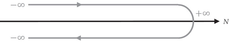
Figure 1: Closed-time-path $C$ of integration used in the “in-in” formalism.

To avoid the formal path integral along the closed contour $C$, one can divide it in two path integrals over the forward ($+$) and backwards ($-$) parts of the time contour $C=C^{+}\cup C^{-}$. This boils down to doubling the number of degrees of freedom in the path integral, with $\phi^{XI\pm}$ living respectively on $C^{+}$ and $C^{-}$. The $\pm$ fields and momenta should be considered independent, except at future infinity where the time path closes (truly, at any time later than the ones of interest), and where we use the usual boundary conditions that $\pm$ fields coincide, i.e. $\phi^{I+}(+\infty)=\phi^{I-}(+\infty)$, but that momenta $\pi_{I}^{\pm}$ are left unconstrained. The time flow being reversed on the $C^{-}$ branch, the path integral to perform can be rewritten along a forward contour only as

$$Z\left[J_{XI}^{\pm}\right]=\int_{C^{+}}\mathscr{D}\phi^{XI\pm}\exp\left(iS\left[\phi^{XI+}\right]-iS\left[\phi^{XI-}\right]+i\int\mathrm{d}^{4}xJ_{XI}^{+}\phi^{XI+}-i\int\mathrm{d}^{4}xJ_{XI}^{-}\phi^{XI-}\right).$$ (74)

In practice, we will make use of the so-called Keldysh basis (letting aside the various indices here):

$$\begin{pmatrix}\phi^{\mathrm{cl}}\\ \phi^{\mathrm{q}}\end{pmatrix}=\begin{pmatrix}1/2&1/2\\ 1&-1\end{pmatrix}\begin{pmatrix}\phi^{+}\\ \phi^{-}\end{pmatrix}\quad\Leftrightarrow\quad\begin{pmatrix}\phi^{+}\\ \phi^{-}\end{pmatrix}=\underbrace{\begin{pmatrix}1&1/2\\ 1&-1/2\end{pmatrix}}_{\textstyle K}\begin{pmatrix}\phi^{\mathrm{cl}}\\ \phi^{\mathrm{q}}\end{pmatrix},$$ (75)

where $\phi^{\mathrm{cl}}$ and $\phi^{\mathrm{q}}$ are respectively referred to as the classical and quantum components of the fields, and $K$ is the matrix of change of basis. The rationale for this denomination is that among the solutions of the saddle point equations for the Keldysh action $S\left[\phi^{XI+}\right]-S\left[\phi^{XI-}\right]$, there is always one with vanishing quantum component and classical component obeying the classical equation of motion $\delta S/\delta\phi^{XI}=0$. Although we are using natural units with $\hbar=1$, one can intuitively think of the quantum component as $\hbar$-suppressed, and indeed the stochastic equations we will derive, with classical equations of motion corrected by noises of quantum-mechanical origin, can be seen as semi-classical equations of motion.

Introducing covariant notations, latin indices $a$, $b$, $\cdots$ for the $\pm$ fields, and Fraktur indices $\mathfrak{a}$, $\mathfrak{b}$, $\cdots$ for the Keldysh label $\mathrm{cl}/\mathrm{q}$, the corresponding change of basis can be summarised as $\phi^{a}=K^{a}{}_{\mathfrak{a}}\phi^{\mathfrak{a}}$. To keep compact expressions, we use the convention of summation over repeated indices, and we will use well-chosen metrics to raise and lower them: the metric $\sigma_{3}{}_{ab}=\mathrm{diag}(1,-1)_{ab}$ in the $\pm$ basis; and the corresponding one $\sigma_{1}{}_{\mathfrak{a}\mathfrak{b}}=\left(\begin{smallmatrix}0&1\\ 1&0\end{smallmatrix}\right)_{\mathfrak{a}\mathfrak{b}}$ in the Keldysh basis. Note that in the latter, the matching condition of the CTP branches at future infinity reads $\phi^{I\mathrm{q}}(+\infty)=0$, again with no constraint on momenta. The generating functional in this basis reads (note that the Jacobian $|K|$ is unity)

$$Z\left[J_{XI}^{\mathfrak{a}}\right] =\int\mathscr{D}\phi^{XI\mathfrak{a}}\exp\left(iS\left[\phi^{XI\mathfrak{a}}\right]+i\int\mathrm{d}^{4}xJ_{XI}^{\mathrm{q}}\phi^{XI\mathrm{cl}}+i\int\mathrm{d}^{4}xJ_{XI}^{\mathrm{cl}}\phi^{XI\mathrm{q}}\right),$$ (76)

where $S\left[\phi^{XI\mathfrak{a}}\right]=S\left[\phi^{XI\mathrm{cl}}+\phi^{XI\mathrm{q}}/2\right]-S\left[\phi^{XI\mathrm{cl}}-\phi^{XI\mathrm{q}}/2\right]$.

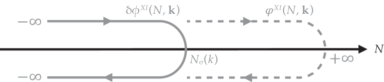
Figure 2: In the stochastic approach, the original path integral along the closed contour $C$ shown in Fig. 1 is divided for each wavenumber $\mathbf{k}$ into a path integral over UV fields $\delta\phi^{XI}(N,\mathbf{k})$, and into one over IR fields $\varphi^{XI}(N,\mathbf{k})$. Hence, the corresponding UV path is closed at the transition time $N_{\sigma}(k)$ with the boundary condition $\delta\phi^{I\mathrm{q}}(N_{\sigma}(k),\mathbf{k})=0$ (82), while the IR path starts there with the other boundary condition $\varphi^{I\mathrm{cl}}(N_{\sigma}(k),\mathbf{k})=0$, and is closed at future infinity with the boundary condition $\varphi^{I\mathrm{q}}(+\infty)=0$.

Formally, the “in-in” vacuum expectation value of any operator at time $t_{\star}$ can be computed by introducing this operator at this particular time on the closed-time-path of integration and with vanishing currents. Equivalently, $n$-point functions can be derived by calculating the $n^{\mathrm{th}}$ functional derivatives of the above generating functional $Z\left[J_{XI}^{\mathfrak{a}}\right]$ with respect to the external currents $J_{XI}^{\mathfrak{a}}$ and evaluating them at $J_{XI}^{\mathfrak{a}}=0$. As for the equations of motion verified by the expectation values of $\phi^{XI}$, they can be determined by extremising the quantum effective action, defined as the Legendre transformation of $W\left[J_{XI}^{\mathfrak{a}}\right]=-i\ln Z\left[J_{XI}^{\mathfrak{a}}\right]$. However in the following we choose to follow another route: based on the physical distinction between quantum short-wavelength modes and classical long-wavelength ones, we want to derive a classical (albeit stochastic) effective theory for the latter only, and then compute expectation values within this new theory. This amounts in our setup to derive what can be called the “coarse-grained effective Hamiltonian action” that governs the dynamics of the coarse-grained scalar fields in a Hamiltonian language (see e.g. Refs. Calzetta:1999zr ; Calzetta:2008iqa ; Vacca:2012vt for related concepts). Indeed, based on the scale separation provided by the physical Hubble radius $H^{-1}$, the original fields can be written in real space as IR+UV: $\phi^{XI\mathfrak{a}}(x)=\varphi^{XI\mathfrak{a}}(x)+\delta\phi^{XI\mathfrak{a}}(x)$, where we have in mind the Fourier cutoff $k_{\sigma}(N)$ discussed in Sec. 2. The Fourier components of the fields and momenta thus verify:

$$\phi^{XI\mathfrak{a}}\left(N,\mathbf{k}\right)=\left\{\begin{array}[]{ll}\delta\phi^{XI\mathfrak{a}}\left(N,\mathbf{k}\right),&\text{ if }N<N_{\sigma}(k),\\ \varphi^{XI\mathfrak{a}}\left(N,\mathbf{k}\right),&\text{ if }N>N_{\sigma}(k),\end{array}\right.$$ (79)

where $N_{\sigma}(k)$ represents the time at which the modes of modulus $k$ cross the UV/IR cutoff, and hence at which boundary conditions need to be specified for the fields. Because the UV modes $\delta\phi^{\mathfrak{a}}(N,\mathbf{k})$ stop being defined at the time $N_{\sigma}(k)$, their time path actually closes at this particular time, which enforces the boundary condition $\delta\phi^{I\mathrm{q}}\left(N_{\sigma}(k),\mathbf{k}\right)=0$, like for the full fields whose time path closes at future infinity. Inversely, the time path of IR modes $\varphi^{\mathfrak{a}}(N,\mathbf{k})$ begins at that time, with vanishing initial conditions for the classical component of the fields, $\varphi^{I\mathrm{cl}}\left(N_{\sigma}(k),\mathbf{k}\right)=0$ (see Fig. 2). Note that again, neither IR nor UV momenta are constrained at the time $N_{\sigma}(k)$.

Because these conditions will be crucial to specify interactions between IR and UV modes, we rewrite them together:

$$\phi^{I\mathfrak{a}}\left(N_{\sigma}(k),\mathbf{k}\right)=\left\{\begin{array}[]{ll}\delta\phi^{I\mathrm{cl}}\left(N_{\sigma}(k),\mathbf{k}\right),&\text{ if }\mathfrak{a}=\mathrm{cl},\\ \varphi^{I\mathrm{q}}\left(N_{\sigma}(k),\mathbf{k}\right),&\text{ if }\mathfrak{a}=\mathrm{q},\end{array}\right.$$ (82)

assigning the Fourier component at the transition time, either fully to the UV part for the classical component, or fully to the IR part for the quantum component. It will become clear when discussing IR-UV interactions in the discretised version of the path integral that, indeed, no boundary condition is required for the momenta, because in the path integral they can be evaluated at intermediate time steps and we can avoid to specify their values at the exact time $N_{\sigma}(k)$. It was actually shown in the context of a single test scalar field in de Sitter that these boundary conditions at $N_{\sigma}(k)$ enables the to-be-found stochastic description to correctly reproduce the propagators of the corresponding free QFT Tokuda:2017fdh ; Tokuda:2018eqs . Now that this decomposition into IR and UV fields is fully specified, one may rewrite the generating functional (at vanishing currents for simplicity) as

$$Z =\int\mathscr{D}\varphi^{XI\mathfrak{a}}\exp\left(iS_{\mathrm{eff}}\left[\varphi^{XI\mathfrak{a}}\right]\right),\qquad\text{with}$$ (83)

$$\exp\left(iS_{\mathrm{eff}}\left[\varphi^{XI\mathfrak{a}}\right]\right) =\int\mathscr{D}\delta\phi^{XI\mathfrak{a}}\exp\left(iS\left[\varphi^{XI\mathfrak{a}}+\delta\phi^{XI\mathfrak{a}}\right]\right),$$ (84)

where the path integral over the UV modes has to be performed explicitly. Then, we will see that upon the introduction of auxiliary stochastic variables describing possible deviations from the classical EoM, one needs not perform the path integral over the IR fields, but simply observe which IR trajectories have non-zero weights in the remaining path integral, and hence obtain the desired Langevin equations. However before that, let us note that Eq. (84) provides only a “naive” expression, and that one has to be careful about the fact that field perturbations themselves do not transform covariantly under field redefinitions beyond linear order Vilkovisky:1984st ; Gong:2011uw . To ensure that the resulting effective theory respects general covariance, the path integral should be expressed in terms of covariant objects, and we now turn to the identifications of suitable ones in our Hamiltonian formulation.

4.2 Covariant perturbations in the Hamiltonian language

It is well known that field perturbations are not covariant objects beyond linear order. This subtlety is usually irrelevant if one is only interested in the Gaussian properties of the inflationary fluctuations, because SPT is defined around homogeneous fields ${\phi_{0}}^{XI}(N)$ that solve the classical equations of motion, $\frac{\delta S}{\delta\phi^{XI}}\big{\rvert}_{{\phi_{0}}^{XI}}=0$, and any non-covariant contribution coming from the linear action in terms of $\delta\phi^{XI}$ thus vanishes. However, the aim of stochastic inflation is precisely to take into account the difference between the effective equations of motion verified by the coarse-grained scalar fields and the classical equations of motion verified by ${\phi_{0}}^{XI}(N)$ in SPT. In this context, the part of the action that is linear in $\delta\phi^{XI}$ not only does not vanish but actually plays a crucial role. Thus, in stochastic inflation, perturbations should be covariant objects at least up to quadratic order, even to describe only Gaussian statistics and contrary to SPT.

In anticipation of our later setup, we define the perturbations at some spacetime point $x$ by the displacements of the full inflaton fields $\phi^{I}(x)$ and their conjugate momenta $\pi_{I}(x)$ from their coarse-grained values $\varphi^{I}(x)$ and $\varpi_{I}(x)$ (the homogeneous background ${\phi_{0}}$ and ${\pi_{0}}$ would instead be used as reference fields in SPT):

$$\delta\phi^{I}(x)=\phi^{I}(x)-\varphi^{I}(x),\qquad\delta\pi_{I}(x)=\pi_{I}(x)-\varpi_{I}(x).$$ (85)

These finite displacements (85) do not transform covariantly under field redefinitions beyond the linear approximation, and therefore one needs to relate them to contravariant/covariant infinitesimal perturbations. The $\delta\phi$’s expansion has been already discussed in Ref. Gong:2011uw . The two neighbouring points in field space $\phi(x)$ and $\varphi(x)$ can be connected by a unique field-space geodesic, which we parameterise by the affine parameter $\lambda$ such that $\phi(\lambda=0)=\varphi(x)$ and $\phi(\lambda=1)=\phi(x)$ (see Fig. 3). We then define the Vilkovisky-DeWitt-type variable $Q^{I}$ by the “initial velocity”

$$\left.\frac{\mathrm{d}\phi^{I}}{\mathrm{d}\lambda}\right|_{\lambda=0}=Q^{I}.$$ (86)

This geometrical definition ensures that $Q^{I}$ lies in the tangent space of the point $\varphi(x)$, i.e. that it behaves as desired as a vector under field redefinitions. Using the fact that, by definition, $\phi^{I}(\lambda)$ verifies the geodesic equation

$${\cal D}_{\lambda}^{2}\phi^{I}(\lambda)=\frac{\mathrm{d}^{2}\phi^{I}}{\mathrm{d}\lambda^{2}}+\Gamma^{I}_{JK}\frac{\mathrm{d}\phi^{J}}{\mathrm{d}\lambda}\frac{\mathrm{d}\phi^{K}}{\mathrm{d}\lambda}=0\,,$$ (87)

where ${\cal D}_{\lambda}$ represents the covariant derivative with respect to the affine parameter $\lambda$, one can express $\phi^{I}(\lambda)$ in terms of $Q^{I}$ by using the following expansion around $\lambda=0$:

$$\phi^{I}(\lambda) =\phi^{I}(\lambda=0)+\left.\frac{\mathrm{d}\phi^{I}}{\mathrm{d}\lambda}\right|_{\lambda=0}\lambda+\frac{1}{2}\left.\frac{\mathrm{d}^{2}\phi^{I}}{\mathrm{d}\lambda^{2}}\right|_{\lambda=0}\lambda^{2}+\cdots$$

$$=\varphi^{I}+Q^{I}\lambda-\frac{1}{2}\Gamma^{I}_{JK}Q^{J}Q^{K}\lambda^{2}+\cdots,$$ (88)

thus obtaining the field perturbations

$$\delta\phi^{I}=\phi^{I}(\lambda=1)-\phi^{I}(\lambda=0)=Q^{I}-\frac{1}{2}\Gamma^{I}_{JK}Q^{J}Q^{K}+\cdots.$$ (89)

The non-tensorial feature of the Christoffel symbols explicitly shows the non-covariance of the finite perturbations $\delta\phi^{I}$ beyond the linear approximation.

The displacement $\delta\pi_{I}$ can also be expressed in terms of a truly covariant tensor in a similar way. For that, let us consider a family $\pi_{I}(\lambda)$ of covectors at each point along the geodesic $\phi^{I}(\lambda)$, and such that $\pi_{I}(\lambda=0)=\varpi_{I}(x)$ and $\pi_{I}(\lambda=1)=\pi_{I}(x)$. It is then natural to define a second Vilkovisky-DeWitt-type variable ${\tilde{P}}_{I}$ by the “initial momentum velocity” along the geodesic as

$${\tilde{P}}_{I}={\cal D}_{\lambda}\pi_{I}|_{\lambda=0}=\left(\frac{\mathrm{d}\pi_{I}}{\mathrm{d}\lambda}-\Gamma_{IJ}^{K}\pi_{K}\frac{\mathrm{d}\phi^{J}}{\mathrm{d}\lambda}\right)|_{\lambda=0}=P_{I}-\Gamma^{K}_{IJ}\varpi_{K}Q^{J},$$ (90)

where on the right-hand side, the naive $P_{I}$ such that $\delta\pi_{I}=\pi_{I}(\lambda=1)-\pi_{I}(\lambda=0)=P_{I}\lambda+{\cal O}(\lambda^{2})$ does not even transform covariantly at linear order, contrary to ${\tilde{P}}_{I}$, whose intrinsic geometrical definition ensures that it transforms as a covector at all order in perturbation theory. If one now imposes that the covectors ${\cal D}_{\lambda}\pi_{I}$ are parallel-transported along the geodesic:

$$0={\cal D}_{\lambda}^{2}\pi_{I}=\frac{\mathrm{d}^{2}\pi_{I}}{\mathrm{d}\lambda^{2}}-2\Gamma^{K}_{IJ}\frac{\mathrm{d}\phi^{J}}{\mathrm{d}\lambda}\frac{\mathrm{d}\pi_{K}}{\mathrm{d}\lambda}-(\Gamma^{S}_{IJ,K}-\Gamma^{S}_{IR}\Gamma^{R}_{JK}-\Gamma^{R}_{IJ}\Gamma^{S}_{RK})\pi_{S}\frac{\mathrm{d}\phi^{J}}{\mathrm{d}\lambda}\frac{\mathrm{d}\phi^{K}}{\mathrm{d}\lambda},$$ (91)

it is possible to express $\delta\pi_{I}$ in terms of ${\tilde{P}}_{I}$. However, we note that imposing ${\cal D}_{\lambda}^{2}\pi_{I}=0$ is one simple possible choice, but that others are possible, corresponding to a freedom in the identification of a suitable covariant momentum perturbation. We refer the interested reader to Appendix B for more details on this point, to which we will come back, and here just quote the relation between $\delta\pi_{I}$ and ${\tilde{P}}_{I}$ for this particular choice:

$$\delta\pi_{I}={\tilde{P}}_{I}+\Gamma^{K}_{IJ}\varpi_{K}Q^{J}+\Gamma^{K}_{IJ}Q^{J}{\tilde{P}}_{K}+\frac{1}{2}(\Gamma^{S}_{IJ,K}-\Gamma^{S}_{IR}\Gamma^{R}_{JK}+\Gamma^{R}_{IJ}\Gamma^{S}_{RK})\varpi_{S}Q^{J}Q^{K}+\cdots.$$ (92)

Equipped with these geometrically defined objects, we are now ready to compute the covariant effective action up to second order in the UV fields and momenta as

$$\exp\left(iS_{\mathrm{eff}}[\varphi^{XI\mathfrak{a}}]\right)=\int\mathscr{D}Q^{\tilde{X}I\mathfrak{a}}\exp\left(iS^{(0)}[\varphi^{XI\mathfrak{a}}]+S^{(1)}[\varphi^{XI\mathfrak{a}},Q^{\tilde{X}I\mathfrak{a}}]+S^{(2)}[\varphi^{XI\mathfrak{a}},Q^{\tilde{X}I\mathfrak{a}}]\right),$$ (93)

with $Q^{\tilde{X}I\mathfrak{a}}=(Q^{I\mathfrak{a}},{\tilde{P}}^{I\mathfrak{a}})$ used as a short-hand notation, and like for Eq. (73), $\mathscr{D}Q^{\tilde{X}I\mathfrak{a}}$ truly refers to the canonical phase-space measure $\prod_{I,\mathfrak{a},J,\mathfrak{b}}\mathscr{D}Q^{I\mathfrak{a}}\mathscr{D}{\tilde{P}}_{J}^{\mathfrak{b}}$.

4.3 Covariant CTP action and IR-UV interactions

To investigate the effect of linear UV perturbations on the IR dynamics, we must first covariantly expand the action up to second order in the perturbations. Starting from the Hamiltonian action (12), and expanding it up to second order in the fields’ covariant UV perturbations $Q^{\tilde{X}I}$ as well as metric UV perturbations $\mathcal{N}_{\text{UV}}$ and $\psi$, one finds

$$S^{(0)} =\int\mathrm{d}^{4}x\,a^{3}\left[\varpi_{I}\varphi^{I\prime}-\frac{1}{H}\left(\frac{1}{2}G^{IJ}\varpi_{I}\varpi_{J}+V+3M_{\text{Pl}}^{2}H^{2}\right)\right],$$ (94)

$$S^{(1)} =\int\mathrm{d}^{4}x\,a^{3}\left[{\tilde{P}}_{I}\left(\varphi^{I\prime}-\frac{\varpi^{I}}{H}\right)-Q^{I}\left({\cal D}_{N}\varpi_{I}+3\varpi_{I}+\frac{V_{I}}{H}\right)-\mathcal{N}_{\text{UV}}\left(\frac{1}{2}\varpi_{I}\varpi^{I}+V-3M_{\text{Pl}}^{2}H^{2}\right)\right],$$ (95)

$$S^{(2)} =\int\mathrm{d}^{4}x\,a^{3}\left[-3M_{\text{Pl}}^{2}H^{3}\mathcal{N}_{\text{UV}}^{2}-\mathcal{N}_{\text{UV}}\left(\varpi_{I}{\tilde{P}}^{I}+V_{I}Q^{I}+2M_{\text{Pl}}^{2}H^{2}\frac{\partial_{i}^{2}}{a^{2}}\psi\right)+\varpi_{I}Q^{I}\frac{\partial_{i}^{2}}{a^{2}}\psi\right.$$

$$\qquad\left.-\frac{1}{H}\left(\frac{1}{2}{\tilde{P}}_{I}{\tilde{P}}^{I}-\frac{1}{2}Q_{I}\frac{\partial_{i}^{2}}{a^{2}}Q^{I}+\frac{1}{2}V_{;IJ}Q^{I}Q^{J}-\frac{1}{2}R_{I}{}^{JK}{}_{L}\varpi_{J}\varpi_{K}Q^{I}Q^{L}\right)+{\tilde{P}}_{I}{\cal D}_{N}Q^{I}\right.$$

$$\qquad\left.+\left(\varphi^{I\prime}-\frac{\varpi^{I}}{H}\right)\frac{1}{2}R_{IJK}{}^{L}\varpi_{L}Q^{J}Q^{K}\right]\,.$$ (96)

In usual perturbation theory, where the coarse-grained fields and momenta are replaced by their homogeneous values that are solutions of the classical equations of motion dictated by $S^{(0)}$, the linear action $S^{(1)}$ vanishes. It is thus sufficient to use covariant variables at linear order only, and one needs not bother about quadratic terms in $(Q^{I},{\tilde{P}}_{I})$ in Eqs. (89) and (92). Here on the contrary, $S^{(1)}$ does not vanish because the time derivatives of the coarse-grained fields and momenta differ slightly from their classical values (by a quantity one can interpret as a classical random noise as we shall find soon). Relatedly, one can check that the manifest covariance of the result (94)–(96) would not have hold if one had not expanded $\delta\phi^{XI}$ to quadratic order in covariant perturbations. Let us now examine its three contributions.

Pure IR sector

$S^{(0)}$ governs the propagation and self-interactions of the IR fields, without consideration of the UV modes at all. More generally, it should be interpreted as dictating the deterministic drift for the IR fields. Notice that in general, for generic potential $V$ and field-space metric $G_{IJ}$, this classical drift action can be non-linear in the IR modes. Thus, we will not bother writing explicitly a rather complex expression for $S^{(0)}\left[\varphi^{XI\mathfrak{a}}\right]=S^{(0)}[\varphi^{XI\mathrm{cl}}+\varphi^{XI\mathrm{q}}/2]-S^{(0)}[\varphi^{XI\mathrm{cl}}-\varphi^{XI\mathrm{q}}/2]$, given that we will only be interested in its variation evaluated at classical IR solutions, which simply reads

$$\left.\frac{\delta S^{(0)}\left[\varphi^{XI\mathfrak{a}}\right]}{\delta\varphi^{YJ\mathrm{q}}}\right|_{\varphi^{YJ\mathrm{q}}=0}=\left.\frac{\delta S^{(0)}\left[\varphi^{XI}\right]}{\delta\varphi^{YJ}}\right|_{\varphi^{XI}=\varphi^{XI\mathrm{cl}}}.$$ (97)

In a related manner, one can see that because of its structure, $S^{(0)}\left[\varphi^{XI\mathfrak{a}}\right]$ only contains odd powers of $\varphi^{XI\mathrm{q}}$, the quantum component of the fields. Thus, its expansion in quantum fields is trivial up to quadratic order, and one can actually write:

$$S^{(0)}\left[\varphi^{XI\mathfrak{a}}\right]=\left.\int\mathrm{d}^{4}x\frac{\delta S^{(0)}\left[\varphi^{XI}\right]}{\delta\varphi^{YJ}(x)}\right|_{\varphi^{XI}=\varphi^{XI\mathrm{cl}}}\varphi^{YJ\mathrm{q}}(x)+\mathcal{O}\left(\varphi^{\mathrm{q}}\right)^{3}\,.$$ (98)

IR-UV interactions

As already stated, we focus in this derivation on the IR-UV interactions stemming from the continuous flow of quantum UV modes to the open system of classical IR ones, which results from the time-dependent Fourier cutoff $k_{\sigma}(N)$. Interestingly, these interactions are encoded in $S^{(1)}$ in the time derivatives of the IR fields, as seen in the heuristic approach (Sec. 2). We thus focus on those terms and neglect other ones in $S^{(1)}$, which amounts to considering the time derivatives acting as $\delta(N-N_{\sigma}(k))$ in Fourier space as we shall see now.

However first, because we will write the discretised version of the linear action $S^{(1)}$, it will prove useful to take a step back. The form of $S^{(1)}$ that we displayed in Eq. (95) is physically appealing because it makes explicitly appear the background EoM for the IR fields, times the UV perturbations, in an explicitly covariant form. However to find it we had first to integrate by parts the term $\int\mathrm{d}^{4}xa^{3}Q^{I\prime}\varpi_{I}=-\int\mathrm{d}^{4}xa^{3}Q^{I}(\varpi_{I}^{\prime}+3\varpi_{I})$ and then combine it with the change from $P_{I}$ to ${\tilde{P}}_{I}=P_{I}-\Gamma^{K}_{IJ}\varpi_{K}Q^{J}$ to form the covariant time derivative ${\cal D}_{N}\varpi_{I}$. Thus, going back to this previous version, the relevant terms in $S^{(1)}$ can be more simply expressed (i.e. with less time derivatives) as $S^{(1)}\supset\int\mathrm{d}^{4}x\,a^{3}\left({\tilde{P}}_{I}\varphi^{I\prime}-Q^{I}({\cal D}_{N}\varpi_{I}+3\varpi_{I})\right)=\int\mathrm{d}^{4}x\,a^{3}\left(P_{I}\varphi^{I\prime}+Q^{I\prime}\varpi_{I}\right)$, which we will now take as our starting point to compute IR-UV interactions in the Keldysh basis. Note that each of these two terms is not covariant when taken separately, but that their sum is indeed covariant. Understanding why these terms with time derivatives are peculiar is easier in Fourier space, and requires the investigation of the action in terms of Keldysh fields:

$$S^{(1)}\left[\varphi^{XI\mathfrak{a}},Q^{XI\mathfrak{a}}\right]$$

$$\quad\supset\int\mathrm{d}N\frac{\mathrm{d}^{3}\mathbf{k}}{(2\pi)^{3}}\,a^{3}(N)\left[P_{I}^{\mathrm{cl}}\left(N,\mathbf{k}\right)\varphi^{I\mathrm{q}\prime}\left(N,\mathbf{k}\right)+Q^{I\mathrm{cl}\prime}\left(N,\mathbf{k}\right)\varpi_{I}^{\mathrm{q}}\left(N,\mathbf{k}\right)\right]+\left(\mathrm{cl}\leftrightarrow\mathrm{q}\right).$$ (99)

Now, remember that the same Fourier component of UV and IR modes can never be defined at the same time, except at the transition time $N_{\sigma}(k)$. Of course it means that the support of these terms is of measure zero, and this is actually why terms without derivatives were neglected in $S^{(1)}$. However the terms with derivatives that we kept play a special role. Let us look for example at the first term, going back to the discrete description of the phase-space path integral for the mode $\mathbf{k}$ around the time $N_{\sigma}(k)$:

$$\int_{N_{\sigma}(k)-\Delta N}^{N_{\sigma}(k)+\Delta N}\mathrm{d}N\,a^{3}(N)P_{I}^{\mathrm{cl}}\left(N,\mathbf{k}\right)\varphi^{I\mathrm{q}\prime}\left(N,\mathbf{k}\right)$$

$$\qquad=\Delta N\left[a^{3}(N_{\sigma}(k)+\widetilde{\Delta N})P_{I}^{\mathrm{cl}}\left(N_{\sigma}(k)+\widetilde{\Delta N},\mathbf{k}\right)\frac{\varphi^{I\mathrm{q}}\left(N_{\sigma}(k)+\Delta N,\mathbf{k}\right)-\varphi^{I\mathrm{q}}\left(N_{\sigma}(k),\mathbf{k}\right)}{\Delta N}\right.$$

$$\qquad\qquad\left.+a^{3}(N_{\sigma}(k)-\Delta N+\widetilde{\Delta N})P_{I}^{\mathrm{cl}}\left(N_{\sigma}(k)-\Delta N+\widetilde{\Delta N},\mathbf{k}\right)\frac{\varphi^{I\mathrm{q}}\left(N_{\sigma}(k),\mathbf{k}\right)-\varphi^{I\mathrm{q}}\left(N_{\sigma}(k)-\Delta N,\mathbf{k}\right)}{\Delta N}\right]$$

$$\qquad=a^{3}(N_{\sigma}(k)-\Delta N+\widetilde{\Delta N})\,P_{I}^{\mathrm{cl}}\left(N_{\sigma}(k)-\Delta N+\widetilde{\Delta N},\mathbf{k}\right)\varphi^{I\mathrm{q}}\left(N_{\sigma}(k),\mathbf{k}\right),$$ (100)

with $0<\widetilde{\Delta N}<\Delta N$ and where we used the conditions (79) to get the second equality. Note that while the fields’ values $\varphi^{I}$ and $Q^{I}$ are evaluated on the discrete time grid at $N_{j}=j\Delta N$, the momenta $\varpi_{I}$ and $P_{I}$ can be evaluated at intermediate time steps $\widetilde{N_{j}}=j\Delta N+\widetilde{\Delta N}$, which enables us to compute IR-UV interactions without specifying boundary conditions at the exact time $N_{\sigma}(k)$ for them. In the same way, we find that the second term contributes $-a^{3}(N_{\sigma}(k)+\widetilde{\Delta N})\,Q^{I\mathrm{cl}}\left(N_{\sigma}(k),\mathbf{k}\right)\varpi_{I}^{\mathrm{q}}\left(N_{\sigma}(k)+\widetilde{\Delta N},\mathbf{k}\right)$. As for the third and the fourth term from the $(\mathrm{cl}$-$\mathrm{q})$ permutation in Eq. (4.3), they vanish by virtue of the boundary conditions (82). Thus, the interaction action that we consider can be rewritten in the continuous limit as

$$S^{(\mathrm{int})}\left[\varphi^{XI\mathfrak{a}},Q^{XI\mathfrak{a}}\right] =\int\mathrm{d}^{4}x\int\frac{\mathrm{d}^{3}\mathbf{k}}{(2\pi)^{3}}\delta(N-N_{\sigma}(k))\mathrm{e}^{i\mathbf{k}\cdot\mathbf{x}}a^{3}\left[P_{I}(x)^{\mathrm{cl}}{\varphi}^{I\mathrm{q}}(N,\mathbf{k})-Q^{I\mathrm{cl}}(x)\varpi_{I}^{\mathrm{q}}(N,\mathbf{k})\right]$$

$$=\int\mathrm{d}^{4}x\,a^{3}Q^{XI\mathfrak{a}}(x)\varphi^{\prime}_{XI\mathfrak{a}}(x),$$ (101)

where we introduced the pseudo “time derivatives” $\varphi^{\prime}_{XI\mathfrak{a}}(x)$ with lower indices that are defined as

$$\begin{cases}\displaystyle\varphi^{\prime}_{QI\mathfrak{a}}(x):=-\delta^{\mathrm{cl}}_{\mathfrak{a}}\int\frac{\mathrm{d}^{3}\mathbf{k}}{(2\pi)^{3}}\delta(N-N_{\sigma}(k))\mathrm{e}^{i\mathbf{k}\cdot\mathbf{x}}\varpi_{I}{}^{\mathrm{q}}(N,\mathbf{k}),\\[10.0pt] \displaystyle\varphi^{\prime}_{PI\mathfrak{a}}(x):=\delta^{\mathrm{cl}}_{\mathfrak{a}}\int\frac{\mathrm{d}^{3}\mathbf{k}}{(2\pi)^{3}}\delta(N-N_{\sigma}(k))\mathrm{e}^{i\mathbf{k}\cdot\mathbf{x}}\varphi_{I}{}^{\mathrm{q}}(N,\mathbf{k}),\end{cases}$$ (102)

thus restricting the couplings to be of the form $\mathrm{UV}^{\mathrm{cl}}\times\mathrm{IR}^{\mathrm{q}}$. Those interaction terms will be the ones responsible for the modification of the classical equations of motion for the IR fields, once the UV perturbations are integrated out. Let us now investigate the dynamics of the latter.

UV dynamics

As a first comment, note that the last line of $S^{(2)}$ seemingly goes beyond the approximation of treating UV modes up to quadratic order in the action, as it consists of a quadratic term in the UV perturbations, multiplied by the “background-like” equation of motion for the IR fields, i.e. by a quantity of order of the to-be-found noise. The careful reader will also have noticed that such a term is exactly of the kind that can ambiguously appear depending on the exact definition of a covariant momentum UV perturbation ${\tilde{P}}_{I}$, as we explain in Appendix B. Because this arbitrariness can not affect the physics, we are free to make the choice ($\kappa=1/2$) such that this term proportional to the Riemann tensor of the field space vanishes. This procedure also fixes the form of $S^{(3)}$ as is shown in Appendix B, thus we conclude that this term does not affect the Gaussian properties of the theory and we will discard it in what follows, leaving for future work the investigation of this subtlety and of potentially interesting non-Gaussian features related to the geometry of the field space.

Extremising the action (94)–(96) with respect to the non-dynamical fields $\mathcal{N}_{\text{UV}}$ and $\psi$ that appear without any time-derivative, one recovers the local Friedmann equation (31) as well as the expressions (30) and (32) for $\mathcal{N}_{\text{UV}}$ and $\psi$ in terms of $Q^{I}$ and ${\tilde{P}}_{I}$. Plugging them back into the second-order action, one can write the latter in the condensed form

$$S^{(2)}=\frac{1}{2}\int\mathrm{d}^{4}x\mathrm{d}^{4}x^{\prime}Q^{XI}(x)\Lambda_{XYIJ}(x,x^{\prime})Q^{YJ}(x^{\prime}),$$ (103)

where we used the non-covariant variables $Q^{XI}$ that naturally appear in $S^{(\mathrm{int})}$ instead of the covariant perturbations $Q^{\tilde{X}I}$. As a result, some of the following intermediate steps will not be manifestly covariant. However, one is perfectly allowed to use such non-covariant objects to make calculations, and then to switch back to covariant ones using the relation (90) ${\tilde{P}}_{I}=P_{I}-\Gamma_{IJ}^{K}\varpi_{K}Q^{J}$. Instead of quoting the kernel $\Lambda_{XYIJ}$ corresponding to the non-covariant UV modes that only appear in intermediate steps, we rather show its covariant counterpart $\Lambda_{\tilde{X}\tilde{Y}IJ}$, which is given by

$$\begin{pmatrix}\Lambda_{QQIJ},&\Lambda_{Q{\tilde{P}}IJ}\\ \Lambda_{{\tilde{P}}QIJ},&\Lambda_{{\tilde{P}}{\tilde{P}}IJ}\end{pmatrix}=\delta^{(4)}(x-x^{\prime})a^{3}\begin{pmatrix}\frac{1}{H}\left(G_{IJ}\frac{\partial_{i}^{2}}{a^{2}}-M^{2}_{QQIJ}\right),&-G_{IJ}({\cal D}_{N}+3)-M^{2}_{Q{\tilde{P}}IJ}\\ G_{IJ}{\cal D}_{N}-M^{2}_{{\tilde{P}}QIJ},&-G_{IJ}/H\end{pmatrix},$$ (104)

where the differential operators act on the $x^{\prime}$ coordinates, and with $M^{2}_{QQIJ}$ and $M^{2}_{Q{\tilde{P}}IJ}=M^{2}_{{\tilde{P}}QIJ}$ already given in Eqs. (35)–(36).

Extremising $S^{(2)}$ with respect to the covariant UV perturbations yields the following classical EoM for the UV fields:

$$\int\mathrm{d}^{4}x^{\prime}\Lambda_{\tilde{X}\tilde{Y}IJ}(x,x^{\prime})Q^{\tilde{Y}J}(x^{\prime})=0,\quad\Leftrightarrow\quad\begin{cases}\displaystyle{\cal D}_{N}Q^{I}=\frac{{\tilde{P}}^{I}}{H}+M^{2}_{{\tilde{P}}Q}{}^{I}{}_{J}Q^{J},\\ \displaystyle{\cal D}_{N}{\tilde{P}}_{I}=-3{\tilde{P}}_{I}+\frac{1}{H}\left(G_{IJ}\frac{\partial_{i}^{2}}{a^{2}}-M^{2}_{QQIJ}\right)Q^{J}-M^{2}_{Q{\tilde{P}}I}{}^{J}{\tilde{P}}_{J}\,,\end{cases}$$ (105)

which are nothing else than equations (33) and (34) $E^{QI}=0=E^{{\tilde{P}}}_{I}$ found in the heuristic approach (Sec. 2). Strikingly, as we shall see in the next subsection, it is sufficient to know the (inverse of the) kernel operator $\Lambda$ to compute the corrections to the IR dynamics, due to their interactions with UV fluctuations as dictated by $S^{(\mathrm{int})}$. Thus, the UV modes dictating these corrections can be understood as evolving according to $S^{(2)}$ only, hence they verify the EoM (105), similar to the one of SPT but with background fields replaced by their infrared counterparts. This is an interesting improvement from the path-integral approach compared to the heuristic one, where we had to assume that the dynamics of UV modes was decoupled from the one of IR ones, see the paragraph before Eq. (25) and the one after Eq. (36).

Eventually, in the path integral (93) with doubled degrees of freedom, the quadratic action written in terms of the fields in the Keldysh basis reads:

$$S^{(2)}\left[\varphi^{XI\mathfrak{a}},Q^{XI\mathfrak{a}}\right]=\frac{1}{2}\int\mathrm{d}^{4}x\mathrm{d}^{4}x^{\prime}Q^{XI\mathfrak{a}}(x)\Lambda_{XYIJ\mathfrak{a}\mathfrak{b}}(x,x^{\prime})Q^{YJ\mathfrak{b}}(x^{\prime}),$$ (106)

where $\Lambda_{XYIJ\mathfrak{a}\mathfrak{b}}$ is given by the basis transformation $\Lambda_{XYIJ\mathfrak{a}\mathfrak{b}}=(K^{T})_{\mathfrak{a}}{}^{a}\Lambda_{XYIJab}K^{b}{}_{\mathfrak{b}}$, with $K$ given in Eq. (75), and with the $\pm$ basis operator

$$\Lambda_{XYIJab}=\mathrm{diag}\left(\Lambda_{XYIJ}(\varphi^{+}),-\Lambda_{XYIJ}(\varphi^{-})\right).$$ (107)

Note that, as the differential operator $\Lambda_{XYIJ}$ depends on the IR fields $\varphi^{XI}$, one has in principle to distinguish between its evaluations on $+$ IR fields and on $-$ IR fields: $\Lambda_{XYIJ}(\varphi^{+})$ and $\Lambda_{XYIJ}(\varphi^{-})$. However, as we already noticed, one can think of the expansion in the quantum components as an expansion in $\hbar$. In this respect, in order to derive the leading-order quantum effects, it sufficient to use the expression of $\Lambda$ at zeroth-order:

$$\Lambda_{XYIJab}=\Lambda_{XYIJ}(\varphi^{\mathrm{cl}})\sigma_{3ab}+\mathcal{O}\left(\varphi^{\mathrm{q}}\right)\delta_{ab}\,.$$ (108)

Although it may seem a crude approximation, we will check the consistency of this expansion in the next subsection, and explain why higher-order corrections are indeed not needed for our computation.

4.4 Covariant coarse-grained effective Hamiltonian action and Langevin equations

Now we have to gather the three contributions to the covariant coarse-grained Hamiltonian effective action and perform the following path integral:

$$\exp\left(iS_{\mathrm{eff}}[\varphi^{XI\mathfrak{a}}]\right)= \exp\left(iS^{(0)}[\varphi^{XI\mathfrak{a}}]\right)$$

$$\times\int\mathscr{D}Q^{XI\mathfrak{a}}\exp\left[i\int\mathrm{d}^{4}x\,a^{3}\varphi^{\prime}_{XI\mathfrak{a}}Q^{XI\mathfrak{a}}+\frac{i}{2}\int\mathrm{d}^{4}x\mathrm{d}^{4}x^{\prime}Q^{XI\mathfrak{a}}\Lambda_{XYIJ\mathfrak{a}\mathfrak{b}}Q^{YJ\mathfrak{b}}\right].$$ (109)

Note that we safely replaced the measure $\mathscr{D}Q^{\tilde{X}I\mathfrak{a}}$ by $\mathscr{D}Q^{XI\mathfrak{a}}$ in the path integral (93) as the Jacobian for the transformation $Q^{\tilde{X}I\mathfrak{a}}\to Q^{XI\mathfrak{a}}$ is exactly one. The Gaussian integral over the UV modes can be performed exactly to give:

$$S_{\mathrm{eff}}[\varphi^{XI\mathfrak{a}}]= \,S^{(0)}[\varphi^{XI\mathfrak{a}}]\underbrace{+\frac{i}{2}\ln\left[\mathrm{Det}\left(\Lambda\right)\right]}_{\textstyle\begin{array}[]{c}S_{\mathrm{ren}}[\varphi^{XI\mathrm{cl}}]\end{array}}\underbrace{-\frac{1}{2}\int\mathrm{d}^{4}x\mathrm{d}^{4}x^{\prime}\left(a^{3}\varphi_{XI\mathfrak{a}}^{\prime}\right)_{x}(\Lambda^{-1})^{XYIJ\mathfrak{a}\mathfrak{b}}{}_{xx^{\prime}}\left(a^{3}\varphi^{\prime}_{YJ\mathfrak{b}}\right)_{x^{\prime}}}_{\textstyle\begin{array}[]{c}S_{\mathrm{IA}}[\varphi^{XI\mathfrak{a}}]\end{array}}.$$ (112)

The first term dictates the classical, background dynamics of the IR fields, and contains no new information compared to SPT. The second term is nothing but the usual QFT one-loop correction which can be computed in principle, and then reabsorbed by renormalisations of the bare parameters in the classical action $S$. We will thus omit this contribution in the following, although the renormalisation procedure is of course highly non-trivial to perform explicitly. More important for us is the third contribution $S_{\mathrm{IA}}$ called the influence action, describing the influence on the coarse-grained fields of the small-scale UV fluctuations that were integrated out (or more generally, the influence of an environment on the system of interest Feynman:1963fq ). In the rest of this subsection, we compute this influence action, discuss its physical interpretation and derive the resulting stochastic equations for the coarse-grained fields.

As $\Lambda^{-1}$ is nothing but the closed-time-path-ordered two point correlation function of UV modes, it is easier to express it first in the $\pm$ basis with latin indices $a$, $b$, $\cdots$, and then translate it into the Keldysh basis with use of the matrix of change of basis $K^{a}{}_{\mathfrak{a}}$. So we first focus on

$$i(\Lambda^{-1} )^{XYIJab}(x,x^{\prime})$$

$$=\int\mathscr{D}Q^{XIa}\exp{\left[\frac{i}{2}\int\mathrm{d}^{4}x\mathrm{d}^{4}x^{\prime}Q^{XIa}\Lambda_{XYIJab}Q^{YJb}\right]}Q^{XIa}(x)Q^{YJb}(x^{\prime})$$ (113)

$$=\begin{cases}\displaystyle\theta(N-N^{\prime})\braket{\hat{Q}^{XI}(x)\hat{Q}^{YJ}(x^{\prime})}+\theta(N^{\prime}-N)\braket{\hat{Q}^{YJ}(x^{\prime})\hat{Q}^{XI}(x)},&(a=+,\,b=+),\\ \displaystyle\braket{\hat{Q}^{YJ}(x^{\prime})\hat{Q}^{XI}(x)},&(a=+,\,b=-),\\ \displaystyle\braket{\hat{Q}^{XI}(x)\hat{Q}^{YJ}(x^{\prime})},&(a=-,\,b=+),\\ \displaystyle\theta(N^{\prime}-N)\braket{\hat{Q}^{XI}(x)\hat{Q}^{YJ}(x^{\prime})}+\theta(N-N^{\prime})\braket{\hat{Q}^{YJ}(x^{\prime})\hat{Q}^{XI}(x)},&(a=-,\,b=-),\end{cases}$$

where the ordering of the quantum operators is determined by the chronological order along the closed-time path $C$, and the brackets $\braket{\cdots}$ denote usual vacuum expectation values of UV operators under the $\varphi^{XI}$-dependent measure $\mathscr{D}Q^{XI}\exp{\left(iS^{(2)}\left[\varphi^{XI},Q^{XI}\right]\right)}$. Note that these expectation values are unambiguously defined in the same way on both branches of the CTP, as we recall that for our computation, it is sufficient to evaluate the kernel $\Lambda$ with vanishing quantum components of the IR fields, i.e. $\Lambda(\varphi^{\mathrm{cl}})$, see Eq. (108). Thus, for each component of the $\Lambda^{-1}$ matrix we are able to forget the $\pm$ indices and we can compute them as in usual perturbation theory, but with background fields replaced by their IR counterparts.

With use of the dimensionless unequal time two-point functions

$$(2\pi)^{3}\delta^{(3)}(\mathbf{k}+\mathbf{k}^{\prime})\frac{2\pi^{2}}{k^{3}}\mathcal{P}^{XYIJ}(N,N^{\prime};k)=\Braket{\hat{Q}^{XI}(N,\mathbf{k})\hat{Q}^{YJ}(N^{\prime},\mathbf{k}^{\prime})},$$ (114)

$\Lambda^{-1}$ can be expressed more explicitly as

$$(\Lambda^{-1})^{XYIJab}(x,x^{\prime})$$

$$=-i\int\frac{\mathrm{d}^{3}\mathbf{k}}{(2\pi)^{3}}\mathrm{e}^{i\mathbf{k}\cdot(\mathbf{x}-\mathbf{x}^{\prime})}\frac{2\pi^{2}}{k^{3}}\begin{pmatrix}\begin{array}[]{c}\theta(N-N^{\prime})\mathcal{P}^{XYIJ}(N,N^{\prime};k)\\ +\theta(N^{\prime}-N){\mathcal{P}^{XYIJ}}^{*}(N,N^{\prime};k)\end{array}&{\mathcal{P}^{XYIJ}}^{*}(N,N^{\prime};k)\\ \mathcal{P}^{XYIJ}(N,N^{\prime};k)&\begin{array}[]{c}\theta(N^{\prime}-N)\mathcal{P}^{XYIJ}(N,N^{\prime};k)\\ +\theta(N-N^{\prime}){\mathcal{P}^{XYIJ}}^{*}(N,N^{\prime};k)\end{array}\end{pmatrix}^{ab},$$ (115)

where we used that $\mathcal{P}^{YXJI}(N^{\prime},N;k)={\mathcal{P}^{XYIJ}}^{*}(N,N^{\prime};k)$ as a consequence of $\hat{Q}^{XI}(x)$ being hermitian operators, and hence $\hat{Q}^{XI\dagger}(N,\mathbf{k})=\hat{Q}^{XI}(N,-\mathbf{k})$. We now express $\Lambda^{-1}$ in the Keldysh basis as

$$(\Lambda^{-1})^{XYIJ}{}_{\mathfrak{a}\mathfrak{b}}(x,x^{\prime})=(K^{T})_{\mathfrak{a}}{}^{a}\sigma_{3ab}\,(\Lambda^{-1})^{XYIJbc}(x,x^{\prime})\,\sigma_{3cd}K^{d}{}_{\mathfrak{b}}$$

$$=-i\int\frac{\mathrm{d}^{3}\mathbf{k}}{(2\pi)^{3}}\mathrm{e}^{i\mathbf{k}\cdot(\mathbf{x}-\mathbf{x}^{\prime})}\frac{2\pi^{2}}{k^{3}}\begin{pmatrix}0&-2i\theta(N^{\prime}-N)\mathrm{Im}\mathcal{P}^{XYIJ}(N,N^{\prime};k)\\ 2i\theta(N-N^{\prime})\mathrm{Im}\mathcal{P}^{XYIJ}(N,N^{\prime};k)&\mathrm{Re}\mathcal{P}^{XYIJ}(N,N^{\prime};k)\end{pmatrix}_{\mathfrak{a}\mathfrak{b}}\,,$$ (116)

where we used $\theta(N^{\prime}-N)+\theta(N-N^{\prime})=1$. The influence action $S_{\mathrm{IA}}$ in Eq. (112) can then be explicitly obtained after contracting twice with $\varphi^{\prime}_{XI}{}^{\mathfrak{a}}(x)\propto\delta^{\mathfrak{a}}_{\mathrm{q}}\delta(N-N_{\sigma}(k))$ (note that the position of the $\mathfrak{a}$ index has been flipped compared to Eq. (102) with use of the $\sigma_{1}^{\mathfrak{a}\mathfrak{b}}$ metric), retaining only the $\mathrm{q}$-$\mathrm{q}$ component of Eq. (4.4) evaluated at equal times $N=N^{\prime}=N_{\sigma}(k)$:

$$S_{\mathrm{IA}}= \,\frac{i}{2}\int\mathrm{d}^{4}x\mathrm{d}^{4}x^{\prime}\left(a^{3}\varphi_{XI}{}^{\mathrm{q}}\right)_{x}(\mathrm{Re}\Pi^{XYIJ})_{xx\prime}\left(a^{3}\varphi_{YJ}{}^{\mathrm{q}}\right)_{x^{\prime}},$$ (117)

where

$$\Pi^{XYIJ}(x,x^{\prime}) =\int\frac{\mathrm{d}^{3}\mathbf{k}}{(2\pi)^{3}}\mathrm{e}^{i\mathbf{k}\cdot(\mathbf{x}-\mathbf{x}^{\prime})}\frac{2\pi^{2}}{k^{3}}\delta(N-N_{\sigma})\delta(N^{\prime}-N_{\sigma})\mathcal{P}^{XYIJ}(N,N^{\prime};k)$$

$$=\frac{k_{\sigma}{}^{\prime}}{k_{\sigma}}\frac{\sin\left(k_{\sigma}|\mathbf{x}-\mathbf{x}^{\prime}|\right)}{k_{\sigma}|\mathbf{x}-\mathbf{x}^{\prime}|}\mathcal{P}^{XYIJ}(N,k_{\sigma})\delta(N-N^{\prime}),$$ (118)

with $\mathcal{P}$ on the second line being simply the usual equal-time dimensionless two-point correlation function. Note that any higher-order correction in the quantum components of the IR fields, coming from evaluating $\Lambda$ beyond the leading order result (108), would generate terms of order $\mathcal{O}(\varphi^{\mathrm{q}})^{3}$ in the influence action. Put it otherwise, our computation is exact up to quadratic order in the quantum components.

Although we have just seen that the contractions with the “time derivatives” $\varphi^{\prime}_{XI}{}^{\mathfrak{a}}$ only kept the information about the $\mathrm{q}$-$\mathrm{q}$ component of $\Lambda^{-1}{}_{\mathfrak{a}\mathfrak{b}}$, it is still interesting to notice the “causality structure” 2009AdPhy..58..197K ; Calzetta:2008iqa of this operator.

Classical-Classical component.

First, the “cl-cl” component in Eq. (117) is zero. It is also easy to check that there is no term independent of $\varphi^{\mathrm{q}}$ in the fully nonlinear, purely IR Keldysh action $S^{(0)}[\varphi^{XI\mathrm{cl}},\varphi^{XI\mathrm{q}}]$, as can be seen for example from its expansion (98) in the quantum components of the IR fields. This means that for vanishing quantum components $\varphi^{XI\mathrm{q}}=0$, the effective action $S_{\mathrm{eff}}=S^{(0)}+S_{\mathrm{IA}}$ is zero: $S_{\mathrm{eff}}[\varphi^{XI\mathrm{cl}},0]=0$. This was expected because for $\varphi^{\mathrm{q}}=0$, the fields coincide on the forward and backward parts of the closed-time contour and thus the two contributions cancel each other. A last interpretation is that the quantum components do not propagate alone and must mix to classical ones. In this respect, note that although our derivation was done at lowest non-trivial order in the quantum components of the fields and momenta, with $\Lambda\to\Lambda(\varphi^{\mathrm{cl}})$ in the path integral over UV modes, this property actually holds non-perturbatively. Indeed, any correction to the current computation would be proportional to powers of $\varphi^{\mathrm{q}}$, and thus would still be vanishing when evaluated on configurations with purely classical components.

Classical-Quantum component.

This component is interesting because, although non-zero in Eq. (4.4), it results in a vanishing contribution to the influence action after contracting with the “time-derivatives” $\varphi^{\prime}_{XI}{}^{\mathfrak{a}}\propto\delta^{\mathfrak{a}}_{\mathrm{q}}$, a property inherited from the boundary conditions (82). If $\varphi^{I\mathrm{cl}}$ and $Q^{I\mathrm{q}}$ were not vanishing at $N_{\sigma}(k)$, $S_{\mathrm{IA}}$ would be augmented by a cross-term of the form $\left[\varphi^{\mathrm{cl}}\left(\Lambda^{-1}\right)_{\mathrm{cl},\mathrm{q}}\varphi^{\mathrm{q}}+\left(\mathrm{cl}\leftrightarrow\mathrm{q}\right)\right]$ and proportional to the imaginary part of the power spectrum. The mixed “q-cl”/“cl-q” components in the influence action are more generally known for describing the dissipation of the system (the IR modes) by backreacting on the environment (the UV modes), and being responsible for the famous fluctuation-dissipation theorem. Indeed, if no boundary condition was imposed at the time $N_{\sigma}(k)$, the classical field configurations $\varphi_{XI}{}^{\mathrm{cl}}(x)$ would get an extra friction term in their equations of motion of the form $-2\int\mathrm{d}^{4}x^{\prime}\,\mathrm{Im}\Pi^{XYIJ}(x,x^{\prime})a^{3}(N^{\prime})\varphi_{YJ}{}^{\mathrm{cl}}(x^{\prime})$. However in our setup of stochastic inflation, the continuous flow from UV to IR modes via the time-dependent cutoff $k_{\sigma}(N)$ is unidirectional and we expect no such backreaction, and thus no dissipation.

Quantum-Quantum component.

The “q-q” component is the only one that survives in the influence action after contracting with the pseudo “time-derivatives”, and because it is quadratic in the quantum parts of the fields and momenta, it constitutes a non-trivial quantum correction to the classical dynamics, again describing the effects of the integrated out short-scale fluctuations on the IR sector. Let us now discuss its physical implications.

Strikingly, the influence action (117) is purely imaginary. This implies that in the path integral (83) over the IR components, the weights of configurations with non-zero quantum components are exponentially suppressed. This important fact warrants that our expansion in the quantum components of the fields (and momenta) is well justified. In a related manner, even though we do not use the formalism of density matrices in our paper, it can be shown quite generally that such imaginary “$\mathrm{q}$-$\mathrm{q}$” component in the influence action acts to suppress the off-diagonal terms of the reduced density matrix $\rho_{\mathrm{r}}(\varphi^{+},\varphi^{-})$ obtained after tracing out the environment (the UV modes here), a process that can be understood as decoherence (see, e.g. Refs. Feynman:1963fq ; Calzetta:2008iqa ). The exponential suppression of the quantum components of the fields in the weigth $\mathrm{e}^{iS_{\mathrm{IA}}}$ of the path integral is of course reminiscent of statistical field theory. Following the seminal paper of Feynman and Vernon Feynman:1963fq , this insight is put to good use by performing what is sometimes called a Hubbard-Stratonovich transformation 1957SPhD….2..416S ; 1959PhRvL…3…77H : introducing auxiliary fields $\xi^{XI}$, the exponential of the influence action can be rewritten as

$$\mathrm{e}^{iS_{\mathrm{IA}}}=\int\mathscr{D}\xi^{XI}P\left[\xi^{XI};\varphi^{XI\mathrm{cl}}\right]\mathrm{e}^{i\int\mathrm{d}^{4}x\,a^{3}\xi^{XI}\varphi_{XI}{}^{\mathrm{q}}},$$ (119)

where $P\left[\xi^{XI};\varphi^{XI\mathrm{cl}}\right]$ denotes the Gaussian weight

$$P[\xi^{XI};\varphi^{XI\mathrm{cl}}]=\sqrt{\mathrm{Det}(2\pi\mathrm{Re}\Pi)}^{-1}\exp\left[-\frac{1}{2}\int\mathrm{d}^{4}x\mathrm{d}^{4}x^{\prime}\xi^{XI}\left(\mathrm{Re}\Pi^{-1}_{XYIJ}\right)_{\varphi^{XI\mathrm{cl}}}\xi^{YJ}\right]\,,$$ (120)

and where the subscript $\varphi^{XI\mathrm{cl}}$ recalls that $\Pi$, as essentially the Green’s function of $\Lambda(\varphi^{XI\mathrm{cl}})$, can thus be seen as a (complicated) functional of the IR classical components $\varphi^{XI\mathrm{cl}}$. The manipulation (119)–(120) is a simple mathematical identity, in essence the inverse of a Gaussian integration. Yet, it offers a very useful physical insight. Indeed, the partition function (83) can now be rewritten as

$$Z =\int\mathscr{D}\varphi^{XI\mathfrak{a}}\exp\left(iS_{\mathrm{eff}}[\varphi^{XI\mathfrak{a}}]\right)\,$$ (121)

$$=\int\mathscr{D}\varphi^{XI\mathrm{cl}}\int\mathscr{D}\xi^{XI}P\left[\xi^{XI};\varphi^{XI\mathrm{cl}}\right]\int\mathscr{D}\varphi^{XI\mathrm{q}}\,\mathrm{exp}(\underbrace{iS^{(0)}\left[\varphi^{XI\mathfrak{a}}\right]+i\int\mathrm{d}^{4}x\,a^{3}\xi^{XI}\varphi_{XI}{}^{\mathrm{q}}}_{\textstyle\begin{array}[]{c}i\tilde{S}_{\mathrm{eff}}[\varphi^{XI\mathfrak{a}},\xi^{XI}]\end{array}})\,,$$ (123)

with $\int\mathscr{D}\xi^{XI}P[\xi^{XI};\varphi^{XI\mathrm{cl}}]=1$ for any realisation of $\varphi^{XI\mathrm{cl}}$. Upon the introduction of the Hubbard-Stratonovich fields $\xi^{XI}$, the imaginary quadratic interactions of the quantum components in $S_{\mathrm{eff}}[\varphi^{XI\mathfrak{a}}]$ have been turned into a real linear coupling between the quantum components and the auxiliary fields in the new real effective action $\tilde{S}_{\mathrm{eff}}[\varphi^{XI\mathfrak{a}},\xi^{XI}]$. Of course, the physical interpretation behind Eq. (121) is that $P\left[\xi^{XI};\varphi^{XI\mathrm{cl}}\right]$ endows the $\xi$’s with Gaussian statistics with

$$\begin{cases}\displaystyle\braket{\xi^{XI}(x)}\equiv\int\mathscr{D}\xi^{XI}\xi^{XI}(x)P\left[\xi^{XI};\varphi^{XI\mathrm{cl}}\right]=0,\\ \displaystyle\braket{\xi^{XI}(x)\xi^{YJ}(x^{\prime})}\equiv\int\mathscr{D}\xi^{XI}\xi^{XI}(x)\xi^{YJ}(x^{\prime})P\left[\xi^{XI};\varphi^{XI\mathrm{cl}}\right]=\left.\mathrm{Re}\,\Pi^{XYIJ}(x,x^{\prime})\right|_{\varphi^{XI\mathrm{cl}}}.\end{cases}$$ (124)

The delta function $\delta(N-N^{\prime})$ in $\mathrm{Re}\Pi$, see Eq. (4.4), indicates that $\xi$’s can be interpreted as Gaussian white noises, like in the heuristic approach, with amplitudes determined by the power spectra of the UV modes on the “background” of the IR classical components. Additionally, it is interesting to notice that the reality of the noise is guaranteed in this first-principle derivation, contrary to the heuristic approach where this feature has to be added by hand (see Sec. 2.5). The partition function (121) together with equations (4.4) and (124) represent one of the main results of this paper.

It is now relatively straightforward to take into account the effect of the quantum components on the classical ones. Indeed, recall that our computation of $S_{\mathrm{eff}}[\varphi^{XI\mathfrak{a}}]$ was made up to quadratic order in the quantum components. Consistently neglecting cubic terms in the expression (98) for $S^{(0)}$, the quantum components therefore enter only linearly in $\tilde{S}_{\mathrm{eff}}[\varphi^{XI\mathfrak{a}},\xi^{XI}]$, and the path integral over them can hence be performed explicitly, yielding the delta functional $\delta\left(\left.\frac{\delta S^{(0)}\left[\varphi^{XI}\right]}{\delta\varphi_{YJ}}\right|_{\varphi^{XI}=\varphi^{XI\mathrm{cl}}}+a^{3}\xi^{YJ}\right)$ in the remaining path integral over the classical components of the IR fields, $\varphi^{\mathrm{cl}}$, and the auxiliary variables $\xi$. Thus, the only trajectories with non-zero weights in the path integral are the ones that verify the following equations of motion:

$$\varphi^{I\mathrm{cl}}{}^{\prime}=\frac{\varpi^{I\mathrm{cl}}}{H}+\xi^{QI},\qquad\varpi_{I}^{\mathrm{cl}}{}^{\prime}=-3\varpi_{I}^{\mathrm{cl}}-\frac{V_{I}\left(\varphi^{I\mathrm{cl}}\right)}{H}+\frac{1}{H}\Gamma^{K}_{IJ}\left(\varphi^{I\mathrm{cl}}\right)\varpi_{K}^{\mathrm{cl}}\varpi^{J\mathrm{cl}}+\xi^{P}_{I},$$ (125)

where we will omit to write explicitly “cl” for simplicity in what follows. While the first equation is already in a manifestly covariant form, the second one is not. However this is not surprising as neither $\varpi_{I}^{\prime}$ nor $P_{I}$ (that was integrated out), are covariant quantities themselves. However this equation does respect general covariance, as is seen by using $\xi^{P}_{I}=\xi^{{\tilde{P}}}_{I}+\Gamma^{K}_{IJ}\varpi_{K}\xi^{QJ}$, as well as $\varpi_{I}^{\prime}={\cal D}_{N}\varpi_{I}+\Gamma^{K}_{IJ}\varpi_{K}\varphi^{J\prime}$ and replacing $\varphi^{J\prime}$ by its value according to the first Langevin equation. Eventually, the stochastic EoM (125) can be summarised in an explicitly covariant way as (again, removing the “cl” exponent for conciseness)

$$\varphi^{I\prime}=\frac{\varpi^{I}}{H}+\xi^{QI},\qquad{\cal D}_{N}\varpi_{I}=-3\varpi_{I}-\frac{V_{I}}{H}+\xi^{{\tilde{P}}}_{I}.$$ (126)

As we discussed at length in Sec. 3, these Langevin equations should be understood as the continuous limit of a discrete process with a Stratonovich scheme. Moreover, the identification of independent quantum fields in the Bunch-Davies regime provides one, upon classicalisation, with an essentially unique set of independent white noises with which to formulate these Stratonovich Langevin-type equations. As we also explained there, Itô’s discretisation also has a number of advantages, and one can convert the latter equations into the corresponding Itô’s ones as:

$$\boxed{\mathfrak{D}_{N}\varphi^{I}=\frac{\varpi^{I}}{H}+\xi^{QI},\qquad\mathfrak{D}_{N}\varpi_{I}=-3\varpi_{I}-\frac{V_{I}}{H}+\xi^{\tilde{P}}_{I},}$$ (127)

with use of the Itô-covariant derivatives (43)–(45). Let us also remind the reader that the local Hubble parameter $H$ is explicitly given in terms of the IR fields and momenta through the Friedmann constraint (31)

$$3M_{\text{Pl}}^{2}H^{2}=\frac{1}{2}G^{IJ}(\varphi)\varpi_{I}\varpi_{J}+V(\varphi)\,,$$ (128)

without modification compared to the heuristic approach.

Eventually, let us comment on the status of these equations. As the derivation above shows, these are the semi-classical equations governing the trajectories that have a non-zero weight in the closed-time path integral, but they do not yet correspond to physical quantities: the expectation values of the quantum theory are only recovered once taking the ensemble averages over the noises. More precisely, this statistical average exactly reproduces the quantum average only when the initial effective action $S_{\mathrm{eff}}[\varphi^{XI\mathfrak{a}}]$ is at most quadratic in the quantum components, resulting in the above delta functional (letting aside here the fact that we only integrated out the UV fluctuations at quadratic order in the action). It is in that sense that the stochastic equations (127), derived at lowest non-trivial order in the quantum components, can be qualified as “semi-classical”.

As described in Sec. 3, physical quantities derived from Itô’s SDE (127) only depend on the auto-correlation of the noises, which is physically specified by the UV two-point correlations. The presence of Itô-covariant derivatives also manifestly guarantees general covariance. These equations are thus free from any stochastic anomaly. Furthermore, as we stressed above, the reality of noises is also ensured, as their auto-correlations (124) derived from the CTP formalism are automatically given by the real part of the UV two-point functions.

5 Markovian analytical approximations and phase-space Fokker-Planck equation

As we explained in Sec. 2.6, stochastic inflation is strictly speaking not described by a Markov process. Indeed, the noise amplitude is the solution of the differential equation verified by the UV modes which develop on the stochastic IR background, rather than an explicit function of the IR fields themselves. In particular, the noise amplitude a priori depends on the whole past history of the stochastic process. However, in some situations, the noise amplitude can be approximately expressed in terms of the instantaneous IR fields, in which case the dynamics can be thought of as Markovian and a powerful tool becomes accessible: the Fokker-Planck equation. In this section, we deal with these Markovian cases. We begin by showing the covariant Fokker-Planck equation that dictates the evolution of the one-point probability density function (PDF) for the IR fields and momenta, that can be inferred from the Langevin equations (127) when assuming a Markovian dynamics. Then we show how to approximate the noise amplitude, first in the simpler situation in which the scalar fields are strictly massless, and then in a generic case under the assumption of slow-varying masses.

5.1 Covariant Fokker-Planck equation in phase space

Let us first reemphasise that throughout this work, we treat the fields as locally homogeneous, i.e. at leading order in a gradient expansion. Although this might seem very crude, following the separate universe approach, this nonetheless enables one to capture the full nonlinear dynamics on super-Hubble scales. Hence, as described in Sec. 2.3, the Langevin equations (127) govern the stochastic dynamics of a representative $\sigma$-Hubble patch. In the Markovian limit, with the assumption that the noise amplitudes are well approximated as functions of the current IR field values (and momenta), these Langevin equations give rise to the corresponding Fokker-Planck (FP) equation, with use of the rule presented in Appendix A.3, as

$$\partial_{N}P= -D_{\varphi^{I}}\left[\frac{G^{IJ}}{H}\varpi_{J}P\right]+\partial_{\varpi_{I}}\left[\left(3\varpi_{I}+\frac{V_{I}}{H}\right)P\right]$$

$$+\frac{1}{2}D_{\varphi^{I}}D_{\varphi^{J}}(A^{QQIJ}P)+D_{\varphi^{I}}\partial_{\varpi_{J}}(A^{Q{\tilde{P}}I}{}_{J}P)+\frac{1}{2}\partial_{\varpi_{I}}\partial_{\varpi_{J}}(A^{{\tilde{P}}{\tilde{P}}}{}_{IJ}P)\,.$$ (129)

Here we defined a last covariant derivative $D_{\varphi^{I}}$ with respect to the IR fields, the phase-space one, whose action on a rank-1 tensor is $D_{\varphi^{I}}\mathcal{U}^{J}=\nabla_{I}\mathcal{U}^{J}+\Gamma_{IL}^{K}\varpi_{K}\partial_{\varpi_{L}}\mathcal{U}^{J}$ and generalisation to rank-$n$ tensors is straightforward. As for the $A^{\tilde{X}\tilde{Y}IJ}$’s, these are the noises’ auto-correlations at coincident points:

$$A^{\tilde{X}\tilde{Y}IJ}(N)\delta(N-N^{\prime})=\braket{\xi^{\tilde{X}I}(N)\xi^{\tilde{Y}J}(N^{\prime})}=\frac{k_{\sigma}^{\prime}}{k_{\sigma}}\mathrm{Re}[\mathcal{P}^{\tilde{X}\tilde{Y}IJ}(N,k_{\sigma}(N))]\delta(N-N^{\prime}),$$ (130)

which are here assumed to be functions of $\varphi^{I}(N)$ and $\varpi_{I}(N)$, and up to the factor $k_{\sigma}^{\prime}/k_{\sigma}$ that may be approximated by unity, are nothing else than the real parts of the UV power spectra.

One should remember that in the FP equation in field space (41), which we previously wrote for pedagogical reasons, the scalar PDF $P_{\mathrm{s}}$ is rescaled compared to the PDF $P$ that directly results from the Langevin equations. Here, on the contrary, it is easy to check that the phase-space PDF $P(\varphi^{I},\varpi_{I},N)$ (truly the transition probability given some initial state), is already a scalar quantity, without the need of any rescaling. In this respect, although we skipped the intermediate steps of the computation, we stress that Eq. (5.1) is not postulated, but simply derived from the Langevin equations and Eq. (171), with covariant phase-space derivatives naturally emerging from the computation. Given the important complexity of the phase-space Itô-Langevin equations (127), the manifestly covariant form of the FP equation (5.1) is rather remarkable and provides a non-trivial consistency check of the former. This equation generalises the FP equation that we proposed in our previous paper in a simpler setup Pinol:2018euk : in field space and for test scalar fields in de Sitter spacetime only. Also, the “stochastic anomalies” were not solved there, and the form of the FP equation was simply assumed based on the requirement of general covariance. Not only do we present here the derivation of this phase-space FP equation, but we are also confident that it can now be used to compute correlation functions of multifield inflation with curved field space in realistic setups where the fields backreact on the geometry of spacetime. However, it would be restrictive to consider that the virtue of this equation only concerns these situations: the Itô-Stratonovich ambiguity was also plaguing single-field inflation, and our first-principle derivation, with emphasis on manifest covariance, enabled us to solve it in this simpler context as well.

The remaining nontrivial difficulty is now to prescribe values for the auto-correlation of the noises $A^{\tilde{X}\tilde{Y}IJ}$, and in the next two sections, we turn to interesting particular cases where we can give analytical estimates. Note that this will be possible because we assume from now on a slow-varying regime, which was not the case until here. Also, because the dynamics of the UV modes in SPT is conveniently solved in terms of the conformal time $\tau$ such that $\mathrm{d}N=aH\mathrm{d}\tau$, we will also make use of this time variable in what follows. In our context in which $H$ is a stochastic quantity, conformal time is strictly speaking not a deterministic variable like the number of $e$-folds, but we will nonetheless make this approximation, justified as follows. The noise auto-correlation at time $N$ only depends on the UV fluctuations with wavenumber $k_{\sigma}(N)$, which exited the Hubble radius $\simeq-\mathrm{ln}(\sigma)$ $e$-folds before $N$. As the UV fluctuations follow the Bunch-Davies behaviour until only a few $e$-folds before Hubble crossing (all the more so for light fields of particular relevance in the stochastic formalism), in practice it is necessary to follow the evolution of a given mode $k_{\sigma}(N)$ during only for a few $e$-folds (typically 5), a duration that is not large enough for stochastic effects to accumulate and significantly affect the local Hubble scale.

5.2 Massless limit

For analytically understanding the UV fluctuations, it is particularly useful to use the projections of the mode functions on a set of parallel-transported vielbeins, the $Q^{\alpha}_{A}$ introduced in Eq. (65). They provide independent degrees of freedom deep inside the Hubble radius, only mixing via the projected mass matrix $M^{2}{}^{\alpha}{}_{\beta}$, as can be seen from their EoM (66). In this section, we consider that this projected mass matrix is completely negligible. By consistency of the slow-varying approximation, we also use the zeroth-order, locally de-Sitter expression of the scale factor $a(\tau)\simeq-1/(H_{\star}\tau)$, where $H_{\star}$ denotes the Hubble scale, considered constant around Hubble crossing, i.e. in the period interpolating between the Bunch-Davies regime and the crossing of the coarse-graining scale, such that $k_{\sigma}(\tau)\tau\simeq-\sigma(1+{\cal O}(\epsilon))$.

Under these conditions, the mode functions $Q^{\alpha}_{A}$ simply provide $N_{\mathrm{fields}}$ independent copies $\left(Q^{\alpha}_{A}\propto\delta^{\alpha}_{A}\right)$ of the standard single-field massless mode function in quasi de Sitter spacetime, which read, with Bunch-Davies initial condition:

$$Q^{\alpha}_{A}(\tau,k)=-i\delta^{\alpha}_{A}\frac{\mathrm{e}^{-ik\tau}}{a\sqrt{2k}}\left(1-\frac{i}{k\tau}\right)\,.$$ (131)

Note that we used the freedom of redefining mode functions with an arbitrary unitary matrix as explained in Sec. 3.2, in order to choose a phase that leads to explicitly real values of $Q^{\alpha}_{A}$ (and ${\tilde{P}}^{\alpha}_{A}$) on super-Hubble scales. From these mode functions, and using Eq. (54), one deduces the multifield power spectrum of the UV modes at coarse-graining scale crossing:

$$\mathcal{P}^{QQIJ}\left(\tau,k_{\sigma}(\tau)\right) =\frac{k_{\sigma}(\tau)^{3}}{2\pi^{2}}e^{I}_{\alpha}e^{J}_{\beta}Q^{\alpha}_{A}\left(\tau,k_{\sigma}(\tau)\right)Q^{\beta*}_{A}\left(\tau,k_{\sigma}(\tau)\right)$$

$$=\left(\frac{H_{\star}}{2\pi}\right)^{2}G^{IJ}\left(1+\sigma^{2}\right),$$ (132)

where we recall that $\sigma\ll 1$, so that the last term should be neglected. Notice that although mass effects are not taken into account in this section, the introduction of the parallel-transported vielbeins enables one to capture the geometrical effects of the curved field space at the level of UV fields $\left(\mathcal{P}^{QQIJ}\propto G^{IJ}\right)$. Then, neglecting slow-roll suppressed metric perturbations $\propto M^{2}{}_{{\tilde{P}}Q}$ in ${\tilde{P}}$ for consistency, the momentum UV modes read

$${\tilde{P}}^{\alpha}_{A}(\tau,k) \simeq\frac{\mathrm{d}}{a\mathrm{d}\tau}Q^{\alpha}_{A}(\tau,k)=-\delta^{\alpha}_{A}\frac{H^{2}\mathrm{e}^{-ik\tau}}{\sqrt{2k^{3}}}k^{2}\tau^{2}\,,$$ (133)

so that using again Eq. (54), one obtains, for the power spectra involving momenta :

$$\mathcal{P}^{Q{\tilde{P}}I}{}_{J}\left(\tau,k_{\sigma}(\tau)\right) =-\sigma^{2}H_{\star}\left(\frac{H_{\star}}{2\pi}\right)^{2}\delta^{I}_{J}\left(1-i\sigma\right),$$ (134)

$$\mathcal{P}^{{\tilde{P}}{\tilde{P}}}{}_{IJ}\left(\tau,k_{\sigma}(\tau)\right) =\sigma^{4}H_{\star}^{2}\left(\frac{H_{\star}}{2\pi}\right)^{2}G_{IJ}\,.$$ (135)

Note that the cross power-spectrum has a non-zero imaginary part $\mathrm{Im}\mathcal{P}^{Q{\tilde{P}}I}{}_{J}=\sigma^{3}H_{\star}\left(\frac{H_{\star}}{2\pi}\right)^{2}\delta^{I}_{J}$, remnant from the quantum nature of the scalar fields, and completely fixed by the non-vanishing commutation relation between $Q$ and ${\tilde{P}}$ in Eq. (50). Naturally, the fact that it is suppressed by the small parameter $\sigma$ is related to the highly squeezed state of the fluctuations and to the fact that they “classicalise” on super-Hubble scales. However, notice anyway that the Schwinger-Keldysh derivation shows that only the real parts of the power spectra appear in the statistics of the stochastic noises.

In the strict massless and “slow-roll” regime of this section, the mode functions of the momenta (133) at coarse-graining scale crossing are suppressed by $\sigma^{2}$ compared to the ones of the fields (131), hence the power spectra involving the former should be self-consistently set to zero in practical computations. However, this property only holds within this framework, and in general, the power spectra involving momenta, while “slow-roll” suppressed, are not $\sigma$ suppressed and should be considered, as we will show in the next section.

5.3 Slow-varying masses

Let us now go one step further and consider the effects of a non-zero mass matrix $M^{2}{}^{\alpha}{}_{\beta}$. First we notice that at early times the mass term is negligible compared to the gradient term, i.e., $\forall\alpha,\beta,\quad M^{2}{}^{\alpha}{}_{\beta}\ll k^{2}/a^{2}$. Thus initial conditions and the first stage of evolution of the perturbations are equivalent to the massless case. However, the behaviour is different around Hubble crossing. To identify these non-trivial mass effects, we make the assumption that the projected mass matrix is approximately constant in the period interpolating between the Bunch-Davies regime and the crossing of the coarse-graining scale, a feature observed in many concrete models of inflation. It is then possible to diagonalise the mass matrix locally, around the time of Hubble crossing, making use of the set of mass eigenvalues $m_{i}^{2}$ and corresponding eigenvectors $D^{\alpha}{}_{i}$ such that $M^{2\alpha}{}_{\beta}D^{\beta}{}_{i}=m_{i}^{2}D^{\alpha}{}_{i}$  (no sum on $i$). According to our assumption, these quantities can be considered constant in the interpolating period, so that the vielbein-basis EoM (66) result then in the simple set of diagonal equations in the mass eigenbasis:

$$\partial_{N}^{2}Q^{i}_{A}+\left(3-\epsilon\right)\partial_{N}Q^{i}_{A}+\left(\frac{k^{2}}{a^{2}H^{2}}+\frac{m^{2}_{i}}{H^{2}}\right)Q^{i}_{A}=0,\qquad\text{(no sum on $i$)},$$ (136)

where $Q^{i}_{A}=(D^{-1})^{i}{}_{\alpha}Q^{\alpha}_{A}$ denotes the projected mode functions on the mass eigenbasis. We here note that the mass matrix $M^{2\alpha}{}_{\beta}$ is real and symmetric, hence the mass eigenvalue $m_{i}^{2}$ are real, and one can take the diagonalising matrix $D^{\alpha}{}_{i}$ to be a real orthonormal matrix (with $(D^{-1})^{i}{}_{\alpha}=(D^{T})^{i}{}_{\alpha}=D^{\alpha}{}_{i}$). It is important to notice that the mass eigenvalues $m_{i}^{2}$ are scalars in field space, and that they also correspond to eigenvalues of the original mass matrix $M^{2}{}^{I}{}_{J}$, with eigenvectors given by $e^{I}_{i}=e^{I}_{\alpha}D^{\alpha}{}_{i}$, i.e.

$$M^{2I}{}_{J}e^{J}_{i}=m_{i}^{2}e^{I}_{i},\qquad\text{(no sum on $i$)}.$$ (137)

Moreover, taking into account the orthonormality of $D^{\alpha}{}_{i}$, the set of vectors $e^{I}_{i}$, rotated from the vielbeins $e^{I}_{\alpha}$, constitute another set of vielbeins, hence satisfying $G_{IJ}e^{I}_{i}e^{J}_{j}=\delta_{ij}$ and $\delta^{ij}e^{I}_{i}e^{J}_{j}=G^{IJ}$.

The initial conditions for the $Q^{i}_{A}$ are simply given by $Q^{i}_{A}(\tau,k)\underset{-k\tau\gg 1}{\to}\frac{-i}{a\sqrt{2k}}(D^{-1})^{i}{}_{A}\mathrm{e}^{-ik\tau}$ with $(D^{-1})^{i}{}_{A}=(D^{-1})^{i}{}_{\alpha}\delta^{\alpha}_{A}$, so that the corresponding solution of Eq. (136) reads, at leading-order in the slow-varying approximation:

$$Q^{i}_{A}(\tau,k)=(D^{-1})^{i}{}_{A}Q^{i}(\tau,k),\qquad\text{(no sum on $i$)},$$ (138)

with $Q^{i}$ the familiar single-field mode function

$$Q^{i}(\tau,k)=\frac{\mathrm{e}^{i(\nu_{i}-1/2)\pi/2}}{2a}\sqrt{-\pi\tau}H_{\nu_{i}}^{(1)}(-k\tau),\quad\text{with }\nu_{i}=\begin{cases}\displaystyle\sqrt{\frac{9}{4}-\frac{m_{i}^{2}}{H^{2}}},&\text{if }\displaystyle\frac{m_{i}^{2}}{H^{2}}<\frac{9}{4},\\[10.0pt] \displaystyle i\sqrt{\frac{m_{i}^{2}}{H^{2}}-\frac{9}{4}},&\text{if }\displaystyle\frac{m_{i}^{2}}{H^{2}}\geq\frac{9}{4}.\end{cases}$$ (139)

expressed in terms of $H_{\nu_{i}}^{(1)}$, the Hankel function of the first kind and of order $\nu_{i}$. Hence, one obtains the dimensionless power spectrum of UV modes at the time when $k=\sigma aH$ as

$$\mathcal{P}^{QQIJ}(\tau,k_{\sigma}(\tau))=\frac{k_{\sigma}^{3}(\tau)}{2\pi^{2}}\sum_{i}e^{I}_{i}e^{J}_{i}|Q^{i}(\tau,k_{\sigma}(\tau))|^{2},$$ (140)

where we used the orthonormality of the matrix $D^{\alpha}{}_{i}$. The result (140) is interesting because intermediate steps like the parallel-transported vielbeins or the diagonalising matrix $D^{\alpha}{}_{i}$ disappear altogether: to compute the right-hand side, the only requirement is to know the mass eigenvalues $m^{2}_{i}$ and the corresponding eigenvectors $e^{I}_{i}$ forming a set of vielbeins, Eq. (137), which is easy to obtain numerically from $M^{2I}{}_{J}$ once a position in phase space $\left(\varphi^{I},\varpi_{I}\right)$ is specified. Moreover, the sum in Eq. (140) is nicely understood as a mass-weighted metric in field space, and indeed, the massless limit $\propto G^{IJ}$ is easily recovered by setting $\nu_{i}=3/2,\,\forall i$. Notice also that $\mathcal{P}^{QQIJ}$ is automatically real and symmetric, as should be from first principles (see Sec. 3.2).

Moving to momenta, and according to the UV EoM (105), one obtains

$${\tilde{P}}^{i}_{A}=H\partial_{N}Q^{i}_{A}-\frac{\varpi^{i}\varpi_{j}}{2M_{\text{Pl}}^{2}H}Q^{j}_{A},$$ (141)

where $\varpi_{i}=e^{I}_{i}\varpi_{I}$. Using the properties of Hankel functions, we note that the time derivative of $Q^{i}$ can be simply expressed, at leading-order in the slow-varying approximation, as

$$\partial_{N}Q^{i}|_{k_{\sigma}}=q_{\nu_{i}}(\sigma)Q^{i}|_{k_{\sigma}},\quad\text{with}\quad q_{\nu_{i}}(\sigma)=\nu_{i}-\frac{3}{2}-\sigma\frac{H_{\nu_{i}-1}^{(1)}(\sigma)}{H_{\nu_{i}}^{(1)}(\sigma)}\,,$$ (142)

where we evaluated it at the time of crossing of the coarse-graining scale. One therefore obtains

$${\tilde{P}}^{i}_{A}|_{k_{\sigma}}=\sum_{j}\left(Hq_{\nu_{i}}(\sigma)\delta^{i}_{j}-\frac{\varpi^{i}\varpi_{j}}{2M_{\text{Pl}}^{2}H}\right)(D^{-1})^{j}{}_{A}Q^{j}|_{k_{\sigma}}\equiv\sum_{j}\mathscr{Q}^{i}{}_{j}(D^{-1})^{j}{}_{A}Q^{j}|_{k_{\sigma}},$$ (143)

so that all power spectra at coarse-graining scale crossing can be summarised as

$$\mathcal{P}^{QQIJ} =\frac{k_{\sigma}^{3}}{2\pi^{2}}\sum_{i}e^{I}_{i}e^{J}_{i}|Q^{i}|^{2}_{k_{\sigma}},$$ (144)

$$\mathcal{P}^{Q{\tilde{P}}I}{}_{J} =\frac{k_{\sigma}^{3}}{2\pi^{2}}\sum_{i,j}e^{I}_{i}e_{Jj}\mathscr{Q}^{*j}{}_{i}|Q^{i}|^{2}_{k_{\sigma}},$$ (145)

$$\mathcal{P}^{{\tilde{P}}{\tilde{P}}}{}_{IJ} =\frac{k_{\sigma}^{3}}{2\pi^{2}}\sum_{i,j,k}e_{Ii}e_{Jj}\mathscr{Q}^{i}{}_{k}\mathscr{Q}^{*j}{}_{k}|Q^{k}|^{2}_{k_{\sigma}}.$$ (146)

One knows from first principles that $\mathcal{P}^{{\tilde{P}}{\tilde{P}}}{}_{IJ}$ should be real and symmetric, similarly to $\mathcal{P}^{QQIJ}$, while $\mathrm{Im}\mathcal{P}^{Q{\tilde{P}}I}{}_{J}=\sigma^{3}H_{\star}\left(\frac{H_{\star}}{2\pi}\right)^{2}\delta^{I}_{J}$. Because our analytical expressions are based on several approximations, these properties are not necessarily precisely verified by Eqs. (145)–(146), a discrepancy that can be used as a quantitative diagnostic of the quality of the approximations in practical numerical computations. However, we note once again that only the real parts of the power spectra anyway enter into the properties of the stochastic noises (see Eq. (130)).

Although obtained for analytically estimating the noises amplitudes in stochastic multifield inflation, Eqs. (144)–(146) are of more general interest in the context of multifield inflation with slow-varying quantities, replacing $\sigma$ by $k/aH$ when necessary, and they constitute new results to the best of our knowledge. Given the number of approximations performed, it is difficult to control the degree of accuracy of the above formulae, but they constitute a proof of principle that it is possible to obtain Markovian analytical approximations, and they constitute a basis for future improvements.

The discussion has been kept quite general until now, but as is well known, the behaviour of super-Hubble fluctuations strongly depends on the mass parameter. Hence, from these generically applicable formulas, in the stochastic context, two physically different regimes should be distinguished depending on the various values of $m_{i}^{2}$, leading either to real positive $\nu_{i}$ for “light” fields (the first line in Eq. (139)), or imaginary $\nu_{i}\equiv i\mu_{i}$ for heavy fields (the second line there). For heavy fields, one can write

$$\frac{k_{\sigma}^{3}(\tau)}{2\pi^{2}}|Q^{i}(\tau,k_{\sigma}(\tau))|^{2}\underset{\frac{m_{i}^{2}}{H^{2}}\geq\frac{9}{4}}{=}4\pi\mathrm{e}^{-\mu_{i}\pi}\left(\frac{H}{2\pi}\right)^{2}\left(\frac{\sigma}{2}\right)^{3}|H_{i\mu_{i}}^{(1)}(\sigma)|^{2}\,,$$ (147)

with the small argument expansion

$$H_{i\mu}^{(1)}(\sigma)\underset{\sigma\ll 1}{\simeq}-i\frac{\Gamma(i\mu)}{\pi}\left(\frac{\sigma}{2}\right)^{-i\mu}+\frac{1+\coth(\mu\pi)}{\Gamma(1+i\mu)}\left(\frac{\sigma}{2}\right)^{i\mu}\,.$$ (148)

The factor $|H_{i\mu_{i}}^{(1)}(\sigma)|^{2}$ in Eq. (147) hence describes the characteristic super-Hubble oscillations of heavy fields, but more importantly here, the power spectrum (147) is suppressed by $\sigma^{3}$. This explicit dependence on the a priori arbitrary coarse-graining parameter $\sigma$ is not really worrisome: it simply comes from the fact that fluctuations of heavy fields are strongly suppressed on super-Hubble scales, and should simply be discarded from the stochastic description (and in the sums (145)–(146)), whose aim is to describe the long-term dynamics generated by light scalars. Turning to them, and using $H_{\nu}^{(1)}(\sigma)\underset{\sigma\ll 1}{\simeq}-(i/\pi)\Gamma(\nu)\left(\sigma/2\right)^{-\nu}$, the last term of $q_{\nu_{i}}(\sigma)$ in Eq. (142) should be neglected as of order $\sigma^{2}$, and one obtains

$$\frac{k_{\sigma}^{3}(\tau)}{2\pi^{2}}|Q^{i}(\tau,k_{\sigma}(\tau))|^{2}\underset{\frac{m_{i}^{2}}{H^{2}}<\frac{9}{4}}{=}\left(\frac{H}{2\pi}\right)^{2}\left(\frac{\Gamma(\nu_{i})}{\Gamma(3/2)}\right)^{2}\left(\frac{\sigma}{2}\right)^{3-2\nu_{i}}\,,$$ (149)

here with only a power-law dependence on $\sigma$. This dependence can be neglected, and $\left(\frac{\sigma}{2}\right)^{3-2\nu_{i}}$ can be approximated by unity, under the condition that the latter is taken to verify

$$\frac{\sigma}{2}\gg\mathrm{e}^{-\left(3-2\nu_{i}\right)^{-1}},$$ (150)

which is easily compatible with $\sigma\ll 1$ for a light enough mass (see Refs. Starobinsky:1994bd ; Grain:2017dqa for discussions in a single-field context). For intermediate masses $0.1\lesssim m_{i}^{2}/H^{2}\lesssim 1$, stochastic effects are less important but may not be completely negligible (see, e.g., Ref. Fumagalli:2019ohr ), and the resulting $\sigma$-dependence indicates that the coarse-graining procedure, made at leading-order in the gradient expansion, should be refined in order to properly treat these situations. More precisely, let us add that in theories that are not completely scale invariant, it is expected that the Langevin equations, which describe the distribution of field values in $\sigma$-Hubble patches, do depend on $\sigma$. Yet another question is to see how $\sigma$ disappears when computing physical observables on scales much larger than the cutoff scale. It is likely that the stochastic-$\delta N$ approach needs to be modified to deal with these situations of intermediate masses, but this is largely outside the scope of this paper.

Eventually, as discussed in Sec. 3.2, one can check explicitly that for light scalars with $m_{i}^{2}<9/4H^{2}$, the complex mode functions $Q^{I}_{A}(N,k)$ and ${\tilde{P}}_{IA}(N,k)$ (or equivalently, $Q^{i}_{A}$ and ${\tilde{P}}^{i}_{A}$) become approximately real up to an irrelevant constant unitary matrix. This stems from the fact that, the $Q^{\alpha}$ being independent fields inside the Hubble radius, the variables $(D^{-1})^{i}{}_{\alpha}Q^{\alpha}$, obtained by rotation of the former, equally provide a set of independent variables (and indeed, we have seen that the orthonormal matrix $D^{\alpha}{}_{i}$ drops out of all correlators). Hence, one could also have rotated the annihilation (and creation) operators $\hat{a}^{A}$ and absorbed in their definitions the individual phase factors $\mathrm{e}^{i\nu_{i}\pi/2}$ of the mode functions (139). The corresponding transformation can be described by the relations (48)–(49) with the unitary matrix

$$U^{{\bar{A}}}{}_{B}=D^{{\bar{A}}}{}_{i}\,\mathrm{diag}\left(\mathrm{e}^{i(\nu_{i}-3/2)\pi/2}\right){\!}^{i}{}_{j}(D^{-1})^{j}{}_{B}\,,$$ (151)

with which one obtains the expressions

$$\bar{Q}^{i}_{\bar{A}}=(D^{-1})^{i}{}_{\bar{A}}\mathrm{e}^{-i(\nu_{i}-3/2)\pi/2}Q^{i}\quad\text{(no sum on $i$)}\,,\qquad\bar{{\tilde{P}}}^{i}_{{\bar{A}}}=\mathscr{Q}^{i}{}_{j}\bar{Q}^{j}_{\bar{A}}$$ (152)

that become manifestly real on super-Hubble scales.

6 Conclusions

In this paper, we derive an effective stochastic theory for the super-Hubble, coarse-grained, scalar fields during inflation. We do so in a phase-space approach and for the general class of nonlinear sigma models (1), characterised by their potentials and curved field spaces. We first give in section 2 a “heuristic” derivation of the corresponding Langevin equations in phase space, in order to introduce concepts and notations used all the way. We point out the limitations of the heuristic approach that uses the classical equations of motion, as well as the non-Markovian nature of the dynamics. Section 3 is devoted to the resolution of the “inflationary stochastic anomalies” that we pointed out in our previous paper Pinol:2018euk : because of the very quantum nature of the scalar fields, the theory contains a preferred frame that corresponds to the basis of independent creation and annihilation operators. This frame must be used to define independent noises in the Langevin equations, removing the possibility of any ambiguity in the choice of such a frame, and the corresponding Langevin equations should be interpreted according to a Stratonovich, midpoint, discretisation scheme. Along this discussion, we show how the classicalisation of quantum fluctuations on super-Hubble scales enables one to interpret the noises as classical random variables rather than quantum operators. We also show explicitly the transformation of the Stratonovich-Langevin equations to their Itô version by the addition of noise-induced drifts, and explain how these terms can be combined with the usual time-derivatives to define new, covariant in Itô calculus, time-derivatives. With the final form (2), the Langevin equations can be readily used in numerical and analytical computations.

Section 4 is devoted to the rigorous derivation of the Langevin equations using a path-integral approach, which solves the remaining conceptual issues of the heuristic one. We begin by recalling that for the intrinsically time-dependent problems of interest in cosmology, like in other nonequilibrium situations, the relevant partition function is the one that dictates “in-in” correlation functions and causal equations of motions, and that it is defined by a closed-time path of integration. Equivalently, in this also called Schwinger-Keldysh formalism, the degrees of freedom are doubled along the conventional path, and we pay particular attention to the boundary conditions that connect them. In accordance with first principles, we also use the Hamiltonian action rather than the Lagrangian one, which is conceptually clearer for our phase-space study and in a stochastic context in which fields and momenta are not time-differentiable in the ordinary sense. Eventually, to deal with the UV parts of the fields and momenta, we identify phase-space covariant Vilkovisky-DeWitt variables, a crucial step to maintain the general covariance of the stochastic theory under redefinitions of the scalar fields. Because we are only interested in the super-Hubble dynamics, we integrate out explicitly the UV fields from the path integral, and find the influence action that describes the deviation of the IR dynamics from the background one of Standard Perturbation Theory. The final result is the Hamiltonian, coarse-grained effective action for the IR fields at first order in quantum corrections, which after a final manipulation consisting of introducing auxiliary classical variables $\xi$, can be shown to give rise to the noises in the Stratonovich-Langevin equations. The statistics of the noise at a given time is found as the real parts of the UV power spectra at the coarse-graining scale of that time. The fact that the noises are explicitly real is one of the improvements from the path-integral approach compared to the heuristic one. In section 5 we consider cases where the Markovian approximation is valid, and derive the covariant, phase-space Fokker-Planck (FP) equation corresponding to our Langevin equations. Thanks to the resolution of the anomalies, this equation is free from the ambiguities previously present in the literature, even in the single-field case. We also provide explicit analytical formulae for the noises correlations in multifield contexts, for massless scalar fields, as well as in generic situations under a slow-varying approximation.

We are confident that the formalism presented in this paper can be used in many interesting applications, both theoretical and phenomenological. First, the Itô-Langevin equations coupled to the UV EoM could be fully solved numerically without resorting to the Markovian hypothesis. That would however require following the evolutions of as many modes as time steps in the computation, in order to predict the correct noise amplitude at any time, and depending on the previous realisations of the noises and IR dynamics. These simulations should be done a large number of times, in order to compute statistical averages. Although being the most rigorous approach, it may be simpler to first consider the Markovian approximation, replacing the commonly approximated noise amplitude $(H/2\pi)^{2}$ by the formulae that we give in Eqs. (144)–(146), and only then determine the IR dynamics, either numerically or analytically. Observationally relevant quantities, such as the power spectrum and the full PDF of the curvature perturbation, as well as the mass distribution of PBHs in relevant models, can then be computed by use of the stochastic-$\delta N$ formalism, either applied to the result of many stochastic simulations in separate universes, or readily working at the level of the FP equation (5.1). We stress that due to the generality of our formalism, such computations can be made, not only in single-field contexts, but in the very large class of multifield models with curved field space, where qualitatively new phenomena can be expected. It would also be interesting to compare the computations of correlation functions made with the stochastic formalism to pure QFT calculations, notably in de Sitter, or to determine equilibrium PDFs in phase space, as well as to study the eigenvalues and eigenvectors of the FP operator in simple multifield contexts.

Eventually, this paper not only provides one with a useful formalism that can be used from now on, but it also paves the way for going further. First, thanks to the rigorous path-integral derivation, corrections to the present stochastic formalism can be in principle computed. Technically, that would require going at next order in the expansion of the Hamiltonian coarse-grained effective action in the quantum components of the fields and momenta. Another interesting avenue is to unveil the effect of non-Gaussianities on the stochastic formalism, by expanding the Hamiltonian action up to cubic order as we do in Eqs. (186)–(189), and considering the effect of non-linear mode couplings. We leave these interesting possibilities for future works.

Appendix A Stochastic calculus

In this Appendix, we describe the exotic features of stochastic calculus that are intimately due to the non-differentiability of stochastic random variables. We begin by explaining explicitly how discretisation schemes are defined, and how moving from one to another changes the continuous description, contrary to what happens for ordinary calculus. Then, we review some properties of Itô calculus, which is very different from the ordinary one as the standard chain rule for the derivative of composite functions does not hold. In particular, we explain how to define covariant derivatives compatible with this stochastic calculus. We eventually give the form of the Fokker-Planck equation corresponding to Langevin equations in any discretisation scheme.

A.1 Going from any scheme $\alpha$ to Itô

Let us consider multiple stochastic processes $\mathcal{S}^{n}(N)$ that are characterised by a multidimensional Langevin equation of the form

$$\frac{\mathrm{d}\mathcal{S}^{n}}{\mathrm{d}N}=h^{n}(N,\mathcal{S})+g^{n}_{A}(N,\mathcal{S})\xi^{A},\qquad\braket{\xi^{A}(N)\xi^{B}(N^{\prime})}=\delta^{AB}\delta(N-N^{\prime}),$$ (153)

where $\xi^{A}$ are independent normalised Gaussian white noises. Here for notational simplicity we do as if the processes were Markovian and the noise amplitudes $g^{n}_{A}$ were functions of the stochastic processes $\mathcal{S}^{n}$ at the same time $N$. However, there could be more general cases for which the stochastic processes affect their own noise amplitudes in a more complicated way. As explained in Sec. 2.6, this is actually the case in stochastic inflation for which the amplitude of the noise is dictated by differential equations that simply include the stochastic processes themselves, a situation with implicit dependence that we sometimes refer to by using the expression “Langevin-type” equations. The noise amplitude can also depend explicitly on some subset of the stochastic processes $\mathcal{S}^{n}$ and implicitly on others, which is the case in Eq. (67) for example. Keeping this in mind, we will still use the notation $g^{n}_{A}(N,\mathcal{S})$ for simplicity in these situations.

The time integration of such stochastic process is first described with use of a discrete time step $\Delta N$, and then evaluated in the continuous limit $\Delta N\to 0$, like for the ordinary Riemann integral. In this discrete description, the noise term at the step $i$ is first replaced by $\Delta W^{A}_{i}$, which are defined as independent random Gaussian variables with variance $\Delta N$:

$$\Delta W_{i}^{A}\Delta W_{j}^{B}=\delta^{AB}\delta_{ij}\Delta N.$$ (154)

The fact that $\Delta W_{i}^{A}/\Delta N\sim(\Delta N)^{-1/2}$ has the important consequence that the noise, and thus the whole stochastic process, is not differentiable in the mathematical sense. All complexities of stochastic calculus arise from this simple fact. Still, it is possible to write the evolution of $\mathcal{S}^{n}$ from the step $i$ to $i+1$ as

$$\Delta\mathcal{S}^{n}_{i}=\mathcal{S}^{n}_{i+1}-\mathcal{S}^{n}_{i}=h^{n}(N_{i+\alpha},\mathcal{S}_{i+\alpha})\Delta N+g^{n}_{A}(N_{i+\alpha},\mathcal{S}_{i+\alpha})\Delta W^{A}_{i}.$$ (155)

In general, the coefficients $h^{n}$ and $g^{n}_{A}$ can be functions of time $N$ and of the stochastic process $\mathcal{S}^{n}$ itself. In this case of so-called multiplicative noise, the particular time at which they are evaluated between $i$ and $i+1$, parametrized by $0\leq\alpha\leq 1$ as

$$N_{i+\alpha}=N_{i}+\alpha\Delta N,\qquad\mathcal{S}^{n}_{i+\alpha}=(1-\alpha)\mathcal{S}^{n}_{i}+\alpha\mathcal{S}^{n}_{i+1},$$ (156)

can matter, contrary to the ordinary Riemann integral for differentiable function. Indeed, let us find the transformation law between an arbitrary $\alpha$ discretisation and the so-called Itô ito1944109 , or prepoint, discretisation defined by $\alpha=0$:

$$\Delta\mathcal{S}^{n}_{i} =h^{n}(N_{i+\alpha},\mathcal{S}_{i+\alpha})\Delta N+g^{n}_{A}(N_{i+\alpha},\mathcal{S}_{i+\alpha})\Delta W_{i}^{A}$$

$$=\left[h^{n}+\frac{\partial h^{n}}{\partial N}\alpha\Delta N+\frac{\partial h^{n}}{\partial\mathcal{S}^{m}}\alpha\Delta\mathcal{S}_{i}^{m}\right]_{N_{i},\mathcal{S}_{i}}\!\!\!\!\!\!\Delta N+\left[g^{n}_{A}+\frac{\partial g^{n}_{A}}{\partial N}\alpha\Delta N+\frac{\partial g^{n}_{A}}{\partial\mathcal{S}^{m}}\alpha\Delta\mathcal{S}^{m}_{i}\right]_{N_{i},\mathcal{S}_{i}}\!\!\!\!\!\!\Delta W_{i}^{A}+\cdots$$

$$=\left[h^{n}+\alpha g^{m}_{A}\frac{\partial g^{n}_{A}}{\partial\mathcal{S}^{m}}\right]_{N_{i},\mathcal{S}_{i}}\!\!\!\!\!\!\Delta N+g^{n}_{A}(N_{i},\mathcal{S}_{i})\Delta W_{i}^{A}+\mathcal{O}\left((\Delta N)^{3/2}\right).$$ (157)

Crucially, because of the $(\Delta N)^{1/2}$-dependence of the discrete noise $\Delta W_{i}^{A}$, the term $\alpha(\partial_{m}g^{n}_{A})\times\Delta\mathcal{S}^{m}_{i}\Delta W^{A}_{i}$ in the second line, contains a piece linear in $\Delta N$ that should be kept for consistency and results in a noise-induced drift $\alpha g^{m}_{A}\partial_{m}g^{n}_{A}$. In terms of the continuous description, the Langevin equation is thus properly defined only once a given discretisation scheme $\alpha$ is chosen. However it is always possible to relate it to a different Langevin equation corrected by the noise-induced drift and interpreted in the Itô, $\alpha=0$, discretisation as

$$\boxed{\text{$\alpha$-scheme:}\qquad\frac{\mathrm{d}\mathcal{S}^{n}}{\mathrm{d}N}=h^{n}+g^{n}_{A}\circ_{\alpha}\xi^{A}=\left(h^{n}+\alpha g^{m}_{A}\frac{\partial g^{n}_{A}}{\partial\mathcal{S}^{m}}\right)+g^{n}_{A}\xi^{A},}$$ (158)

where the implicit sum on $m$ only runs on indices that denote stochastic processes entering explicitly in the noise amplitudes $g^{n}_{A}$. We have introduced here the $\circ_{\alpha}$ symbol to make the $\alpha$ discretisation explicit, while no circle should be understood as the Itô discretisation. Another particular choice is the so-called Stratonovich, or midpoint, $\alpha=1/2$, scheme stratonovich1966new , which we will represent by the circle $\circ$ without the subscript $\alpha$. Different discretisation schemes can thus be connected by the induced drift term $\alpha g^{m}_{A}\partial_{m}g^{n}_{A}$ in the continuous description. The relation between a Langevin equation interpreted in the Stratonovich scheme, and the equivalent one in the Itô scheme is used in Sec. 3.

A.2 Itô calculus and covariance

In this part we derive useful relations in the continuous description of stochastic processes when the underlying time discretisation is understood in the Itô scheme, taking into account the fact that so-called Itô calculus differs from ordinary calculus. First, the differential form of a function $f(N,\mathcal{S}^{n})$ of time and of the stochastic processes $\mathcal{S}^{n}$, should be consistently expanded at “quadratic” order as

$$\mathrm{d}f(N,\mathcal{S}^{n})=\frac{\partial f}{\partial N}\mathrm{d}N+\frac{\partial f}{\partial\mathcal{S}^{n}}\mathrm{d}\mathcal{S}^{n}+\frac{1}{2}\frac{\partial^{2}f}{\partial\mathcal{S}^{n}\partial\mathcal{S}^{m}}\mathrm{d}\mathcal{S}^{n}\mathrm{d}\mathcal{S}^{m}.$$ (159)

Suppose the stochastic processes $\mathcal{S}^{n}$ verify the following Itô’s Langevin equation:

$$\mathrm{d}\mathcal{S}^{n}=h^{n}\mathrm{d}N+g^{n}_{A}\mathrm{d}W^{A}.$$ (160)

Then, the differential form $\mathrm{d}f$ can be written with the so-called Itô’s lemma ito1944109 ,

$$\boxed{\text{It\^{o}'s lemma:}\qquad\mathrm{d}f(N,\mathcal{S}^{n})=\left(\frac{\partial f}{\partial N}+\frac{1}{2}\frac{\partial^{2}f}{\partial\mathcal{S}^{n}\partial\mathcal{S}^{m}}A^{nm}\right)\mathrm{d}N+\frac{\partial f}{\partial\mathcal{S}^{n}}\mathrm{d}\mathcal{S}^{n},}$$ (161)

where $A^{nm}=g^{n}_{A}g^{m}_{A}$ is the auto-correlation of the noises. It shows that a function of stochastic variables does not follow the ordinary chain rule of differentiation in Itô calculus. It should be noted that the scheme conversion (158) reveals on the contrary that the Stratonovich discretisation does follow the standard chain rule, as the noise-induced drift compensates for the quadratic correction in Itô’s lemma:

$$\mathrm{d}f(N,\mathcal{S}^{n}) =\left(\frac{\partial f}{\partial N}+\frac{1}{2}\frac{\partial^{2}f}{\partial\mathcal{S}^{n}\partial\mathcal{S}^{m}}A^{nm}\right)\mathrm{d}N+\left(\frac{\partial f}{\partial\mathcal{S}^{n}}\circ\mathrm{d}\mathcal{S}^{n}-\frac{1}{2}\frac{\partial^{2}f}{\partial\mathcal{S}^{n}\partial\mathcal{S}^{m}}\mathrm{d}\mathcal{S}^{n}\mathrm{d}\mathcal{S}^{m}\right)$$

$$=\frac{\partial f}{\partial N}\mathrm{d}N+\frac{\partial f}{\partial\mathcal{S}^{n}}\circ\mathrm{d}\mathcal{S}^{n}.$$ (162)

That is why the Stratonovich discretisation is useful in physical contexts where changes of variables are ubiquitous.

Motivated by our will to develop a manifestly covariant theory of stochastic multifield inflation, let us now consider a manifold with metric $G_{IJ}(\mathcal{X}^{K})$, with coordinates $\mathcal{X}^{I}$ subject to SDE of the type (160). Itô’s discretisation does not follow the standard chain rule and therefore it also breaks covariance under coordinate transformation in the ordinary sense. It is however possible to define stochastic covariant derivatives by adding suitable counter terms to ordinary derivatives. For the coordinates $\mathcal{X}^{I}$, we define

$$\boxed{\text{It\^{o}-covariant derivative for coordinates:}\qquad\mathfrak{D}\mathcal{X}^{I}=\mathrm{d}\mathcal{X}^{I}+\frac{1}{2}\Gamma^{I}_{JK}A^{\mathcal{X}\mathcal{X}JK}\mathrm{d}N,}$$ (163)

where $\Gamma^{I}_{JK}$ denote the Christoffel symbols of the metric, and $A^{\mathcal{X}\mathcal{X}IJ}=g^{\mathcal{X}I}_{A}g^{\mathcal{X}J}_{A}$ represents the auto-correlation of the noise $g^{\mathcal{X}I}_{A}$, assumed to be a vector at $\mathcal{X}^{I}$. Under the coordinate transformation $\mathcal{X}^{I}\to\bar{\mathcal{X}}^{\bar{I}}(\mathcal{X})$, $\mathfrak{D}\mathcal{X}^{I}$ indeed transforms itself as a vector:

$$\mathfrak{D}\bar{\mathcal{X}}^{{\bar{I}}}=\frac{\partial\bar{\mathcal{X}}^{{\bar{I}}}}{\partial\mathcal{X}^{I}}\mathfrak{D}\mathcal{X}^{I},$$ (164)

as can be shown with use of the Itô’s lemma (161) for $\mathrm{d}\bar{\mathcal{X}}^{\bar{I}}(\mathcal{X})$ and of the transformation law for the Christoffel symbol:

$$\frac{\partial\bar{\mathcal{X}}^{{\bar{I}}}}{\partial\mathcal{X}^{I}}\Gamma^{I}_{JK}=\frac{\partial\bar{\mathcal{X}}^{{\bar{J}}}}{\partial\mathcal{X}^{J}}\frac{\partial\bar{\mathcal{X}}^{{\bar{K}}}}{\partial\mathcal{X}^{K}}\bar{\Gamma}^{{\bar{I}}}_{{\bar{J}}{\bar{K}}}+\frac{\partial^{2}\bar{\mathcal{X}}^{{\bar{I}}}}{\partial\mathcal{X}^{J}\partial\mathcal{X}^{K}}.$$ (165)

We then also define covariant Itô derivatives for tangent vectors $\mathcal{U}^{I}$ and covectors $\mathcal{V}_{I}$. In the new coordinate system $\bar{\mathcal{X}}^{{\bar{I}}}(\mathcal{X})$, their components read by definition:

$$\bar{\mathcal{U}}^{{\bar{I}}}(\mathcal{X},\mathcal{U})=\frac{\partial\bar{\mathcal{X}}^{{\bar{I}}}(\mathcal{X})}{\partial\mathcal{X}^{I}}\mathcal{U}^{I}\,,\qquad\bar{\mathcal{V}}_{{\bar{I}}}(\mathcal{X},\mathcal{V})=\frac{\partial\mathcal{X}^{I}(\bar{\mathcal{X}})}{\partial\bar{\mathcal{X}}^{{\bar{I}}}}\mathcal{V}_{I}\,.$$ (166)

After some algebra, involving derivatives of these transformations as well as the one of the Christoffel symbols (165), and using Itô’s lemma for $\mathrm{d}\bar{\mathcal{U}}^{\bar{I}}(\mathcal{X},\mathcal{U})$ and $\mathrm{d}\bar{\mathcal{V}}_{\bar{I}}(\mathcal{X},\mathcal{V})$, one finds the following suitable covariant Itô derivatives:

Itô-covariant derivative for vectors:

$$\quad\mathfrak{D}\mathcal{U}^{I}={\cal D}\mathcal{U}^{I}+\frac{1}{2}\left(\Gamma^{I}_{JS,K}-\Gamma^{M}_{JS}\Gamma^{I}_{MK}\right)\mathcal{U}^{S}A^{\mathcal{X}\mathcal{X}JK}\mathrm{d}N+\Gamma^{I}_{JK}A^{\mathcal{X}{\tilde{\mathcal{U}}}JK}\mathrm{d}N,$$ (167)

Itô-covariant derivative for covectors:

$$\quad\mathfrak{D}\mathcal{V}_{I}={\cal D}\mathcal{V}_{I}-\frac{1}{2}\left(\Gamma^{S}_{IJ,K}+\Gamma^{M}_{IJ}\Gamma^{S}_{KM}\right)\mathcal{V}_{S}A^{\mathcal{X}\mathcal{X}JK}\mathrm{d}N-\Gamma^{K}_{IJ}A^{\mathcal{X}{\tilde{\mathcal{V}}}J}{}_{K}\mathrm{d}N.$$ (168)

Here $A^{\mathcal{X}{\tilde{\mathcal{U}}}IJ}=g^{\mathcal{X}I}_{A}g^{{\tilde{\mathcal{U}}}J}_{A}$ and $A^{\mathcal{X}{\tilde{\mathcal{V}}}I}{}_{J}=g^{\mathcal{X}I}_{A}g^{\tilde{\mathcal{V}}}_{JA}$ are the cross-correlations between the coordinate noise $g^{\mathcal{X}I}_{A}$ and the covariant combinations of (co)vector noise:

$$g^{{\tilde{\mathcal{U}}}I}_{A}=g^{\mathcal{U}I}_{A}+\Gamma^{I}_{JK}\mathcal{U}^{J}g^{\mathcal{X}K}_{A},\qquad g^{\tilde{\mathcal{V}}}_{IA}=g^{\mathcal{V}}_{IA}-\Gamma_{IJ}^{K}\mathcal{V}_{K}g^{\mathcal{X}J}_{A}.$$ (169)

It can be checked that they indeed transform as tensors under Itô calculus, i.e. with:

$$\mathfrak{D}\bar{\mathcal{U}}^{{\bar{I}}}=\frac{\partial\bar{\mathcal{X}}^{{\bar{I}}}}{\partial\mathcal{X}^{I}}\mathfrak{D}\mathcal{U}^{I}\,,\qquad\mathfrak{D}\bar{\mathcal{V}}_{{\bar{I}}}=\frac{\partial\mathcal{X}^{I}}{\partial\bar{\mathcal{X}}^{{\bar{I}}}}\mathfrak{D}\mathcal{V}_{I}\,.$$ (170)

A.3 From Langevin to Fokker-Planck

When the noise amplitude $g_{A}^{n}$ depends only explicitly on the stochastic processes $\mathcal{S}^{n}$, the whole process is said to be Markovian. Indeed, the distribution from which the noise is drawn at a time $N$ is then fixed by the values of the processes $\mathcal{S}^{n}$ at this time $N$ only, and the past history (the path in the space of the processes that led to this particular point) is irrelevant. Thus, a new useful tool becomes accessible: the Fokker-Planck (FP) equation.

The FP equation is a partial differential equation (PDE) for the transition probability of the stochastic processes $\mathcal{S}^{n}$. This transition probability $P(\mathcal{S}^{n},N|\mathcal{S}^{n}_{\mathrm{ini}},N_{\mathrm{ini}})$ is defined as the probability that the stochastic processes take the values $\mathcal{S}^{n}$ at the time $N$ knowing that they initially had the value $\mathcal{S}^{n}_{\mathrm{ini}}$ at time $N_{\mathrm{ini}}$. If the processes $\mathcal{S}^{n}$ verify the Langevin equation (158) with a given choice of discretisation $\alpha$, it can be shown that the transition probability (that can be thought of as a one-point Probability Density Function (PDF) for the processes $\mathcal{S}^{n}$) verifies the Fokker-Planck equation:

$$\frac{\partial P}{\partial N}=-\frac{\partial}{\partial\mathcal{S}^{n}}\left[\left(h^{n}+\alpha g_{A}^{m}\frac{\partial g_{A}^{n}}{\partial\mathcal{S}^{m}}\right)P\right]+\frac{1}{2}\frac{\partial^{2}}{\partial\mathcal{S}^{n}\partial\mathcal{S}^{m}}\left[g_{A}^{n}g_{A}^{m}P\right].$$ (171)

This is nothing but a convection-diffusion equation for the PDF $P(\mathcal{S}^{n},N)$, where the diffusion is due to the stochastic noise while the drift is due to the deterministic force in the Langevin equation (plus a noise-induced drift for discretisations different from Itô, $\alpha=0$).

Appendix B Covariant expansion of the Hamiltonian

In this appendix, we revisit in more detail the choice of covariant UV perturbations. In the main body of the paper, we connect the finite displacements $\delta\phi^{I}$ and $\delta\pi_{I}$ and the covariant “initial velocity” $Q^{I}=\mathrm{d}\phi^{I}/\mathrm{d}\lambda|_{\lambda=0}$ and ${\tilde{P}}_{I}={\cal D}_{\lambda}\pi_{I}|_{\lambda=0}$ through the geodesic-type interpolation ${\cal D}_{\lambda}^{2}\phi^{I}=0$ and ${\cal D}_{\lambda}^{2}\pi_{I}=0$. However, the requirement of covariance does not by itself prohibit any curvature invariant term in the corresponding momentum equation. For example, let us consider the transportation of the on-shell solution. Considering the Minkowski limit for simplicity in this discussion, the on-shell momenta are given by $\pi_{I}=G_{IJ}\dot{\phi}^{J}$ where a dot represents a generic time derivative (see Eq. (17)). Therefore, along the field-space geodesic defined by ${\cal D}_{\lambda}^{2}\phi^{I}=0$, the on-shell $\pi$ follows

$${\cal D}_{\lambda}^{2}\pi_{I} =G_{IJ}{\cal D}_{\lambda}^{2}\dot{\phi}^{J}=G_{IJ}{\cal D}_{\lambda}^{2}{\cal D}_{t}\phi^{J}=G_{IJ}{\cal D}_{\lambda}{\cal D}_{t}{\cal D}_{\lambda}\phi^{J}=G_{IJ}[{\cal D}_{\lambda},{\cal D}_{t}]{\cal D}_{\lambda}\phi^{J}$$

$$=R_{I\lambda\lambda t}=R_{IJK}{}^{S}\pi_{S}\frac{\mathrm{d}\phi^{J}}{\mathrm{d}\lambda}\frac{\mathrm{d}\phi^{K}}{\mathrm{d}\lambda}\neq 0\text{ a priori},$$ (172)

where $R^{S}{}_{IJK}$ is the Riemann tensor of the field space:

$$R^{S}{}_{IJK}=\Gamma^{S}_{IK,J}-\Gamma^{S}_{IJ,K}+\Gamma^{R}_{IK}\Gamma^{S}_{JR}-\Gamma^{R}_{IJ}\Gamma^{S}_{KR}.$$ (173)

To derive Eq. (B), we made use of the general fact $[{\cal D}_{\lambda},{\cal D}_{t}]\phi^{I}=0$ as well as the geodesic equation ${\cal D}_{\lambda}^{2}\phi^{I}=0$. This new interpolation law obviously yields an additional quadratic term proportional to the Riemann tensor, in the expression of $\delta\pi_{I}$ in terms of $(Q^{I},{\tilde{P}}_{I})$. However the momenta $\pi_{I}$ are a priori off-shell in the path integral that we perform in Sec. 4. Thus, they have no particular reason to follow the interpolation law (B), which is nothing but one of the possible covariant deviations from the geodesic interpolation, and any such covariant deviation is allowed. The point is that the quadratic correction due to the non-trivial “acceleration” ${\cal D}_{\lambda}^{2}\pi_{I}$ can always be absorbed into the definition of the covariant momentum UV perturbation. When the interpolation law is given by Eq. (B), we will denote the former as ${\tilde{P}}_{I,1/2}$ for a reason that will soon become clear, and one finds the modification compared to the case where it is ${\cal D}_{\lambda}^{2}\pi_{I}=0$ that defines ${\tilde{P}}_{I}$:

$${\tilde{P}}_{I,1/2}={\tilde{P}}_{I}+\frac{1}{2}R_{IJK}{}^{L}\varpi_{L}Q^{J}Q^{K}.$$ (174)

Note that this other choice would leave unchanged, both the commutation relation $[Q^{I}(N,\mathbf{x}),\\ {\tilde{P}}_{J,1/2}(N,\mathbf{x}^{\prime})]=i\delta^{I}_{J}\delta^{(3)}(\mathbf{x}-\mathbf{x}^{\prime})$ and the linear UV equations of motion. Interestingly, ${\tilde{P}}_{I,1/2}$ is the only choice that makes completely disappear the term in “background EoM” $\times$ Riemann $\times$ $QQ$ in $S^{(2)}$, Eq. (96), and that we discarded in the main text. As already explained, any covariant deviation from the geodesic interpolation law is allowed by the requirement to define a covariant momentum perturbation, so this leaves the possibility of defining for instance a family of covectors

$${\tilde{P}}_{I,\kappa}={\tilde{P}}_{I}+\kappa R_{IJK}{}^{L}\varpi_{L}Q^{J}Q^{K},$$ (175)

that all verify the necessary conditions: covariance, standard commutation relation and linear UV equations of motion. We acknowledge that this ambiguity remains in our treatment of stochastic inflation, but the difference between two choices of covariant perturbations goes beyond the usual approximations of stochastic inflation, and in particular the Gaussianity of the noise. However, there might be potentially interesting geometrical effects induced by the curved field space beyond this approximation.

To see the apparent effect of the $\kappa$ ambiguity, let us explicitly show the cubic Hamiltonian action in terms of the variables ${\tilde{P}}_{I,\kappa}$. To this end, a geometric approach is more useful than directly expanding the differences $\delta\phi^{I}=\phi^{I}-\varphi^{I}$ and $\delta\pi_{I}=\pi_{I}-\varpi_{I}$. We first note that the action for perturbations $S^{\mathrm{(ptb)}}$ is given by the difference between the full action and the IR action as

$$S^{\mathrm{(ptb)}}=S[\phi,\pi,\mathcal{N},\beta]-S[\varphi,\varpi,\mathcal{N}_{\text{IR}},0].$$ (176)

The non-trivial aspect comes from the fact that the full variables and their IR parts live at the different field-space points $\phi^{I}(\lambda=1)$ and $\varphi^{I}=\phi^{I}(\lambda=0)$. That is why their direct differences are not covariant objects. However the action itself is a scalar in field space and thus it is invariant under the parallel transport from $\lambda=1$ to $\lambda=0$:

$$S^{(\mathrm{ptb})}=S_{\parallel}[\phi,\pi,\mathcal{N},\beta]_{\lambda=0}-S[\varphi,\varpi,\mathcal{N}_{\text{IR}},0].$$ (177)

These transported variables can be directly compared to the IR (co)vectors, and the covariant expansion of the Hamiltonian action is easily derived that way.

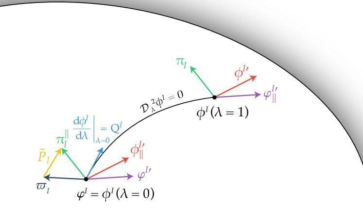
Figure 3: Schematic representation of the Hamiltonian variables on a curved field space. The full (co)vectors $\phi^{I\prime}$ and $\pi_{I}$ are defined at $\phi^{I}$, while their IR parts $\varphi^{I\prime}$ and $\varpi_{I}$ live at $\varphi^{I}$. These two points can be connected by the geodesic $\lambda$-line ${\cal D}_{\lambda}^{2}\phi^{I}(\lambda)=0$, characterised by the contravariant UV perturbation $Q^{I}=\mathrm{d}\phi^{I}/\mathrm{d}\lambda|_{\lambda=0}$ which is a vector at $\varphi^{I}$. Along this line, vectors living at each point can be parallel transported to each others (vectors in the same color). This procedure enables one to efficiently expand the action in terms of (co)vectors at the IR point $\varphi^{I}$.

Let us describe this approach in detail (see Fig. 3 for a schematic representation). We first recall that the full field $\phi^{I}$ (at $\lambda=1$) and its IR part $\varphi^{I}$ (at $\lambda=0$) are connected by a unique geodesic line

$${\cal D}_{\lambda}^{2}\phi^{I}=0,\quad\Leftrightarrow\quad\frac{\mathrm{d}^{2}\phi^{I}}{\mathrm{d}\lambda^{2}}=-\Gamma^{I}_{JK}\frac{\mathrm{d}\phi^{J}}{\mathrm{d}\lambda}\frac{\mathrm{d}\phi^{K}}{\mathrm{d}\lambda},$$ (178)

with the affine parameter $\lambda$. This geodesic line can be characterised by the contravariant vector at $\lambda=0$

$$Q^{I}:=\left.\frac{\mathrm{d}\phi^{I}}{\mathrm{d}\lambda}\right|_{\lambda=0}.$$ (179)

Then one can parallel transport, e.g., the full momentum $\pi_{I}$, a covector at $\lambda=1$, to the IR point $\lambda=0$ along this $\lambda$-line. The transport condition is given by ${\cal D}_{\lambda}\pi^{\parallel}_{I}=0$ with the initial condition $\pi^{\parallel}_{I}|_{\lambda=1}=\pi_{I}$. The transported momentum $\pi^{\parallel}_{I}|_{\lambda=0}$ is a covector at $\lambda=0$, so that it can be directly compared to the other covector there, $\varpi_{I}$. Thus one can define the covariant UV momentum by their difference, i.e.:

$${\tilde{P}}_{I}\equiv\pi^{\parallel}_{I}|_{\lambda=0}-\varpi_{I}.$$ (180)

This new definition coincides with the previous one ${\tilde{P}}_{I}={\cal D}_{\lambda}\pi_{I}|_{\lambda=0}$.

As the scalar product (computed with the field-space metric) between two parallel-transported quantities is constant, the kinetic term in the Hamiltonian, for example, can be easily expressed as

$$\pi_{I}\pi^{I}|_{\lambda=1}=\pi_{I}^{\parallel}\pi^{I}_{\parallel}|_{\lambda=0}=(\varpi_{I}+{\tilde{P}}_{I})(\varpi^{I}+{\tilde{P}}^{I}).$$ (181)

Similarly, all scalar products in the Hamiltonian action such as $\pi_{I}\pi^{I}$, $\pi_{I}{\phi^{\prime}}^{I}$, $\pi_{I}\partial_{i}\phi^{I}$, and $G_{IJ}\partial_{i}\phi^{I}\partial_{i}\phi^{J}$ can be expanded at $\lambda=0$ as $\pi_{I}^{\parallel}\pi^{I}_{\parallel}|_{\lambda=0}$, $\pi_{I}^{\parallel}{\phi^{\prime}}^{I}_{\parallel}|_{\lambda=0}$, and so on. Using the geodesic equation (178) as well as expansions around $\lambda=0$ of the Christoffel symbols and their derivatives, it is then straightforward, although tedious, to find the following expressions:

$${\phi^{\prime}}^{I}_{\parallel}|_{\lambda=0}= \,{\varphi^{\prime}}^{I}+{\cal D}_{N}Q^{I}+\frac{1}{2}R^{I}{}_{JKL}{\varphi^{\prime}}^{L}Q^{J}Q^{K}$$

$$+\frac{1}{6}R^{I}{}_{JKM;L}{\varphi^{\prime}}^{M}Q^{J}Q^{K}Q^{L}+\frac{1}{6}R^{I}{}_{JKL}Q^{J}Q^{K}{\cal D}_{N}Q^{L}+\cdots,$$ (182)

$$(\partial_{i}\phi^{I})_{\parallel}|_{\lambda=0}= \partial_{i}Q^{I}+\frac{1}{6}R^{I}{}_{JKL}Q^{J}Q^{K}\partial_{i}Q^{L}+\cdots\,.$$ (183)

The scalar potential $V$ can be also expanded in a covariant way as

$$V|_{\lambda=1} =V+V_{I}Q^{I}+\frac{1}{2}V_{;IJ}Q^{I}Q^{J}+\frac{1}{6}V_{;IJK}Q^{I}Q^{J}Q^{K}+\cdots.$$ (184)

The ADM variables $\mathcal{N}$ and $\beta^{i}$ are also scalars in field space but they should be considered independent of $\phi^{I}$ and $\pi_{I}$ before one takes into account their constraint equations. Thus, one can define their UV parts by the simple differences

$$\mathcal{N}_{\text{UV}}\equiv\mathcal{N}-\mathcal{N}_{\text{IR}},\qquad a^{-2}\partial_{i}\psi\equiv\beta^{i}-0.$$ (185)

Up to cubic order in the covariant UV perturbations $Q^{I}$ and ${\tilde{P}}_{I}$, the Hamiltonian action then reads

$$S^{(0)} =\int\mathrm{d}^{4}x\,a^{3}\left[\varpi_{I}{\varphi^{\prime}}^{I}-\frac{1}{H}\left(\frac{1}{2}\varpi_{I}\varpi^{I}+V+3M_{\text{Pl}}^{2}H^{2}\right)\right],$$ (186)

$$S^{(1)} =\int\mathrm{d}^{4}x\,a^{3}\left[{\tilde{P}}_{I,\kappa}\left({\varphi^{\prime}}^{I}-\frac{\varpi^{I}}{H}\right)-Q^{I}\left({\cal D}_{N}\varpi_{I}+3\varpi_{I}+\frac{V_{I}}{H}\right)-\mathcal{N}_{\text{UV}}\left(\frac{1}{2}\varpi_{I}\varpi^{I}+V-3M_{\text{Pl}}^{2}H^{2}\right)\right],$$ (187)

$$S^{(2)} =\int\mathrm{d}^{4}x\,a^{3}\left[{\tilde{P}}_{I,\kappa}{\cal D}_{N}Q^{I}-3M_{\text{Pl}}^{2}H^{3}\mathcal{N}_{\text{UV}}^{2}-\mathcal{N}_{\text{UV}}\left(\varpi_{I}{\tilde{P}}^{I}_{\kappa}+V_{I}Q^{I}+2M_{\text{Pl}}^{2}H^{2}\frac{\nabla^{2}}{a^{2}}\psi\right)+\varpi_{I}Q^{I}\frac{\nabla^{2}}{a^{2}}\psi\right.$$

$$\qquad-\frac{1}{H}\left(\frac{1}{2}{\tilde{P}}_{I,\kappa}{\tilde{P}}^{I}_{\kappa}-\frac{1}{2}Q_{I}\frac{\nabla^{2}}{a^{2}}Q^{I}+\frac{1}{2}V_{;IJ}Q^{I}Q^{J}-\frac{1}{2}R_{I}{}^{KL}{}_{J}\varpi_{K}\varpi_{L}Q^{I}Q^{J}\right)$$

$$\qquad\left.+\left(\frac{1}{2}-\kappa\right)\left({\varphi^{\prime}}^{I}-\frac{\varpi^{I}}{H}\right)R_{IJK}{}^{L}\varpi_{L}Q^{J}Q^{K}\right],$$ (188)

$$S^{(3)} =\int\mathrm{d}^{4}x\,a^{3}\left[3M_{\text{Pl}}^{2}H^{4}\mathcal{N}_{\text{UV}}^{3}+2M_{\text{Pl}}^{2}H^{3}\mathcal{N}_{\text{UV}}^{2}\frac{\nabla^{2}}{a^{2}}\psi+\frac{1}{2}M_{\text{Pl}}^{2}H^{2}\mathcal{N}_{\text{UV}}\left(\left(\frac{\psi_{ii}}{a^{2}}\right)^{2}-\frac{\psi_{ij}}{a^{2}}\frac{\psi_{ij}}{a^{2}}\right)\right.$$

$$\qquad-\frac{1}{a^{2}}\psi_{i}{\tilde{P}}_{I,\kappa}\partial_{i}Q^{I}-\mathcal{N}_{\text{UV}}\left(\frac{1}{2}{\tilde{P}}_{I,\kappa}{\tilde{P}}^{I}_{\kappa}+\frac{1}{2a^{2}}\partial_{i}Q^{I}\partial_{i}Q_{I}+\frac{1}{2}V_{;IJ}Q^{I}Q^{J}-\kappa R_{I}{}^{KL}{}_{J}\varpi_{K}\varpi_{L}Q^{I}Q^{J}\right)$$

$$\qquad+\mathcal{N}_{\text{IR}}\left(\left(\frac{1}{2}+\kappa\right)R^{L}{}_{IJ}{}^{K}\varpi_{L}Q^{I}Q^{J}{\tilde{P}}_{K,\kappa}-\frac{1}{6}V_{;IJK}Q^{I}Q^{J}Q^{K}+\frac{1}{6}R^{L}{}_{IJ}{}^{M}{}_{;K}\varpi_{L}\varpi_{M}Q^{I}Q^{J}Q^{K}\right)$$

$$\qquad+\frac{1}{6}\left({\varphi^{\prime}}^{I}-\frac{\varpi^{I}}{H}\right)\left(3R_{IJK}{}^{L}Q^{J}Q^{K}{\tilde{P}}_{L,\kappa}+R_{IJK}{}^{M}{}_{;L}\varpi_{M}Q^{J}Q^{K}Q^{L}\right)$$

$$\qquad\left.+\left(\frac{1}{6}-\kappa\right)R^{L}{}_{IJK}\varpi_{L}Q^{I}Q^{J}{\cal D}_{N}Q^{K}\right].$$ (189)

Here we use the generalised momentum ${\tilde{P}}_{I,\kappa}$ (175), allowing a shift from the original momentum (180). As mentioned before, $\kappa=1/2$ eliminates the term proportional to the “background-like” EoM ${\varphi^{\prime}}^{I}-\varpi^{I}/H$ in the quadratic action $S^{(2)}$. On the other hand, if one chooses $\kappa=1/6$, there is no term containing ${\cal D}_{N}Q^{I}$ in the cubic action, which indicates that ${\tilde{P}}_{I,1/6}$ might enjoy interesting properties. Although not directly used in this paper, we hope these results can be useful for future works.

Appendix C Covariant notations

We gather in this appendix the various covariant notations that we use in the paper.

C.1 Manifolds, indices and related metrics

To use compact and covariant notations, we had to introduce several types of indices denoting coordinates on various manifolds. To help the reader, here we show a comprehensive list of these notations together with the corresponding metrics that must be used to raise and lower indices.

Manifold	Index	Metric	Dimension
Spacetime	$\mu$	$g_{\mu\nu}$	$4$
$3$-dimensional spatial hypersurfaces	$i$	$\gamma_{ij}=a^{2}\delta_{ij}$ in flat gauge	$3$
Field space	$I$	$G_{IJ}$ evaluated at $\phi^{I}$ or $\varphi^{I}$	$N_{\mathrm{fields}}$
Phase space	$X$ or $\tilde{X}$	$\displaystyle-i\sigma_{2XY}=\bigl{(}\begin{smallmatrix}0&-1\\ 1&0\end{smallmatrix}\bigr{)}$	$2$
Set of creation-annihilation operators	$A$	$\delta_{AB}$	$N_{\mathrm{fields}}$
Vielbeins’ frame	$\alpha$	$\delta_{\alpha\beta}$	$N_{\mathrm{fields}}$
Mass squared matrix eigenvalues	$i$	$\delta_{ij}$	$N_{\mathrm{fields}}$
Set $\{+,-\}$ of CTP branches	$a$	$\sigma_{3ab}=\mathrm{diag}(1,-1)_{ab}$	$2$
Keldysh basis $\{\mathrm{cl},\mathrm{q}\}$	$\mathfrak{a}$	$\displaystyle\sigma_{1\mathfrak{a}\mathfrak{b}}=\bigl{(}\begin{smallmatrix}0&1\\ 1&0\end{smallmatrix}\bigr{)}$	$2$

C.2 Covariant derivatives

Motivated by our will to have a manifestly covariant theory of multifield stochastic inflation, we have to use a certain number of covariant derivatives. Here we list all of them and show their actions on an IR stochastic vector in phase space $\mathcal{U}^{I}\left(\varphi^{I},\varpi_{I}\right)$ from which their actions on any IR stochastic tensor can be deduced. Note that $A^{Q{\tilde{\mathcal{U}}}JK}=A^{Q\mathcal{U}JK}+\Gamma^{K}_{LM}\mathcal{U}^{L}A^{QQJM}$.

Name	Notation	Action on a field-space vector
Field space	$\nabla_{J}$	$\nabla_{J}\mathcal{U}^{I}=\partial_{J}\mathcal{U}^{I}+\Gamma^{I}_{JK}\mathcal{U}^{K}$
Phase space	$D_{\varphi^{J}}$	$D_{\varphi^{J}}\mathcal{U}^{I}=\nabla_{J}\mathcal{U}^{I}+\Gamma^{K}_{JL}\varpi_{K}\partial_{\varpi_{L}}\mathcal{U}^{I}$
Time (deterministic or Stratonovich scheme)	${\cal D}_{N}$	${\cal D}_{N}\mathcal{U}^{I}=\partial_{N}\mathcal{U}^{I}+\Gamma^{I}_{JK}\left(\partial_{N}\varphi^{J}\right)\mathcal{U}^{K}$
Time (Itô scheme)	$\mathfrak{D}_{N}$	$\displaystyle\mathfrak{D}_{N}\mathcal{U}^{I}={\cal D}_{N}\mathcal{U}^{I}+\frac{1}{2}\left(\Gamma^{I}_{JS,K}-\Gamma^{M}_{JS}\Gamma^{I}_{MK}\right)\mathcal{U}^{S}A^{QQJK}+\Gamma^{I}_{JK}A^{Q{\tilde{\mathcal{U}}}JK}$

C.3 Covariant perturbations?

Under redefinitions of the scalar fields, naive perturbations of the full fields $\phi^{I}$ and $\pi_{I}$ around a classical background (or IR) value, do not transform covariantly beyond linear order. This subtlety was discussed in Sec. 4.2 and in Appendix B. Here we summarise our notations for “perturbations” including the naive ones, $\delta\phi^{I}=\phi^{I}-\varphi^{I}$ and $\delta\pi_{I}=\pi_{I}-\varpi_{I}$, as well as the true covariant objects such as $Q^{I}$ and ${\tilde{P}}_{I}$. Their covariance (“Yes”, “No”, or at “Linear order” only) is also explicitly shown.

Notation	Definition	Covariant?
$\delta\phi^{I}$	$\displaystyle\phi^{I}-\varphi^{I}=Q^{I}-\frac{1}{2}\Gamma^{I}_{JK}Q^{J}Q^{K}+\cdots$	Linear order
$\delta\pi_{I}$	$\begin{aligned} \pi_{I}-\varpi_{I}=&\,{\tilde{P}}_{I}+\Gamma_{IJ}^{K}\varpi_{K}Q^{J}+\Gamma^{K}_{IJ}Q^{J}{\tilde{P}}_{K}\\ &+\frac{1}{2}(\Gamma^{S}_{IJ,K}-\Gamma^{S}_{IR}\Gamma^{R}_{JK}+\Gamma^{R}_{IJ}\Gamma^{S}_{RK})\varpi_{S}Q^{J}Q^{K}+\cdots\end{aligned}$	No
$Q^{I}$	$\displaystyle\left.\frac{\mathrm{d}\phi^{I}}{\mathrm{d}\lambda}\right|_{\lambda=0}$	Yes
$P_{I}$	$\displaystyle\left.\frac{\mathrm{d}\pi_{I}}{\mathrm{d}\lambda}\right|_{\lambda=0}$	No
${\tilde{P}}_{I}$	${\cal D}_{\lambda}\pi_{I}|_{\lambda=0}=P_{I}-\Gamma^{K}_{IJ}\varpi_{K}Q^{J}$	Yes
${\tilde{P}}_{I,\kappa}$	${\tilde{P}}_{I}+\kappa R_{IJK}{}^{L}\varpi_{L}Q^{J}Q^{K}$	Yes

References

- (1) Planck collaboration, Planck 2018 results. X. Constraints on inflation, 1807.06211.
- (2) Planck collaboration, Planck 2018 results. IX. Constraints on primordial non-Gaussianity, 1905.05697.
- (3) D. Baumann and L. McAllister, Inflation and String Theory. Cambridge University Press, 2015, [1404.2601].
- (4) D. Wands, Local non-Gaussianity from inflation, Class. Quant. Grav. 27 (2010) 124002 [1004.0818].
- (5) X. Chen, Primordial Non-Gaussianities from Inflation Models, Adv. Astron. 2010 (2010) 638979 [1002.1416].
- (6) Y. Wang, Inflation, Cosmic Perturbations and Non-Gaussianities, Commun. Theor. Phys. 62 (2014) 109 [1303.1523].
- (7) S. Renaux-Petel, Primordial non-Gaussianities after Planck 2015: an introductory review, Comptes Rendus Physique 16 (2015) 969 [1508.06740].
- (8) P. D. Meerburg et al., Primordial Non-Gaussianity, 1903.04409.
- (9) D. H. Lyth and A. Riotto, Particle physics models of inflation and the cosmological density perturbation, Phys. Rept. 314 (1999) 1 [hep-ph/9807278].
- (10) S. Cremonini, Z. Lalak and K. Turzynski, Strongly Coupled Perturbations in Two-Field Inflationary Models, JCAP 1103 (2011) 016 [1010.3021].
- (11) S. Renaux-Petel and K. Turzynski, On reaching the adiabatic limit in multi-field inflation, JCAP 06 (2015) 010 [1405.6195].
- (12) J. J. M. Carrasco, R. Kallosh, A. Linde and D. Roest, Hyperbolic geometry of cosmological attractors, Phys. Rev. D 92 (2015) 041301 [1504.05557].
- (13) S. Renaux-Petel and K. Turzyński, Geometrical Destabilization of Inflation, Phys. Rev. Lett. 117 (2016) 141301 [1510.01281].
- (14) A. Hetz and G. A. Palma, Sound Speed of Primordial Fluctuations in Supergravity Inflation, Phys. Rev. Lett. 117 (2016) 101301 [1601.05457].
- (15) A. Achúcarro, V. Atal, C. Germani and G. A. Palma, Cumulative effects in inflation with ultra-light entropy modes, JCAP 1702 (2017) 013 [1607.08609].
- (16) Y. Tada and V. Vennin, Squeezed bispectrum in the formalism: local observer effect in field space, JCAP 02 (2017) 021 [1609.08876].
- (17) A. R. Brown, Hyperbolic Inflation, Phys. Rev. Lett. 121 (2018) 251601 [1705.03023].
- (18) S. Renaux-Petel, K. Turzyński and V. Vennin, Geometrical destabilization, premature end of inflation and Bayesian model selection, JCAP 1711 (2017) 006 [1706.01835].
- (19) S. Mizuno and S. Mukohyama, Primordial perturbations from inflation with a hyperbolic field-space, Phys. Rev. D96 (2017) 103533 [1707.05125].
- (20) A. Achúcarro, R. Kallosh, A. Linde, D.-G. Wang and Y. Welling, Universality of multi-field -attractors, JCAP 1804 (2018) 028 [1711.09478].
- (21) T. Krajewski, K. Turzyński and M. Wieczorek, On preheating in -attractor models of inflation, 1801.01786.
- (22) P. Christodoulidis, D. Roest and E. I. Sfakianakis, Angular inflation in multi-field -attractors, 1803.09841.
- (23) A. Linde, D.-G. Wang, Y. Welling, Y. Yamada and A. Achúcarro, Hypernatural inflation, JCAP 1807 (2018) 035 [1803.09911].
- (24) S. Garcia-Saenz, S. Renaux-Petel and J. Ronayne, Primordial fluctuations and non-Gaussianities in sidetracked inflation, JCAP 1807 (2018) 057 [1804.11279].
- (25) S. Garcia-Saenz and S. Renaux-Petel, Flattened non-Gaussianities from the effective field theory of inflation with imaginary speed of sound, JCAP 1811 (2018) 005 [1805.12563].
- (26) A. Achúcarro and G. A. Palma, The string swampland constraints require multi-field inflation, JCAP 1902 (2019) 041 [1807.04390].
- (27) A. Achúcarro, S. Céspedes, A.-C. Davis and G. A. Palma, Constraints on Holographic Multifield Inflation and Models Based on the Hamilton-Jacobi Formalism, Phys. Rev. Lett. 122 (2019) 191301 [1809.05341].
- (28) A. Achúcarro, E. J. Copeland, O. Iarygina, G. A. Palma, D.-G. Wang and Y. Welling, Shift-Symmetric Orbital Inflation: single field or multi-field?, 1901.03657.
- (29) T. Bjorkmo and M. C. D. Marsh, Hyperinflation generalised: from its attractor mechanism to its tension with the ‘swampland conditions’, JHEP 04 (2019) 172 [1901.08603].
- (30) O. Grocholski, M. Kalinowski, M. Kolanowski, S. Renaux-Petel, K. Turzyński and V. Vennin, On backreaction effects in geometrical destabilisation of inflation, JCAP 1905 (2019) 008 [1901.10468].
- (31) J. Fumagalli, S. Garcia-Saenz, L. Pinol, S. Renaux-Petel and J. Ronayne, Hyper non-Gaussianities in inflation with strongly non-geodesic motion, 1902.03221.
- (32) T. Bjorkmo, The rapid-turn inflationary attractor, Phys. Rev. Lett. 122 (2019) 251301 [1902.10529].
- (33) P. Christodoulidis, D. Roest and E. I. Sfakianakis, Attractors, Bifurcations and Curvature in Multi-field Inflation, JCAP 08 (2020) 006 [1903.03513].
- (34) P. Christodoulidis, D. Roest and E. I. Sfakianakis, Scaling attractors in multi-field inflation, 1903.06116.
- (35) V. Aragam, S. Paban and R. Rosati, Multi-field Inflation in High-Slope Potentials, 1905.07495.
- (36) S. Mizuno, S. Mukohyama, S. Pi and Y.-L. Zhang, Hyperbolic field space and swampland conjecture for DBI scalar, 1905.10950.
- (37) R. Bravo, G. A. Palma and S. Riquelme, A Tip for Landscape Riders: Multi-Field Inflation Can Fulfill the Swampland Distance Conjecture, 1906.05772.
- (38) A. Achúcarro and Y. Welling, Orbital Inflation: inflating along an angular isometry of field space, 1907.02020.
- (39) S. Garcia-Saenz, L. Pinol and S. Renaux-Petel, Revisiting non-Gaussianity in multifield inflation with curved field space, 1907.10403.
- (40) D. Chakraborty, R. Chiovoloni, O. Loaiza-Brito, G. Niz and I. Zavala, Fat inflatons, large turns and the -problem, JCAP 01 (2020) 020 [1908.09797].
- (41) T. Bjorkmo, R. Z. Ferreira and M. D. Marsh, Mild Non-Gaussianities under Perturbative Control from Rapid-Turn Inflation Models, JCAP 12 (2019) 036 [1908.11316].
- (42) D.-G. Wang, On the inflationary massive field with a curved field manifold, JCAP 01 (2020) 046 [1911.04459].
- (43) R. Z. Ferreira, Non-Gaussianities in models of inflation with large and negative entropic masses, 2003.13410.
- (44) M. Braglia, D. K. Hazra, L. Sriramkumar and F. Finelli, Generating primordial features at large scales in two field models of inflation, 2004.00672.
- (45) G. A. Palma, S. Sypsas and C. Zenteno, Seeding primordial black holes in multi-field inflation, 2004.06106.
- (46) J. Fumagalli, S. Renaux-Petel, J. W. Ronayne and L. T. Witkowski, Turning in the landscape: a new mechanism for generating Primordial Black Holes, 2004.08369.
- (47) M. Braglia, D. K. Hazra, F. Finelli, G. F. Smoot, L. Sriramkumar and A. A. Starobinsky, Generating PBHs and small-scale GWs in two-field models of inflation, 2005.02895.
- (48) A. Starobinsky, Dynamics of phase transition in the new inflationary universe scenario and generation of perturbations, Physics Letters B 117 (1982) 175 .
- (49) A. A. Starobinsky, STOCHASTIC DE SITTER (INFLATIONARY) STAGE IN THE EARLY UNIVERSE, Lect. Notes Phys. 246 (1986) 107.
- (50) Y. Nambu and M. Sasaki, Stochastic stage of an inflationary universe model, Physics Letters B 205 (1988) 441 .
- (51) Y. Nambu and M. Sasaki, Stochastic approach to chaotic inflation and the distribution of universes, Physics Letters B 219 (1989) 240 .
- (52) H. E. Kandrup, STOCHASTIC INFLATION AS A TIME DEPENDENT RANDOM WALK, Phys. Rev. D 39 (1989) 2245.
- (53) K.-i. Nakao, Y. Nambu and M. Sasaki, Stochastic Dynamics of New Inflation, Prog. Theor. Phys. 80 (1988) 1041.
- (54) Y. Nambu, Stochastic Dynamics of an Inflationary Model and Initial Distribution of Universes, Prog. Theor. Phys. 81 (1989) 1037.
- (55) S. Mollerach, S. Matarrese, A. Ortolan and F. Lucchin, Stochastic inflation in a simple two field model, Phys. Rev. D 44 (1991) 1670.
- (56) A. D. Linde, D. A. Linde and A. Mezhlumian, From the Big Bang theory to the theory of a stationary universe, Phys. Rev. D 49 (1994) 1783 [gr-qc/9306035].
- (57) A. A. Starobinsky and J. Yokoyama, Equilibrium state of a selfinteracting scalar field in the De Sitter background, Phys. Rev. D50 (1994) 6357 [astro-ph/9407016].
- (58) N. Tsamis and R. Woodard, Stochastic quantum gravitational inflation, Nucl. Phys. B 724 (2005) 295 [gr-qc/0505115].
- (59) T. Prokopec, N. Tsamis and R. Woodard, Stochastic Inflationary Scalar Electrodynamics, Annals Phys. 323 (2008) 1324 [0707.0847].
- (60) F. Finelli, G. Marozzi, A. Starobinsky, G. Vacca and G. Venturi, Generation of fluctuations during inflation: Comparison of stochastic and field-theoretic approaches, Phys. Rev. D 79 (2009) 044007 [0808.1786].
- (61) F. Finelli, G. Marozzi, A. Starobinsky, G. Vacca and G. Venturi, Stochastic growth of quantum fluctuations during slow-roll inflation, Phys. Rev. D 82 (2010) 064020 [1003.1327].
- (62) B. Garbrecht, G. Rigopoulos and Y. Zhu, Infrared correlations in de Sitter space: Field theoretic versus stochastic approach, Phys. Rev. D 89 (2014) 063506 [1310.0367].
- (63) B. Garbrecht, F. Gautier, G. Rigopoulos and Y. Zhu, Feynman Diagrams for Stochastic Inflation and Quantum Field Theory in de Sitter Space, Phys. Rev. D 91 (2015) 063520 [1412.4893].
- (64) V. Onemli, Vacuum Fluctuations of a Scalar Field during Inflation: Quantum versus Stochastic Analysis, Phys. Rev. D 91 (2015) 103537 [1501.05852].
- (65) G. Cho, C. H. Kim and H. Kitamoto, Stochastic Dynamics of Infrared Fluctuations in Accelerating Universe, in 2nd LeCosPA Symposium: Everything about Gravity, Celebrating the Centenary of Einstein’s General Relativity, pp. 162–167, 2017, 1508.07877, DOI.
- (66) D. Seery, One-loop corrections to a scalar field during inflation, JCAP 11 (2007) 025 [0707.3377].
- (67) K. Enqvist, S. Nurmi, D. Podolsky and G. Rigopoulos, On the divergences of inflationary superhorizon perturbations, JCAP 04 (2008) 025 [0802.0395].
- (68) D. Seery, A parton picture of de Sitter space during slow-roll inflation, J. Cosmology Astropart. Phys 2009 (2009) 021 [0903.2788].
- (69) C. Burgess, L. Leblond, R. Holman and S. Shandera, Super-Hubble de Sitter Fluctuations and the Dynamical RG, JCAP 03 (2010) 033 [0912.1608].
- (70) D. Seery, Infrared effects in inflationary correlation functions, Class. Quant. Grav. 27 (2010) 124005 [1005.1649].
- (71) F. Gautier and J. Serreau, Infrared dynamics in de Sitter space from Schwinger-Dyson equations, Phys. Lett. B 727 (2013) 541 [1305.5705].
- (72) M. Guilleux and J. Serreau, Quantum scalar fields in de Sitter space from the nonperturbative renormalization group, Phys. Rev. D 92 (2015) 084010 [1506.06183].
- (73) F. Gautier and J. Serreau, Scalar field correlator in de Sitter space at next-to-leading order in a 1/N expansion, Phys. Rev. D 92 (2015) 105035 [1509.05546].
- (74) T. Markkanen, Renormalization of the inflationary perturbations revisited, JCAP 05 (2018) 001 [1712.02372].
- (75) D. López Nacir, F. D. Mazzitelli and L. G. Trombetta, To the sphere and back again: de Sitter infrared correlators at NTLO in 1/N, JHEP 08 (2019) 052 [1905.03665].
- (76) V. Gorbenko and L. Senatore, in dS, 1911.00022.
- (77) M. Mirbabayi, Infrared dynamics of a light scalar field in de Sitter, 1911.00564.
- (78) P. Adshead, L. Pearce, J. Shelton and Z. J. Weiner, Stochastic evolution of scalar fields with continuous symmetries during inflation, Phys. Rev. D 102 (2020) 023526 [2002.07201].
- (79) G. Moreau, J. Serreau and C. Noûs, The expansion for stochastic fields in de Sitter spacetime, 2004.09157.
- (80) T. Cohen and D. Green, Soft de Sitter Effective Theory, 2007.03693.
- (81) A. D. Linde, ETERNAL CHAOTIC INFLATION, Mod. Phys. Lett. A1 (1986) 81.
- (82) A. D. Linde, Eternally Existing Selfreproducing Chaotic Inflationary Universe, Phys. Lett. B175 (1986) 395.
- (83) A. S. Goncharov, A. D. Linde and V. F. Mukhanov, The Global Structure of the Inflationary Universe, Int. J. Mod. Phys. A2 (1987) 561.
- (84) D. Wands, K. A. Malik, D. H. Lyth and A. R. Liddle, A new approach to the evolution of cosmological perturbations on large scales, Phys. Rev. D62 (2000) 043527 [astro-ph/0003278].
- (85) D. S. Salopek and J. R. Bond, Nonlinear evolution of long wavelength metric fluctuations in inflationary models, Phys. Rev. D42 (1990) 3936.
- (86) M. Sasaki and E. D. Stewart, A General analytic formula for the spectral index of the density perturbations produced during inflation, Prog. Theor. Phys. 95 (1996) 71 [astro-ph/9507001].
- (87) M. Sasaki and T. Tanaka, Super-horizon scale dynamics of multi-scalar inflation, Prog. Theor. Phys. 99 (1998) 763 [gr-qc/9801017].
- (88) D. H. Lyth, K. A. Malik and M. Sasaki, A General proof of the conservation of the curvature perturbation, JCAP 0505 (2005) 004 [astro-ph/0411220].
- (89) T. Fujita, M. Kawasaki, Y. Tada and T. Takesako, A new algorithm for calculating the curvature perturbations in stochastic inflation, JCAP 1312 (2013) 036 [1308.4754].
- (90) T. Fujita, M. Kawasaki and Y. Tada, Non-perturbative approach for curvature perturbations in stochastic formalism, JCAP 1410 (2014) 030 [1405.2187].
- (91) V. Vennin and A. A. Starobinsky, Correlation Functions in Stochastic Inflation, Eur. Phys. J. C75 (2015) 413 [1506.04732].
- (92) M. Kawasaki and Y. Tada, Can massive primordial black holes be produced in mild waterfall hybrid inflation?, JCAP 08 (2016) 041 [1512.03515].
- (93) H. Assadullahi, H. Firouzjahi, M. Noorbala, V. Vennin and D. Wands, Multiple Fields in Stochastic Inflation, JCAP 06 (2016) 043 [1604.04502].
- (94) V. Vennin, H. Assadullahi, H. Firouzjahi, M. Noorbala and D. Wands, Critical Number of Fields in Stochastic Inflation, Phys. Rev. Lett. 118 (2017) 031301 [1604.06017].
- (95) L. Pinol, S. Renaux-Petel and Y. Tada, Inflationary stochastic anomalies, Class. Quant. Grav. 36 (2019) 07LT01 [1806.10126].
- (96) G. Rigopoulos and E. Shellard, The separate universe approach and the evolution of nonlinear superhorizon cosmological perturbations, Phys. Rev. D 68 (2003) 123518 [astro-ph/0306620].
- (97) G. I. Rigopoulos and E. Shellard, Non-linear inflationary perturbations, JCAP 10 (2005) 006 [astro-ph/0405185].
- (98) G. Rigopoulos, E. Shellard and B. van Tent, A Simple route to non-Gaussianity in inflation, Phys. Rev. D 72 (2005) 083507 [astro-ph/0410486].
- (99) G. Rigopoulos, E. Shellard and B. van Tent, Non-linear perturbations in multiple-field inflation, Phys. Rev. D 73 (2006) 083521 [astro-ph/0504508].
- (100) G. Rigopoulos, E. Shellard and B. van Tent, Large non-Gaussianity in multiple-field inflation, Phys. Rev. D 73 (2006) 083522 [astro-ph/0506704].
- (101) C. Pattison, V. Vennin, H. Assadullahi and D. Wands, Quantum diffusion during inflation and primordial black holes, JCAP 10 (2017) 046 [1707.00537].
- (102) J. M. Ezquiaga and J. García-Bellido, Quantum diffusion beyond slow-roll: implications for primordial black-hole production, 1805.06731.
- (103) M. Biagetti, G. Franciolini, A. Kehagias and A. Riotto, Primordial Black Holes from Inflation and Quantum Diffusion, JCAP 07 (2018) 032 [1804.07124].
- (104) J. M. Ezquiaga, J. García-Bellido and V. Vennin, The exponential tail of inflationary fluctuations: consequences for primordial black holes, JCAP 03 (2020) 029 [1912.05399].
- (105) G. Panagopoulos and E. Silverstein, Primordial Black Holes from non-Gaussian tails, 1906.02827.
- (106) J. S. Bullock and J. R. Primack, NonGaussian fluctuations and primordial black holes from inflation, Phys. Rev. D 55 (1997) 7423 [astro-ph/9611106].
- (107) J. Garcia-Bellido, A. D. Linde and D. Wands, Density perturbations and black hole formation in hybrid inflation, Phys. Rev. D 54 (1996) 6040 [astro-ph/9605094].
- (108) P. Ivanov, Nonlinear metric perturbations and production of primordial black holes, Phys. Rev. D 57 (1998) 7145 [astro-ph/9708224].
- (109) J. Yokoyama, Chaotic new inflation and formation of primordial black holes, Phys. Rev. D 58 (1998) 083510 [astro-ph/9802357].
- (110) S. Bird, I. Cholis, J. B. Muñoz, Y. Ali-Haïmoud, M. Kamionkowski, E. D. Kovetz et al., Did LIGO detect dark matter?, Phys. Rev. Lett. 116 (2016) 201301 [1603.00464].
- (111) S. Clesse and J. García-Bellido, The clustering of massive Primordial Black Holes as Dark Matter: measuring their mass distribution with Advanced LIGO, Phys. Dark Univ. 15 (2017) 142 [1603.05234].
- (112) M. Sasaki, T. Suyama, T. Tanaka and S. Yokoyama, Primordial Black Hole Scenario for the Gravitational-Wave Event GW150914, Phys. Rev. Lett. 117 (2016) 061101 [1603.08338].
- (113) B. Carr, F. Kuhnel and M. Sandstad, Primordial Black Holes as Dark Matter, Phys. Rev. D 94 (2016) 083504 [1607.06077].
- (114) B. Carr, K. Kohri, Y. Sendouda and J. Yokoyama, Constraints on Primordial Black Holes, 2002.12778.
- (115) H. Niikura, M. Takada, S. Yokoyama, T. Sumi and S. Masaki, Constraints on Earth-mass primordial black holes from OGLE 5-year microlensing events, Phys. Rev. D 99 (2019) 083503 [1901.07120].
- (116) J. Scholtz and J. Unwin, What if Planet 9 is a Primordial Black Hole?, 1909.11090.
- (117) E. Witten, Searching for a Black Hole in the Outer Solar System, 2004.14192.
- (118) J. Garcia-Bellido, A. D. Linde and D. A. Linde, Fluctuations of the gravitational constant in the inflationary Brans-Dicke cosmology, Phys. Rev. D 50 (1994) 730 [astro-ph/9312039].
- (119) J. Garcia-Bellido, Jordan-Brans-Dicke stochastic inflation, Nucl. Phys. B 423 (1994) 221 [astro-ph/9401042].
- (120) J. Garcia-Bellido and A. D. Linde, Stationary solutions in Brans-Dicke stochastic inflationary cosmology, Phys. Rev. D 52 (1995) 6730 [gr-qc/9504022].
- (121) R. P. Feynman and F. L. Vernon, Jr., The Theory of a general quantum system interacting with a linear dissipative system, Annals Phys. 24 (1963) 118.
- (122) M. Morikawa, Dissipation and Fluctuation of Quantum Fields in Expanding Universes, Phys. Rev. D42 (1990) 1027.
- (123) E. A. Calzetta, B. L. Hu and F. D. Mazzitelli, Coarse grained effective action and renormalization group theory in semiclassical gravity and cosmology, Phys. Rept. 352 (2001) 459 [hep-th/0102199].
- (124) S. Matarrese, M. A. Musso and A. Riotto, Influence of superhorizon scales on cosmological observables generated during inflation, JCAP 0405 (2004) 008 [hep-th/0311059].
- (125) M. Liguori, S. Matarrese, M. Musso and A. Riotto, Stochastic inflation and the lower multipoles in the CMB anisotropies, JCAP 0408 (2004) 011 [astro-ph/0405544].
- (126) L. Perreault Levasseur, Lagrangian formulation of stochastic inflation: Langevin equations, one-loop corrections and a proposed recursive approach, Phys. Rev. D88 (2013) 083537 [1304.6408].
- (127) L. Perreault Levasseur, V. Vennin and R. Brandenberger, Recursive Stochastic Effects in Valley Hybrid Inflation, Phys. Rev. D 88 (2013) 083538 [1307.2575].
- (128) L. Perreault Levasseur and E. McDonough, Backreaction and Stochastic Effects in Single Field Inflation, Phys. Rev. D 91 (2015) 063513 [1409.7399].
- (129) I. Moss and G. Rigopoulos, Effective long wavelength scalar dynamics in de Sitter, JCAP 1705 (2017) 009 [1611.07589].
- (130) J. Tokuda and T. Tanaka, Statistical nature of infrared dynamics on de Sitter background, 1708.01734.
- (131) T. Prokopec and G. Rigopoulos, Functional renormalization group for stochastic inflation, JCAP 08 (2018) 013 [1710.07333].
- (132) J. Tokuda and T. Tanaka, Can all the infrared secular growth really be understood as increase of classical statistical variance?, JCAP 1811 (2018) 022 [1806.03262].
- (133) E. Calzetta and B. Hu, Quantum fluctuations, decoherence of the mean field, and structure formation in the early universe, Phys. Rev. D 52 (1995) 6770 [gr-qc/9505046].
- (134) E. Calzetta and B.-L. Hu, Stochastic behavior of effective field theories across threshold, Phys. Rev. D 55 (1997) 3536 [hep-th/9603164].
- (135) E. Calzetta and B. Hu, Stochastic dynamics of correlations in quantum field theory: From Schwinger-Dyson to Boltzmann-Langevin equation, Phys. Rev. D 61 (2000) 025012 [hep-ph/9903291].
- (136) M. Parikh, F. Wilczek and G. Zahariade, The Noise of Gravitons, 2005.07211.
- (137) S. Weinberg, The Quantum theory of fields. Vol. 1: Foundations, .
- (138) J. S. Schwinger, Brownian motion of a quantum oscillator, J. Math. Phys. 2 (1961) 407.
- (139) L. V. Keldysh, Diagram technique for nonequilibrium processes, Zh. Eksp. Teor. Fiz. 47 (1964) 1515.
- (140) A. Kamenev, Field theory of non-equilibrium systems. Cambridge University Press, Jan., 2011, 10.1017/CBO9781139003667.
- (141) E. A. Calzetta and B.-L. B. Hu, Nonequilibrium Quantum Field Theory, Cambridge Monographs on Mathematical Physics. Cambridge University Press, 9, 2008, 10.1017/CBO9780511535123.
- (142) A. Altland and B. D. Simons, Condensed Matter Field Theory. Cambridge University Press, 2 ed., 2010, 10.1017/CBO9780511789984.
- (143) C. Burgess, R. Holman, G. Tasinato and M. Williams, EFT Beyond the Horizon: Stochastic Inflation and How Primordial Quantum Fluctuations Go Classical, JHEP 03 (2015) 090 [1408.5002].
- (144) C. Burgess, R. Holman and G. Tasinato, Open EFTs, IR effects & late-time resummations: systematic corrections in stochastic inflation, JHEP 01 (2016) 153 [1512.00169].
- (145) H. Collins, R. Holman and T. Vardanyan, The quantum Fokker-Planck equation of stochastic inflation, JHEP 11 (2017) 065 [1706.07805].
- (146) T. Hollowood and J. McDonald, Decoherence, discord and the quantum master equation for cosmological perturbations, Phys. Rev. D 95 (2017) 103521 [1701.02235].
- (147) K. Itô, 109. stochastic integral, Proceedings of the Imperial Academy 20 (1944) 519.
- (148) R. Stratonovich, A new representation for stochastic integrals and equations, SIAM Journal on Control 4 (1966) 362.
- (149) A. Mezhlumian and A. A. Starobinsky, Stochastic inflation: New results, in The First International A.D. Sakharov Conference on Physics, 10, 1991, astro-ph/9406045.
- (150) A. Vilenkin, On the factor ordering problem in stochastic inflation, Phys. Rev. D 59 (1999) 123506 [gr-qc/9902007].
- (151) D. Ryter and U. Deker, Properties of the noise-induced “spurious”drift. i., Journal of Mathematical Physics 21 (1980) 2662.
- (152) U. Deker and D. Ryter, Properties of the noise-induced “spurious”drift. ii. simplifications of langevin equations, Journal of Mathematical Physics 21 (1980) 2666.
- (153) N. G. van Kampen, Itô versus stratonovich, Journal of Statistical Physics 24 (1981) 175.
- (154) N. van Kampen, Brownian motion on a manifold, J Stat Phys 44: 1 (1986) .
- (155) R. Graham, Covariant stochastic calculus in the sense of itô, Physics Letters A 109 (1985) 209 .
- (156) H. Kitamoto, Infrared resummation for derivative interactions in de Sitter space, Phys. Rev. D 100 (2019) 025020 [1811.01830].
- (157) S. Habib, Stochastic inflation: The Quantum phase space approach, Phys. Rev. D46 (1992) 2408 [gr-qc/9208006].
- (158) A. J. Tolley and M. Wyman, Stochastic Inflation Revisited: Non-Slow Roll Statistics and DBI Inflation, JCAP 0804 (2008) 028 [0801.1854].
- (159) K. Enqvist, D. G. Figueroa and G. Rigopoulos, Fluctuations along supersymmetric flat directions during Inflation, JCAP 01 (2012) 053 [1109.3024].
- (160) M. Kawasaki and T. Takesako, Stochastic Approach to Flat Direction during Inflation, JCAP 08 (2012) 031 [1207.1165].
- (161) G. Rigopoulos, Thermal Interpretation of Infrared Dynamics in de Sitter, JCAP 07 (2016) 035 [1604.04313].
- (162) J. Grain and V. Vennin, Stochastic inflation in phase space: Is slow roll a stochastic attractor?, JCAP 1705 (2017) 045 [1703.00447].
- (163) D. Cruces, C. Germani and T. Prokopec, Failure of the stochastic approach to inflation beyond slow-roll, JCAP 03 (2019) 048 [1807.09057].
- (164) H. Firouzjahi, A. Nassiri-Rad and M. Noorbala, Stochastic Ultra Slow Roll Inflation, JCAP 01 (2019) 040 [1811.02175].
- (165) C. Pattison, V. Vennin, H. Assadullahi and D. Wands, Stochastic inflation beyond slow roll, JCAP 1907 (2019) 031 [1905.06300].
- (166) J. Fumagalli, S. Renaux-Petel and J. W. Ronayne, Higgs vacuum (in)stability during inflation: the dangerous relevance of de Sitter departure and Planck-suppressed operators, JHEP 02 (2020) 142 [1910.13430].
- (167) T. Prokopec and G. Rigopoulos, and the stochastic conveyor belt of Ultra Slow-Roll, 1910.08487.
- (168) G. Ballesteros, J. Rey, M. Taoso and A. Urbano, Stochastic inflationary dynamics beyond slow-roll and consequences for primordial black hole formation, 2006.14597.
- (169) R. L. Arnowitt, S. Deser and C. W. Misner, The Dynamics of general relativity, Gen. Rel. Grav. 40 (2008) 1997 [gr-qc/0405109].
- (170) D. Langlois, Hamiltonian formalism and gauge invariance for linear perturbations in inflation, Class. Quant. Grav. 11 (1994) 389.
- (171) S. Winitzki and A. Vilenkin, Effective noise in stochastic description of inflation, Phys. Rev. D61 (2000) 084008 [gr-qc/9911029].
- (172) T. Markkanen, A. Rajantie, S. Stopyra and T. Tenkanen, Scalar correlation functions in de Sitter space from the stochastic spectral expansion, JCAP 08 (2019) 001 [1904.11917].
- (173) T. Markkanen and A. Rajantie, Scalar correlation functions for a double-well potential in de Sitter space, JCAP 03 (2020) 049 [2001.04494].
- (174) G. Moreau and J. Serreau, Unequal Time Correlators of Stochastic Scalar Fields in de Sitter Space, Phys. Rev. D 101 (2020) 045015 [1912.05358].
- (175) D. Boyanovsky, H. de Vega, R. Holman, D. Lee and A. Singh, Dissipation via particle production in scalar field theories, Phys. Rev. D 51 (1995) 4419 [hep-ph/9408214].
- (176) J. Rau and B. Muller, From reversible quantum microdynamics to irreversible quantum transport, Phys. Rept. 272 (1996) 1 [nucl-th/9505009].
- (177) D. Boyanovsky, H. J. de Vega, R. Holman, S. Kumar and R. D. Pisarski, Real time relaxation of condensates and kinetics in hot scalar QED: Landau damping, Phys. Rev. D 58 (1998) 125009 [hep-ph/9802370].
- (178) Z. Xu and C. Greiner, Stochastic treatment of disoriented chiral condensates within a Langevin description, Phys. Rev. D 62 (2000) 036012 [hep-ph/9910562].
- (179) A. Berera, I. G. Moss and R. O. Ramos, Local Approximations for Effective Scalar Field Equations of Motion, Phys. Rev. D 76 (2007) 083520 [0706.2793].
- (180) R. Farias, R. O. Ramos and L. da Silva, Stochastic Langevin equations: Markovian and non-Markovian dynamics, Phys. Rev. E 80 (2009) 031143 [0909.2671].
- (181) R. Farias, R. O. Ramos and L. da Silva, Numerical solutions for non-Markovian stochastic equations of motion, Comput. Phys. Commun. 180 (2009) 574 [0909.2876].
- (182) F. Gautier and J. Serreau, On the Langevin description of nonequilibrium quantum fields, Phys. Rev. D 86 (2012) 125002 [1209.1827].
- (183) G. Buldgen, M. Drewes, J. U. Kang and U. R. Mun, General Markovian Equation for Scalar Fields in a Slowly Evolving Background, 1912.02772.
- (184) H. Risken and H. Haken, The Fokker-Planck Equation: Methods of Solution and Applications Second Edition. Springer, 1989.
- (185) N. V. Kampen, Stochastic processes in physics and chemistry. North Holland, 2007.
- (186) D. S. Salopek, J. R. Bond and J. M. Bardeen, Designing Density Fluctuation Spectra in Inflation, Phys. Rev. D40 (1989) 1753.
- (187) S. Groot Nibbelink and B. van Tent, Scalar perturbations during multiple field slow-roll inflation, Class. Quant. Grav. 19 (2002) 613 [hep-ph/0107272].
- (188) S. Tsujikawa, D. Parkinson and B. A. Bassett, Correlation - consistency cartography of the double inflation landscape, Phys. Rev. D 67 (2003) 083516 [astro-ph/0210322].
- (189) S. Weinberg, Cosmology. Oxford Univ. Press, 2008.
- (190) L. P. Grishchuk and Y. V. Sidorov, Squeezed quantum states of relic gravitons and primordial density fluctuations, Phys. Rev. D 42 (1990) 3413.
- (191) A. Albrecht, P. Ferreira, M. Joyce and T. Prokopec, Inflation and squeezed quantum states, Physical Review D 50 (1994) 4807–4820.
- (192) D. Polarski and A. A. Starobinsky, Semiclassicality and decoherence of cosmological perturbations, Class. Quant. Grav. 13 (1996) 377 [gr-qc/9504030].
- (193) C. KIEFER, D. POLARSKI and A. A. STAROBINSKY, Quantum-to-classical transition for fluctuations in the early universe, International Journal of Modern Physics D 07 (1998) 455–462.
- (194) D. SUDARSKY, Shortcomings in the understanding of why cosmological perturbations look classical, International Journal of Modern Physics D 20 (2011) 509–552.
- (195) J. Martin and V. Vennin, Quantum discord of cosmic inflation: Can we show that cmb anisotropies are of quantum-mechanical origin?, Physical Review D 93 (2016) .
- (196) J. Martin, Cosmic inflation, quantum information and the pioneering role of john s bell in cosmology, 2019.
- (197) A. Ashtekar, A. Corichi and A. Kesavan, Emergence of classical behavior in the early universe, 2020.
- (198) C. Gordon, D. Wands, B. A. Bassett and R. Maartens, Adiabatic and entropy perturbations from inflation, Phys. Rev. D63 (2001) 023506 [astro-ph/0009131].
- (199) R. D. Jordan, Effective Field Equations for Expectation Values, Phys. Rev. D33 (1986) 444.
- (200) E. Calzetta and B. L. Hu, Closed Time Path Functional Formalism in Curved Space- Time: Application to Cosmological Back Reaction Problems, Phys. Rev. D35 (1987) 495.
- (201) A. Kamenev and A. Levchenko, Keldysh technique and non-linear -model: basic principles and applications, Advances in Physics 58 (2009) 197 [0901.3586].
- (202) S. Weinberg, Quantum contributions to cosmological correlations, Phys. Rev. D72 (2005) 043514 [hep-th/0506236].
- (203) G. Vacca and L. Zambelli, Functional RG flow of the effective Hamiltonian action, Phys. Rev. D 86 (2012) 085041 [1208.2181].
- (204) G. Vilkovisky, The Unique Effective Action in Quantum Field Theory, Nucl. Phys. B 234 (1984) 125.
- (205) J.-O. Gong and T. Tanaka, A covariant approach to general field space metric in multi-field inflation, JCAP 1103 (2011) 015 [1101.4809].
- (206) R. L. Stratonovich, On a Method of Calculating Quantum Distribution Functions, Soviet Physics Doklady 2 (1957) 416.
- (207) J. Hubbard, Calculation of Partition Functions, Phys. Rev. Lett. 3 (1959) 77.
- (208) L. McAllister, S. Renaux-Petel and G. Xu, A Statistical Approach to Multifield Inflation: Many-field Perturbations Beyond Slow Roll, JCAP 1210 (2012) 046 [1207.0317].
- (209) J. Elliston, D. Seery and R. Tavakol, The inflationary bispectrum with curved field-space, JCAP 11 (2012) 060 [1208.6011].
- (210) S. Butchers and D. Seery, Numerical evaluation of inflationary 3-point functions on curved field space—with the transport method & CppTransport, JCAP 1807 (2018) 031 [1803.10563].