Control Communication Co-Design for Wide Area Cyber-Physical Systems

Abstract.

Wide Area Cyber-Physical Systems (WA-CPSs) are a class of control systems that integrate low-powered sensors, heterogeneous actuators and computer controllers into large infrastructure that span multi-kilometre distances. Current wireless communication technologies are incapable of meeting the communication requirements of range and bounded delays needed for the control of WA-CPSs. To solve this problem, we use a Control-Communication Co-design approach for WA-CPSs, that we refer to as the $C^{3}$ approach, to design a novel Low-Power Wide Area (LPWA) MAC protocol called Ctrl-MAC and its associated event-triggered controller that can guarantee the closed-loop stability of a WA-CPS. This is the first paper to show that LPWA wireless communication technologies can support the control of WA-CPSs. LPWA technologies are designed to support one-way communication for monitoring and are not appropriate for control. We present this work using an example of a water distribution network application which we evaluate both through a co-simulator (modelling both physical and cyber subsystems) and testbed deployments. Our evaluation demonstrates full control stability, with up to $50$% better packet delivery ratios and $80$% less average end-to-end delays when compared to a state of the art LPWA technology. We also evaluate our scheme against an idealised, wired, centralised, control architecture and show that the controller maintains stability and the overshoots remain within bounds.

1. Introduction

Wide Area Cyber-Physical Systems (WA-CPSs) are a confluence of emerging communication and control technologies.WA-CPSs enable the reliable operation of large scale infrastructure such as solar farms, precision agriculture, offshore oil facilities, gas pipelines, and water/waste distribution networks. All of these examples are geographically distributed beyond the size of a single building. For the most part, dynamics of these systems are relatively slow; pumps and motors can have long start-up times, a change in valve levels can take a few seconds (Belimo, 2019). The challenge of engineering a WA-CPSs is the tight coupling between the requirements of the physical system’s controller and the sensor/actuator/controller communication system. This relationship is typical of all control systems. We argue in this work that if we embed this coupling in a deeper way than just understanding abstract notions of delay, i.e. we inform the parameters of the communication system directly, then we can achieve what was hitherto not readily possible.

Low Power Wide Area (LPWA) technologies (Raza et al., 2017) create the potential for the development of WA-CPSs. They feature low energy consumption and long-range wireless communication. The problem with the use of current LPWA technologies in control applications is that they have been designed for monitoring; supporting sensor to gateway traffic only. Control applications also require communication from the gateway to the actuator. Current LPWA technologies have large non-deterministic communication delays, which makes stabilising a control system problematic (Tomić et al., 2018).

Communication for smaller scale controlled systems commonly uses wired connections between the sensors, actuators and the controller. The cost of wired communication increases with the size of the system. A wireless approach would reduce the cost of the wires, and lower the cost to install, maintain and scale as the system grows. Current wireless technologies like WirelessHART, ISA 100.11a, IEEE 802.11 are incapable of meeting the communication requirements of range and bounded communication delays needed for the control of large area infrastructure. Industrial wireless control protocols, such as WirelessHART (Song et al., 2008), only support control for ranges up to 100m. Multi-hop network protocols, such as 6TiSCH, can be used to extend communication range at the cost of reliability (Vilajosana et al., 2019). The lack of reliability manifests itself as non-deterministic complexity and delays making WirelessHART and 6TiSCH unsuitable for WA-CPS (Lu et al., 2016). LPWA technologies can solve the problem of unreliable wireless communication over distance and are a candidate solution to the WA-CPS challenge - but with some adjustments.

The control requirements of large scale infrastructure are similar to current control systems that use supervisory control and data acquisition (SCADA). Both need to guarantee system stability. SCADA systems accommodate continuous or periodic sensing to exchange potentially large volumes of data between the sensors, controller and actuators at a constant rate. This approach to control is energy inefficient and requires high communication bandwidth and reliability. The requirement of energy-efficient, low bandwidth sensing for control has led to a new control theory approach called Event Triggered Control (ETC). In ETC the sensors transmit readings only when required, not constantly or with a fixed period as in SCADA systems. ETC schemes have been designed and tested with success on small scale systems like the Double tank system (Araújo et al., 2014) and the WaterBox (Kartakis et al., 2018). ETC is a strong candidate to enable control over WA-CPS using low-powered sensor systems. But, ETC has yet to be evaluated for larger-scale systems where the sampling intervals are larger, and the delays can be longer than for Double tank system or WaterBox.

In this paper, we employ a Control Communication Co-design approach which we refer to as the $C^{3}$ approach, a novel co-design approach for the control and communication systems at design-time and during run-time. At design time, we take into account the effect of the control and communication parameters on the performance of each other. We determine these parameters to ensure that the system is globally exponentially stable when used at run-time and do not require further updating. At run-time, the gateway schedules communication access to the sensors only upon need. The $C^{3}$ approach reduces delays, improves, reliability and enables the system to scale beyond the current state-of-the-art LoRaWAN.

A co-design approach is essential to be able to guarantee the robustness and fault-tolerance of a WA-CPS because of the influence of the communication system and control system upon each other (Park et al., 2018). The core of our approach is that we specify the control and communication parameters and define system constraints specifically for WA-CPS. We use the $C^{3}$ approach to engineer a WA-CPS distributed feedback control system which depends upon LPWA communication technology and solves the challenges arising from the tight coupling between communication reliability and its effect on the stability guarantees of the controller. As an outcome of the $C^{3}$ approach, we present Ctrl-MAC, a new link-layer protocol and its associated event-based control model. Ctrl-MAC addresses the imperfections of single-hop LPWA networks, not designed for control purposes, in terms of delay bounds, message loss, two-way traffic and duty cycling. The associated event-based control model and its parameters are the first to demonstrate a provable, workable solution for control in WA-CPS using resource constrained sensor and actuator nodes.

We evaluate Ctrl-MAC and its controller, with a simulated large-scale water supply network parameterised with real-world data, and in controlled deployments. Our $C^{3}$ approach is purposefully generic, supporting many WA-CPS application classes over most current LPWA network technologies. In this work we use LoRa, a LPWA technology, to implement Ctrl-MAC.
Contributions. We provide the following contributions:

• We are the first to practically demonstrate that LPWA technologies like LoRa can satisfy the requirements of WA-CPS control. Using our $C^{3}$ approach, we design Ctrl-MAC and the associated controller. Ctrl-MAC is the first to provide a backbone for guaranteed simultaneous control of multiple physical processes that require bidirectional data communication. Ctrl-MAC also accounts for aperiodic and bursty traffic patterns. The performance of Ctrl-MAC achieves up to $50$% better packet delivery ratio and five times lower average round trip times than LoRaWAN (Committee, 2018), a LPWA MAC protocol. We also compare our solution to an ideal, wired, centralised control architecture and show that our controller can maintain stability and the overshoots remain within bounds. The results are validated by a test-bed deployment which shows that our system maintains performance and operational bounds.

• We extend the current state-of-art research in ETC systems for large scale geographically distributed system. By extending our existing work on general event-based control, we derive a control model, formally analysed to guarantee the closed-loop stability of large-scale water distribution scenarios.

• To evaluate our approach, we built a cyber-physical co-simulation environment that connects Matlab/Simulink and OMNeT++. We could find no other simulation environment that could fully model a LoRa network while also providing an accurate water process model. The lack of a suitable simulation environment motivated us to produce a new one to evaluate our work.

Roadmap. Sec. 2 presents the system architecture and defines the co-design constraints. Sec. 3 presents Ctrl-MAC which enables the stable operation of the large-scale control system presented in Sec. 4. Sec. 5 presents the evaluation of Ctrl-MAC and its controller via a co-simulation environment and a real testbed. Sec. 6 gives an overview of the related work. Sec. 7 discusses the limitations of our approach and we conclude the paper in Sec. 8.

2. System Overview

In this section, we explain our WA-CPS specific control communication co-design approach $C^{3}$. We first present the architecture and a model of WA-CPSs. Then we describe the set of key design parameters from the control system and the communication system that we map into the co-design constraints.

2.1. System Architecture

Our $C^{3}$ approach focuses on WA-CPS with an architecture such as that shown in Fig. 1.

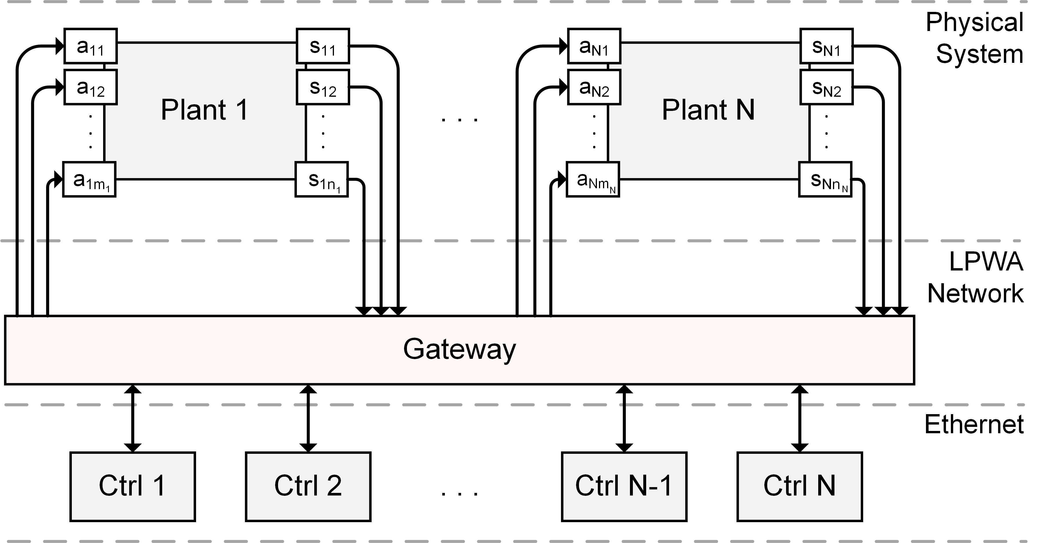
Figure 1. The architecture of WA-CPS.

Physical System and Controller. A WA-CPS physical system consists of $N$ subsystems each labelled $i$, where $i\in\{1,\ldots,N\}$. Each subsystem consists of a single plant and a single controller, and both are labelled with the same $i$ as their subsystem. We describe the $i$th subsystem’s plant using a linear time-invariant model:

(1) $$\dot{\xi_{i}}(t)=A_{i}\xi_{i}(t)+B_{i}v_{i}(t).$$

The vectors $\xi_{i}(t)\in\mathrm{R}^{n_{i}}$ and $v_{i}(t)\in\mathrm{R}^{m_{i}}$ are the state and control input vectors of subsystem $i$, respectively. $n_{i}$ and $m_{i}$ correspond to the number of sensors and actuators of the subsystem $i$, respectively. $A_{i}$ and $B_{i}$ are the matrices appropriate to the application.

The plant $i$ is instrumented with sensors $\{s_{i1},s_{i2},\ldots,s_{in_{i}}\}$ to measure its physical processes (individual states of $\xi_{i}(t)$). The controller receives these measurements and processes them according to an underlying control scheme. The goal of the controller is to maintain the values in vector $\xi_{i}(t)$ in Eq. 1 at a certain fixed value, a reference or set-point. We use a linear input-to-state feedback controller given as:

(2) $$v_{i}(t)=K_{i}\hat{\xi_{i}}(t),$$

where $\hat{\xi_{i}}(t)\in\mathrm{R}^{n_{i}}$ are the measured values of states transmitted to the controller. $K_{i}$ is a designed control gain for which the closed-loop matrix $A_{i}+B_{i}K_{i}$ is a Hurwitz matrix.

The output of the controller is an action that is sent to actuators $\{a_{i1},a_{i2},\ldots,a_{im_{i}}\}$ to influence the dynamics of the plant. The communication between the plant and the controller forms a single feedback control loop and spans potentially kilometres.

The feedback control loops in WA-CPS systems have dynamics where changes occur on the order of tens of seconds rather than milliseconds. We use a two-step process to engineer a controller that can achieve and maintain the stable operation of a subsystem. First, we design the control gain $K_{i}$ in Eq. 2 so that the controller has a slow response to system changes. The slow response reduces the overshoot (deviation from the reference or set-point) of the system’s state. Second, we choose an event-based control system because it minimises the overall number of data transmissions, saving bandwidth, which are requirements of our LPWA networks. We present the definition of event-based control in Sec. 4. The set of parameters that guarantee the stability of the subsystem $i$ (based on the Corollary 4.1 in Sec. 4.3) are:

• Sampling interval, $h_{i}$ - The time between individual samples. We address systems whose dynamics change slowly. The sampling time supported by the controller is in the order of tens of seconds (from $1$ to $50$ seconds).

• Maximum allowable transmission delay, ${\tau_{d}}_{i}$ - The maximum interval between sensor node state measurement and the time the actuator nodes receive updated controller actions. The delay supported by the $C^{3}$ approach is in the order of seconds (from $0$ to $15$ seconds).

• Event trigger parameter, $\sigma_{i}$ - It defines the size of the error between the estimated and measured states. A small $\sigma_{i}$ is more sensitive to change and triggers new control inputs at a faster rate which leads to a larger number of events. We chose to use the largest $\sigma_{i}$ that can still guarantee stable system operation to minimise energy consumption.

• Convergence rate of the control system, $\rho_{i}$ - WA-CPSs do not have strict restrictions on convergence speed as long as they can meet the delay tolerances, hence $\rho_{i}=0.001$ for all $i$.

These parameters are core to our $C^{3}$ approach as they are shared with and influence the communication system behaviours described next.

In this work, we assume that sensor nodes and actuator nodes are not collocated. We assume that all of the sensors are low-power embedded devices and battery-powered (either primary or secondary batteries). Actuators are battery or mains powered when the actuation function requires relatively high power. However, our approach is directly applicable to wireless networks where the sensors and the actuators harvest energy for energy-neutral operation, which is relatively deterministic and appropriate (Dicken et al., 2012).
Wireless Communication System. We focus on LPWA networks because they are designed as low-power one-hop wireless solutions for long-distance communication. LPWANs enable communication between the sensors, the actuators, and the controller over multi-kilometre distances. Single-hop wireless networks are better than multi-hop wireless networks for control-based systems due to their increased reliability and lower (easier to determine) communication delays (Lu et al., 2016; Vilajosana et al., 2019).

All $N$ subsystems in Fig. 1, and therefore $N$ feedback control loops, are coupled through the shared LPWA communication network and use a single gateway. We use the term gateway and controller interchangeably and treat them as one device. The gateway and the controllers communicate via wired communication which is instantaneous and reliable. In practice, the controller and gateway may reside on different devices, the controller on a server along with other processes (logging and management) and the gateway in a position favourable to receive radio communication (on a rooftop).

We assume that packet loss occurs only as a result of message collisions when two packets arrive at the same time. Sensors always send up-to-date information and retransmit if no acknowledgement is received. If information is delayed due to retransmission and a new message is generated, the original information is replaced by the most up-to-date information.

We specify the parameters of the LPWA network that affect the function of the network and the controller:

• Channel access time, $t_{ca}$ - The maximum time that a sensor node takes to access the channel to send, dependant on the channel access scheme used. The goal of our $C^{3}$ approach is to minimise $t_{ca}$ and any other waiting times (delays) due to the time-criticality of information in controlled systems.

• Time to complete the transmission, $t_{t}$ - The maximum time that it will take for a sensor node to transmit its data to the controller (assuming it accessed the channel beforehand) and for the controller to update and transmit its action to an actuator node. We assume reliable communication, so a lost packet triggers a resend. If newer information is available on the sensor node, then the old information is replaced by the newer information for sending.

• Duty cycle, $DC$ - The maximum percentage of time spent in communication per node per channel for a given time interval. For instance, a 1% duty cycle allows a sensor node to send for 1 second out of every 100 seconds. We assume that any communication network that we use will have a fair use policy enforced on the system to allow multiple users.

In the next section we will discuss how the key parameters for the control system and communication system influence each other. The design of the system by the selection of their values is the core of our $C^{3}$ approach.

2.2. Co-design Constraints

$C^{3}$ maps an event-based control scheme to a LPWA protocol, and vice versa, through their coupled parameters. The set of key design parameters from the event-based controller is $\{h_{i},{\tau_{d}}_{i},\sigma_{i},\rho_{i}\}$ and the parameters for the communication are $\{t_{ca},t_{t},DC\}$. The coupling between two sets of parameters is twofold and given via two co-design constraints. These are:

1. The control parameter ${\tau_{d}}_{i}$ is directly affected by the communication parameters: $t_{ca}$, $t_{t}$ and $DC$. The stability can be guaranteed (based on Corollary 4.1 in Sec. 4.3) only if the service time for each event is less than ${\tau_{d}}_{i}$ ($0$ to $15$ seconds) while complying with the $DC$ restriction. We define the service time as the sum of delays due to $t_{ca}$ and $t_{t}$.

2. The choice of control parameters $h_{i}$, $\sigma_{i}$ and $\rho_{i}$ determine the number of events which cause transmissions. These constitute the load on the communication network. The network load cannot be larger than the maximum network capacity. Again, the choice of these parameters is dependant upon C₁, and stability has to be guaranteed (based on Corollary 4.1 in Sec. 4.3).

Our $C^{3}$ approach focuses upon these co-design constraints to enable the design of the WA-CPS. The next two sections will focus on the two sides of our $C^{3}$ approach separately. First, we focus upon the design of a communication protocol for WA-CPSs, then we look at the design of a controller for WA-CPSs. We show how the use of $C^{3}$ ensures that the resulting communication and control systems meet the above co-design constraints and guarantee stability.

3. An LPWA Communication Infrastructure for Control

In this section, we present a novel LPWA MAC protocol called Ctrl-MAC. Ctrl-MAC is the result of the application of our $C^{3}$ approach and is agnostic to specific LPWA technologies such as LoRa, NB-IoT or Sigfox (Raza et al., 2017). First, we present the operating principle and the implementation details of Ctrl-MAC. Then, we present a delay analysis to show that Ctrl-MAC bounds communication delays and adds guarantees to the low data rates and unreliable communication typical of all of the current, major LPWA technologies. In doing this, Ctrl-MAC ensures that the communication requirement of control systems (the co-design constraint C₁) is met. Finally, we evaluate Ctrl-MAC against LoRaWAN, a state-of-art LPWA MAC protocol. Our results confirm that Ctrl-MAC achieves lower, bounded communication delays, reliable two-way communication and higher throughput when compared to LoRaWAN.

3.1. Ctrl-MAC Operating Principle

Ctrl-MAC operates in two phases: (1) Sensing and data transmission phase (2) Control update and actuation phase. These are given next.
Phase 1: Sensing and Data Transmission. In the sensing and data transmission phase, each sensor node (within each subsystem) goes through three stages.

The first stage is when the sensor node senses the physical phenomenon. This data is interrogated to identify if a significant event has occurred. It is transmitted if a significant event is identified. The sensor sleeps until the next sensing period if no significant event is identified.

Upon the identification of an event, the sensor synchronises to the start of the request period. The sensor updates its local device clock to the start time of a request reply message (RRM, shown in Fig. 2) received from the gateway. The gateway sends RRMs periodically. Synchronisation is required to correct the clock drift caused after the sensor node resumes from power-saving deep sleep mode. The sensor node also learns the number of request slots $k$, the duration of each request slot $t_{slot}$ from the RRM.

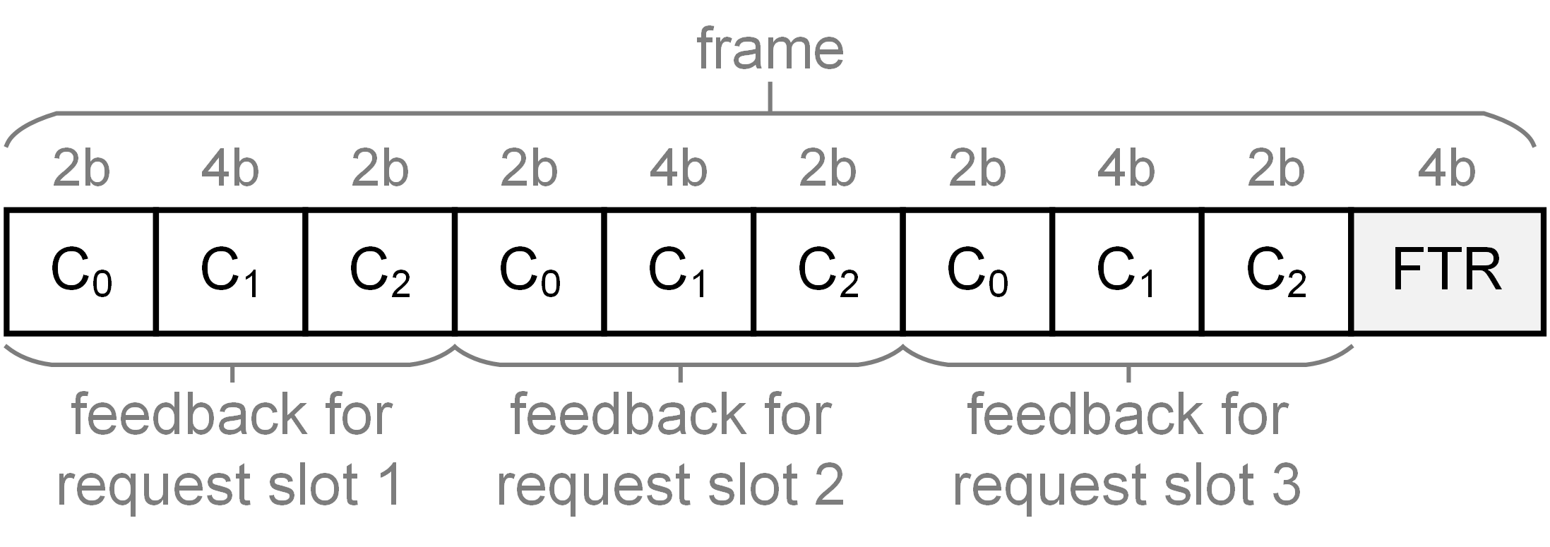
Figure 2. The RRM structure for $k=3$, $M_{D}=3$ which implies that $size(C_{2})$=$\log_{2}{M_{D}}$, $l=16$.

The second stage is when the sensor node transmits its data transmission request. Once the sensor node is synchronised to the request period, it randomly chooses which slot to transmit in. The sensor chooses using a uniform random distribution of all available request slots instead of a fixed slot or following a round-robin slot scheduling scheme. This is done to manage the case where there are more sensor nodes than available request slots where no fixed schedule is possible. The sensor makes a data transmission request by transmitting its ID during its chosen time slot. If the sensor is the only one requesting a transmission slot, its request will be successful; otherwise, there will be a collision (a result of slot contention) and the request for both sensors will fail.

The sensor node is informed about the success or failure of its data transmission request in the next RRM. An example of a RRM for a system with $k=3$ transmission request slots and $l=16$ data slots is shown in Fig. 2. The RRM contains three fields for each transmission request slot. These are:

1. The state of the request slot, $C_{0}\in\{0,1,2\}$, where $C_{0}=0$ indicates that no sensor node sent a request in this request slot, $C_{0}=1$ indicates that there was no contention in this request slot and $C_{0}=2$ indicates that a collision occurred in this request slot.

2. The data slot counter, $C_{1}\in\{1,\ldots,l\}$, where $l$ is the number of data slots.

3. The data channel counter, $C_{2}\in\{1,\ldots,M_{D}\}$, where $M_{D}=M-2$ is the number of data channels and $M$ is the overall number of channels.

The last value of an RRM is called the $FTR$. $FTR$ contains the cumulative sum of all contentions that have not been resolved until now. This includes the current failed and previous failed transmission requests. The $FTR$ is decremented by $1$ after each RRM.

A sensor node checks the value of $C_{0}$ in the request slot that it used to transmit its data transmission request. If $C_{0}=1$, that sensor node can proceed to stage three and send data. If $C_{0}=2$ the data transmission request fails. The sensor node must return to stage two and send another transmission request at the time defined by the value of $FTR$. If $FTR>1$, the sensor node counts all of the other request slots that have $C_{0}$ equal to $2$. This value is denoted as $r$. The sensor node determines the position of its request slot compared to other $r-1$ request slots. This value is denoted as $p$. The sensor node waits for the $(FTR+r-p)$th RRM to retransmit its data transmission request choosing the slot $k$ randomly.

In stage three, the sensor node transmits data. The RRM contains information to partition data transmissions into $(M-2)$ channels and $l$ data slots. The gateway allocates channel/slot pairs to requesting sensors on a first-come-first-served basis. When a sensor node receives an RRM with $C_{0}=1$ it changes to the channel given in $C_{2}$ and transmits its data in the slot given by $C_{1}$. If the sensor node senses new data during the time that it is requesting a transmission slot, it will send the new data, and discard the old. This is because the controller requires the newest information to keep the system stable.
Phase 2: Control Update and Actuation. The second phase of Ctrl-MAC is the control and actuation phase. After the controller receives sampled information from the sensor node, it uses it to calculate the control action that should be sent downstream to actuator nodes. This constitutes one of the challenges met by our co-design approach. Current LPWA protocols such as LoRa and NB-IoT prioritise upstream communication only and are therefore ill-suited to meet the timing requirements of control systems with feedback loops. Instead, Ctrl-MAC adds bidirectional capability to current LPWA protocols where the downstream communication is as important as the upstream communication.

The gateway sends actuation information to the actuator nodes in the downlink message. These messages are sent periodically so no $DC$ regulations are violated. The size of each downlink message can change depending on how many actuator nodes need to be updated. The sending time of this message will depend on the size of the previous downlink message (such that it complies with the DC regulation).

Next, we give the details of the Ctrl-MAC implementation and design choices.

3.2. Ctrl-MAC Implementation

We implemented Ctrl-MAC as a proof of concept on top of LoRa. We use LoRa’s physical layer because it is robust, has open-source libraries and uses inexpensive low-powered hardware. LoRa operates in the unlicensed spectrum and is subject to fair usage policies mandated by legislation. Fair usage takes the form of a self-imposed DC of 1% and 10% time-on-air for transmissions when operating in the EU region. As Ctrl-MAC is implemented on top of LoRaPHY, it is important that we explain our motivation for not using LoRaWAN, a LoRa MAC protocol, and the differences between the two. These are given in Sec. 3.4. Our reference implementation of Ctrl-MAC has room for significant performance improvement. It purposefully does not exploit any LoRa performance enhancing features, such as the use of different spreading factors, to be general to LPWA communication schemes such as NB-IoT or SigFox. Further, in all simulations and experiments Ctrl-MAC maintains a constant spreading factor of 7 which gives low transmission time and achieves distances of up to $2$km (Adelantado et al., 2017) in urban areas.

Ctrl-MAC assumes that there are four channels available based on the EU recommendation (Committee, 2018). There are three uplink channels of $125$kHz with $1$% DC and one downlink channel of $250$kHz with $10$% DC. The current LoRaWAN implementation uses only half ($125$kHz) of the allocated downlink bandwidth for the acknowledgements. Ctrl-MAC exploits this feature and uses the remaining $125$kHz to send the actuation signals to actuator nodes. The actuation signals are periodically transmitted while complying with the 10% DC regulation. The size of the downlink message depends on the number of actuator nodes in the network and how many bytes of information are used per an actuator. For example, for a network with $10$ actuator nodes and $2$Bytes of information with the 10% DC regulation, the actuation messages can be transmitted every $0.5$ seconds.

Our implementation uses only a single channel for data request transmissions (with 10% DC) and the remaining three channels for data transmission. The results in Fig. 3 (left) show that when only a single channel is used for data request transmissions (with 10% DC) and the remaining three channels for data transmission, Ctrl-MAC achieves lower delays and higher packet delivery ratios (PDRs) than when all four channels are used for both. This happens because the data transmission requests and actual data transmissions operate concurrently unlike the case when the data transmission requests and actual data transmissions happen on the same channel one after the other. Our implementation allows more requests to be sent, the contention is resolved faster and data load is distributed evenly over 3 data channels, and therefore more data can be sent.

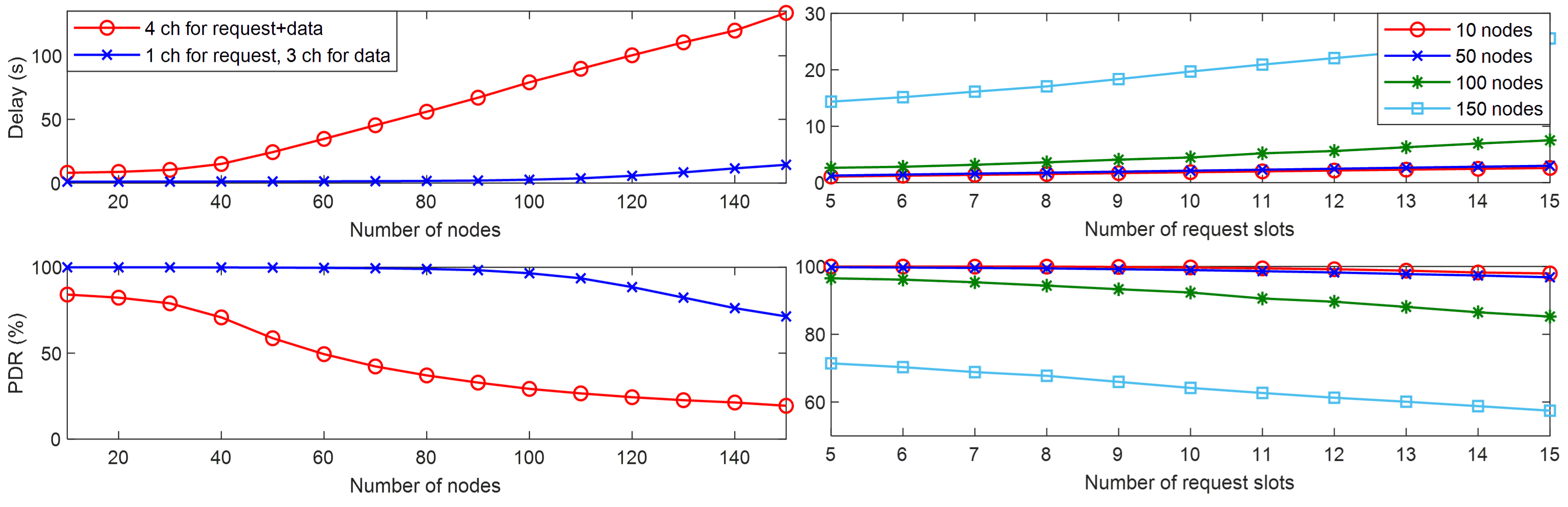
Figure 3. (left) Ctrl-MAC channel disciplines comparison, (right) Ctrl-MAC request slots comparison.

Ctrl-MAC uses $k=5$ request slots with the duration of $t_{slot}=0.1$ seconds. The value of $k$ cannot be smaller than $5$ and the request slots can not be of less time to account for the 10% DC regulation. The results in Fig. 3 (right) show the degradation of the communication delays and PDRs for all $k$ larger than 5 and all populations of sensor nodes.

Next, we model Ctrl-MAC to analyse its performance in terms of the guarantees and achieved communication delays.

3.3. Ctrl-MAC Delay Analysis

In this section we analyse the communication delays identified by the co-design constraint C₁ from Sec. 2.2, using a queue based approach. We show that the communication delays of Ctrl-MAC, due to $\{t_{ca},t_{t},DC\}$, are bounded and do not violate the maximum allowable transmission delay derived from the control system. The maximum allowable transmission delay for each subsystem $i$ is ${\tau_{d}}_{i}=\tau_{d}$, which is from $0$ to $15$ seconds. Our analysis obtains the bounds of $\{t_{ca},t_{t}\}$ by deriving the delays of different stages of Ctrl-MAC, $\{t_{sync},t_{req},t_{send},t_{update}\}$, where $t_{ca}=t_{sync}+t_{req}$ and $t_{t}=t_{send}+t_{update}$ while complying with the DC regulation. We show that Ctrl-MAC can operate within the communication constraints and keep the total delays less than the maximum allowable transmission delay (i.e. $t_{sync}+t_{req}+t_{send}+t_{update}<{\tau_{d}}$).
Sensing and Data Transmission Phase Delay. We model the delays incurred in the three stages of the Sensing and Data Transmission Phase and derive their maximum bounds.

The first stage of the first phase is the synchronisation process. This occurs when a sensor node has data to send and uses information in the RRM received from the gateway. The RRM message is sent periodically and of a fixed size such that the time on air of the message and its sending rate never violate the DC regulation. Therefore, the synchronisation process includes a fixed delay, denoted as $t_{sync}$, which is in the range $[0,t_{slot}\times k$]. In our system, $t_{sync}\in[0,0.5]$ seconds (based on the implementation in Sec. 3.2 that uses $k=5$ request slots of $t_{slot}=0.1$ seconds).

After the delay of $t_{sync}$, the sensor node needing to transmit enters the next two stages of phase one. Delays of the next two stages are denoted as $t_{req}$ and $t_{send}$. Their bounds are analysed by modelling the two stages as two queues:

• M/M/1 queue, or queue one - The second stage of the first phase is the data transmission request process. We model this process as an M/M/1 queue. We use a queue to analyse the delay, $t_{req}$, and its bounds as it allows us to reason about the occurrence of sensor events and the waiting time for a sensor node to receive a transmit slot for data communication. We define $t_{req}$ as the mean time for a sensor node to successfully request and receive a data slot and is estimated by $1/(\mu_{req}-\lambda)$ where $\lambda$ is the system load, less than or equal to the number of sensor nodes, and $\mu_{req}=ln(1/(1-e^{(-\lambda/k)}))$ is the service rate. We assume that the inter-arrival of sensor events and time to get a transmit slot are exponentially distributed (these assumptions are based on the traffic pattern of an event-based control system as presented in Sec. 4.4). For the system to be stable $\lambda/\mu_{req}<1$. The delay $t_{req}$ is non-deterministic. In the best case scenario, when the sensor node immediately successfully requests and receives a data slot $t_{req}=0.2$ seconds. Otherwise, we can analyse that the probability of $t_{req}$ is less than a given delay which we denote as $x$. We show through numerical simulation the probability $P[t_{req}\leq x]=1-e^{(-(\mu-\lambda)x)}$ for various data loads. Results are presented in Fig. 4. Our results show a very high probability (more than 99%) of meeting the delay bounds of $5$ seconds for a communication capacity of up to $136$ packets per minute and up to $150$ packets per minute of meeting the delay bounds of $10$ seconds. The packet sizes and time on air of packets at this rate do not violate the DC regulation.

• M/D/$n$ queue, or queue two - The third stage of phase one is the data transmission stage. We model the delay of this stage, $t_{send}$, as an M/D/$n$ queue. The term $n$ is the number of data transmission channels available to Ctrl-MAC. We define $t_{send}$ as the time for a sensor node to send its data to the gateway. The queue is deterministic because a sensor node receives the data slot and channel exclusively reserved for its transmission from the gateway during the data transmission request stage. The exclusive data slot and channel reservation ensure that the DC regulation is met, and that the time to send is bounded. The delay $t_{send}$ is equal to $1/n+(\lambda_{dt}/(2n\times(n-\lambda_{dt})))$ where $\lambda_{dt}$ is the output of the M/M/1 queue given above and the input to the M/D/$n$ queue described here. Based on the input rate, $\lambda_{dt}$, is in the range of $[12,150]$ packets/minute based on Fig. 4, the time to completion is $t_{send}\in[0.3,0.45]$.

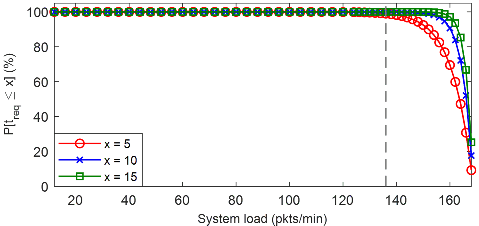
Figure 4. The probability of achieving $t_{req}\leq x$ for M/M/1 queue.

Control Update and Actuation Phase Delay. The final delay that we need to consider is the time for phase two, $t_{update}$, when the controller sends the control input to the actuator node. The gateway transmits on a separate downlink channel reserved for communication from the gateway to the actuator. The use of a reserved channel ensures that the $DC$ regulation is met and that the time of $t_{update}$ is deterministic. The delay is dependant upon the specific LPWAN technology and the size of last actuation update sent. In our LoRa implementation, the maximum packet size that the controller can send is $222$ bytes. Each actuation update is 2 bytes per actuator node, 1 byte for control input and 1 byte for addressing. The maximum number of actuator nodes that can be updated with a single packet is $111$. The delay $t_{update}$ is in the range of $[0.4,3.6]$ seconds depending on the size of the last actuation update.

Therefore, the total delay introduced by Ctrl-MAC, $t_{MAC}$ is:

(3) $$t_{MAC}=t_{sync}+t_{req}+t_{send}+t_{update}.$$

According to the co-design constraint C₁ from Sec. 2.2, the system stability is dependant upon the condition that ${\tau_{d}}>t_{ca}+t_{t}$ where $t_{ca}=t_{sync}+t_{req}$ and $t_{t}=t_{send}+t_{update}$. We derived the individual bounds for $t_{sync}$, $t_{req}$, $t_{send}$, and $t_{update}$ while taking the DC regulation into account. A simple sum of all of our bounds shows that the total delay, $t_{MAC}$ is in the range of $[0.9,14.55]$ seconds with a very high probability of more than 99%. The communication delays of Ctrl-MAC do not violate the maximum allowable transmission delay of the system (i.e. $\tau_{d}>t_{MAC}^{Upper}$).

3.4. Ctrl-MAC and LoRaWAN

In this section we motivate the need for Ctrl-MAC, we explain the differences between Ctrl-MAC and LoRaWAN, and show how LoRaWAN is unable to meet communication requirements for control systems that are reliable communication, two-way communication and bounded communication delays. We evaluate Ctrl-MAC against two versions of LoRaWAN:

• Version one: LoRaWAN - This is a baseline version that represents the typical use case for LPWA technology such as data collection from sensors or smart meters. It exploits a pure ALOHA channel access scheme. The sensor nodes are the Class A devices (Committee, 2018) which use unconfirmed (unacknowledged) messages, i.e. the sensor nodes do not request an acknowledgement for their uplink transmissions and hence there is no guarantee for successful delivery of the message. The actuator nodes are modelled as Class C devices. As mentioned in the LoRaWAN specification (Committee, 2018), Class C devices are always listening on the downlink channel unless they are transmitting data. Our actuation messages are sent on this downlink channel to the actuators.

• Version two: LoRaWAN++ - This is an improved version of LoRaWAN that enables reliable data communication to the gateway. It uses the ALOHA channel access scheme with an acknowledgement message from the gateway for every uplink transmission, as described in the LoRaWAN specification (Committee, 2018). If no acknowledgement is received, the transmitted data is resent up to $8$ times after which it is dropped. Acknowledgements are sent on the LoRaWAN downlink channel. In this version we also add a dedicated downlink channel for actuation to make this scheme comparable to Ctrl-MAC.

We evaluate MAC protocol suitability for control applications with three metrics:

1. End-to-End Packet Delivery Ratio (E2E PDR in %) - E2E PDR is the ratio of the number of unique actuation updates received by the actuator node over the number of unique events generated by the corresponding sensor node. This metric indicates the suitability of the MAC protocols for control applications in terms of two-way communication. The downstream communication is as important as upstream communication.

2. End-to-End Delay (E2E Delay in seconds) - E2E Delay is defined as the difference between the time that an actuator node receives the actuation update and the time that an event is generated at the sensor node. We assume the computation delays to be zero when calculating this metric. This metric indicates the suitability of the MAC protocols for control applications in terms of bounded communication delays.

3. Uplink Reliability (UL Reliability in %) - UL Reliability is the ratio of the number of events successfully acknowledged by the gateway over the number of events successfully delivered at the actuator nodes. This metric gives the guarantees that the controller has complete and up-to-date information to maintain system stability. For example, a 10% uplink reliability would indicate that only 10% of the delivered messages from sensor nodes were reliably acknowledged. The sensor nodes may or may not have information about the remaining 90% which introduces uncertainties in the system.

We compare the E2E PDR, E2E Delay and UL Reliability of Ctrl-MAC, LoRaWAN and LoRaWAN++ assuming four channels, a varied number of nodes (${10,50,100,150,200}$) and two transmission patterns. First, we chose constant periodic transmissions to represent the worst-case scenario of the event-triggered control (i.e. at every sampling period, the transmission is triggered - in reality there would be periods of no events). Each sensor periodically sends data with an interval of ${10,30,50}$ seconds. Second, we chose exponential transmissions with a mean of ${10,30,50}$ seconds to represent aperiodic and bursty traffic patterns specific to the event-triggered control. This range of sending rates (inter-arrival times) corresponds to the sampling interval of slow-loop control systems as it is shown in Sec. 4.4. Results are presented in Tables 1, 2 and 3.

Table 1. E2E PDR (%) of Ctrl-MAC/LoRaWAN/LoRaWAN++ under different data loads and data distributions.

	Ctrl-MAC					LoRaWAN					LoRaWAN++
Size	10	50	100	150	200	10	50	100	150	200	10	50	100	150	200
P(10s)	99.99	67.72	33.62	22.34	16.86	99.98	64.32	39.82	30.26	23.22	80.85	40.31	31.39	25.89	20.24
P(30s)	99.99	99.99	98.23	67.20	50.77	99.98	80.23	72.64	57.6	48.14	99.96	86.71	40.11	27.56	21.04
P(50s)	99.99	99.99	99.99	99.99	83.74	99.99	93.13	85.56	65.18	62.95	99.99	93.06	63.37	45.31	34.50
E(10s)	99.98	97.59	52.73	35.27	26.43	84.42	66.44	51.32	41.45	33.44	86.31	38.54	21.34	14.66	10.94
E(30s)	99.99	96.01	91.79	79.84	60.38	93.22	83.52	72.71	64.08	55.95	98.31	72.95	45.80	32.22	24.46
E(50s)	99.99	97.76	97.31	95.67	93.00	95.81	88.58	81.13	73.96	68.23	99.18	89.28	64.86	47.77	37.46
P=periodical, E=exponential

Table 2. E2E Delays (s) of Ctrl-MAC/LoRaWAN/LoRaWAN++ under different data loads and data distributions.

	Ctrl-MAC					LoRaWAN++
Size	10	50	100	150	200	10	50	100	150	200
P(10s)	1.38	9.17	23.37	37.66	52.77	4.15	14.39	15.68	15.56	14.84
P(30s)	1.28	1.48	5.85	26.31	36.02	3.32	11.92	15.26	15.60	15.40
P(50s)	1.27	1.41	1.66	2.8	25.54	0.33	8.54	14.52	15.57	15.26
E(10s)	1.35	2.81	17.29	31.96	46.65	3.58	13.41	15.52	15.63	15.03
E(30s)	1.30	1.48	2.91	14.99	27.03	1.63	9.51	14.33	15.56	15.38
E(50s)	1.29	1.37	1.59	2.45	7.73	1.16	6.36	12.28	14.62	15.46
LoRaWAN E2E Delays are 0.15 seconds for all simulation scenarios.
P=periodical, E=exponential

Table 3. UL Reliability (%) of Ctrl-MAC/LoRaWAN/LoRaWAN++ for $10$ and $200$ nodes

	P(10s)		P(30s)		P(50s)		E(10s)		E(30s)		E(50s)
Protocol	10	200	10	200	10	200	10	200	10	200	10	200
LoRaWAN	UL Reliability is 0% for all simulation scenarios.
LoRaWAN++	98.76	34.62	99.92	37.81	99.99	39.41	99.46	35.36	99.96	41.91	99.99	50.81
Ctrl-MAC	UL Reliability is 100% for all simulation scenarios.
P=periodical, E=exponential

The results clearly demonstrate that LoRaWAN is not suitable for control systems as it stands; it was not designed for this. It achieves very low E2E PDRs (less than 90%), except in the case of very small network sizes and low data rates. This implies failing to support two-way communication. LoRaWAN does not support acknowledgement messages which prevents reliable data transmission to the gateway. The E2E Delays are constant and low as LoRaWAN uses pure ALOHA. This implies that any contention-free transmission will have same E2E delays which would be a sum of the uplink and downlink time on airs which equals 0.15 seconds; however, the percentages of contention-free transmissions are very low as per Table 1. Stable controlled system operation that we derive in Sec. 4.3 can not be guaranteed as it is shown in (Tomić et al., 2018) with LoRaWAN.

Similar to LoRaWAN, LoRaWAN++ is also unable to meet the communication requirements for wide area control systems. LoRaWAN++ achieves good E2E PDRs (more than 90%) for small network sizes and low data rates. However, for larger network sizes and higher data rates, there is a network performance deterioration; E2E PDRs are even lower than in the case of LoRaWAN. These results align with the results in (Pop et al., 2018) which show that if 100% of the nodes request an acknowledgement, the network can barely operate at 15% of its capacity compared to the scenario when no-one requests an acknowledgement. LoRaWAN++ E2E Delays are always less than $20$ seconds as it allows $8$ retransmissions, after which the packet is dropped. This means that LoRaWAN++ can provide guarantees of bounded communication delays. However, it fails to guarantee reliable and two-way communication. Not all delivered messages are acknowledged (based on the results in Table 3) and this discrepancy increases with the number of nodes adding uncertainty to a closed-loop system.

Finally, the results show that Ctrl-MAC is able to meet all communication requirements for control systems for the networks of up to 150 nodes with a maximum data rate of 1 packet per 50 seconds. Higher rates can be supported for the networks with less than 150 nodes (see Table 1). This practical limitation of Ctrl-MAC for networks larger than 150 nodes per gateway is reasonable and as per general LoRa recommendations. To increase the scale of such a single-hop network one would include more gateways to have gateway diversity rather than trying to handle more nodes per gateway. Ctrl-MAC achieves high E2E PDRs for a much larger number of scenarios when compared to LoRaWAN and LoRaWAN++. It achieves bounded E2E Delays and is also able to guarantee UL reliability of 100% for all simulated scenarios. This UL reliability can be guaranteed because all data transmissions are scheduled; hence, there is no possibility of data collisions.

4. Control Model for a Water Distribution Network

In this section, we present a system model for our large-infrastructure reference example, a water distribution network. We demonstrate how we use our $C^{3}$ approach to influence the controller design to meet the co-design constraint C₂ in Sec. 2.2 and enable safe and reliable system operation. The communication requirements of the controller (based on the choice of $\{h_{i},{\tau_{d}}_{i},\sigma_{i},\rho_{i}\}$) cannot be larger than the maximum communication network capacity. At the same time, the parameters $\{h_{i},{\tau_{d}}_{i},\sigma_{i},\rho_{i}\}$ have to be chosen such they guarantee the system stability.

4.1. System Model & Controller Design

The water distribution network model considered in this paper is shown in Fig. 5.

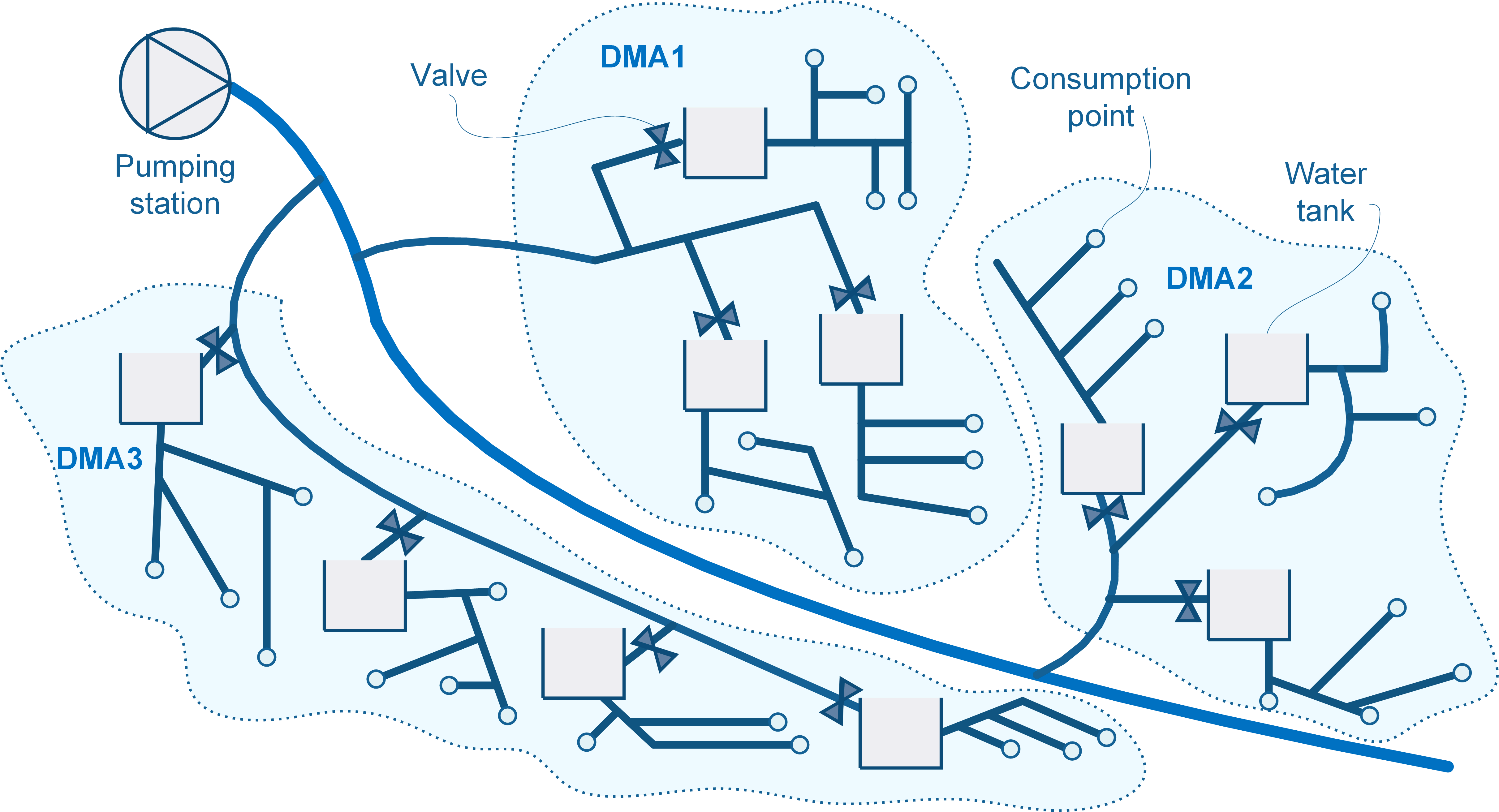
Figure 5. The water distribution network.

It consists of several District Meter Areas (DMAs). Each DMA has three or four water tanks that supply on average $10$-$30$ customer connections via a set of pressurised pipes, pumping stations, and valves. Their dynamics are complex, non-linear, difficult to model and analyse. If the complexity of the water network is reduced to a problem of stabilising the tank water level to a pre-defined set point, the non-linear model can be linearised as in (Kartakis et al., 2018).

Each DMA (or plant, in general terms) is instrumented with $n_{i}$ sensor nodes (for measuring the water level in the tanks) and $m_{i}$ valves for actuation. Each DMA is modelled by the linear time-invariant model in Eq. 1. In the state vector $\xi_{i}(t)$, each state is the difference between the current water level and set point reference water level for a tank. The control input vector $v_{i}(t)$ represents the degree to which the in-valves are open to fill each tank.

The system states are measured with water level sensor nodes for each DMA supply tank. The states are communicated to the linear input-to-state controller given in Eq. 2. The values in $\hat{\xi}_{i}(t)$ contain either the previous measured values or new measured values of $\xi_{i}(t)$. A new measured value for a tank is used if the measured value violates the event condition (defined in next section). Otherwise, the previous measurement of the water level in the DMA tanks is used. The combination of previous and new values creates an estimation of $\xi_{i}(t)$. The error, or difference, between the estimated levels and the measured levels is

(4) $$\varepsilon_{i}(t)=\hat{\xi}_{i}(t)-\xi_{i}(t).$$

From a control system point of view, we can view the water tank levels in $\xi_{i}(t)$ as those on the sensor nodes, and the values in $\hat{\xi}_{i}(t)$ as the values on the controller.

It is the task of Ctrl-MAC to send the new values from the sensors to the controller when required. We refer to this process as the sample-and-update of $\xi_{i}(t)$. The speed at which updates occur determines the system stability and the congestion of the communication network which relates to the co-design constraint C₂. The speed is regulated by the update mechanism given next.

4.2. Updating the Control Input

The traditional way of choosing when to update $\hat{\xi}_{i}(t)$ is periodic, or Time-Triggered Control (TTC). In TTC all of the sensors send updates at a fixed interval. This method wastes energy when no changes to the water levels warrant sending and can cause network congestion. Instead, we focus on Decentralised Periodic Event-Triggered Control (DPETC) from (Heemels et al., 2013). DPETC reduces both the communication from the sensor nodes to the controllers and the energy consumption of the sensor nodes (Kartakis et al., 2018).

We summarise DPETC from (Heemels et al., 2013) with modifications for our input-to-state feedback control system (to accommodate the co-design constraint C₂). The equation

(5) $$\mathcal{T}_{k}:=\{t_{k}|t_{k}:=kh,k\in\mathbb{N}\}$$

denotes the periodic sampling sequence of the sensor nodes in time. The term $h>0$ is the time between samples and $k$ is the sample number. The sensor $s_{ij}$ of DMA $i$, where $j\in\{1,\ldots,n_{i}\}$ updates its state, $\hat{\xi}_{ij}(t)$, on the controller as

(6) $$\hat{\xi}_{ij}(t)=\left\{\begin{aligned} &\xi_{ij}(t_{k}),\,\text{when }\mathcal{C}_{ij}(\xi_{ij}(t_{k}),\hat{\xi}_{ij}(t_{k}))>0\\ &\hat{\xi}_{ij}(t_{k}),\,\text{when }\mathcal{C}_{ij}(\xi_{ij}(t_{k}),\hat{\xi}_{ij}(t_{k}))\leq 0\end{aligned}\right.$$

for times $t\in(t_{k},t_{k+1}]$. The quadratic event-trigger condition $\mathcal{C}_{ij}(\xi_{ij}(t),\hat{\xi}_{ij}(t))$ defines when there is an event and a sensor needs to send its value ($\xi_{ij}(t)$) to update $\hat{\xi}_{ij}(t)$. The event condition $\mathcal{C}_{ij}$ is

(7) $$\mathcal{C}_{ij}(\xi_{ij}(t),\hat{\xi}_{ij}(t))=|\hat{\xi}_{ij}(t)-\xi_{ij}(t)|-\sigma_{ij}|\xi_{ij}(t)|.$$

Based on Eq. 7, small $\sigma_{ij}$ triggers new events faster which for us means that the load to our communication network will be higher. With this in mind, we choose to use a $\sigma_{ij}$ that triggers the least number of events but still guarantees stable system operation as per the co-design constraint C₂. In doing so, we perform stability analysis for our DPETC based on (Borgers et al., 2018). The goal of the analysis is to define the maximum allowable delay $\tau_{d}$ and $\sigma_{ij}=\sigma$ for all $i$, for which the control system is stable. The stability analysis is presented next.

For our stability analysis, we define $\mathcal{J}$ to be a set that contains the states transmitted at time $t_{k}$ and $\mathcal{J}_{c}$ to be a set of the states not transmitted at time $t_{k}$. We define $\Gamma_{j}$ as a diagonal matrix where the $j$th diagonal element equals $1$ and the rest of diagonal elements equal $0$.

4.3. Stability Analysis

The following stability analysis determines the maximum allowable delay $\tau_{d}$ for the chosen values of $h$, $\sigma$ and $\rho$ that renders the controlled system stable. Please note that we dropped denoting subsystems by $i$ for the sake of clarity. However, the analysis refers to an individual subsystem (or DMA) given in Eq. 1 and its controller in Eq. 2.

The condition for having a globally exponentially stable (GES) system is that there exist scalars $c>0$ and $\rho>0$ such that for all $\xi(0)\in\mathbb{R}^{n_{s}}$ for all $t\in\mathbb{R}^{+}$ the following holds: $|\xi(t)|\leq ce^{-\rho t}|\xi(0)|$. The stability proof follows from the Corollary III.3 and Theorem V.2 of (Heemels et al., 2013), and Theorem IV.1 of (Borgers et al., 2018) and it is briefly summarised in the following corollary.

Corollary 4.1.

Consider plant in Eq. 1, controller in Eq. 2, sampling sequence in Eq. 5, event-triggered mechanism in Eq. 6, and event-triggered condition in Eq. 7. Let $\tau_{d}$ be a given maximum allowable delay and $\rho$ be a given convergence rate. Assume there exist matrices $P_{0h}\succ 0$ and $P_{1d}\succ 0$, and scalars $\acute{\mu}_{\mathcal{J}}^{j}\geq 0$, $\acute{\mu}_{\mathcal{J}_{c}}^{j}\geq 0$, $\tilde{\mu}_{\mathcal{J}}^{j}\geq 0$, $\tilde{\mu}_{\mathcal{J}_{c}}^{j}\geq 0$, $\hat{\mu}_{\mathcal{J}}^{j}\geq 0$, $\hat{\mu}_{\mathcal{J}_{c}}^{j}\geq 0$, where $j\in\{1,\cdots,n_{s}\}$, such that

(8) $$\begin{bmatrix}e^{-2\rho\tau_{d}}P_{0h}+G_{1}&\acute{J}_{\mathcal{J}}^{\mathrm{T}}e^{\bar{A}^{\mathrm{T}}\tau_{d}}P_{1d}\\ (\acute{J}_{\mathcal{J}}^{\mathrm{T}}e^{\bar{A}^{\mathrm{T}}\tau_{d}}P_{1d})^{\mathrm{T}}&P_{1d}\\ \end{bmatrix} \succ 0$$

$$\begin{bmatrix}e^{-2\rho(h-\tau_{d})}P_{1d}+G_{2}&\tilde{J}_{\mathcal{J}}^{\mathrm{T}}e^{\bar{A}^{\mathrm{T}}(h-\tau_{d})}P_{0h}\\ (\tilde{J}_{\mathcal{J}}^{\mathrm{T}}e^{\bar{A}^{\mathrm{T}}(h-\tau_{d})}P_{0h})^{\mathrm{T}}&P_{0h}\\ \end{bmatrix} \succ 0$$

where $G_{1}=\sum_{j\in\{1,\cdots,n_{s}\}}(-\acute{\mu}_{\mathcal{J}}^{j}\acute{Q}_{j}+\acute{\mu}_{\mathcal{J}_{c}}^{j}\acute{Q}_{j}-\tilde{\mu}_{\mathcal{J}}^{j}\tilde{Q}_{j}+\tilde{\mu}_{\mathcal{J}_{c}}^{j}\tilde{Q}_{j})$, $G_{2}=\sum_{j\in\{1,\cdots,n_{s}\}}(-\hat{\mu}_{\mathcal{J}}^{j}\hat{Q}_{j}+\hat{\mu}_{\mathcal{J}_{c}}^{j}\hat{Q}_{j})$ and

$$\bar{A}=\begin{bmatrix}A&BK&0\\ 0&0&0\\ 0&0&0\\ \end{bmatrix}\acute{Q}_{j}=\begin{bmatrix}(1-\sigma^{2})\Gamma_{j}&0&-\Gamma_{j}\\ 0&0&0\\ -\Gamma_{j}&0&\Gamma_{j}\\ \end{bmatrix}$$

$$\tilde{Q}_{j}=\begin{bmatrix}(1-\sigma^{2})\Gamma_{j}&-\Gamma_{j}&0\\ -\Gamma_{j}&\Gamma_{j}&0\\ 0&0&0\\ \end{bmatrix}\hat{Q}_{j}=\begin{bmatrix}0&0&0\\ 0&\Gamma_{j}&-\Gamma_{j}\\ 0&-\Gamma_{j}&(1-\sigma^{2})\Gamma_{j}\\ \end{bmatrix}$$

$$\acute{J}_{\mathcal{J}}=\begin{bmatrix}I&0&0\\ 0&I&0\\ \Gamma_{\mathcal{J}}&0&I-\Gamma_{\mathcal{J}}\\ \end{bmatrix}\tilde{J}_{\mathcal{J}}=\begin{bmatrix}I&0&0\\ 0&I-\Gamma_{\mathcal{J}}&\Gamma_{\mathcal{J}}\\ 0&0&I\\ \end{bmatrix}$$

Then, the system is GES with decay rate $\rho$.

The proof of Corollary 4.1 is given in Appendix A.1. Based on Corollary 4.1 and its proof, the feasible solution of Eq. 8 for our water distribution network can be found when $h\in[1,50]$ seconds, $\tau_{d}\in[0,15]$ seconds and $\sigma\in[0.01,0.3]$. We chose the set of parameters that guarantees stable system operation and also meets the co-design constraint C₂. It ensures that the network load is less than the maximum network capacity which we show next.

4.4. System Operation

We demonstrate the start and steady-state (or the system’s response) of our model water distribution network in Fig. 6 (left).

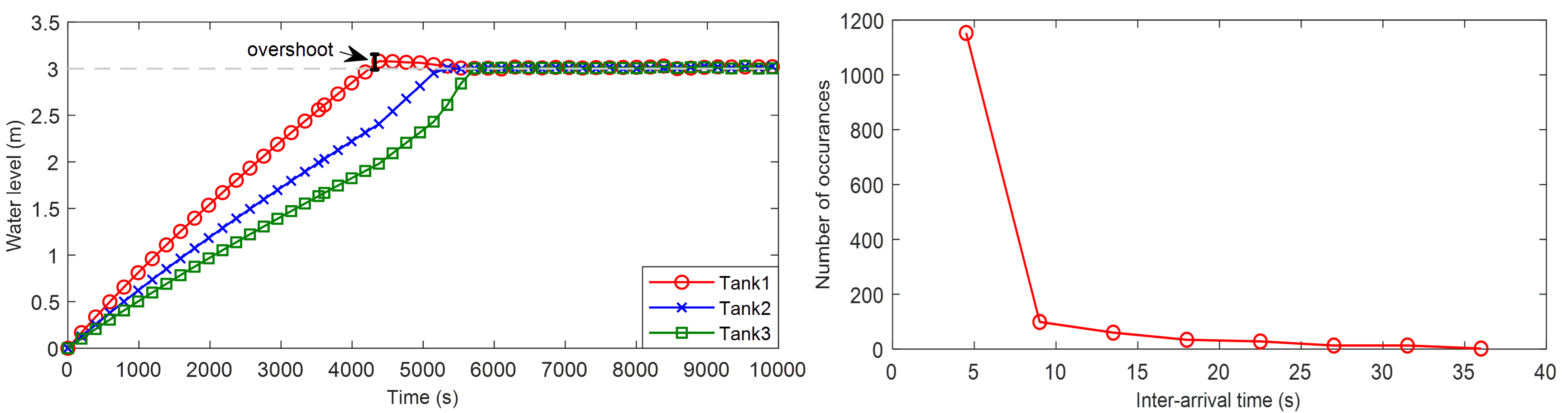
Figure 6. (left) System response to constant customer demand, (right) Distribution of inter-arrival times of the events.

The model is implemented and simulated using Matlab/Simulink, the Simscape toolbox and the Fluids toolbox. The parameters of the physical components of the DMA (pipes diameters, valve types, tank sizes) are taken from the specification sheets of the same make and model valves, pumps, and tanks as those used by water companies.

We simulate an ideal case scenario with one DMA (with three tanks) and no packet drops or delays. The control system parameters we use are sampling time of $h=4.5$ seconds and the event trigger parameter of $\sigma=0.01$. $\sigma$ regulates the rate at which events occur. For example, $\sigma=0.01$ leads to an average of $22.36$ events per minute and increasing it to $0.1$ reduces the event rate to $13.87$ events per minute. The event rate for both cases (which is the load to the communication network) is much less than the network capacity of $136$ packets/minute which is needed to ensure that the delays are bounded within a given threshold. This is presented in detail in Sec. 3.3. Therefore, our control design meets the co-design constraint C₂.

We then plot the number of occurrences of the inter-arrival times as shown in Fig. 6 (right). By using the curve-fitting toolbox, this inter-arrival times can be approximated to an exponential distribution with a mean of $4.5$ seconds (equivalent to sampling time). This supports our claim in choosing the M/M/1 queue with exponentially distributed inter-arrival times to model the input operation of Ctrl-MAC. Additionally, multiple exponentially distributed event traces (as in the case of more than one DMA) models aperiodic and bursty traffic (Chandrasekaran, 2006) which is the reality of event-based systems. In the next section, we evaluate the performance of our controller and communication protocol, or system, that we design using our $C^{3}$ approach.

5. Evaluation

In this section, we evaluate a system designed using our $C^{3}$ approach that consists of a controller and communication protocol. We refer to Ctrl-MAC and its associated controller as the $C^{3}$ system. The evaluation is based on a co-simulation environment and real-world experiments. We measure four system parameters to evaluate the success of the $C^{3}$ system with respect to the co-design constraints defined in Sec. 2.2. The parameters are:

• End-to-End Delay (E2E Delay in seconds) - The time that starts when a sensor node senses an event and ends when the actuation update is successfully delivered to the actuator. This metric measures the success of the constraint C₁.

• End-to-End Packet Delivery Ratio (E2E PDR in %) - The number of event messages received at the actuator over the number of messages generated by the sensor. For Ctrl-MAC this metric measures the success of the contention resolution and successful actuation updates and this relates to the constraint C₁.

• System overshoot percentage (OvSh in %) - The percentage of the overshoot above the reference value. It is calculated as the difference between the absolute value and reference value of the water level divided by the reference value. We use this metric to describe the stability of our system that has to hold in both constraints, C₁ and C₂.

• Average number of events per minute (Events/minute) - The average number of events per minute, measures the system load per minute. The more events, the more communication Ctrl-MAC needs to handle. This metric measures the success of the constraint C₂.

We measure these parameters for various sampling intervals, $h$, and different event trigger parameters $\sigma$ as defined in Sec. 2.1. We vary the size of the system, including different numbers of DMAs and sensor nodes. We conduct co-simulation and compare our results with real-world experiments to verify the success of the $C^{3}$ system. In the following sections we present our experiments and discuss the results.

5.1. Evaluation via Co-Simulation

We perform the first stage of the evaluation of the $C^{3}$ system on a custom co-simulation environment. This environment consists of a physical system simulator using MATLAB/Simulink and a communication simulator using the OMNeT++ network simulator. We run both Matlab and OMNeT++ on the same computer. We enable inter-process communication between Matlab and OMNeT++ using UDP.

We compare our approach to a wired centralised network and LoRaWAN++ in the co-simulation environment. The wired network represents the best-case scenario of a periodic centralised controller with no packet drops or transmission delays. LoRaWAN++ uses the ALOHA contention scheme with acknowledgement messages and a retry limit of $8$ messages. This is the only configuration of LoRaWAN that can provide partial guarantees in message delivery required by control applications, as mentioned in Sec. 3.4. We use a spreading factor of $7$ and the default $4$ channels specified in the LoRaWAN specification. We simulate the network with 3 DMAs and 10 sensor and actuator nodes. The goal of the control system is to maintain the DMA tank water levels to a reference point of $3$m as the time evolves. With the definition of overshoot percentage given above, a $4.5$m high water tank with a $3$m reference point overflows, or critically fails, with an overshoot above $50\%$. The customer demand is expressed as the degree that the out-valve of the tank is open. The maximum is 100%, and the minimum, 0%, is when the valve is closed.
Study 1: Matching Constant Customer Demand. In this co-simulation, we keep the customer demand constant at 100%. All experiments were run for $9000$ seconds.

The results in Table 4 show that the $C^{3}$ system and LoRaWAN++ both maintain the stability of the system with similar overshoots. It is because both Ctrl-MAC and LoRaWAN++ always send the latest reading, and discard any messages that were not sent successfully. However, the E2E PDR of Ctrl-MAC is on average 30% higher, and more consistent than the E2E PDR of LoRaWAN++. The E2E Delays was bounded in all cases below 2.2 seconds for Ctrl-MAC. The LoRaWAN++ E2E Delays are on average greater than 6 seconds. With the $C^{3}$ system the events/minute are always less than $136$ packets/minute, indicating that the co-design constraint C₂ from Sec. 2.2 is being met, and the network load remains within the network capacity.

Table 4. The evaluation of the $C^{3}$ system for constant customer demand in comparison with an idealistic wired control and LoRaWAN++ for control.

$C^{3}$ system	Events/minute	OvSh (%)	E2E PDR (%)	E2E Delay (s)
$h=1$s, $\sigma=0.1$	113.15	20.59	77.33	1.849
$h=4.5$s, $\sigma=0.01$	61.17	32.11	87.03	2.161
$h=4.5$s, $\sigma=0.1$	40.32	3.1	88.74	2.194
$h=4.5$s, $\sigma=0.3$	22.56	4.39	88.01	1.861
$h=10$s, $\sigma=0.1$	14.91	16.25	89.27	1.919
Wired Control	Events/minute	OvSh (%)	E2E PDR (%)	E2E Delay (s)
$h=-1$s*	$\inf$	2.73	100	0
$h=1$s	600	2.73	100	0
$h=4.5$s	133.33	2.75	100	0
$h=10$s	60	2.75	100	0
LoRaWAN++	Events/minute	OvSh (%)	E2E PDR (%)	E2E Delay (s)
$h=1$s, $\sigma=0.1$	115.8	3.15	31.4	6.143
$h=4.5$s, $\sigma=0.01$	63.35	29.04	51.04	9.859
$h=4.5$s, $\sigma=0.1$	35.34	6.38	52.4	9.725
$h=4.5$s, $\sigma=0.3$	20.26	5.37	59.01	8.089
$h=10$s, $\sigma=0.1$	15.03	16.63	81.22	8.759
		*the system is continuous in time

Study 2: Matching Dynamical Customer Demand. In this co-simulation we model customer demand from actual traces of daily domestic water consumption inspired by (Gurung et al., 2015) and (Moreau, 2011). Fig. 7 shows the typical demand of a water network over 24 hours in an urban environment. It is a tri-modal curve in which the demands are highest during the mornings and evenings and a small bump during the day time with the lowest demand at night. This demand is simulated by controlling the degree to which the out-valve is open.

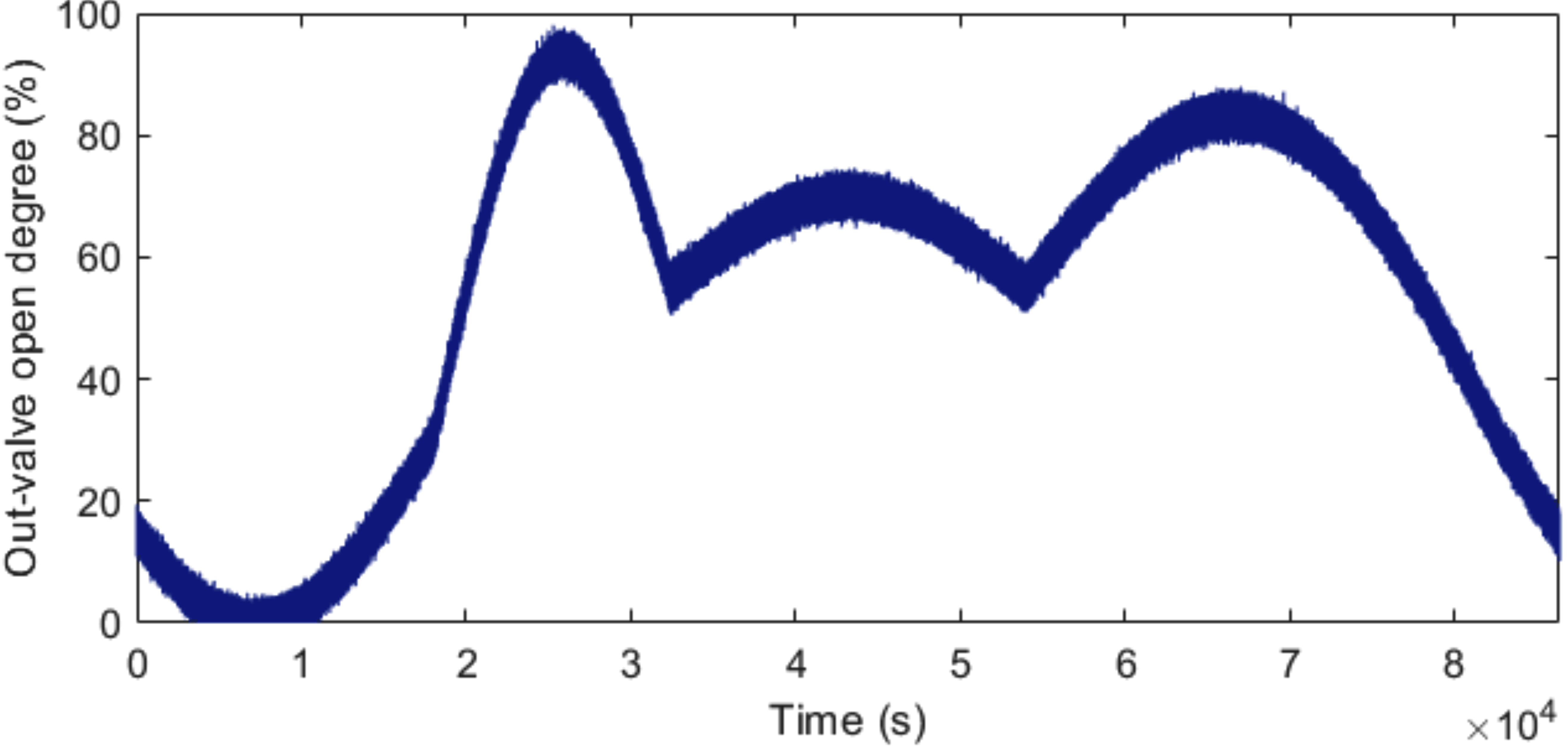
Figure 7. Daily customer demand ($24$ hours)

The results in Table 5 show that the $C^{3}$ system and LoRaWAN++ can both maintain systems stability through keeping small overshoots. The events per minute for the $C^{3}$ system are half of those for LoRaWAN++ with $\sigma=0.3$ and are within the maximum load that the system can handle as described in Sec. 3.3. The $C^{3}$ system also has nearly twice the E2E PDR and 75% smaller E2E Delays compared to LoRaWAN++. The $C^{3}$ system’s E2E Delays are bounded by a maximum of 2.1 seconds. The E2E Delays for LoRaWAN++ are 8 seconds on average. The increase in E2E Delays and reduction of E2E PDR shows that a change in customer demand causes the LoRaWAN++ network load to approach its capacity and struggles to meet the co-design criteria C₂.

Table 5. Evaluation of the $C^{3}$ system for dynamic customer demand compared to idealistic wired control and LoRaWAN++ for control.

$C^{3}$ system	Events/minute	OvSh (%)	E2E PDR (%)	E2E Delays (s)
$h=4.5$s, $\sigma=0.1$	50.33	6.67	87.3	2.043
$h=4.5$s, $\sigma=0.3$	34.80	6.0039	88.88	1.825
Wired Control	Events/minute	OvSh (%)	E2E PDR (%)	E2E Delays (s)
$h=4.5$s	133.33	3.44	100	0
LoRaWAN++	Events/minute	OvSh (%)	E2E PDR (%)	E2E Delays (s)
$h=4.5$s, $\sigma=0.1$	69.85	6.463	46.13	8.546
$h=4.5$s, $\sigma=0.3$	58.71	7.868	55.2	8.268

Study 3: Fault Detection. An important requirement of a water distribution network system is fault detection, when pipes burst due to sub-zero temperatures. A pipe burst causes water leakage which is another source of demand on a system. In this scenario, we assume that the sensors are able to take readings from the pipes (flow or vibrations) and determine if there is a leakage.

The leak detection mechanism identifies a fault and communicates this to enable leakage mitigation. The controller closes the valves that provide water to the affected area, re-routing water and preventing waste. The authors of (Kartakis et al., 2016) provide an example of this with leakage localisation to $50$cm (Yu and McCann, 2015).

The system state response is depicted in Fig. 8 and has three phases: no-fault (P1), fault (P2) and recovery from fault (P3). We give results in Table 6. The overshoots are comparable and stability is maintained. The E2E PDR of the $C^{3}$ system is almost twice that of LoRaWAN++. The E2E Delays are less than 2.1 seconds. The number of events/minute are within the maximum network load of $136$ packets/minute and achieve high reliability.

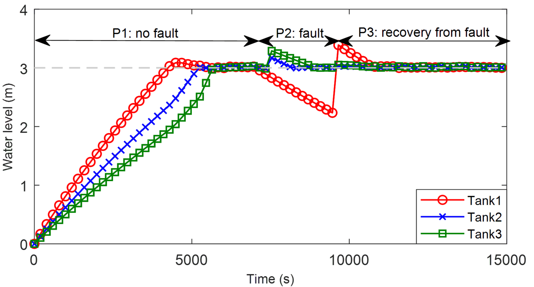
Figure 8. System response to a fault in the tank $1$.

Table 6. The evaluation of the $C^{3}$ system for constant customer demand with fault in comparison with an idealistic wired control and LoRaWAN for control.

$C^{3}$ system	Events/minute	OvSh (%)	E2E PDR (%)	E2E Delays (s)
$h=4.5$s, $\sigma=0.1$	P1: 25.03	3.3087	91.35	2.029
	P2: 64.34	16.059
	P3: 58.98	35.663
$h=4.5$s, $\sigma=0.3$	P1: 14.07	4.4741	92.25	1.789
	P2: 41.87	6.3206
	P3: 39.18	13.260
Wired Control	Events/minute	OvSh (%)	E2E PDR (%)	E2E Delays (s)
$h=4.5$s	P1: 133.33	2.75	100	0
	P2: 122.65	5.9129
	P3: 133.32	10.23
LoRaWAN++	Events/minute	OvSh (%)	E2E PDR (%)	E2E Delays (s)
$h=4.5$s, $\sigma=0.1$	P1: 25.52	3.0926	50.35	8.465
	P2: 69.35	19.29
	P3: 72.50	17.62
$h=4.5$s, $\sigma=0.3$	P1: 15.08	4.1367	60.94	6.875
	P2: 38.25	7.4541
	P3: 38.34	4.2372
		P1 - no fault, P2 - fault, P3 - recovery from fault

The results in Table 5 show that LoRaWAN++ maintains system stability not by design but by accident. The E2E Delays of LoRaWAN++ are four times higher than those of the $C^{3}$ system. Analysis of the simulation traces reveal that LoRaWAN++ succeeds in sending uplink messages to the gateway, but gateway acknowledgements are lost due to duty-cycle, $DC$, constraints. The loss of acknowledgement messages causes a resend. The gateway forwards the received, unacknowledged, sensor value to the controller, regardless of whether the sensor receives an acknowledgement. The sensor value leads to an actuation update and a stable system. The traces show that LoRaWAN++ is incapable of meeting our co-design constraint C₂, of maintaining the network load within its capacity. The freshness property of the sent data also enables LoRaWAN++ to maintain system stability. When a node fails to receive an acknowledgement before an event causes the sampling of new data, the new data replaces the old in the re-transmitted packet. In the case of lost acks and re-transmissions, the controller always receives the newest data and maintains system stability. Our next study investigates whether the stability by accident of LoRaWAN++ scales to a large-scale system.
Study 4: Large-Scale System. In this co-simulation, we model a larger system with 10 DMAs consisting of 32 sensor and actuator nodes. We use constant customer demand, two sampling intervals, $h$, of $1$ and $4.5$ seconds, and we run the experiment for $10000$ seconds.

The results in Table 7 show that at this scale LoRaWAN++ is unable to maintain overshoots within the system boundaries and the controller is unable to maintain system stability. The $C^{3}$ system can maintain stability while achieving overshoots of 22% and a good performance in terms of E2E PDR and E2E Delays, which is consistent with the three previous studies.

Table 7. The evaluation the $C^{3}$ system for 10 DMAs (32 nodes) in comparison with LoRaWAN++ for control.

$C^{3}$ System	Events/minute	OvSh (%)	E2E PDR (%)	E2E Delays (s)
$h=1$s	253.93	32.44	63.35	3.36
$h=4.5$s	115.20	22.39	88.16	4.01
LoRaWAN++	Events/minute	OvSh (%)	E2E PDR (%)	E2E Delays (s)
$h=1$s	238.77	46.80	26.9	11.28
$h=4.5$s	174.26	63.03	45.2	14.9

To conclude, our co-simulation results show that when the scale of the system increases by a factor of 3, LoRaWAN++ is no longer able to keep the network load within the capacity of the network and maintain system stability. This confirms our statement in Sec. 3.4 that the ALOHA channel access scheme is unable to provide the communication requirements for control, and our motivation for the creation of the two co-design constraints for our $C^{3}$ approach and the Ctrl-MAC.

5.2. Real World Evaluation

This section looks at the performance of the $C^{3}$ system designed using our $C^{3}$ approach on real hardware. For completeness, we apply a hybrid approach that combines a physical LoRa communication network with a simulated model of a water supply network to create a hardware-in-the-loop experiment and a hardware-in-the-park experiment. This stage of the evaluation validates the findings from the simulations showing that Ctrl-MAC and the controller can function correctly when tested with the uncertainty of real-world radio behaviours.

Real-world water distribution networks have mixed environments where they are deployed indoors and outdoors. We carry out hardware-in-the-loop experiment to characterise the behaviour of the $C^{3}$ system in an indoor environment. In this experiment, there is no line of sight between nodes. They are separated by plaster, brick and metal walls at distances on the order of tens of meters. We divide ten sensor nodes into three groups, each representing a single DMA.

The hardware-in-the-park experiment is done in a $2\times 2{\text{km}^{2}}$ urban park. This experiment has buildings, trees and large ornamental structures blocking line-of-sight. The distances of the hardware-in-the-park experiments are in the order of hundreds of meters. In this experiment, 8 sensor nodes are divided up into two DMAs.

Ctrl-MAC is implemented on all sensor nodes. Each node consists of an Adafruit Feather M0 RFM95 LoRa board mounted on a Raspberry Pi Model 3. Both the Pi and the Feather are powered by large capacity batteries. The gateway for the LoRa network is a MultiConnect Conduit Gateway connected to a desktop via Ethernet. The gateway uses an 868MHz +3dbi whip antenna. We altered the packet forwarder software to provide a timestamp to upper layers of the gateway stack running on the desktop. The desktop runs Gateway-Bridge to receive communication from the gateway. The Gateway-Bridge then sends the messages to LoRa Server, for decryption. Following this, the LoRa Server sends the decrypted messages to an App Server. The entire software stack on the desktop is provided by ChripStack.
Study 1: Hardware-in-the-Loop. Experimental setup is given in Fig. 9 (left).

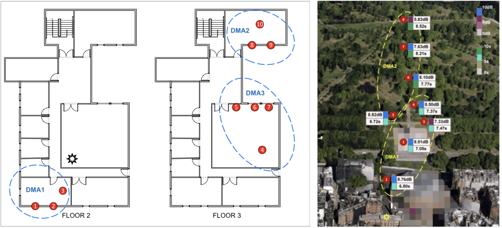
Figure 9. (left) Hardware-in-the-Loop experimental setup, (right) Hardware-in-the-Park experimental setup with up-stream delay and SNR values as seen at the gateway (the gateway is marked by the star, individual sensor nodes locations by red circles).

We provide the sensor nodes with a constant demand workload from the physical system simulator as seen in the first co-simulation experiment. We record the E2E Delays to measure the ability of our system to satisfy $\tau_{d}$, and the overshoot to assess the ability of our approach to maintain system stability.

The results are presented in Table. 8. There is a constant offset difference between the co-simulation delays and the experiment delays. These are due to issues with the hardware implementation at the gateway and unidentified latencies in the LoRa server software stack as the current LoRaWAN stack is not designed for real-time operation. In spite of these added delays, the overshoots are still small and show that our $C^{3}$ approach can maintain system stability.

Table 8. Round Trip Times and Overshoot for Hardware-in-the-loop experiment.

Node ID	1	2	3	4	5	6	7	8	9	10
Round Trip Time (s)	4.8	4.7	4	4.85	5.78	5.67	4.32	5.21	3.97	5.7
Overshoot (%)	4.98	17.25	3.8	8.4	12.36	7.22	9.64	4.98	16.6	13.3

Study 2: Hardware-in-the-Park. The experimental setup is shown in Fig. 9 (right). We chose this setup to provide realistic radio noise and effects such as the signal strength drop caused by distance and random interference. These real-world disturbances are very difficult to categorise and model in simulation. It is important to note that the small +3dbi whip antenna that we used on the gateway limited the range that we could achieve. The placement of the gateway, in the window of a building with line of site to the park, was also far from ideal and reduced our overall range.

This experiment differs from the previous hardware-in-the-loop because it does not use input directly from the simulator. Instead, this experiment uses event traces recorded from the simulator on every sensor node. We measured the Round Trip Times (RTTs) and signal to noise ratio (SNR) at the gateway for each node in this experiment. RTTs are defined as the difference between when a packet was acknowledged and when it was generated.

The results are depicted in Fig. 9 (right). It can be seen that the average delay between two successful events is small, very similar to the previous hardware-in-the-loop experiments. The signal to noise ratios show that there is a correlation between distance, SNR and delays. This is an indication of higher packet loss and retransmissions. We see that, even in the presence of an unstable radio link environment, the $C^{3}$ system keeps the delays bounded. It is clear that the bounded delay times that we observed in both of our real world experiments validate the co-simulation results and that our $C^{3}$ approach is useful to design control and communication protocols that can maintain the stability of a WA-CPS.
Experimental Observations. During our experimental evaluation with real sensor nodes, we encountered some strange packet loss behaviour that was the result of collisions and the capture effect (Voigt et al., 2017). The capture effect occurs when two packets arrive at the same time and there is a collision. One of the two packets is successfully decoded if the resulting RSSI of the received packet is higher than the receiver noise floor after the RSSI of the lost packet has been subtracted from it. The result is that the SNR value of the decoded packet reduces. For experiments involving hardware, we used low SNR thresholds to indicate the occurrence of collisions when the gateway had detected none. The gateway would then communicate to the node that did not successfully send its packet that it needed to restart the data sending process. We calculate SNRs at various positions and derived a threshold SNR value of 7dB in the laboratory, and between 6dB and 8dB for sensors in the outdoor experiment.

The capture effect can be seen in Fig. 10 that shows two nodes that transmit at the same time. The SNR for both nodes is between 9dB and 10dB for when there are no collisions. During a collision with the capture effect, we see that the SNR of the received packets is between 5dB and almost 0dB. We adapted Ctrl-MAC to use SNR threshold to detect collisions, which solved the problem.

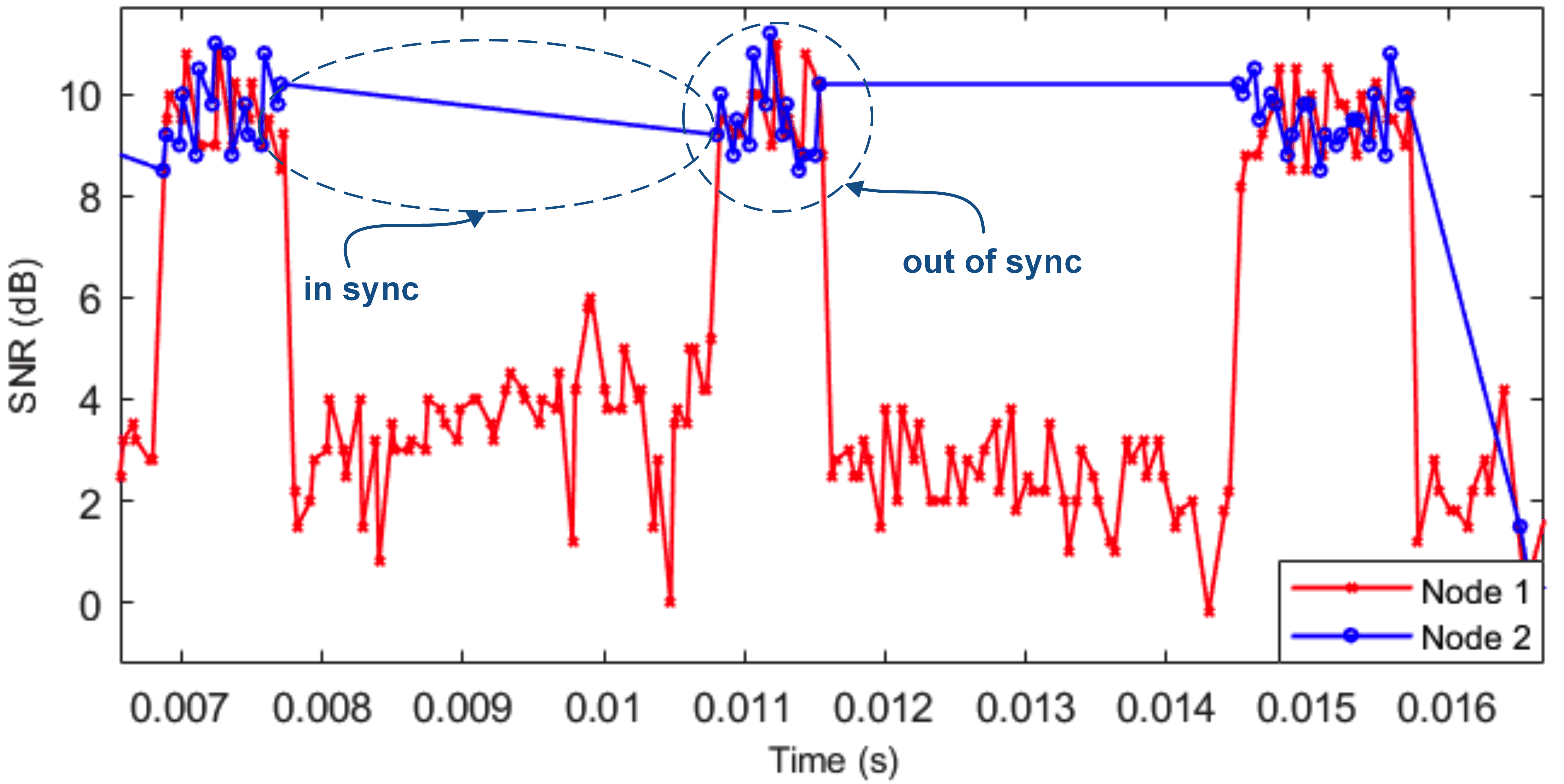
Figure 10. Capture effect phenomenon.

5.3. Evaluation Conclusion

The results of our evaluation clearly show that the use of our $C^{3}$ approach enabled the co-design of Ctrl-MAC and a controller that can maintain the E2E communication delay bounds required to keep a WA-CPS physical system stable. The results in Table 6 show that LoRaWAN++ and the $C^{3}$ system can maintain system stability on a 3 DMA system, although LoRaWAN++ has an E2E PDR of 50% to 60% compared to 91-100% for our $C^{3}$ system. At this scale, LoRaWAN++ enables stability for small scale control systems by accident as described in Sec. 5.1. As can be seen from Study 4, this situation does not scale well, and LoRaWAN++ fails when the system scale increases. In Table 7, we see that with 10 DMAs and 32 sensors LoRaWAN++ allows the overshoots to get as large as 63%. The $C^{3}$ system keeps the overshoots down to 22% for the same parameters. The E2E PDR falls to 26% for LoRaWAN++, while the $C^{3}$ system has an E2E PDR of 63% at a sample interval of 1 second. Thus, the results of the evaluation show benefits of the $C^{3}$ system over LoRaWAN++.

6. Related Work

The contribution of this paper is in the combination of control and wireless computer communication. There is a large body of literature focusing on wireless network control systems both by co-designing the communication and control and considering them individually (Park et al., 2018). We limit our review of the literature to event-triggered control and off-the-self wireless communication systems that have been used in such control systems. Similar approaches to the combination of control and communication are (Tubaishat et al., 2007; Suryadevara et al., 2015; Pellegrino et al., 2016; Liu and Goldsmith, 2004; Petersen and Carlsen, 2011; Eisen et al., 2019; Fadel et al., 2015; Schindler et al., 2017) but do not focus on event-triggered control.

The most relevant work from the event-triggered control literature comes from (Mazo and Tabuada, 2011; Mazo Jr and Fu, 2015; Jin et al., 2019; Wang and Lemmon, 2011). In (Wang and Lemmon, 2011), authors examine the bounds required to achieve event-triggered control. They use canonical control systems that do not reflect the complexity of real-world practical physical systems. Their work only addresses short-range communications (such as Zigbee) with high data rates and the inability to scale to multi-kilometres. In (Mazo and Tabuada, 2011), the complexity of disturbances was ignored, and all sensors communicate local measurements synchronously. Both of these assumptions do not apply to large-scale physical systems. In (Wang and Lemmon, 2011), the event trigger mechanism and controller are decentralised, making local computation complex (not suitable for low-powered sensor devices). In (Jin et al., 2019) the authors propose real-time scheduling for event-triggered and time-triggered flows using 802.15.4 compliant radios. In (Mazo Jr and Fu, 2015) the authors propose a decentralised event-triggered control with a TDMA protocol and reserved slots which will not scale to a large number of low-power nodes.

The closest experimental works to ours from the event-triggered control literature includes (Araújo et al., 2014; Kartakis et al., 2018; Mager et al., 2019). In (Araújo et al., 2014), the system dynamics are entirely different from our own. The system has double tanks, a small area, uses Zigbee, and requires fast control of $20$ seconds to reach equilibrium. Our system has 10 tanks, covers a considerably larger area, uses LPWA, and is slow-loop requiring $4500$ seconds to reach equilibrium (see Fig. 6). The use of TDMA in (Araújo et al., 2014) negatively impacts scale because nodes have to await their turn. Ctrl-MAC uses request slots to allow multiple nodes to request to send data immediately. The work in (Kartakis et al., 2018) considers centralised and decentralised event-triggered control of water systems. It also assumes LAN scale system on a small-scale emulator and not a distributed multi-subsystem. Exciting work by (Mager et al., 2019) derived communication schemes with guaranteed closed-loop stability for linear dynamic systems over low-power multi-hop networks. Their end-to-end design assumes a bespoke communication system based on constructive interference for control message flooding. The range of their solution is also limited to LAN scaled areas and not the wide-area multi-sub-system distributed control described in our paper.

7. Limitations

While this paper aims to demonstrate that LPWA communication technologies can indeed support WA-CPS, there are some limitations to our exposition that we reserve for further research. Firstly, we do not explicitly discuss energy usage or saving. It is implicit in the way that we save large volumes of communication messages. However, we accept that actuation is relatively power-hungry (e.g. a pump) we either assume it is wired or uses energy harvesting and we have modelled the actuators as listening to the channel at all times, therefore we do not explicitly present energy costs of these in the results. Future work will look into minimising the listening time of the actuators to save energy. All other energy savings come from standard sensor communications approaches inherent in the lightweight LPWA protocol. We scale our work to 150 nodes per base-station as per general LoRa recommendations. In real implementations of LoRa scale is achieved through the deployment of more gateways. However, this would expose different scheduling problems to manage feedback messages between many gateways to a given node; therefore, further work on slot allocation to cope with, or ensure, non-overlapping communications is required. Robust analysis of a communications protocol in a control scenario dictates its analysis in terms of a canonical physical system, in our case, the water distribution network. This system was chosen as it represents the dynamics of many multi-kilometre pipeline systems, further work on other applications will demonstrate generality further.

8. Conclusion

In this paper, we present Ctrl-MAC, a novel LPWA MAC protocol that balances the control requirements of WA-CPS with the communication limitations imposed by LPWA communication technologies. Our protocol is a product of a Control Communication Co-design ($C^{3}$) approach for WA-CPSs. The $C^{3}$ approach specifies a set of control and communication parameters and the constraints that couple them to create a controller and communication protocol that can maintain stability for a WA-CPS. Our evaluation shows that Ctrl-MAC and its controller, referred to as the $C^{3}$ system, can maintain system stability under real-world conditions. The results of our co-simulation evaluation show that neither LoRaWAN nor LoRaWAN++ can provide data reception guarantees to the sensors or the control system. Ctrl-MAC has up to $50$% better average packet delivery ratio and $80$% less average end-to-end delays when compared to LoRaWAN++. The combination of guarantees and low latencies makes Ctrl-MAC the only LPWA system suitable for the long range communication and control of WA-CPSs.

The evaluation criterion used in this paper aims to be acceptable to both the computer systems community (via reasoned algorithms, extensive scaled evaluations and real-world testing) and the control community (via formal reasoning of a physical water distribution control system). Our evaluation shows that Ctrl-MAC in the $C^{3}$ system succeeds in maintaining stability based on the criterion that we establish for WA-CPS. This work is the first to demonstrate that LPWA communications, specifically (LoRa), can conclusively support a large class of control systems, previously considered beyond its scope. Our future work will continue to explore various applications of Ctrl-MAC in the wild.

Appendix A Appendix

A.1. Proof of Corollary 4.1

Proof.

The basic idea of the proof is inspired by the proofs of Theorem III.4 in (Borgers et al., 2018) and Theorem III.2 and Corollary III.3 in (Heemels et al., 2013). The proof consists of three main steps which are presented next.

In the first step, we consider the following Lyapunov function:

(9) $$V(\xi,\tau)=\left\{\begin{aligned} &\xi^{\mathrm{T}}P_{1}(\tau)\xi,\,\tau\in[0,\tau_{d}]\\ &\xi^{\mathrm{T}}P_{0}(\tau)\xi,\,\tau\in[\tau_{d},h]\\ \end{aligned}\right.$$

where

(10) $$\frac{\mathrm{d}}{\mathrm{d}\tau}P_{i}=-\bar{A}^{\mathrm{T}}P_{i}-P_{i}\bar{A}-2\rho P_{i}$$

with $i\in\{1,0\}$. The matrices $P_{0h}$ and $P_{1d}$ are defined in Corollary 4.1 as $P_{0}(h)=P_{0h}$ and $P_{1}(\tau_{d})=P_{1d}$. Additionally, we define $P_{10}:=P_{1}(0)$, and $P_{0d}:=P_{0}(\tau_{d})$.

We also consider two scalars $c_{1}$ and $c_{2}$ that satisfy $0<c_{1}\leq c_{2}$ and are given as:

$$c_{1} :=\min\{\min_{\tau\in[0,\tau_{d}]}\lambda_{\min}(P_{1}(\tau)),\min_{\tau\in[0,h]}\lambda_{\min}(P_{0}(\tau))\}$$

$$c_{2} :=\max\{\max_{\tau\in[0,\tau_{d}]}\lambda_{\max}(P_{1}(\tau)),\max_{\tau\in[0,h]}\lambda_{\max}(P_{0}(\tau))\}$$

where $\lambda_{\min}(P_{i})$ and $\lambda_{\max}(P_{i})$ are the minimum and maximum eigenvalues of matrix $P_{i}$, respectively. According to (Borgers et al., 2018) and (Heemels et al., 2013), it can be show that the function $V$ satisfies the following inequalities:

$$c_{1}|\xi|^{2}\leq V(\xi,\tau)\leq c_{2}|\xi|^{2}.$$

In the second step, we analyse $V$ during the flows and jumps of the system. Using Eq. 9 and Eq. 10, and derivating $V$ along $\tau$ ($V$: $\tau\in[0,\tau_{d}]$ and $\tau\in[\tau_{d},h]$) we get:

$$\frac{\mathrm{d}}{\mathrm{d}t}V(\xi,\tau)=-2\rho V(\xi,\tau).$$

In the third step, we need to show that $V$ does not increase during jumps. According to (Heemels et al., 2013), it holds that

(11) $$P_{10} =e^{2\rho\tau_{d}}e^{\bar{A}^{\mathrm{T}}\tau_{d}}P_{1d}e^{\bar{A}\tau_{d}}$$

$$P_{0d} =e^{2\rho(h-\tau_{d})}e^{\bar{A}^{\mathrm{T}}(h-\tau_{d})}P_{0h}e^{\bar{A}(h-\tau_{d})}.$$

By applying Schur complement and S-procedure, it follows from Eq. 8 that:

$$\xi^{+\mathrm{T}}P_{10}\xi^{+}=\xi^{\mathrm{T}}\acute{J}_{\mathcal{J}}^{\mathrm{T}}P_{10}\acute{J}_{\mathcal{J}}\xi\leq\xi^{\mathrm{T}}P_{0h}\xi$$

$$\xi^{+\mathrm{T}}P_{0d}\xi^{+}=\xi^{\mathrm{T}}\tilde{J}_{\mathcal{J}}^{\mathrm{T}}P_{0d}\tilde{J}_{\mathcal{J}}\xi\leq\xi^{\mathrm{T}}P_{1d}\xi.$$

The results of this proof guarantee that $V$ is a proper Lyapunov function and the system is GES with convergence rate $\rho$ which concludes the proof. ∎

References

- (1)
- Adelantado et al. (2017) Ferran Adelantado, Xavier Vilajosana, Pere Tuset-Peiro, Borja Martinez, Joan Melia-Segui, and Thomas Watteyne. 2017. Understanding the limits of LoRaWAN. IEEE Commun. Magazine 55, 9 (2017), 34–40.
- Araújo et al. (2014) José Araújo, Manuel Mazo, Adolfo Anta, Paulo Tabuada, and Karl H Johansson. 2014. System architectures, protocols and algorithms for aperiodic wireless control systems. IEEE Trans. on Industrial Informatics 10, 1 (2014), 175–184.
- Belimo (2019) Belimo. 2019. NRQ24A-SR Datasheet. https://www.belimo.ch/pdf/e/NRQ24A-SR_datasheet_en-gb.pdf. [Online; accessed 23-June-2019].
- Borgers et al. (2018) Dominicus Paulus Borgers, Victor Sebastiaan Dolk, and WPMH Heemels. 2018. Riccati-based design of event-triggered controllers for linear systems with delays. IEEE Trans. on Automatic Control 63, 1 (2018), 174–188.
- Chandrasekaran (2006) Balakrishnan Chandrasekaran. 2006. Survey of Network Traffic Models. https://www.cse.wustl.edu/~jain/cse567-06/ftp/traffic_models3.pdf. [Online; accessed 03-June-2019].
- Committee (2018) Lora Alliance Technical Committee. 2018. LoRaWAN 1.1 Specification. https://lora-alliance.org/sites/default/files/2018-07/lorawan1.0.3.pdf. [Online; accessed 03-June-2019].
- Dicken et al. (2012) James Dicken, Paul D Mitcheson, Ivan Stoianov, and Eric M Yeatman. 2012. Power-extraction circuits for piezoelectric energy harvesters in miniature and low-power applications. IEEE Trans. on Power Electronics 27, 11 (2012), 4514–4529.
- Eisen et al. (2019) Mark Eisen, Mohammad M. Rashid, Konstantinos Gatsis, Dave Cavalcanti, Nageen Himayat, and Alejandro Ribeiro. 2019. Control Aware Radio Resource Allocation in Low Latency Wireless Control Systems. IEEE Internet of Things Journal 6, 5 (2019), 7878–7890.
- Fadel et al. (2015) Etimad Fadel, Vehbi C Gungor, Laila Nassef, Nadine Akkari, MG Abbas Malik, Suleiman Almasri, and Ian F Akyildiz. 2015. A survey on wireless sensor networks for smart grid. Computer Commun. 71 (2015), 22–33.
- Gurung et al. (2015) Thulo Ram Gurung, Rodney A Stewart, Cara D Beal, and Ashok K Sharma. 2015. Smart meter enabled water end-use demand data: platform for the enhanced infrastructure planning of contemporary urban water supply networks. J. of Cleaner Production 87 (2015), 642–654.
- Heemels et al. (2013) WPM Heemels Heemels, MCF Donkers, and Andrew R Teel. 2013. Periodic event-triggered control for linear systems. IEEE Trans. on Autom. Control 58, 4 (2013), 847–861.
- Jin et al. (2019) X. Jin, A. Saifullah, C. Lu, and P. Zeng. 2019. Real-Time Scheduling for Event-Triggered and Time-Triggered Flows in Industrial Wireless Sensor-Actuator Networks. In IEEE INFOCOM 2019 - IEEE Conference on Computer Communications. 1684–1692.
- Kartakis et al. (2018) S. Kartakis, A. Fu, M. Mazo, and J. A. McCann. 2018. Communication Schemes for Centralized and Decentralized Event-Triggered Control Systems. IEEE Transactions on Control Systems Technology 26, 6 (2018), 2035–2048.
- Kartakis et al. (2016) Sokratis Kartakis, Weiren Yu, Reza Akhavan, and Julie A McCann. 2016. Adaptive edge analytics for distributed networked control of water systems. In 2016 IEEE First Int. Conf. on Internet-of-Things Design and Impl. IEEE, 72–82.
- Liu and Goldsmith (2004) Xiangheng Liu and Andrea Goldsmith. 2004. Wireless network design for distributed control. Proceedings of the IEEE Conference on Decision and Control 3 (2004), 2823–2829.
- Lu et al. (2016) Chenyang Lu, Abusayeed Saifullah, Bo Li, Mo Sha, Humberto Gonzalez, Dolvara Gunatilaka, Chengjie Wu, Lanshun Nie, and Yixin Chen. 2016. Real-time wireless sensor-actuator networks for industrial cyber-physical systems. Proc. of the IEEE 104, 5 (2016), 1013–1024.
- Mager et al. (2019) Fabian Mager, Dominik Baumann, Romain Jacob, Lothar Thiele, Sebastian Trimpe, and Marco Zimmerling. 2019. Feedback Control Goes Wireless: Guaranteed Stability over Low-power Multi-hop Networks. In Proc. of the 10th ACM/IEEE Int. Conf. on Cyber-Physical Sys. (ICCPS ’19). ACM, New York, NY, USA, 97–108.
- Mazo and Tabuada (2011) Manuel Mazo and Paulo Tabuada. 2011. Decentralized event-triggered control over wireless sensor/actuator networks. IEEE Trans. on Automatic Control 56, 10 (2011), 2456–2461.
- Mazo Jr and Fu (2015) Manuel Mazo Jr and Anqi Fu. 2015. Decentralized event-triggered controller implementations. Event-Based Control and Signal Processing (2015), 121.
- Moreau (2011) Alain Moreau. 2011. Control strategy for domestic water heaters during peak periods and its impact on the demand for electricity. Energy Procedia 12 (2011), 1074–1082.
- Park et al. (2018) Pangun Park, Sinem Coleri Ergen, Carlo Fischione, Chenyang Lu, and Karl H. Johansson. 2018. Wireless Network Design for Control Systems: A Survey. IEEE Commun. Surveys Tuts. 20, 2 (2018), 978–1013.
- Pellegrino et al. (2016) Anna Pellegrino, Valerio RM Lo Verso, Laura Blaso, Andrea Acquaviva, Edoardo Patti, and Anna Osello. 2016. Lighting control and monitoring for energy efficiency: a case study focused on the interoperability of building management systems. IEEE Trans. on Industry Applications 52, 3 (2016), 2627–2637.
- Petersen and Carlsen (2011) Stig Petersen and Simon Carlsen. 2011. WirelessHART versus ISA100. 11a: The format war hits the factory floor. IEEE Industrial Electronics Magazine 5, 4 (2011), 23–34.
- Pop et al. (2018) Alexandru-Ioan Ioan Pop, Usman Raza, Parag Kulkarni, and Mahesh Sooriyabandara. 2018. Does Bidirectional Traffic Do More Harm Than Good in LoRaWAN Based LPWA Networks? 2017 IEEE Global Commun. Conf. (2018), 1–6.
- Raza et al. (2017) Usman Raza, Parag Kulkarni, and Mahesh Sooriyabandara. 2017. Low power wide area networks: An overview. IEEE Commun. Surveys Tuts. 19, 2 (2017), 855–873.
- Schindler et al. (2017) Craig B Schindler, Thomas Watteyne, Xavier Vilajosana, and Kristofer SJ Pister. 2017. Implementation and characterization of a multi-hop 6TiSCH network for experimental feedback control of an inverted pendulum. In Modeling and Optimization in Mobile, Ad Hoc, and Wireless Networks (WiOpt), 2017 15th Int. Symp. on. IEEE, 1–8.
- Song et al. (2008) Jianping Song, Song Han, Al Mok, Deji Chen, Mike Lucas, Mark Nixon, and Wally Pratt. 2008. WirelessHART: Applying wireless technology in real-time industrial process control. In IEEE Real-Time and Embedded Tech. and Appl. Symp.
- Suryadevara et al. (2015) Nagender Kumar Suryadevara, Subhas Chandra Mukhopadhyay, Sean Dieter Tebje Kelly, and Satinder Pal Singh Gill. 2015. WSN-based smart sensors and actuator for power management in intelligent buildings. IEEE/ASME Trans. on Mechatronics 20, 2 (2015), 564–571.
- Tomić et al. (2018) Ivana Tomić, Laksh Bhatia, Michael J Breza, and Julie A McCann. 2018. The Limits of LoRaWAN in Event-Triggered Wireless Networked Control Systems. 2018 UKACC 12th Int. Conf. on Control (CONTROL) (2018), 101–106.
- Tubaishat et al. (2007) Malik Tubaishat, Yi Shang, and Hongchi Shi. 2007. Adaptive traffic light control with wireless sensor networks. In Consumer Commun. and Networking Conf., 2007. CCNC 2007. 4th IEEE. IEEE, 187–191.
- Vilajosana et al. (2019) Xavier Vilajosana, Thomas Watteyne, Mališa Vučinić, Tengfei Chang, and Kristofer S. J. Pister. 2019. 6TiSCH: Industrial Performance for IPv6 Internet-of-Things Networks. Proc. of the IEEE (2019), 1–13.
- Voigt et al. (2017) Thiemo Voigt, Martin Bor, Utz Roedig, and Juan Alonso. 2017. Mitigating Inter-network Interference in LoRa Networks. In Proc. of the 2017 Int. Conf. on Embedded Wireless Sys. and Netw. (EWSN). USA, 323–328.
- Wang and Lemmon (2011) Xiaofeng Wang and Michael D Lemmon. 2011. Event-triggering in distributed networked control systems. IEEE Trans. on Automatic Control 56, 3 (2011), 586.
- Yu and McCann (2015) Weiren Yu and Julie A. McCann. 2015. Effectively Positioning Water Loss Event in Smart Water Networks. The 2nd International Electronic Conference on Sensors and Applications (IECSA) (2015), 1–10.