Automated Reasoning in Temporal DL-Lite

Abstract

This paper investigates the feasibility of automated reasoning over temporal DL-Lite (TDL-Lite) knowledge bases (KBs). We test the usage of off-the-shelf LTL reasoners to check satisfiability of TDL-Lite KBs. In particular, we test the robustness and the scalability of reasoners when dealing with TDL-Lite TBoxes paired with a temporal ABox. We conduct various experiments to analyse the performance of different reasoners by randomly generating TDL-Lite KBs and then measuring the running time and the size of the translations. Furthermore, in an effort to make the usage of TDL-Lite KBs a reality, we present a fully fledged tool with a graphical interface to design them. Our interface is based on conceptual modelling principles and it is integrated with our translation tool and a temporal reasoner.

1 Introduction

Ontology languages are a central research topic in the Semantic Web community where OWL and its various fragments have been adopted as a W3C standard ontology language. While OWL allows to capture and reason over static ontologies, here we are interested in representing and reasoning over dynamic ontologies, i.e., ontologies able to capture the temporal behaviour of its main primitives (classes, object- and data-properties).

Reasoning over temporal ontologies has been studied in the literature on temporal representation languages (see [3, 23] for surveys on temporal extensions of description logics). The complexity of standard reasoning tasks, such as satisfiability and entailment, in $\smash{\mathcal{ALC}}$-based temporal DLs is known to be hard, ranging from ExpTime to undecidable [23, 7], while it becomes easier when extending DL-Lite-based DLs [6]. There is a growing interest in ontologies based on DL-Lite, which is the backbone of the W3C standard ontology language OWL 2 QL—the main formalism underpinning the OBDA paradigm [25, 1]. While temporal DL-Lites are not yet an OWL standard, they have nonetheless been studied as a formalism to represent and reason over dynamic ontologies, in particular when such ontologies have the shape of conceptual models [5, 6].

In this paper, we study the practical feasibility of reasoning over temporal DL-Lite (TDL-Lite) extensions. In particular, as TDL-Lite we consider here the $T_{FPX}DL$-$Lite^{\mathcal{N}}_{bool}$ logic, the most expressive of the tractable DL-Lite family combined with LTL  allowing for: full Boolean connectives in the construction of concepts, cardinalities and inverse constraints on roles, LTL-based temporal operators applied to concepts, distinction between global (i.e., time-invariant) and local roles. Ontologies in TDL-Lite are expressed via concept inclusion axioms, so called TBox, intended to express the constraints of a given application domain via axioms that hold at each point in time (i.e., a TBox expresses a global knowledge), paired with temporal assertions (i.e., a so called temporal ABox) expressing timestamped factual knowledge. The complexity of reasoning over TDL-Lite KBs, i.e., a set of TBox and ABox axioms, is known to be PSpace-complete [6].

The main purpose here is to collect experimental evidences on the feasibility of automated reasoning on TDL-Lite KBs by leveraging on existing off-the-shelf LTL solvers. The key idea is to map such KBs into equisatisfiable LTL formulas by applying the mapping described by Artale et al. (2014) [6]. Since TDL-Lite admits both past and future operators interpreted over $\mathbb{Z}$ while LTL reasoners deals just with $\mathbb{N}$, in our study, we also consider the simpler logic $\textsl{T}^{\mathbb{N}}\textsl{DL-Lite}$ that is able to express just future temporal formulas interpreted over $\mathbb{N}$. Our main contributions are:

1. the development of a non-trivial extension of the tool crowd [9] to draw temporal conceptual schemas, featuring an option to populate the schema with timestamped instances, which can be automatically mapped into TDL-Lite KBs;

2. the development of a linear equisatisfiable translation of TDL-Lite KBs into LTL formulas, with formal proofs for the strategy that removes past operators over the integers;

3. an experimental analysis measuring the runtime, and the size of the translation based on randomly generated TDL-Lite KBs, and an experimental analysis of toy scenarios exploiting the modelling capabilities of the language. We compare the performance of different LTL solvers on the various test cases we consider. For the randomly generated ontologies, we present benchmarks for the following cases: $(i)$ TDL-Lite TBoxes; and $(ii)$ $\textsl{T}^{\mathbb{N}}\textsl{DL-Lite}$  TBoxes. As for the toy scenario, we evaluate the perfomances with ABoxes of increasing sizes.

In the following, we present our running examples to provide an intuitive overview on the expressive power of TDL-Lite. These examples are also part of our experimental tests.

Example 1

Let’s consider first the simple case of a person who might be minor or adult. This can be modelled by the following TDL-Lite TBox:

$$\mathcal{T}=\{{\sf Adult}\sqsubseteq{\sf Person},{\sf Minor}\sqsubseteq{\sf Person},{\sf Minor}\sqcap{\sf Adult}\sqsubseteq\bot,{\sf Adult}\sqsubseteq\Box_{F}{\sf Adult}\}$$

In words, $\mathcal{T}$ states that minors and adults are persons, but they are disjoint. Moreover, adult is persistent in the future—expressed by the temporal operator always in the future $\Box_{F}$. Now, assume one wants to check the consistency of the following ABox, reporting on the status of the person John at different timestamps, w.r.t. the TBox $\mathcal{T}$:

$$\mathcal{A}=\{{\sf Person}({\sf John},0),{\sf Minor}({\sf John},0),{\sf Adult}({\sf John},1),{\sf Minor}({\sf John},2),{\sf Adult}({\sf John},3)\}$$

According to the persistence of being adult together with the fact that adult is disjoint from minor, the ABox $\mathcal{A}$ is inconsistent w.r.t. $\mathcal{T}$. $\triangleleft$

In the following example we show another critical case of inconsistency due to the interaction between cardinalities and global roles, i.e., binary relations whose instances are time-invariant.

Example 2

Consider the following knowledge base, $\mathcal{K}=(\mathcal{T},\mathcal{A})$, where the TBox assumes that each person has a Name being a global functional role (role names are distinguished being either global or local in the signature of the logic, see next Section):

$$\mathcal{T} =\{{\sf Person}\sqsubseteq\geq 1\leavevmode\nobreak\ {\sf Name},{\sf Person}\sqsubseteq\lnot\geq 2\leavevmode\nobreak\ {\sf Name}\}$$

$$\mathcal{A} =\{{\sf Person}(p_{1},0),{\sf Name}(p_{1},{\sf\textit{Kennedy}},0),{\sf Name}(p_{1},{\sf\textit{Marc}},1)\}$$

In words, $\mathcal{T}$ states that each person has a single name which, in turns, is a global role. On the other hand, while at each point in time, $p_{1}$ has exactly one name, $p_{1}$ has different names at different points in time. Thus, $\mathcal{A}$ violates the fact that name is both functional and global, and $\mathcal{K}$ is then inconsistent. $\triangleleft$

This paper is organised as follows. Section 2 introduces the temporal DL TDL-Lite. Section 3 describes the equisatisfiable encoding from TDL-Lite to LTL. Section 4 describes the architecture of the tool we are proposing. Section 5 illustrates the experimental setting and reports on the performances obtained by using different solvers to reason over TDL-Lite KBs. We report our concluding remarks in Section 6.

2 Temporal Description Logic

We briefly introduce the syntax and the semantics of the temporal description logic TDL-Lite. In this paper by TDL-Lite we denote the logic $\smash{\textsl{T}_{F\!P\!X}\textsl{DL-Lite}_{\textit{bool}}^{\cal N}}$, the fragment of $\textsl{T}_{\mathbin{\mathcal{U}}\mathbin{\mathcal{S}}}\textsl{DL-Lite}_{\textit{bool}}^{\mathcal{N}}$, introduced in [6], that allows the past and future temporal operators $\Box,\Diamond,\ocircle$. We notice that while the complexity of $\textsl{T}_{\mathbin{\mathcal{U}}\mathbin{\mathcal{S}}}\textsl{DL-Lite}_{\textit{bool}}^{\mathcal{N}}$, which allows for both $\mathcal{U}$ and $\mathcal{S}$, is the same as $\smash{\textsl{T}_{F\!P\!X}\textsl{DL-Lite}_{\textit{bool}}^{\cal N}}$, $\mathcal{U}$ and $\mathcal{S}$ are barely used in conceptual modelling [6, 5]. We consider in this paper the non-strict semantics of the diamond and box operators (as usual, strictness can be expressed using the next operator, e.g., strict diamond in the future is ${\raisebox{1.07639pt}{\text{\scriptsize{$\bigcirc$}}}}_{\!\scriptscriptstyle F}\Diamond_{\!\scriptscriptstyle F}C$). Let ${\sf N_{C}},{\sf N_{I}}$ be countable sets of concept and individual names, respectively, and let $\textsf{N}_{\textsf{G}}$ and $\textsf{N}_{\textsf{L}}$ be countable and disjoint sets of global and local role names, respectively. The union $\textsf{N}_{\textsf{G}}\cup\textsf{N}_{\textsf{L}}$ is the set ${\sf N_{R}}$ of role names. TDL-Lite roles $R$, basic concepts $B$, and (temporal) concepts $C$ are given by the following grammar:

$$R ::=L\mid L^{-}\mid G\mid G^{-}, B ::=\bot\mid A\mid\,\geq qR,$$

$$C ::=B\mid\lnot C\mid C_{1}\sqcap C_{2}\mid\Diamond_{F}C\mid\Diamond_{P}C\mid\ocircle_{F}C\mid\ocircle_{P}C,$$

where $L\in\textsf{N}_{\textsf{L}}$, $G\in\textsf{N}_{\textsf{G}}$, $A\in{\sf N_{C}}$, and $q\in\mathbb{N},q>0$ (given in binary).

We use standard abbreviations for concepts: $\top:=\lnot\bot$, $(C_{1}\sqcup C_{2}):=\lnot(\lnot C_{1}\sqcap\lnot C_{2})$, $\exists R:=\geq 1R$, $\ocircle^{n+1}C:=\ocircle_{F}\ocircle_{F}^{n}C$, with $n\geq 0$ (we set $\ocircle^{0}C:=C$), $\ocircle^{n-1}C:=\ocircle_{P}\ocircle_{P}^{n}C$, with $n<0$, $\Box_{F}C:=\neg\Diamond_{F}\neg C$, $\Box_{P}C:=\neg\Diamond_{P}\neg C$, $\mathop{\ooalign{$\Box$\cr\kern 1.80832pt\raisebox{1.50696pt}{\scalebox{0.7}{$*$}}}\rule{0.0pt}{6.45831pt}\kern-3.01385pt}C=\Box_{\!\scriptscriptstyle F}\Box_{\!\scriptscriptstyle P}C$, and $\mathop{\ooalign{$\Diamond$\cr\kern 2.15277pt\raisebox{1.50696pt}{\scalebox{0.7}{$*$}}}\kern-3.87495pt}C=\Diamond_{\!\scriptscriptstyle F}\Diamond_{\!\scriptscriptstyle P}C$.

A TDL-Lite axiom is either a concept inclusion (CI) of the form $C_{1}\sqsubseteq C_{2}$, a concept assertion of the form $\ocircle^{n}A(a)$ or $\ocircle^{n}\neg A(a)$, or a role assertion of the form $\ocircle^{n}R(a,b)$ or $\ocircle^{n}\neg R(a,b)$, where $C_{1},C_{2}$ are TDL-Lite concepts, $A\in{\sf N_{C}}$, $R\in{\sf N_{R}}$, $a,b\in{\sf N_{I}}$, and $n\in\mathbb{Z}$. A TBox is a set of CIs and an ABox is a set of (concept and role) assertions. A TDL-Lite knowledge base, $\mathcal{K}$, is a pair $\mathcal{K}=(\mathcal{T},\mathcal{A})$, where $\mathcal{T}$ is a TBox and $\mathcal{A}$ is an ABox.

A TDL-Lite interpretation is a structure $\mathfrak{M}=(\Delta^{\mathfrak{M}},(\mathcal{I}_{n})_{n\in\mathbb{Z}})$, where each $\mathcal{I}_{n}$ is a classical DL interpretation with non-empty domain $\Delta^{\mathfrak{M}}$ (or simply $\Delta$). We have that $A^{\mathcal{I}_{n}}\subseteq\Delta^{\mathfrak{M}}$ and $S^{\mathcal{I}_{n}}\subseteq\Delta^{\mathfrak{M}}\times\Delta^{\mathfrak{M}}$, for all $A\in{\sf N_{C}}$ and $S\in{\sf N_{R}}$. In particular, for all $G\in\textsf{N}_{\textsf{G}}$ and $i,j\in\mathbb{Z}$, $G^{\mathcal{I}_{i}}=G^{\mathcal{I}_{j}}$ (denoted simply by $G^{\mathcal{I}}$). Moreover, $a^{\mathcal{I}_{i}}=a^{\mathcal{I}_{j}}\in\Delta^{\mathfrak{M}}$ for all $a\in{\sf N_{I}}$ and $i,j\in\mathbb{Z}$, i.e., constants are rigid designators (with fixed interpretation, denoted simply by $a^{\mathcal{I}}$). The interpretation of individuals further respects the unique name assumption UNA, i.e., $a^{\mathcal{I}}\neq b^{\mathcal{I}}$ if $a\neq b$. The stipulation that all time points share the same domain $\Delta^{\mathfrak{M}}$ is called the constant domain assumption (meaning that objects are not created nor destroyed over time). The interpretation of roles and concepts at instant $n\in\mathbb{Z}$ is defined as follows (where $S\in{\sf N_{R}}$):

$$(S^{-})^{\mathcal{I}_{n}}=\{(d^{\prime},d)\in\Delta^{\mathfrak{M}}\times\Delta^{\mathfrak{M}}\mid(d,d^{\prime})\in S^{\mathcal{I}_{n}}\},\qquad\bot^{\mathcal{I}_{n}}=\emptyset,$$

$$(\geq qR)^{\mathcal{I}_{n}}=\{d\in\Delta^{\mathfrak{M}}\mid\sharp\{d^{\prime}\in\Delta^{\mathfrak{M}}\mid(d,d^{\prime})\in R^{\mathcal{I}_{n}}\}\geq q\},$$

$$(\neg C)^{\mathcal{I}_{n}}=\Delta^{\mathfrak{M}}\setminus C^{\mathcal{I}_{n}},\qquad(C_{1}\sqcap C_{2})^{\mathcal{I}_{n}}=C_{1}^{\mathcal{I}_{n}}\cap C_{2}^{\mathcal{I}_{n}},$$

$$(\ocircle_{F}C)^{\mathcal{I}_{n}}=\{d\in\Delta^{\mathfrak{M}}\mid\ d\in C^{\mathcal{I}_{n+1}}\},\quad(\ocircle_{P}C)^{\mathcal{I}_{n}}=\{d\in\Delta^{\mathfrak{M}}\mid\ d\in C^{\mathcal{I}_{n-1}}\},$$

$$(\Diamond_{F}C)^{\mathcal{I}_{n}}=\{d\in\Delta^{\mathfrak{M}}\mid\exists m\in\mathbb{Z},m\geq n\colon d\in C^{\mathcal{I}_{m}}\},$$

$$(\Diamond_{P}C)^{\mathcal{I}_{n}}=\{d\in\Delta^{\mathfrak{M}}\mid\exists m\in\mathbb{Z},m\leq n\colon d\in C^{\mathcal{I}_{m}}\}.$$

We say that a concept $C$ is satisfied in $\mathfrak{M}$ if there is $n\in\mathbb{Z}$ such that $C^{\mathcal{I}_{n}}\neq\emptyset$. The satisfaction of an axiom in $\mathfrak{M}$ is defined as follows:

$$\begin{array}[]{llllll}\mathfrak{M}\models C_{1}\sqsubseteq C_{2}&\text{iff}&C_{1}^{\mathcal{I}_{n}}\subseteq C_{2}^{\mathcal{I}_{n}}\text{ for all }n\in\mathbb{Z},&&&\\ \mathfrak{M}\models\ocircle^{n}A(a)&\text{iff}&a^{\mathcal{I}}\in A^{\mathcal{I}_{n}},&\mathfrak{M}\models\ocircle^{n}\neg A(a)&\text{iff}&a^{\mathcal{I}}\not\in A^{\mathcal{I}_{n}},\\ \mathfrak{M}\models\ocircle^{n}R(a,b)&\text{iff}&(a^{\mathcal{I}},b^{\mathcal{I}})\in R^{\mathcal{I}_{n}},&\mathfrak{M}\models\ocircle^{n}\neg R(a,b)&\text{iff}&(a^{\mathcal{I}},b^{\mathcal{I}})\not\in R^{\mathcal{I}_{n}}.\end{array}$$

CIs are interpreted globally while assertions are interpreted relative to the initial time point, $0$. A KB $\mathcal{K}=(\mathcal{T},\mathcal{A})$ is satisfiable, written $\mathfrak{M}\models\mathcal{K}$, if all axioms in $\mathcal{T}$ and $\mathcal{A}$ are satisfied in some $\mathfrak{M}$.

3 Reduction to LTL

This section contains the reduction of a TDL-Lite KB, $\mathcal{K}$, into an LTL formula. In the following, we distinguish $\textsl{LTL}_{P}$, using both past and future operators interpreted over $\mathbb{Z}$, from LTL, using only future operators interpreted over $\mathbb{N}$. We first report the equisatisfiable reduction presented in [6], where $\mathcal{K}$ is first reduced to a first-order temporal formula with one free variable, $\mathcal{QTL}_{1}$, and then to an $\textsl{LTL}_{P}$ formula. We then present an equisatisfiable translation of the $\textsl{LTL}_{P}$ formula into LTL. We consider also the simpler case where there are no temporal past operators, and axioms (including ABox assertions) are interpreted over $\mathbb{N}$ (with the obvious semantics). We denote this language by $\textsl{T}^{\mathbb{N}}\textsl{DL-Lite}$.

3.1 Reduction to $\mathcal{QTL}_{1}$

To define the translation of a TDL-Lite KB into $\mathcal{QTL}_{1}$—the fragment of first-order temporal formulas with one free variable— we first define the translation of concepts (see [6, Sect.4.2]). Given a TDL-Lite concept $C$, we inductively define the $\mathcal{QTL}_{1}$-formula $C^{*}(x)$ as:

$$A^{*} =A(x), \bot^{*} =\bot, (\mathop{\geq q}R)^{*} =E_{q}R(x),$$

$$(\mathbb{O}C)^{*} =\mathbb{O}C^{*}, (C_{1}\sqcap C_{2})^{*} =C_{1}^{*}\land C_{2}^{*}, (\neg C)^{*} =\neg C^{*}.$$

where $\mathbb{O}\in\{{\raisebox{1.07639pt}{\text{\scriptsize{$\bigcirc$}}}}_{\!\scriptscriptstyle F},{\raisebox{1.07639pt}{\text{\scriptsize{$\bigcirc$}}}}_{\!\scriptscriptstyle P},\Diamond_{\!\scriptscriptstyle F},\Diamond_{\!\scriptscriptstyle P},\Box_{\!\scriptscriptstyle F},\Box_{\!\scriptscriptstyle P}\}$, and $E_{q}R(x)$ unary predicates capturing the at-least cardinalities for roles. Now, the translation $\mathcal{T}^{\dagger}$ of a TBox $\mathcal{T}$ is the conjunction of:

$$\bigwedge_{C_{1}\sqsubseteq C_{2}\in\mathcal{T}}\mathop{\ooalign{$\Box$\cr\kern 1.80832pt\raisebox{1.50696pt}{\scalebox{0.7}{$*$}}}\rule{0.0pt}{6.45831pt}\kern-3.01385pt}\forall x\,\bigl{(}C_{1}^{*}(x)\to C_{2}^{*}(x)\bigr{)},$$ (3)

$$\bigwedge_{R\in\mathsf{role}_{\mathcal{K}}}\hskip 10.00002pt\bigwedge_{q,q^{\prime}\in Q_{\mathcal{T}}\text{ with }q^{\prime}>q}\mathop{\ooalign{$\Box$\cr\kern 1.80832pt\raisebox{1.50696pt}{\scalebox{0.7}{$*$}}}\rule{0.0pt}{6.45831pt}\kern-3.01385pt}\ \forall x\,\bigl{(}(\mathop{\geq q^{\prime}}R)^{*}(x)\to(\mathop{\geq q}R)^{*}(x)\bigr{)},$$ (6)

$$\bigwedge_{R\in\mathsf{role}_{\mathcal{K}}\text{ is global}}\hskip 10.00002pt\bigwedge_{q\in Q_{\mathcal{T}}}\mathop{\ooalign{$\Box$\cr\kern 1.80832pt\raisebox{1.50696pt}{\scalebox{0.7}{$*$}}}\rule{0.0pt}{6.45831pt}\kern-3.01385pt}\ \forall x\,\bigl{(}(\mathop{\geq q}R)^{*}(x)\rightarrow\mathop{\ooalign{$\Box$\cr\kern 1.80832pt\raisebox{1.50696pt}{\scalebox{0.7}{$*$}}}\rule{0.0pt}{6.45831pt}\kern-3.01385pt}\,(\mathop{\geq q}R)^{*}(x)\bigr{)},$$ (11)

$$\bigwedge_{R\in\mathsf{role}_{\mathcal{K}}}\mathop{\ooalign{$\Box$\cr\kern 1.80832pt\raisebox{1.50696pt}{\scalebox{0.7}{$*$}}}\rule{0.0pt}{6.45831pt}\kern-3.01385pt}\,\forall x\,\bigl{(}(\exists R)^{*}(x)\ \rightarrow\ \exists x\,(\exists\mathsf{inv}(R))^{*}(x)\bigr{)},$$ (14)

where $\mathsf{role}_{\mathcal{K}}$ is the set of (global and local) role names occurring in $\mathcal{K}$ and their inverses, $Q_{\mathcal{T}}$ is the union of $\{1\}$ and the set of all numbers occurring in $\mathcal{T}$, and $\mathsf{inv}(R)$ is the inverse of $R$ (that is, $\mathsf{inv}(R)=R^{-}$ and $\mathsf{inv}(R^{-})=R$, for all $R\in{\sf N_{R}}$).

It remains to explain how an ABox $\mathcal{A}$ is translated. For each $n\in\mathbb{Z}$ and each role $R$, we define: $\mathcal{A}_{n}^{R}:=\{R(a,b)\mid{\raisebox{1.07639pt}{\text{\scriptsize{$\bigcirc$}}}}^{m}R(a,b)\in\mathcal{A}\text{ for some }m\in\mathbb{Z}\bigr{\}}$, if $R\in\textsf{N}_{\textsf{G}}$, and $\mathcal{A}_{n}^{R}:=\{R(a,b)\mid{\raisebox{1.07639pt}{\text{\scriptsize{$\bigcirc$}}}}^{n}R(a,b)\in\mathcal{A}\bigr{\}}$, if $R\in\textsf{N}_{\textsf{L}}$. Let $S\in{\sf N_{R}}$, we may sssume w.l.o.g. that ${\raisebox{1.07639pt}{\text{\scriptsize{$\bigcirc$}}}}^{n}S(a,b)\in\mathcal{A}$ implies ${\raisebox{1.07639pt}{\text{\scriptsize{$\bigcirc$}}}}^{n}S^{-}(b,a)\in\mathcal{A}$. The translation $\mathcal{A}^{\dagger}$ of $\mathcal{A}$ is

$$\mathcal{A}^{\dagger}=\ \ \Phi_{\mathcal{A}}\ \ \land\bigwedge_{{\scriptscriptstyle\bigcirc}^{n}R(a,b)\in\mathcal{A}}{\raisebox{1.07639pt}{\text{\scriptsize{$\bigcirc$}}}}^{n}(\mathop{\geq q^{R,n}_{\mathcal{A}(a)}}R)^{*}(a)\hskip 10.00002pt\land\bigwedge_{\begin{subarray}{c}{\scriptscriptstyle\bigcirc}^{n}\neg S(a,b)\in\mathcal{A}\\ S(a,b)\in\mathcal{A}_{n}^{S}\end{subarray}}\bot,$$ (15)

where $\Phi_{\mathcal{A}}$ is the conjunction of all concept assertions in $\mathcal{A}$ and $\smash{q^{R,n}_{\mathcal{A}(a)}}$ is the maximun between $1$ and the number of distinct $b$ such that $R(a,b)\in\mathcal{A}_{n}^{R}$. The last two conjuncts of $\mathcal{A}^{\dagger}$ are important to ensure that (a) the number of role successors of individuals is represented using the predicates $E_{q}R$ that appear in the translation for concepts and TBoxes, and that (b) the semantics of global roles is preserved by the translation. The translation of $\mathcal{K}=(\mathcal{T},\mathcal{A})$ into $\mathcal{K}^{\dagger}=\mathcal{T}^{\dagger}\wedge\mathcal{A}^{\dagger}$ is correct and can be computed in polynomial time [6].

Theorem 3.1

[6] A TDL-Lite KB $\mathcal{K}$ is satisfiable iff the $\mathcal{QTL}_{1}$-formula $\mathcal{K}^{\dagger}$ is satisfiable. Moreover, $\mathcal{K}^{\dagger}$ can be constructed in polynomial time w.r.t. the size of $\mathcal{K}$.

The translation of a $\textsl{T}^{\mathbb{N}}\textsl{DL-Lite}$ KB is defined in the same way as for a TDL-Lite KB, except that every outer $\mathop{\ooalign{$\Box$\cr\kern 1.80832pt\raisebox{1.50696pt}{\scalebox{0.7}{$*$}}}\rule{0.0pt}{6.45831pt}\kern-3.01385pt}$ is replaced by $\Box_{F}$, while to deal with global roles (11) becomes:

$$\bigwedge_{R\in\mathsf{role}_{\mathcal{K}}\text{ is global}}\hskip 10.00002pt\bigwedge_{q\in Q_{\mathcal{T}}}\Box_{F}\ \forall x\,\bigl{(}\Diamond_{F}(\mathop{\geq q}R)^{*}(x)\rightarrow\Box_{F}\,(\mathop{\geq q}R)^{*}(x)\bigr{)},$$

Corollary 1

A $\textsl{T}^{\mathbb{N}}\textsl{DL-Lite}$ KB $\mathcal{K}$ is satisfiable iff the $\mathcal{QTL}_{1}$-formula $\mathcal{K}^{\dagger}$ is satisfiable. Moreover, $\mathcal{K}^{\dagger}$ can be constructed in polynomial time w.r.t. the size of $\mathcal{K}$.

3.2 Reduction to $\textsl{LTL}_{P}$

Here we present the conversion of the $\mathcal{QTL}_{1}$ translation in Subsection 3.1 into an equisatisfiable $\textsl{LTL}_{P}$-formula [6, Sect.4.3]. As usual, this is done by grounding the formula. Let $\mathcal{K}^{\dagger}$ be the $\mathcal{QTL}_{1}$ translation of a TDL-Lite KB $\mathcal{K}=(\mathcal{T},\mathcal{A})$. Assume w.l.o.g. that $\mathcal{K}^{\dagger}$ is of the form:

$$\ \ \mathop{\ooalign{$\Box$\cr\kern 1.80832pt\raisebox{1.50696pt}{\scalebox{0.7}{$*$}}}\rule{0.0pt}{6.45831pt}\kern-3.01385pt}\forall x\,\varphi(x)\ \land\bigwedge_{R\in\mathsf{role}_{\mathcal{K}}}\mathop{\ooalign{$\Box$\cr\kern 1.80832pt\raisebox{1.50696pt}{\scalebox{0.7}{$*$}}}\rule{0.0pt}{6.45831pt}\kern-3.01385pt}\,\forall x\,\bigl{(}(\exists R)^{*}(x)\rightarrow\exists x\,(\exists\mathsf{inv}(R))^{*}(x)\bigr{)}\land\ \mathcal{A}^{\dagger}$$

where $\varphi(x)$ is a quantifier-free $\mathcal{QTL}_{1}$ formula with a single variable $x$ and only unary predicates. Now, consider the formula $\mathcal{K}^{\dagger^{\prime}}$

$$\ \ \mathop{\ooalign{$\Box$\cr\kern 1.80832pt\raisebox{1.50696pt}{\scalebox{0.7}{$*$}}}\rule{0.0pt}{6.45831pt}\kern-3.01385pt}\forall x\,\varphi(x)\ \land\bigwedge_{R\in\mathsf{role}_{\mathcal{K}}}\mathop{\ooalign{$\Box$\cr\kern 1.80832pt\raisebox{1.50696pt}{\scalebox{0.7}{$*$}}}\rule{0.0pt}{6.45831pt}\kern-3.01385pt}\forall x\,\bigl{(}(\exists R)^{*}(x)\to\mathop{\ooalign{$\Box$\cr\kern 1.80832pt\raisebox{1.50696pt}{\scalebox{0.7}{$*$}}}\rule{0.0pt}{6.45831pt}\kern-3.01385pt}p_{R}\bigr{)}\land\bigl{(}p_{\mathsf{inv}(R)}\to(\exists R)^{*}(d_{R})\bigr{)}\land\ \mathcal{A}^{\dagger}$$

where, for each $R\in\mathsf{role}_{\mathcal{K}}$, $d_{R}$ is a fresh constant and $p_{R}$ is a fresh propositional variable. This formula does not have existential quantifiers. We define $\mathcal{K}^{\ddagger}$ as the result of grounding $\mathcal{K}^{\dagger^{\prime}}$ using all constants in the formula so that the universal quantifiers can also be removed.

Theorem 3.2

[6] The $\textsl{LTL}_{P}$ translation $\mathcal{K}^{\ddagger}$ of a TDL-Lite KB $\mathcal{K}$ is satisfiable iff $\mathcal{K}$ is satisfiable. Morever, $\mathcal{K}^{\ddagger}$ can be constructed from $\mathcal{K}^{\dagger}$ in logarithmic space w.r.t. the size of $\mathcal{K}$.

We now consider the $\textsl{T}^{\mathbb{N}}\textsl{DL-Lite}$ case. Since there are no past operators, we make the translation directly into LTL (it is also a translation into $\textsl{LTL}_{P}$). Assume $\mathcal{K}^{\dagger}$ is the translation of a $\textsl{T}^{\mathbb{N}}\textsl{DL-Lite}$ KB into $\mathcal{QTL}_{1}$. The formula $\mathcal{K}^{\dagger^{\prime}}$ is the same as $\mathcal{K}^{\dagger^{\prime}}$ in the TDL-Lite case, except that every $\mathop{\ooalign{$\Box$\cr\kern 1.80832pt\raisebox{1.50696pt}{\scalebox{0.7}{$*$}}}\rule{0.0pt}{6.45831pt}\kern-3.01385pt}$ is replaced by $\Box_{F}$ and the conjuncts ranging over $\mathsf{role}_{\mathcal{K}}$ are of the form:

$$\Box_{F}\forall x\,\bigl{[}\Diamond_{F}(\exists R)^{*}(x)\to\Box_{F}p_{R}\bigr{]}\land\bigl{[}p_{\mathsf{inv}(R)}\to(\exists R)^{*}(d_{R})\bigr{]}$$

The translation $\mathcal{K}^{\ddagger}$ is now obtained by grounding $\mathcal{K}^{\dagger^{\prime}}$.

Corollary 2

The $\mathcal{QTL}_{1}$ translation $\mathcal{K}^{\dagger}$ of a $\textsl{T}^{\mathbb{N}}\textsl{DL-Lite}$ KB $\mathcal{K}$ is satisfiable iff the LTL-formula $\mathcal{K}^{\ddagger}$ is satisfiable. Also, $\mathcal{K}^{\ddagger}$ can be constructed in polynomial time w.r.t. the size of $\mathcal{K}$.

3.3 Reduction from $\textsl{LTL}_{P}$ to LTL

Figure 1: $\mathbb{Z}$ timeline (left) and bending $\mathbb{Z}$ over $\mathbb{N}$ (right)

Due to the inability of various off-the-shelf reasoners to deal with past operators, we perform a further translation of the $\textsl{LTL}_{P}$-formula $\mathcal{K}^{\ddagger}$, as defined in the previous section and containing both future and past temporal modalities, into a pure-future formula thus expressed in LTL (i.e., a formula using just future temporal modalities). In this respect, Gabbay [16] showed that past temporal modalities do not add expressive power providing also an algorithm [15] for translating formulas with past into pure-future formulas, preserving formula equivalence. While Gabbay’s algorithm produces pure-future formulas of size non-elementary in the size of the input formula, recently Markis [24] has presented an algorithm that produces equivalent pure-future formulas with an exponential blow-up. On the other hand, in case we want to maintain satisfiability, a linear in size translation, inspired by ideas from normal forms in propositional logic [29], that removes past operators and preserves satisfiability when formulas are interpreted over the natural numbers has been presented in [17].

In our case, we are interested in checking satisfiability of formulas with both future and past operators interpreted over $\mathbb{Z}$. Thus, in the following we present a linear in size translation removing past operators preserving satisfiability when formulas are interpreted over the integers. Let $\textit{sub}(\mathcal{K}^{\ddagger})$ be the set of all subformulas of $\mathcal{K}^{\ddagger}$, the translation $\mathcal{K}^{\ddagger_{\mathbb{N}}}$ of $\mathcal{K}^{\ddagger}$ will be defined over the alphabet $\Sigma_{\mathcal{K}^{\ddagger_{\mathbb{N}}}}$ containing a pair of propositional variables $A_{+},A_{-}$ for each propositional variable $A$ in $\textit{sub}(\mathcal{K}^{\ddagger})$ together with a pair of propositional variables $A_{+}^{\mathbb{O}\psi},A_{-}^{\mathbb{O}\psi}$ for every temporal formula $\mathbb{O}\psi\in\textit{sub}(\mathcal{K}^{\ddagger})$, where $\mathbb{O}$ stands for any of the following temporal operators: ${\raisebox{1.07639pt}{\text{\scriptsize{$\bigcirc$}}}}_{\!\scriptscriptstyle F},{\raisebox{1.07639pt}{\text{\scriptsize{$\bigcirc$}}}}_{\!\scriptscriptstyle P},\Diamond_{\!\scriptscriptstyle F},\Diamond_{\!\scriptscriptstyle P},\Box_{\!\scriptscriptstyle F},\Box_{\!\scriptscriptstyle P}$. The main intuition is that in a model over $\mathbb{N}$ the propositional variable $A_{+}$ at the moment of time $n\geq 0$ has the same truth value as the propositional variable $A$ in a model over $\mathbb{Z}$, whereas the propositional variable $A_{-}$ has the same truth value as $A$ at the moment of time $-n\leq 0$, with the truth value of $A_{+},A_{-}$ coinciding at time $0$ (similarly for $A_{+}^{\mathbb{O}\psi}$ and $A_{-}^{\mathbb{O}\psi}$). Intuitively, we are ‘bending’ the negative part of the time line obtaining two parallel time lines. The first (second, respectively) will represent the future (past) and will only be used to evaluate propositional variables $A_{+}$ and $A^{\mathbb{O}\psi}_{+}$ ($A_{-}$ and $A^{\mathbb{O}\psi}_{-}$) as shown in Figure 1. For each $\xi\in\textit{sub}(\mathcal{K}^{\ddagger})$, we define the translations $\overline{\xi}_{+}$ and $\overline{\xi}_{-}$ to formulas of propositional logic over the newly defined alphabet, $\Sigma_{\mathcal{K}^{\ddagger_{\mathbb{N}}}}$, as follows:

$$\overline{\xi}_{\ast}=\begin{cases}A_{\ast},&\text{ if }\xi=A,\\ \neg\overline{\psi}_{\ast},&\text{ if }\xi=\neg\psi,\\ \overline{\psi}_{\ast}\wedge\overline{\phi}_{\ast},&\text{ if }\xi=\psi\wedge\phi,\\ A_{\ast}^{\mathbb{O}\psi},&\text{ if }\xi=\mathbb{O}\psi\end{cases}$$

where either all $\ast$ is $+$ or $-$. Finally, we define the LTL translation $\mathcal{K}^{\ddagger_{\mathbb{N}}}$ of $\mathcal{K}^{\ddagger}$ as (recall that $\Box_{P/F}$ is a syntactic sugar, omitted from the translation for simplicity):

$$\mathcal{K}^{\ddagger_{\mathbb{N}}}:=\overline{\mathcal{K}^{\ddagger}}_{+}\land\bigwedge_{\overline{\xi}_{+}\in\Sigma_{\mathcal{K}^{\ddagger_{\mathbb{N}}}}}(\overline{\xi}_{+}\leftrightarrow\overline{\xi}_{-})\ \wedge$$

$$\Box_{F}\Bigg{[}\bigwedge_{\ocircle_{F}\psi\ \in\ \textit{sub}(\mathcal{K}^{\ddagger})}\Big{(}\big{(}\ocircle_{F}\ \overline{\ocircle_{F}\psi}_{-}\leftrightarrow\overline{\psi}_{-}\big{)}\ \ \wedge\ \big{(}\overline{\ocircle_{F}\psi}_{+}\leftrightarrow\ocircle_{F}\overline{\psi}_{+}\big{)}\Big{)}\ \wedge$$

$$\bigwedge_{\ocircle_{P}\psi\ \in\ \textit{sub}(\mathcal{K}^{\ddagger})}\Big{(}\big{(}\ocircle_{F}\ \overline{\ocircle_{P}\psi}_{+}\leftrightarrow\overline{\psi}_{+}\big{)}\ \wedge\ \big{(}\overline{\ocircle_{P}\psi}_{-}\leftrightarrow\ocircle_{F}\overline{\psi}_{-}\big{)}\Big{)}\ \wedge$$

$$\bigwedge_{\Diamond_{F}\psi\ \in\ \textit{sub}(\mathcal{K}^{\ddagger})}\Big{(}\big{(}\ocircle_{F}\overline{\Diamond_{F}\psi}_{-}\leftrightarrow(\overline{\Diamond_{F}\psi}_{-}\ \vee\ \ocircle_{F}\overline{\psi}_{-})\big{)}\ \wedge\ \big{(}\overline{\Diamond_{F}\psi}_{+}\leftrightarrow\Diamond_{F}\overline{\psi}_{+}\big{)}\Big{)}\ \wedge$$

$$\bigwedge_{\Diamond_{P}\psi\ \in\ \textit{sub}(\mathcal{K}^{\ddagger})}\Big{(}\big{(}\ocircle_{F}\overline{\Diamond_{P}\psi}_{+}\leftrightarrow(\overline{\Diamond_{P}\psi}_{+}\ \vee\ \ocircle_{F}\overline{\psi}_{+})\big{)}\ \wedge\ \big{(}\overline{\Diamond_{P}\psi}_{-}\leftrightarrow\Diamond_{F}\overline{\psi}_{-}\big{)}\Big{)}\Bigg{]}$$

The size of $\mathcal{K}^{\ddagger_{\mathbb{N}}}$ is linear in the size of the original formula $\mathcal{K}^{\ddagger}$ at the cost of extending the alphabet with new propositional variables. The extension of the alphabet is unavoidable as it is well-known that $\textsl{LTL}_{P}$ is exponentially more succinct than an equivalent LTL  formula [24]. By an inductive argument we can prove the following.

Theorem 3.3

$\mathcal{K}^{\ddagger}$ is satisfiable iff the pure future translation $\mathcal{K}^{\ddagger_{\mathbb{N}}}$ is satisfiable.

Proof

($\Rightarrow$) In the following we are using the notation $\mathfrak{M}=(\Delta^{\mathfrak{M}},(\mathcal{I}_{n})_{n\in\mathbb{N}{}})$ as an LTL interpretation with the obvious meaning. Let $\mathfrak{M},0\models\mathcal{K}^{\ddagger}$. We then define an interpretation $\mathfrak{M}^{\prime}=(\Delta^{\mathfrak{M}},(\mathcal{I}^{\prime}_{n})_{n\in\mathbb{N}{}})$ over the alphabet $\Sigma_{\mathcal{K}^{\ddagger_{\mathbb{N}}}}$, as follows, for $n\geq 0$:

$$A_{+}^{\mathcal{I}^{\prime}_{n}}=A^{\mathcal{I}_{n}},\quad A_{-}^{\mathcal{I}^{\prime}_{n}}=A^{\mathcal{I}_{-n}},\quad(A_{+}^{\mathbb{O}\psi})^{\mathcal{I}^{\prime}_{n}}=(\mathbb{O}\psi)^{\mathcal{I}_{n}},\quad(A_{-}^{\mathbb{O}\psi})^{\mathcal{I}^{\prime}_{n}}=(\mathbb{O}\psi)^{\mathcal{I}_{-n}}.$$

By an easy induction argument and the definition of $\mathfrak{M}^{\prime}$ the following holds:

Lemma 1

For any $\psi\in\textit{sub}(\mathcal{K}^{\ddagger})$, for any $\mathfrak{M}$, and any $n\in\mathbb{N}$ the following holds:

$$\mathfrak{M},n\models\psi \quad\textit{iff}\quad\mathfrak{M}^{\prime},n\models\overline{\psi}_{+}$$ (16)

$$\mathfrak{M},-n\models\psi \quad\textit{iff}\quad\mathfrak{M}^{\prime},n\models\overline{\psi}_{-}$$ (17)

From the above lemma it follows that $\mathfrak{M}^{\prime},0\models\overline{K^{\ddagger}}_{+}$, while the fact that $\mathfrak{M}^{\prime},0\models\bigwedge_{\overline{\xi}_{+}\in\Sigma_{\mathcal{K}^{\ddagger_{\mathbb{N}}}}}(\overline{\xi}_{+}\leftrightarrow\overline{\xi}_{-})$ is a direct consequence of the definition of $\mathfrak{M}^{\prime}$.

It remains to be shown that for any temporal subformula in $\textit{sub}(\mathcal{K}^{\ddagger})$ the corresponding conjunct in $\mathcal{K}^{\ddagger_{\mathbb{N}}}$ is satisfiable in $\mathfrak{M}^{\prime}$. We show the case where $\Diamond_{F}\psi\in\textit{sub}(\mathcal{K}^{\ddagger})$. We start by showing that, for all $n\geq 0$, $\mathfrak{M}^{\prime},n\models(\overline{\Diamond_{F}\psi}_{+}\leftrightarrow\Diamond_{F}\overline{\psi}_{+}\big{)}$. By $\mathfrak{M}^{\prime}$ definition, $\mathfrak{M}^{\prime},n\models\overline{\Diamond_{F}\psi}_{+}$ iff $\mathfrak{M},n\models\Diamond_{F}\psi$, iff, $\exists m\geq n$ s.t. $\mathfrak{M},m\models\psi$, iff, by Lemma 1, $\mathfrak{M}^{\prime},m\models\overline{\psi}_{+}$, iff, $\mathfrak{M}^{\prime},n\models\Diamond_{F}\overline{\psi}_{+}$. We now show that, for all $n\geq 0$, $\mathfrak{M}^{\prime},n\models\big{(}\ocircle_{F}\overline{\Diamond_{F}\psi}_{-}\leftrightarrow\overline{\Diamond_{F}\psi}_{-}\ \vee\ \ocircle_{F}\overline{\psi}_{-}\big{)}$. $\mathfrak{M}^{\prime},n\models\ocircle_{F}\overline{\Diamond_{F}\psi}_{-}$ iff $\mathfrak{M}^{\prime},n+1\models\overline{\Diamond_{F}\psi}_{-}$, iff, by definition of $\mathfrak{M}^{\prime}$, $\mathfrak{M},-n-1\models\Diamond_{F}\psi$, iff, either $\mathfrak{M},-n-1\models\psi$ or $\mathfrak{M},-n\models\Diamond_{F}\psi$ iff, by Lemma 1, either $\mathfrak{M}^{\prime},n+1\models\overline{\psi}_{-}$ or $\mathfrak{M}^{\prime},n\models\overline{\Diamond_{F}\psi}_{-}$ iff $\mathfrak{M}^{\prime},n\models\ocircle_{F}\overline{\psi}_{-}$ or $\mathfrak{M}^{\prime},n\models\overline{\Diamond_{F}\psi}_{-}$. The other temporal subformulas can be treated in a similar way.

($\Leftarrow$) We show the following lemma from which this direction easily follows.

Lemma 2

Let $\varphi$ be a $\textsl{LTL}_{P}$ formula, $\varphi^{\mathbb{N}}$ its pure-future translation and $\mathfrak{M}^{\prime}$ a model, i.e., $\mathfrak{M}^{\prime},0\models\varphi^{\mathbb{N}}$, then there exists an interpretation $\mathfrak{M}$ s.t., for every $\psi\in\textit{sub}(\varphi)$ and $n\in\mathbb{Z}$, the following holds

$$\mathfrak{M},n\models\psi\textit{ iff }\begin{cases}\mathfrak{M}^{\prime},n\models\overline{\psi}_{+},\textit{ if }n\geq 0\\ \mathfrak{M}^{\prime},-n\models\overline{\psi}_{-},\textit{ if }n<0\end{cases}$$

Proof

We define the interpretation $\mathfrak{M}$ as follows, for each propositional atom $A\in\textit{sub}(\varphi)$:

$$\mathfrak{M},n\models A\textit{ iff }\begin{cases}\mathfrak{M}^{\prime},n\models\overline{A}_{+},\textit{ if }n\geq 0\\ \mathfrak{M}^{\prime},-n\models\overline{A}_{-},\textit{ if }n<0\end{cases}$$

The proof is by structural induction. The base case holds by definition of $\mathfrak{M}$.
$\psi=\psi_{1}\land\psi_{2}$. Let $n\geq 0$, $\mathfrak{M},n\models\psi$, iff, $\mathfrak{M},n\models\psi_{1}$ and $\mathfrak{M},n\models\psi_{2}$, iff, by induction, $\mathfrak{M}^{\prime},n\models\overline{\psi_{1}}_{+}$ and $\mathfrak{M}^{\prime},n\models\overline{\psi_{2}}_{+}$, iff, $\mathfrak{M}^{\prime},n\models\overline{\psi_{1}\land\psi_{2}}_{+}$. Similarly for the case $n<0$.
In a similar way we can prove the other boolean connectives. We thus proceed with the temporal subformulas.
$\psi=\Diamond_{\!\scriptscriptstyle F}\alpha$. We use the following facts (that hold by the assumption that $\mathfrak{M}^{\prime},0\models\varphi^{\mathbb{N}}$): for all $\ell\in\mathbb{N}$

$$\mathfrak{M}^{\prime},\ell\models \big{(}\ocircle_{F}\overline{\Diamond_{F}\alpha}_{-}\leftrightarrow\overline{\Diamond_{F}\alpha}_{-}\ \vee\ \ocircle_{F}\overline{\alpha}_{-}\big{)}$$ (18)

$$\mathfrak{M}^{\prime},\ell\models \big{(}\overline{\Diamond_{F}\alpha}_{+}\leftrightarrow\Diamond_{F}\overline{\alpha}_{+}\big{)}$$ (19)

Now, $\mathfrak{M},n\models\psi$ iff (we consider the nearest $m$ where $\alpha$ holds)

$$\exists m\geq n\text{ such that }\mathfrak{M},m\models\alpha\text{ and, for any }n\leq m^{\prime}<m,\leavevmode\nobreak\ \mathfrak{M},m^{\prime}\not\models\alpha.$$ (20)

We distinguish the case $n\geq 0$ from $n<0$. Let’s first consider $n\geq 0$. Then, $m\geq 0$ and (20) holds iff, by induction, $\mathfrak{M}^{\prime},m\models\overline{\alpha}_{+}$, and $\mathfrak{M}^{\prime},m^{\prime}\not\models\overline{\alpha}_{+}$, iff, $\mathfrak{M}^{\prime},n\models\Diamond_{\!\scriptscriptstyle F}\overline{\alpha}_{+}$, iff, by (19), $\mathfrak{M}^{\prime},n\models\overline{\Diamond_{\!\scriptscriptstyle F}\alpha}_{+}$. Let’s now consider the case $n<0$. Here we distinguish the two directions of the iff, and we further distinguish whether $m\geq 0$ or $m<0$. Let’s first consider the case $m<0$, then, by (20) and induction, $\mathfrak{M},n\models\psi$ iff

$$\mathfrak{M}^{\prime},-m\models\overline{\alpha}_{-},\text{ and }\mathfrak{M}^{\prime},-m^{\prime}\not\models\overline{\alpha}_{-}$$ (21)

If (21) holds, then, $\mathfrak{M}^{\prime},-m-1\models\ocircle_{F}\overline{\alpha}_{-}$, and by (18), $\mathfrak{M}^{\prime},-m-1\models\ocircle_{F}\overline{{\Diamond_{F}\alpha}}_{-}$, i.e., $\mathfrak{M}^{\prime},-m\models\overline{{\Diamond_{F}\alpha}}_{-}$. Now, either $m=n$ and we are done, or again by (18), $\mathfrak{M}^{\prime},-n\models\overline{{\Diamond_{F}\alpha}}_{-}$. Let now be $m\geq 0$, then, by (20) and induction, $\mathfrak{M},n\models\Diamond_{\!\scriptscriptstyle F}\alpha$ iff

$$\mathfrak{M}^{\prime},m\models\overline{\alpha}_{+},\text{ and }\mathfrak{M}^{\prime},m^{\prime}\not\models\overline{\alpha}_{+},\text{ for any }0\leq m^{\prime}<m,\text{ and }\\ \mathfrak{M}^{\prime},-m^{\prime\prime}\not\models\overline{\alpha}_{-},\text{ for any }n\leq m^{\prime\prime}<0$$ (22)

Then, $\mathfrak{M}^{\prime},0\models\Diamond_{\!\scriptscriptstyle F}\overline{\alpha}_{+}$, and by (19), $\mathfrak{M}^{\prime},0\models\overline{\Diamond_{\!\scriptscriptstyle F}\alpha}_{+}$, and by the second conjunct in $\varphi^{\mathbb{N}}$, $\mathfrak{M}^{\prime},0\models\overline{\Diamond_{\!\scriptscriptstyle F}\alpha}_{-}$, and by (18), $\mathfrak{M}^{\prime},-n\models\overline{{\Diamond_{F}\alpha}}_{-}$. It remains to be proved the viceversa, for the case $n<0$, i.e., if $\mathfrak{M}^{\prime},-n\models\overline{{\Diamond_{F}\alpha}}_{-}$ then $\mathfrak{M},n\models\Diamond_{F}\alpha$. It’s enough to show that either (21) or (22) hold. Indeed, let $\mathfrak{M}^{\prime},-n\models\overline{{\Diamond_{F}\alpha}}_{-}$, then, $\mathfrak{M}^{\prime},-n-1\models\ocircle_{F}\overline{{\Diamond_{F}\alpha}}_{-}$, and by (18), either there is $m$ such that $n\leq m<0$ and (21) holds, or $\mathfrak{M}^{\prime},0\models\overline{{\Diamond_{F}\alpha}}_{-}$, and by the second conjunct in $\varphi^{\mathbb{N}}$, $\mathfrak{M}^{\prime},0\models\overline{\Diamond_{\!\scriptscriptstyle F}\alpha}_{+}$, and by (19), $\mathfrak{M}^{\prime},0\models\Diamond_{\!\scriptscriptstyle F}\overline{\alpha}_{+}$. Thus, (22) holds and we are done.
The other cases are similar and left to the reader.

4 Implementation

In this section, we describe the main components of our implementation. We first present the transformation framework, where TDL-Lite KBs are mapped to LTL formulas, and then we describe the graphical web tool for generating $\mathcal{ER_{VT}}$ temporal diagrams (see [5] for details on mapping $\mathcal{ER_{VT}}$ to a TDL-Lite TBox, we discuss this more in Subsection 4.2). The suite of tools involved in this framework is composed by a core Java library, a visual tool for $\mathcal{ER_{VT}}$ diagrams and an API to connect them. All of the tools are open source and are available at https://bitbucket.org/gilia/workspace/projects/TCROW.

4.1 The Transformation Framework

Here we comment on our framework. As shown in Figure 2, by using our suite of tools one can reason over TDL-Lite KBs. We consider two forms of input. In the first one, the user draws a temporal conceptual schema using the $\mathcal{ER_{VT}}$ modelling language which is then automatically mapped into a TDL-Lite TBox. The graphical interface also allows users to insert temporal data, which is mapped into an ABox. In the second, the tool receives as input a TDL-Lite KB directly within the Java code. Since the OWL language does not support the temporal dimension, we have created ad-hoc methods for capturing TDL-Lite KBs in the tool. As mentioned in the Introduction, the tool contains an implementation of the translation of TDL-Lite KBs into LTL  formulas (Section 3). This allows the use of off-the-shelf LTL solvers to perform satisfiability checks for TDL-Lite KBs. The translation is a process with (at most) five main stages:

1. Translate the input $\mathcal{ER_{VT}}$ temporal diagram into a TDL-Lite TBox;

2. Mapping the resulting TBox (with the possible addition of ABox assertions) into a $\mathcal{QTL}_{1}$ formula (as in Section 3.1);

3. Remove the past operators (see Section 3.3);

4. Obtain the LTL translation via the grounding (see Section 3.2); and

5. Adapt the resulting LTL formula according to the syntax of the corresponding solver.

Figure 2: Translation Steps

There are two shortcuts for this process (see Figure 2). The first is when the TDL-Lite KB is encoded directly within the Java code. The second is when the ontology does not contain past operators, i.e., it is expressed is the $\textsl{T}^{\mathbb{N}}\textsl{DL-Lite}$ logic. While for clarity of presentation, Section 3.3 describes the removal of past modalities as a translation from $\textsl{LTL}_{P}$ to LTL, in the current implementation we remove past operators already from the $\mathcal{QTL}_{1}$ encoding and then grounding the resulting formula, still obtaining an equisatisfiable LTL translation.

4.2 The $\mathcal{ER_{VT}}$ Web Tool

Involving knowledge engineers, domain experts and end-users in the construction, maintenance, and use of conceptual models requires a strong interaction between them. The use of common languages along with appropriate methodologies is a way to effectively manage such interactions and to successfully guide the whole process. However, methodologies for conceptual modelling appear to be fragmented across several tools and workarounds [30], and visualisation methods proposed are weakly integrated to logic-based reasoning tools [8].

Based on these motivations, we have developed an open source graphical tool for designing $\mathcal{ER_{VT}}$ temporal diagrams [2, 4, 5], named crowd-$\mathcal{ER_{VT}}$ and based on the architecture presented in [9]. The idea behinds the tool is: (i) to define a suitable abstraction level for temporal modelling tasks involving both users and the underlying methodologies of conceptual data modelling; and (ii) to understand better how logic-based knowledge representation systems can be integrated with visual languages in a tool.

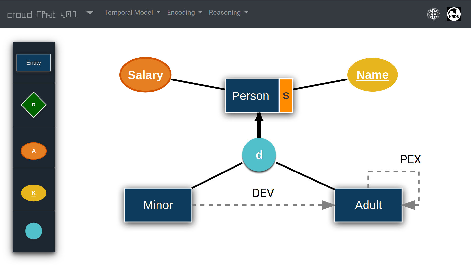
Figure 3: $\mathcal{ER_{VT}}$ graphical interface

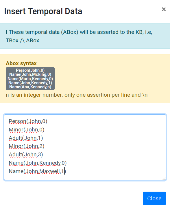
Figure 4: Widget to add temporal data

crowd-$\mathcal{ER_{VT}}$ supports temporal conceptual modelling in $\mathcal{ER_{VT}}$ providing a visual environment, a comprehensive set of $\mathcal{ER_{VT}}$ primitives, and an interface to off-the-shelf reasoners as depicted in Figure 2. Moreover, the tool provides an interface to add temporal data assertions (i.e., a temporal ABox) to populate the $\mathcal{ER_{VT}}$ model. Once both the $\mathcal{ER_{VT}}$ diagram and the temporal data have been specified, they are jointly sent to the server, where they are ultimately translated into LTL. When the reasoning process ends, the tool provides a link where the user can download the intermediate translations, including the TDL-Lite TBox and ABox encodings, the respective $\mathcal{QTL}_{1}$ translations, the encoding where past operators have been removed (if any), the final LTL formula, and the output of a reasoner.

To show how the tool works, we revisit the running examples introduced in Section 1 showing the corresponding $\mathcal{ER_{VT}}$ diagram, and the temporal data assertions. Figures 4 and 4 show the graphical interface extending Examples 1-2. In addition to the entities Person, Adult and Minor, and the attribute Name, the tool allows to specify visual marks for each temporal primitive in $\mathcal{ER_{VT}}$. For example, Person is set as a global entity (using the S mark, standing for Snapshot following the temporal ER notation [5] for global entities), while each Minor will become an Adult sometime in the future (expressed by the dotted line labeled DEV, standing for Dynamic EVolution). The axiom stating that minors and adults are disjoint is modelled as a disjoint composed ISA (the d labeled circle). The fact that every adult stays always adult in the future is captured by the dotted line labeled PEX (standing for Persistence). In Figure 4, we show the user interface to specify temporal assertions, showing the person John and his name at different timestamps.

The set of visual primitives also includes binary relationships (both global and local relationships are supported), and cardinalities are limited to the $1..1$ and $0..N$ cases. Cardinalities on attributes are limited to just $1..1$. Entities and attributes can be also tagged as global or local. Lastly, other forms of temporal operators between entities are also supported: TEX (standing for Transition EXtension) and DEX^- (standing for Dynamic EXtension) (see [2, 4, 5]).

5 Evaluation

Since there are no TDL-Lite ontologies available for testing, in our evaluation, we generated test ontologies synthetically, by extending methods applied in the context of propositional temporal logic [12]. We describe the test method in Subsection 5.1 and our results in Subsection 5.3.

5.1 The Test Method

We extend the test method proposed by Daniele, Giunchiglia, and Vardi [12] in the context of propositional temporal logic to our case. We analyse basic properties of the translation of TDL-Lite TBoxes into propositional temporal logic formulas. Following the mentioned method, we present two kinds of analyses.

• Average-behaviour: For a fixed number of $N$ concept names and of $N$ role names, a fixed maximum $Q$ for the value $q$ in basic concepts of the form $\geq qR$, a fixed number $L_{t}$ of CIs in a TBox, and for increasing values $L_{c}$ of the length of concept expressions in the TBox, we create batches $B(F,N,L_{t},L_{c},Q)$ of $F$ random TBoxes. We can then plot the results against $L_{c}$ and repeat the process for different values of $N$, $Q$, and $L_{t}$.

• Temporal-behaviour: For a fixed set of parameters $N,Q,L_{t},L_{c}$, and for increasing values of the probability $P_{t}$ of generating the temporal operators $\{\Diamond_{P},\Diamond_{F},\Box_{P},\Box_{F}\}$ and the probability $P_{g}$ of generating global roles, we create batches $B(F,N,L_{t},L_{c},Q,P_{t},P_{g})$ of $F$ random TBoxes. We can then plot the results against $P_{t}$ and $P_{g}$ and repeat the process for different values of $N$, $Q$, $L_{c}$, and $L_{t}$.

We now describe the procedure for generating random TDL-Lite TBoxes drawn uniformly from the space of TDL-Lite TBoxes with $L_{t}$ CIs and concept expressions with length $L_{c}$ (exactly $L_{t}$ and $L_{c}$, not up to $L_{t}$ and $L_{c}$). These concept expressions are formulated with concept and role names in $\{A_{1},\ldots,A_{N}\}$ and $\{R_{1},\ldots,R_{N}\}$, respectively, and $q\leq Q$ in basic concepts of the form $\geq qR$. Since there is no risk of confusion, in what follows we omit “uniformly”.

For the average-behaviour analysis, we proceed as follows. A random concept expression with length one is generated by randomly choosing a basic concept. Random concept expressions of length two are of the form ${\sf op}(C)$ where $C$ is a random concept expression with length one and ${\sf op}$ is randomly chosen from $U=\{\neg,\ocircle_{F},\ocircle_{P},\Diamond_{F},\Diamond_{P},\Box_{F},\Box_{P}\}$. For concept expressions with length $L$ larger than one, ${\sf op}$ is randomly chosen from $U\cup\{\sqcap\}$. If ${\sf op}\in U$ (that is, ${\sf op}$ is unary) then the random concept expression is ${\sf op}(C)$, where $C$ is a random concept expression with length $L-1$. Otherwise, we randomly choose $K$ in $\{1,\ldots,L-2\}$ and the random concept expression is $C\sqcap D$, where $C$, $D$ are random concept expressions with length $K$ and $L-K-1$, respectively. For the temporal-behaviour analysis we use the parameter $P_{t}$ to increase the chance of generating the temporal operators in $\{\Diamond_{F},\Diamond_{P},\Box_{F},\Box_{P}\}$ and the parameter $P_{r}$ increase the chance of generating a global role. Random concept expressions with length one are generated as for the average-behaviour analysis. For concept expressions with length two, the concept expression is of the form ${\sf op}(C)$, where the probability that ${\sf op}=\Diamond_{F}$ is $\frac{P_{t}}{4}$ (same for ${\sf op}$ being $\Diamond_{P},\Box_{F}$ or $\Box_{P}$) and the probability that ${\sf op}=\neg$ is $\frac{1-P_{t}}{3}$ (same for the other two unary operators). For concept expressions with length greater than two, ${\sf op}$ is again chosen from $U\cup\{\sqcap\}$ but now we have $\frac{1-P_{t}}{4}$ for the probability that ${\sf op}$ is $\neg$ (same for $\ocircle_{F},\ocircle_{P},\sqcap$). We have also generated ABoxes randomly, using the concept and role names occurring in TBoxes.

We are interested in investigating how different logical constructs of TDL-Lite TBoxes affect the size of the translation, the time for computing the translation, and the time for deciding satisfiability using tools designed for LTL. In the temporal-behaviour analysis, we want to study how the presence of temporal operators $\Diamond_{F},\Diamond_{P},\Box_{F},\Box_{P}$ and global roles affect the size of the translation and the time to compute the translation and to check for satisfiability.

5.2 Experimental environment and LTL solvers

We briefly present the hardware/software environment where the tests have been performed together with the off-the-shelf LTL solvers used.

Hardware and Software.

We run the experiments on a server with 8 Genuine Intel 3.6 GHz processors, and 4 GB memory running Debian GNU/Linux 10 (buster) with 64 bit kernel 4.19.0-8. Run time and memory usage were measured with runlim.

We set the run time to a timeout of 600 CPU seconds, while memory is set up to 1 GB. In the test, we denote with ‘T/O’ the case where the solver either runs out of memory or it times out. With ‘Fail’ we denote the case where the solver encountered an unexpected error condition.

LTL Solvers.

We considered various LTL solvers adopting different reasoning strategies: reduction to model checking, tableau-based algorithms, and temporal resolution. The chosen solvers have been already considered in the literature to test their performances for checking LTL formula satisfiability [27, 21]. As for the solvers based on model checking, we opted for NuXMV using the following options: BDDs (Binary Decision Diagrams), SAT (based on SAT techniques and also denoted as BMC for Bounded Model Checking), and the variant IC3 (known also as Property Directed Reachability) [11, 10, 13]. BDD is a complete satisfiability technique but it requires space exponential in the number of variables, and it is also sensitive to the variable order. On the other hand, BMC reduces the problem to SAT by testing the formula for satisfiability in models with length bounded by a fixed $k$, giving sound but incomplete results. IC3 computes approximations of reachability in a backward-search fashion.

The solver pltl [28] implements a tableau-based algorithms. We run pltl with the options graph and tree. Both methods build rooted trees with ancestor cycles but different search strategies (see also [19] for details). Compared with the traditional tableau-based translation, Aalta (Another Algorithm for LTL To Büchi Automata) [22], implements a new algorithm by introducing the concept of Obligation Set for LTL formulas. Aalta integrates two functions: LTL-to-Büchi translation and LTL satisfiability checking. Finally, TRP++UC [26] implements temporal resolution, and has been used with the option dfs/bfs (Depth-First search/Breadth-First search). This solver has been built on TRP++ [20]. Despite the aim of TRP++UC is to extract unsatisfiable cores for LTL, we used the legacy features of TRP++ by running the solver with the unsatisfiable cores option disabled.

5.3 Results

In what follows we evaluate the efficiency and the scalability of our tool using two evaluation tests of increasing difficulties. The first test is based on the toy scenarios described in Examples 1 and 2. The second test applies the test method for generating TBoxes randomly, as described in Subsection 5.1. Our benchmark is available from http://crowd.fi.uncoma.edu.ar/temporalDLLite/benchmark/. We discovered in our experimental evaluation that Aalta presents limitations when the LTL input has more than 1200 propositional variables.

5.3.1 Toy Scenarios Experiment.

We report here on the experimental results conducted by pairing the TBoxes of the toy examples, as reported in Section 1, with different ABoxes which may yield satisfiable (SAT) and unsatisfiable (UNSAT) KBs. The sizes of the ABoxes vary from $20$ to $50$ assertions (distributed over different time points). The number of propositional variables in the resulting LTL formula starts from a minimum of 14 variables, for the KB as in Example 1, and ranges from 180 to 2336 variables for Example 2 depending on the increasing sizes of the tested ABoxes. The experimental results for the cases where the TBox is as in Examples 1 and 2 are shown in Figures 5.3.1 and 5.3.1, respectively. For the UNSAT cases, we explicitly inserted inconsistent assertions (e.g., John being both Minor and Adult, in case of Example 1, while we added more than 1 name to the same person in case of Example 2). The results, presented in the form of ‘heat maps’, represent the runtime of the KB satisfiability checking for increasing ABox sizes (in columns) and different solvers (in lines).

	SAT	UNSAT
Aalta 0 pltl (graph) 0 pltl (tree) 0 NuXMV-BDD 0 NuXMV-SBMC 60 0 NuXMV-SBMC 20 0 NuXMV-IC3 0 TRP++(BFS) 0 TRP++(DFS) 0

& 4 4 4 4 4 4 4 4 4 4 4 4 4 4 4 4 4 4 4 4 4 4

Figure 5: Heat map with the runtimes for Example 1. Each rectangle represents the runtime in CPU seconds of SAT and UNSAT KBs with ABoxes of increasing size. The runtimes are given in colours as follows:

	$<\makebox[18.99995pt][r]{$0.01$}$ sec		$>\makebox[18.99995pt][r]{$0.01$}$ sec, $\leq\makebox[18.99995pt][r]{$0.25$}$ sec		$>\makebox[18.99995pt][r]{$0.25$}$ sec, $\leq\makebox[18.99995pt][r]{$0.50$}$ sec		$>\makebox[18.99995pt][r]{$0.50$}$ sec, $\leq\makebox[18.99995pt][r]{$1$}$ sec
	$>\makebox[18.99995pt][r]{$1$}$ sec, $\leq\makebox[18.99995pt][r]{$2$}$ sec		$>\makebox[18.99995pt][r]{$2$}$ sec, $\leq\makebox[18.99995pt][r]{$4$}$ sec		$>\makebox[18.99995pt][r]{$4$}$ sec, $\leq\makebox[18.99995pt][r]{$8$}$ sec		$>\makebox[18.99995pt][r]{$8$}$ sec, $\leq\makebox[18.99995pt][r]{$16$}$ sec
	$>\makebox[18.99995pt][r]{$16$}$ sec, $\leq\makebox[18.99995pt][r]{$32$}$ sec		$>\makebox[18.99995pt][r]{$32$}$ sec, $\leq\makebox[18.99995pt][r]{$64$}$ sec	0	$>\makebox[18.99995pt][r]{$64$}$ sec, $\leq\makebox[18.99995pt][r]{$125$}$ sec	1	$>\makebox[18.99995pt][r]{$125$}$ sec, $\leq\makebox[18.99995pt][r]{$250$}$ sec
2	$>\makebox[18.99995pt][r]{$250$}$ sec, $\leq\makebox[18.99995pt][r]{$500$}$ sec	3	$>\makebox[18.99995pt][r]{$500$}$ sec, $\leq\makebox[18.99995pt][r]{$1000$}$ sec	4	T/O, OoM or Fail

4	4	4	4
4	4	4	4
4	4	4	4
4
4	4	4	4
4	4	4	4

	0	4	4
4	4	4	4
4	4	4	4
4	4	4	4
4	4	4	4
4	4	4	4
4	4	4	4
4	4	4	4

Figure 6: Heat map with the runtimes of Example 2. Each rectangle represents the runtime in CPU seconds of SAT and UNSAT KBs with ABoxes of increasing size (the colours are as in the previous figure).

Solvers had better performances over SAT instances compared to UNSAT ones, except TRP++ which fails to scale even to small ABoxes. Moreover, NuXMV-SBMC fails regardless the size of the model in UNSAT cases (also when running in the simpler scenario of Example 1). Considering the experimental setting of Example 1 (Fig. 5.3.1), we note that the best performers over UNSAT cases were NuXMV with BDD and NuXMV with IC3, Aalta and pltl. The more involved setting of Example 2 clearly shows that the BMC option is the best for the SAT cases while NuXMV with the IC3 option stands out in the UNSAT case. Aalta performs well but only when the LTL input does not exceed $1200$ variables.

		0	1
1	1	2	4

4	4	4	4
4	4	4	4

4	4	4	4
4	4	4	4
	4

$L_{c}=5$

rien

$L_{c}=10$

rien

rien

rien

rien

rien

rien

rien

rien

rien

rien

rien

rien

rien

Figure 7: Heat map of the runtimes on randomly generated TBoxes according to the average behaviour (the colors are as in the toy experiments).

	0	1	2
	0	1	3

4	4	4	4
4	4	4	4

4	4	4	4
4	4	4	4

$L_{c}=5$

rien

$L_{c}=10$

rien

rien

rien

rien

rien

rien

rien

rien

rien

rien

rien

rien

rien

Figure 8: Heat map of the runtimes on randomly generated TBoxes according to the temporal behaviour (the colors are as in the toy experiments).

5.3.2 Randomly Generated TBoxes.

With this experiment setting we investigate the reasoning scalability over randomly generated TBoxes (see Section 5.1). These are KBs with an empty ABox and with (mostly) SAT TBoxes. In this is evaluation we only consider LTL solvers that performed well in the previous toy scenarios, namely, NuXMV-SBMC, Aalta, and NuXMV-IC3. Again, we use ‘heat maps’ to illustrate the obained results. For each solver, the results are reported in two consecutive lines: the first line denoting the case where $L_{c}=5$, while the second has $L_{c}=10$. Each square represents the runtime for different values of $N$ according to the following legenda:

• For the average behaviour, TBoxes were generated with the parameters $F=20$, $N=1,3,5$, $L_{t}=5,10,15,20$ (columns), $L_{c}=5,10$ (lines), and $Q=5$.

• For the temporal behaviour, TBoxes are generated with the parameters $F=20$, $N=1,3,5$, $L_{t}=10$, $L_{c}=5,10$ (lines), $Q=5$, $P_{t}=0.1,0.9$, and $P_{g}=0.7,0.9$ (the first two columns are with $P_{g}=0.7$ and two values for $P_{t}=0.1,0.9$, the last two columns are with $P_{g}=0.9$ and again $P_{t}=0.1,0.9$).

Concerning the number of propositional variables in the resulting LTL formulae and the current experimental setting, the average behaviour generated formulae from 400 and up to 8400 variables ($L_{c}$ = 5), and from 500 and up to 14500 variables ($L_{c}$ = 10). On the other hand, the temporal behaviour generated from 400 and up to 3500 variables ($L_{c}$ = 5), and from 950 and up to 6600 variables ($L_{c}$ = 10).

Due to the increase in the number of variables when removing the past operators, as expected solvers perform better on TBoxes expressed with only future operators (i.e., on $\textsl{T}^{\mathbb{N}}\textsl{DL-Lite}$ TBoxes) as shown on lines 3, 4 and 5 on both Figures 5.3.1 and 5.3.1, with the BMC option performing better than IC3. In the general case (presence of both past and future operators), the LTL translation that removes past operators at the cost of a linear increase of the propositional variables makes the reasoning more difficult. Moreover, there is not much difference between the heat map corresponding to the average behavior (Fig. 5.3.1) and the one of the temporal behavior (Fig. 5.3.1). In our experimental setting, this indicates that the LTL solvers were more affected by the number of propositional variables involved in the formula than by the number of temporal operators in the formula. Once again the BMC option is the best one for reasoning on SAT cases.

6 Conclusions

We illustrated the feasibility of automated reasoning on TDL-Lite KBs by leveraging existing off-the-shelf LTL reasoners. We tested both toy examples, where the addition of the ABox makes the toy KBs unsatisfiable, and randomly generated KBs. While the random tests gave a measure of the scalability and robustness of the off-the-shelf solvers while checking TBoxes satisfiability, the setting of the toy scenario was useful to check the behaviours of the solvers when dealing with ABoxes.

To summerize the discoveries, two major culprits in the runtime of solvers are the size of the ABox and the presence of past operators. While reasoners are not able to check formulas with past operators interpreted over the integers, eliminating past operators increases the number of propositional variables in a formula and this penalizes the runtime of the solvers. Better performances have been obtained when checking KBs with just future operators. Concerning ABoxes, the preliminary results show that a brute force approach makes reasoning in the presence of ABoxes almost unfeasable and different approaches need to be investigated.

Being the first attempt ever to check how LTL solvers deal with TDL-Lite KBs we foresee various open research directions to improve the results obtained here. On one side, one could aim at developing algorithms to deal directly with the DL/first-order case avoiding the LTL grounding that makes the size of the resulting LTL encoding not manageable, in particular, in the presence of ABoxes. How to deal with ABoxes is still open and current techniques embedded in DL reasoners dealing with real size ABox should be investigated. In this respect, we plan to extend to the temporal case the existing ABox abstraction approaches, which are successfully applied over OWL ontologies [14, 18].

References

- [1] A. Artale, D. Calvanese, R. Kontchakov, and M. Zakharyaschev. The DL-Lite family and relations. J. Artif. Intell. Res. (JAIR), 36(1):1–69, 2009.
- [2] A. Artale and E. Franconi. Temporal ER modeling with description logics. In Conceptual Modeling - ER ’99, 18th International Conference on Conceptual Modeling, Proceedings, pages 81–95, 1999.
- [3] A. Artale and E. Franconi. Temporal description logics. In Handbook of Temporal Reasoning in Artificial Intelligence, pages 375–388. Elsevier, 2005.
- [4] A. Artale and E. Franconi. Foundations of temporal conceptual data models. In A. Borgida, V. Chaudhri, P. Giorgini, and E. Yu, editors, Conceptual Modeling: Foundations and Applications, volume LNCS 5600 of Lecture Notes in Computer Science, pages 10–35. Springer, 2009. ISBN: 978-3-642-02462-7.
- [5] A. Artale, R. Kontchakov, V. Ryzhikov, and M. Zakharyaschev. Complexity of reasoning over temporal data models. In Proc. of the International Conference on Conceptual Modeling (ER-10), 2010.
- [6] A. Artale, R. Kontchakov, V. Ryzhikov, and M. Zakharyaschev. A cookbook for temporal conceptual data modelling with description logics. ACM Trans. Comput. Log., 15(3):25:1–25:50, 2014.
- [7] F. Baader, S. Ghilardi, and C. Lutz. LTL over description logic axioms. ACM Trans. Comput. Log., 13(3), 2012.
- [8] G. A. Braun, L. A. Cecchi, and P. R. Fillottrani. Taking advantages of automated reasoning in visual ontology engineering environments. In Proc. of the Joint Ontology Workshops 2019 Episode V: The Styrian Autumn of Ontology (JOWO’19), 2019.
- [9] G. A. Braun, C. Gimenez, L. A. Cecchi, and P. R. Fillottrani. crowd: A visual tool for involving stakeholders into ontology engineering tasks. Künstl Intell (2020), 2020.
- [10] R. Cavada, A. Cimatti, M. Dorigatti, A. Griggio, A. Mariotti, A. Micheli, S. Mover, M. Roveri, and S. Tonetta. The NuXMV symbolic model checker. In 26th Int. Conf. on Computer Aided Verification, (CAV), volume 8559 of Lecture Notes in Computer Science, pages 334–342. Springer, 2014.
- [11] A. Cimatti, E. Clarke, E. Giunchiglia, F. Giunchiglia, M. Pistore, M. Roveri, R. Sebastiani, and A. Tacchella. NuSMV 2: An opensource tool for symbolic model checking. In E. Brinksma and K. G. Larsen, editors, Computer Aided Verification, pages 359–364. Springer Berlin Heidelberg, 2002.
- [12] M. Daniele, F. Giunchiglia, and M. Y. Vardi. Improved automata generation for linear temporal logic. In CAV, 1999.
- [13] N. Een, A. Mishchenko, and R. Brayton. Efficient implementation of property directed reachability. In Proc. of the Int. Conf. on Formal Methods in Computer-Aided Design, FMCAD-11, page 125–134, 2011.
- [14] A. Fokoue, F. Meneguzzi, M. Sensoy, and J. Z. Pan. Querying linked ontological data through distributed summarization. In J. Hoffmann and B. Selman, editors, Proceedings of the Twenty-Sixth AAAI Conference on Artificial Intelligence. AAAI Press, 2012.
- [15] D. M. Gabbay. The declarative past and imperative future: Executable temporal logic for interactive systems. In B. Banieqbal, H. Barringer, and A. Pnueli, editors, Proceedings of the 1st Conference on Temporal Logic in Specification, volume 398 of Lecture Notes in Computer Science, page 409–448. Springer-Verlag, 1989.
- [16] D. M. Gabbay, A. Pnueli, S. Shelah, and J. Stavi. On the temporal analysis of fairness. In Conference Record of the 7th ACM Symposium on Principles of Programming Languages (POPL’80), page 163–173. ACM Press, 1980.
- [17] N. Gigante, A. Montanari, and M. Reynolds. A one-pass tree-shaped tableau for LTL+past. In T. Eiter and D. Sands, editors, LPAR-21, volume 46 of EPiC Series in Computing, pages 456–473, 2017.
- [18] B. Glimm, Y. Kazakov, and T. Tran. Scalable reasoning by abstraction beyond DL-Lite. In M. Ortiz and S. Schlobach, editors, Web Reasoning and Rule Systems (RR) - Proceedings of the 10th International Conference, volume 9898 of Lecture Notes in Computer Science, pages 77–93. Springer, 2016.
- [19] R. Goré and F. Widmann. An optimal on-the-fly tableau-based decision procedure for PDL-satisfiability. In R. A. Schmidt, editor, Automated Deduction, CADE-22, pages 437–452, 2009.
- [20] U. Hustadt and B. Konev. TRP++2.0: A temporal resolution prover. In Automated Deduction - CADE-19, 19th International Conference on Automated Deduction, Proceedings, pages 274–278, 2003.
- [21] U. Hustadt, A. Ozaki, and C. Dixon. Theorem proving for metric temporal logic over the naturals. In CADE, pages 326–343, 2017.
- [22] J. Li, S. Zhu, G. Pu, L. Zhang, and M. Y. Vardi. Sat-based explicit LTL reasoning and its application to satisfiability checking. Formal Methods Syst. Des., 54(2):164–190, 2019.
- [23] C. Lutz, F. Wolter, and M. Zakharyaschev. Temporal description logics: A survey. In Proc. of the 15th Int. Symposium on Temporal Representation and Reasoning, TIME’08, pages 3–14. IEEE Computer Society, 2008.
- [24] N. Markey. Temporal logic with past is exponentially more succinct. Bulletin of the EATCS, 79:122–128, 2003.
- [25] A. Poggi, D. Lembo, D. Calvanese, G. D. Giacomo, M. Lenzerini, and R. Rosati. Linking data to ontologies. J. of Data Semantics, 10:133–173, 2008.
- [26] V. Schuppan. Extracting unsatisfiable cores for LTL via temporal resolution. In C. Sánchez, K. B. Venable, and E. Zimányi, editors, 2013 20th International Symposium on Temporal Representation and Reasoning, Pensacola, FL, USA, September 26-28, 2013, pages 54–61. IEEE Computer Society, 2013.
- [27] V. Schuppan and L. Darmawan. Evaluating LTL satisfiability solvers. In Automated Technology for Verification and Analysis, 9th International Symposium, ATVA 2011. Proceedings, pages 397–413, 2011.
- [28] S. Schwendimann. A new one-pass tableau calculus for PLTL. In H. de Swart, editor, Automated Reasoning with Analytic Tableaux and Related Methods, pages 277–291. Springer Berlin Heidelberg, 1998.
- [29] G. Tseytin. On the complexity of derivation in propositional calculus. In Leningrad Seminar on Mathematical Logic, 1966.
- [30] M. Vigo, S. Bail, C. Jay, and R. D. Stevens. Overcoming the pitfalls of ontology authoring: Strategies and implications for tool design. Int. J. Hum. Comput. Stud., 72(12):835–845, 2014.