Spaceborne Synthetic Aperture Radar Imaging

Abstract

In this paper, we present the Spaceborne Synthetic Aperture Radar (SAR) imaging process for low squint angle case in stripmap mode. We describe the entire SAR image reconstruction procedure.

We then use experimental data gathered from RADARSAT-1 satellite of Vancouver, Canada and reconstruct the SAR image and show the results.

I Introduction

Radar is a day-night, all-weather and long range sensor which has been used for decades to sense the environment [1, 2]. Improving the ability of the radar in distinguishing the targets that have been located closely from one another has remained a challenge. To increase the resolution of the radar in the range direction the idea of pulse compression is utilized which nowadays is the most common technique used by all high resolution radars [1, 2]. The range resolution depends on the bandwidth of the transmitted signal and by increasing the bandwidth finer resolution in the range direction can be achieved.

The angular resolution, however, depends on the size of the antenna relative to the wavelength of the signal transmitted by the radar. To create higher angular resolution, we need to increase the size of the antenna relative to the wavelength of the transmitted signal. However, increasing the size of the antenna is not always an option as it is impossible to mount large antennas on board satellites or airplanes to conduct space based microwave imaging.

Synthetic Aperture Radar (SAR) imaging is a unique method to create the effect of a large real aperture synthetically. The high resolution in the azimuth direction in SAR imaging stems from the relative motion between the radar and the target [3, 4, 5, 6, 7]. In fact, the Doppler effect produced by the relative motion between the radar and the terrain to be imaged, will give rise to incredibly high resolution in the azimuth direction.

In this paper, we specifically consider the stripmap mode spaceborne SAR imaging in which the angle between the main axis of the antenna and the terrain to be imaged remains fixed [5, 4, 8]. As we mentioned before, when it comes to obtaining high resolution in the range direction, SAR uses the idea of pulse compression similar to the high resolution radars. A Linear Frequency Modulated (LFM) signal, a.k.a., chirp signal, is transmitted and the reflected signal is passed through matched filter and a high resolution profile in the range direction is produced [1, 2, 5, 4]. The resolution depends on the bandwidth of the chirp signal.

The interesting fact about SAR is that the relative motion between the radar and the target generates a chirp signal in the azimuth direction as well. Hence, similar to the range direction we can apply the idea of pulse compression in the azimuth direction and this way obtain a high resolution profile.

One of the features of the stripmap mode SAR imaging is the squint angle of the antenna which shifts the spectrum of the signal in the azimuth direction. For this reason, the signal in the azimuth direction is no longer at baseband. Nonzero squint angle is the main reason for Range Cell Migration (RCM) phenomenon which if it is not compensated for, it degrades the image quality in both the range and azimuth directions considerably.

The average value of the azimuth frequency is called the Doppler centroid frequency and it plays an important role in SAR image reconstruction. The best possible way to estimate the Doppler centroid frequency is by using the received data. Estimating the Doppler centroid frequency by analysing the geometry does not give rise to an accurate result since the location of the satellite cannot be estimated with high precision [5].

Since the sampling rate in the azimuth direction is equal to the Pulse Repetition Frequency (PRF), hence, if the Doppler centroid frequency exceeds the PRF, there will be ambiguity in its estimated value.

In this paper, we present spaceborne SAR image reconstruction operating in stripmap mode. The raw data used in this work has been gathered from RADARSAT-1 satellite [9] of Vancouver, Canada. To perform the SAR image reconstruction we utilize two well-known high resolution methods, namely, the Range Doppler and the Wavenumber algorithms.

The Range Doppler algorithm is the first algorithm that was developed for spaceborne SAR image reconstruction [10, 11, 12]. The Range Doppler algorithm is a compromise between accuracy and speed.

The Wavenumber algorithm [13, 14, 5], also referred to as $\omega-k$ algorithm and Range Migration Algorithm (RMA), is implemented in 2D frequency domain. Similar to the Range Doppler algorithm the Wavenumber algorithm is also considered a high resolution method for SAR image reconstruction.

Furthermore, we address the speckle noise reduction. Due to the coherent nature of the SAR imaging process, the speckle noise, which is a multiplicative noise, will be present and will degrade the quality of the reconstructed image considerably [5]. The surface roughness on the order of the signal wavelength causes speckle noise to appear.

The organization of the paper is as follows. In section II, we describe the system model. In section III, we present the Range Doppler algorithm. We have dedicated section IV to the Doppler centroid frequency estimation. Section V describes the Wavenumber Algorithm. In section VI, we describe speckle noise reduction procedure. Finally, in section VII, we apply the algorithms to the experimental data gathered from RADARSAT-1 satellite and show the results.

II Model Description

Fig. 1 shows the system model.

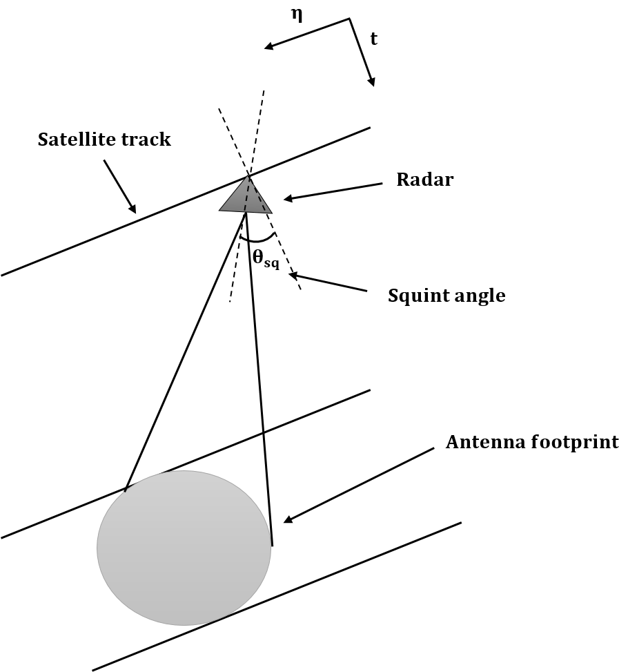
Figure 1: The model geometry.

The signal transmitted by the radar is a chirp signal described as

$$s(t)=w_{r}(t)e^{\displaystyle j2\pi f_{c}t+j\pi\beta t^{2}},$$ (1)

where $f_{c}$ is the carrier frequency and the parameter $\beta$ is given as $B/T$, in which $B$ and $T$ represent the bandwidth and the chirp time, respectively. In addition, $w_{r}$ is a rectangular window with length $T$ and $t$ is referred to as fast time variable.

The signal received at the location of the receiver, after being reflected by a point reflector, is a chirp signal modeled as

$$s(t,\eta)=\sigma\;w_{r}(t-\frac{2R(\eta)}{c})w_{a}(\eta-\eta_{c})\times$$

$$e^{\displaystyle j2\pi f_{c}(t-\frac{2R(\eta)}{c})+j\pi\beta{(t-\frac{2R(\eta)}{c})}^{2}},$$ (2)

where $\sigma$ is the complex reflection coefficient for the point reflector, $\eta$ is referred to as slow time variable and $R(\eta)$ is the distance from the radar to the target and is given as $R(\eta)=\sqrt{R^{2}_{0}+v^{2}{\eta}^{2}}$. Moreover, $w_{a}$ is a rectangular window which its length is equal to the synthetic aperture length divided by $v$ that is the speed of the satellite.

After down-conversion and ignoring the $e^{j\pi\beta{(\frac{2R(\eta)}{c})}^{2}}$ term, we can write (II) as

$$s(t,\eta)=\sigma\;w_{r}(t-\frac{2R(\eta)}{c})w_{a}(\eta-\eta_{c})$$

$$e^{\displaystyle-j4\pi f_{c}\frac{R(\eta)}{c}+j\pi\beta t^{2}-j4\pi\beta t\frac{R(\eta)}{c}}.$$ (3)

The ultimate goal in SAR imaging is to estimate the complex reflection coefficient $\sigma$. In the next section, we will describe the image reconstruction procedure.

III Range Doppler Algorithm

The Range Doppler algorithm is the first algorithm that was developed for spaceborne SAR image reconstruction [10, 11, 12]. The first step in the Range Doppler algorithm is to compress the energy of the target in the range direction. To accomplish this goal, we should perform matched filtering process. The matched filter is described as

$$s_{\rm mr}(t)=w_{r}(t)e^{\displaystyle-j\pi\beta t^{2}}.$$ (4)

Range compression based on (4) can be performed either in the time or in the frequency domain. We will perform the matched filtering in the frequency domain using FFT which is expressed as

$$s_{\rm rc}(t,\eta) =IFFT_{f_{t}}\{FFT_{t}(s(t,\eta))\bigodot FFT_{t}(s_{\rm mr}(t))\}$$ (5)

$$=\sigma\;p_{r}(t-\frac{2R(\eta)}{c})w_{a}(\eta-\eta_{c})e^{\displaystyle-j4\pi f_{c}\frac{R(\eta)}{c}},$$

where $p_{r}(.)$ is the Sinc function and $\bigodot$ stands for Hadamard product which is an element-wise product. Also, $f_{t}$ represents the fast time frequency. The Fourier transform is calculated analytically using the Method of Stationary Phase (MOSP) [15].

According to (5), after range compression process, the energy of the signal is localized in the range direction. The resolution in the range direction depends on the bandwidth of the transmitted signal and is given as $\delta R=\frac{c}{2B}$. The higher the bandwidth, the sharper the mainlobe of $p_{r}$ which subsequently results in finer range resolution.

The next step in the Range Doppler algorithm is to compress the energy of the signal, given in (5), in the azimuth direction. However, the argument of $p_{r}$ in (5) depends on the parameter $\eta$ which creates displacement in the range direction. In other words, the energy of the point reflector spreads over the neighboring range cells for different values of $\eta$. This is the RCM phenomenon.

Therefore, before performing the azimuth compression, we should perform the fast time and slow time decoupling of the signal given in (5) and compensate for the RCM effect. To set the stage, we use paraxial approximation which we are allowed to since in this paper we are considering the low squint angle case [5]. We will explain the effect of the squint angle on the image reconstruction procedure in the subsequent sections.

Consequently, we write $R(\eta)$ as $R(\eta)=R_{0}+\frac{v^{2}{\eta}^{2}}{2R_{0}}$ which as a result allows us to express (5) as

$$s_{\rm rc}(t,\eta) =\sigma\;p(t-\frac{2R(\eta)}{c})w_{a}(\eta-\eta_{c})\times$$ (6)

$$e^{\displaystyle-j4\pi f_{c}\frac{R_{0}}{c}-j\pi K_{a}{\eta^{2}}},$$

where $K_{a}=\frac{2v^{2}}{\lambda R_{0}}$.

Then, we take a Fourier transform from (6) with respect to $\eta$ which upon performing the Fourier transform using MOSP we obtain the following

$$S_{\rm rc}(t,f_{\eta}) =\sigma\;p(t-\frac{2R_{0}}{c}-\frac{\lambda^{2}R_{0}f^{2}_{\eta}}{8v^{2}})W_{a}(f_{\eta}-f_{\eta_{c}})\times$$ (7)

$$e^{\displaystyle-j4\pi f_{c}\frac{R_{0}}{c}}\;e^{\displaystyle j\pi\frac{f^{2}_{\eta}}{K_{a}}}.$$

In (7), the parameter $f_{\eta}$ represents the slow time frequency or the azimuth frequency. The signal given in (7) is in the range Doppler domain. The term related to the RCM is $\frac{\lambda^{2}R_{0}f^{2}_{\eta}}{8v^{2}}$ which depends on both $R_{0}$ and $f_{\eta}$. Therefore, the range Doppler domain can precisely compensate for the RCM using interpolation technique [16, 17, 18].

However, if we ignore the dependency of the RCM on $R_{0}$ and take a Fourier transform from (7) with respect to the fast time variable, the RCM will then appear as a phase term which can be easily removed. This second approach has the benefit of simplicity and speed over the interpolation in the range Doppler domain. The Fourier transform of (7) with respect to the fast time variable (using MOSP) results in

$$S_{\rm rc}(f_{t},f_{\eta}) =\sigma\;W_{r}(f_{t}-\frac{2R_{0}}{c})W_{a}(f_{\eta}-f_{\eta_{c}})\times$$ (8)

$$e^{\displaystyle-j2\pi f_{t}\frac{\lambda^{2}R_{0}f^{2}_{\eta}}{8v^{2}}}\;e^{\displaystyle-j4\pi f_{c}\frac{R_{0}}{c}}\;e^{\displaystyle j\pi\frac{f^{2}_{\eta}}{K_{a}}}.$$

Consequently, the task of RCM compensation is to remove the first phase term in (8). The RCM compensation in the 2D frequency domain is faster than performing it through interpolation in the range Doppler domain. However, as we mentioned before, performing RCM compensation using interpolation in the range Doppler domain is the most accurate method due to the dependency of RCM on both the range of the target as well as the Doppler frequency.

After RCM compensation and taking an inverse Fourier transform with respect to the fast time variable using MOSP, the signal can be represented in the range Doppler domain as

$$S_{\rm rcmc}(t,f_{\eta}) =\sigma\;p_{r}(t-\frac{2R_{0}}{c})W_{a}(f_{\eta}-f_{\eta_{c}})\times$$ (9)

$$e^{\displaystyle-j4\pi f_{c}\frac{R_{0}}{c}}\;e^{\displaystyle j\pi\frac{f^{2}_{\eta}}{K_{a}}}.$$

The final step for image formation in the Range Doppler algorithm is to compress the data in the azimuth direction. To perform the azimuth localization, we use the following matched filter

$$s_{\rm ma}(\eta) =w_{a}(\eta-\eta_{c})e^{\displaystyle j\pi K_{a}\eta^{2}}.$$ (10)

After performing matched filtering in the frequency domain by using FFT, we obtain the compressed signal in the range and azimuth directions as

$$s_{\rm rcac}(t,\eta)=IFFT_{f_{\eta}}\{S_{\rm rcmc}(t,f_{\eta})\}\bigodot FFT_{\eta}(s_{\rm ma}(\eta))$$

$$=\sigma\;p_{r}(t-\frac{2R_{0}}{c})p_{a}(\eta)e^{\displaystyle-j4\pi f_{c}\frac{R_{0}}{c}}\;e^{\displaystyle j2\pi f_{\eta_{c}}\eta},$$ (11)

where $f_{\eta_{c}}$ is the Doppler centroid frequency which we explain its meaning as well as methods to estimate it in the next section. The Fourier and inverse Fourier transforms in (III) have been calculated analytically based on MOSP.

IV Doppler Centroid Estimation

In the case of nonzero squint angle, the signal in the azimuth direction is no longer a baseband signal. In other words, the center of the spectrum is not at zero Doppler frequency.

The average value of the Doppler frequency is called the Doppler centroid frequency.

The Doppler centroid frequency $f_{\eta_{c}}$ corresponds to the slow time $\eta_{c}$ at which the target is at the center of the mainlobe of the antenna and hence, it receives the maximum energy from the radar.

Estimating the Doppler centroid frequency can be performed either through the geometry of the problem or using the data. In the case of spaceborne SAR imaging, due to the lack of accuracy in estimating the location of the satellite the Doppler centroid frequency estimation is mainly performed based on the received data.

Since the sampling rate in the azimuth direction is equal to the PRF, therefore, if the Doppler centroid frequency exceeds the PRF, there will be ambiguity in its estimated value. In fact, we can write

$$f_{dc} =M\times PRF+f^{\prime}_{dc}\;\;\;M\in\mathbb{Z},$$ (12)

where $-\frac{PRF}{2}\leq f^{\prime}_{dc}\leq\frac{PRF}{2}$. The Doppler centroid frequency depends on the distance between the radar and the target as well as the velocity of the satellite.

The slant range distance from the radar to the target can be Taylor expanded as [19]

$$R(\eta)=R(\eta_{c})+\frac{dR(\eta)}{d\eta}|_{\eta=\eta_{c}}(\eta-\eta_{c})$$ (13)

$$+\frac{1}{2}\frac{d^{2}R(\eta)}{d\eta^{2}}|_{\eta=\eta_{c}}(\eta-\eta_{c})^{2}.$$

From (13), the Doppler centroid frequency $f_{dc}$ is given as

$$f_{dc}=\frac{2}{\lambda}\frac{dR(\eta)}{d\eta}|_{\eta=\eta_{c}}=\frac{2}{\lambda}\frac{v^{2}\eta_{c}}{R(\eta_{c})}.$$ (14)

The third term in (13) is called the FM rate in the slow time direction and is expressed as

$$f_{R}=\frac{d^{2}R(\eta)}{d\eta^{2}}|_{\eta=\eta_{c}}=\frac{v^{2}R^{2}_{0}}{R^{3}(\eta_{c})}.$$ (15)

From (13), it is implied that the signal in the azimuth direction is a non-baseband chirp signal.

The fact that the relative motion between the satellite and the target creates a chirp signal in the azimuth direction is the reason for achieving high resolution in this direction.

There are different techniques for the Doppler centroid frequency estimation and they are divided into two different categories, namely, amplitude based and phased based methods [5].

The amplitude based spectral fit algorithm and phase based Average Cross Correlation Coefficient (ACCC) method are among two well-known methods for estimating $f^{\prime}_{dc}$ [5, 20].

The fractional part of the Doppler centroid frequency is what we need for the azimuth compression process. However, to compensate for the effect of the RCM we need the unwrapped Doppler centroid frequency. In other words, we need to estimate the unambiguous value of the Doppler centroid frequency.

Multilook Cross Correlation (MLCC) [5], Wavelength Diversity Algorithm (WDA) [21] and Multilook Beat Frequency (MLBF) technique [22, 23, 5] are among the methods that are used for estimating the unambiguous value of the Doppler centroid frequency. These three techniques are all phased based methods.

In the case of having strong isolated targets in the scene, the unambiguous Doppler centroid frequency can be found by estimating the slope of the range compressed data for the isolated targets.

V Wavenumber Algorithm

In this section, we present the Wavenumber algorithm [13, 14, 5], a.k.a., $\omega-k$ algorithm and Range Migration Algorithm (RMA). Similar to the Range Doppler algorithm, the Wavenumber algorithm is also considered as a high resolution method for SAR image reconstruction.

In the Wavenumber algorithm, the range compression, the RCM compensation as well as the azimuth localization are all performed in the 2D frequency domain.

The first task in implementing the Wavenumber algorithm is to take a 2D Fourier transform from (II) which by using MOSP we obtain the following

$$S(f_{t},f_{\eta})=\sigma\;W_{r}(f_{t})W_{a}(f_{\eta}-f_{\eta_{c}})\times$$ (16)

$$e^{\displaystyle-j4\pi\frac{R_{0}}{c}\sqrt{(f_{c}+f_{t})^{2}-\frac{c^{2}f^{2}_{\eta}}{4v^{2}}}-j\frac{\pi f^{2}_{t}}{\beta}},$$

where $f_{t}$ and $f_{\eta}$ are the fast time and slow time frequency variables, respectively. The last term in the phase of (16) is removed by multiplying the signal by $e^{j\frac{\pi f^{2}_{t}}{\beta}}$. We then multiply (16) by the reference phase function defined as

$$S_{\rm ref}(f_{t},f_{\eta})=e^{\displaystyle j4\pi\frac{R_{\rm ref}}{c}\sqrt{(f_{c}+f_{t})^{2}-\frac{c^{2}f^{2}_{\eta}}{4v^{2}}}},$$ (17)

which as a result, we obtain

$$S_{c}(f_{t},f_{\eta})=\sigma\;W_{r}(f_{t})W_{a}(f_{\eta}-f_{\eta_{c}})\times$$ (18)

$$e^{\displaystyle-j4\pi\frac{R_{0}-R_{\rm ref}}{c}\sqrt{(f_{c}+f_{t})^{2}-\frac{c^{2}f^{2}_{\eta}}{4v^{2}}}}.$$

For a target located at $R_{\rm ref}$ the phase component in (18) is removed completely and upon taking an inverse 2D Fourier transform we will localize the energy of the target in both the range and azimuth directions.

For the targets located at ranges other than $R_{\rm ref}$, however, there is a residual phase term in (18).

The next step in the Wavenumber algorithm is to linearize the phase term given in (18) which is performed using the Stolt interpolation [14, 13, 5]. The Stolt interpolation procedure is given as $\sqrt{(f_{c}+f_{t})^{2}-\frac{c^{2}f^{2}_{\eta}}{4v^{2}}}\rightarrow f_{c}+f^{\prime}_{t}$. After performing the Stolt interpolation, we obtain

$$S_{\rm cs}(f^{\prime}_{t},f_{\eta})= \sigma\;W_{r}(f^{\prime}_{t})W_{a}(f_{\eta}-f_{\eta_{c}})\times$$

$$e^{\displaystyle-j4\pi\frac{R_{0}-R_{\rm ref}}{c}(f_{c}+f^{\prime}_{t})}.$$

Finally, by taking a 2D inverse Fourier transform from (V) using MOSP, we localize the energy of the target in both the range and azimuth directions as

$$s_{c}(t,\eta)=\sigma\;p_{r}(t-2\frac{R_{0}-R_{\rm ref}}{c})p_{a}(\eta)\times$$

$$e^{\displaystyle j2\pi f_{\eta_{c}}\eta}\;e^{\displaystyle-j4\pi\frac{R_{0}-R_{\rm ref}}{c}f_{c}},$$ (20)

which represents the reconstructed image.

In the Wavenumber algorithm, the RCM compensation is performed in the 2D frequency domain. Therefore, the dependency of the RCM on the range variable is ignored. Performing the RCM in the 2D frequency domain instead of the range Doppler domain is a compromise between speed and accuracy.

Of course, as we mentioned before, even in the Range Doppler algorithm the RCM compensation can be performed in the 2D frequency domain using (8). We should also mention that the range dependency can be ignored for the case of low squint angle and small swath width.

VI Speckle Noise

When the terrain to be imaged is rough on the scale of the wavelength of the incident wave, then speckle noise appears. Speckle noise is a multiplicative noise. In fact, the origin of the speckle noise is the dependency of the relative phase of the individual reflectors inside the resolution cell on the viewing angle [5].

A very well-known method for speckle noise reduction is multi-look processing in which the synthetic aperture is divided into several independent parts and per each part an image from the scene is created [5]. The final image is the summation of the absolute value of the images created from the sub-apertures.

The major problem with the multi-look processing is that the resolution reduces due to using only a small portion of the aperture to create each independent image from the scene.

In this section, we present a filtering approach over the reconstructed image to reduce the effect of the speckle noise. We use the entire synthetic aperture to reconstruct the image. Therefore, there is no loss in the image resolution.

We introduce a 2D $m\times n$ filter and slide it over the reconstructed image while solving the following optimization problem,

$$\!\min_{a} \sum_{i=1}^{n}\sum_{j=1}^{m}|a_{ij}-a|,$$ (21)

where $a_{ij}$ is the value for the $(ij)^{\rm th}$ pixel and $a$ is the value chosen by the optimization problem for the $(\lfloor\frac{n-1}{2}\rfloor+1\;\lfloor\frac{m-1}{2}\rfloor+1)^{\rm th}$ pixel. In fact, by solving the optimization problem in (21) we are filtering the image by the median filter. In other words, we replace the value of each pixel with the median of the neighboring pixels.

VII experimental results

In this section, we present the result of SAR image reconstruction based on experimental data gathered from RADARSAT-1 satellite of Vancouver, Canada. The total data collection has taken 15 seconds.

The specifications for RADARSAT-1 have been given in Table.I.

TABLE I: RADARSAT-1’s Parameters

Parameters		Values
Center frequency($\rm GHz$)	$\rm f_{c}$	$5.3$
Radar sampling rate($\rm MHz$)	$\rm Fr$	$32.317$
Pulse repetition frequency($\rm Hz$)	$\rm PRF$	$1256.98$
Slant range of first radar sample($\rm km$)	$R_{0}$	$988.65$
FM rate of radar pulse($\rm MHz/\mu s$)	$\rm\beta$	$0.72135$
Chirp duration($\rm\mu s$)	$\rm Tr$	$41.75$
satellite velocity($\rm m/s$)	$\rm v$	$7062$
Bandwidth($\rm MHz$)	$\rm B$	$30.116$

First, we select the data from English Bay since there are several ships in this scene that play the role of isolated strong reflectors which will help to see the effect of the RCM clearly.

We start with the Range Doppler algorithm. Fig. 2 shows the range compressed data based on (6). The range compressed energy of the ships can be seen as a few skewed vertical lines. The skewness demonstrates the effect of the RCM phenomenon.

Another important information that we can obtain from Fig. 2 is that the satellite is moving backward with respect to the scene because the distance between the satellite and the targets increases when the satellite is moving in the azimuth direction. For this reason, the sign of the Doppler centroid frequency is negative.

In the Range Doppler algorithm, the next task following the range compression, is the RCM compensation. To accomplish this goal, we need the Doppler centroid frequency.

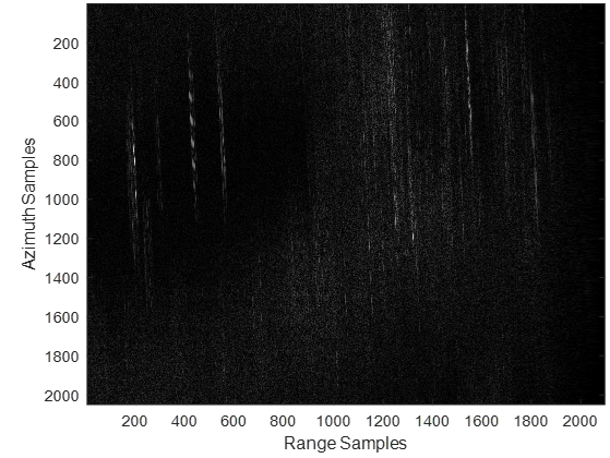
Figure 2: The result of applying (6) to the raw data and obtaining the range compressed signal.

As we mentioned before, if the Doppler centroid frequency is larger than the PRF of the RADAR, there will be an ambiguity in the Doppler centroid frequency estimation. In fact, according to (12), in order to be able to calculate the unambiguous Doppler centroid frequency we need to estimate $M$ as well as $f^{\prime}_{dc}$.

We first estimate the fractional part of the Doppler centroid frequency which is $f^{\prime}_{dc}$. Fig. 3 illustrates the power spectrum of the data in the azimuth direction versus the slow time frequency variable, $f_{\eta}$. In order to reduce the effect of the noise we have added the power spectrum corresponding to $230$ range cells. A sinusoidal signal has been fitted to the result.

From Fig. 3, we can easily estimate the fractional part of the Doppler centroid frequency as $f^{\prime}_{dc}=471Hz$ which is the frequency at which the power spectrum reaches its maximum.

For the azimuth compression process, the fractional part of the Doppler centroid frequency is enough. However, as we mentioned before, for RCM compensation we need to estimate the unwrapped value of the Doppler centroid frequency.

Thus, the next step is to estimate $M$ in (12).

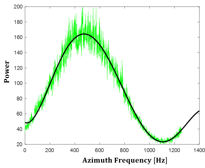
Figure 3: Estimating the fractional part of the Doppler centroid frequency.

One way to estimate the unwrapped value for the Doppler centroid frequency is by analysing the trajectory of strong isolated targets in the scene. Fig. 4 shows a blow-up part of the range compressed image shown in Fig. 2 related to a few stationary ships in water.

The skewness in the trajectory of these targets is due to the nonzero Doppler centroid frequency. The energy of each one of them is spread over several different range cells.

The slope can easily be calculated and is equal to $0.034$ range samples per azimuth samples. To estimate the Doppler centroid frequency we should first multiply the slope by $\frac{c}{2F_{r}}$ to convert the slope from range samples to range distance and then multiply it by the $\rm PRF$ to convert it from azimuth samples to azimuth time.

Hence, we have $\frac{dR(\eta)}{d\eta}=198.23m/s$. As a result, from (14) the Doppler centroid frequency can be calculated as $f_{dc}=-7009Hz$. The negative sign is realized from Fig. 2 which shows that the satellite is moving backward with respect to the scene while it is collecting the data.

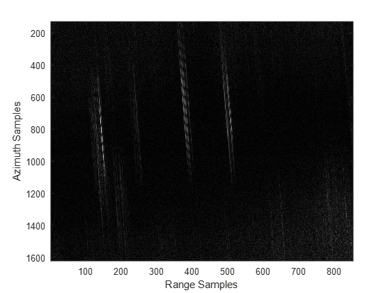
Figure 4: The blow-up part of Fig. 2 which shows the range compressed result for a few strong isolated targets.

Fig. 5 shows the result of the RCM compensation process. As can be seen from Fig. 5, the energy of the targets have been localized in their corresponding range cells.

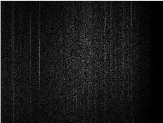
Figure 5: The result of the range compressed signal after RCM compensation.

Finally, the last stage is to perform the azimuth localization process. As a result, the reconstructed image based on the Range Doppler algorithm is obtained which has been shown in Fig. 6.

Next, we apply the Wavenumber algorithm to a different part of the raw data. We have shown the result in Fig. 7.

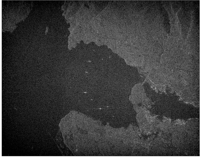
Figure 6: The reconstructed image of English Bay based on the Range Doppler algorithm.

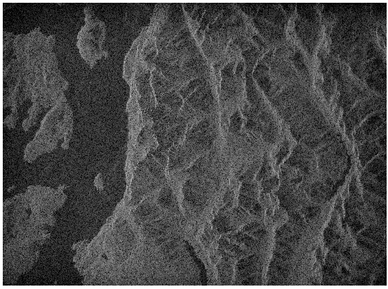
Figure 7: The reconstructed image based on the Wavenumber algorithm.

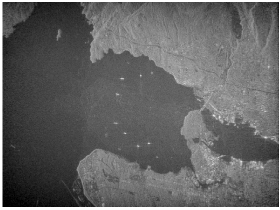
Figure 8: The result of speckle noise reduction for the reconstructed image shown in Fig. 6.

After the image reconstruction is completed, we will then focus on the speckle noise removal procedure based on (21). Fig. 8 shows the result of speckle noise reduction for the reconstructed image depicted in Fig. 6. To perform the speckle noise reduction, we have chosen $m=n=6$ for the filter given in (21).

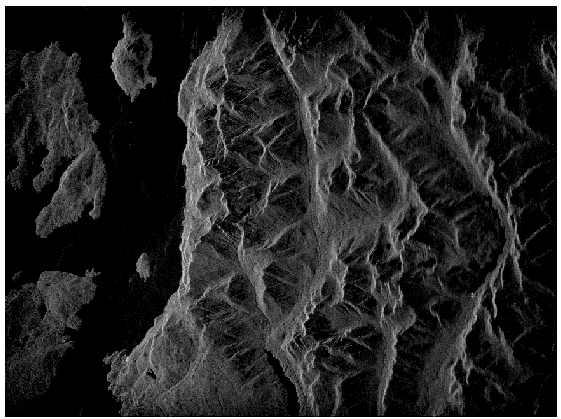
Figure 9: The result of speckle noise reduction for the reconstructed image shown in Fig. 7.

We have also applied the filtering process given in (21) to the image reconstructed by the Wavenumber algorithm shown in Fig. 7 and have illustrated the result in Fig. 9. To perform the speckle noise reduction, we have chosen the similar parameters for the filter, $m=n=6$.

Fig. 10 shows the result of applying the Range Doppler algorithm to a larger part of the raw data. To reduce the effect of the speckle noise we have applied the filter given in (21) with $m=n=10$.

VIII conclusion

In this paper, we presented the sapceborne SAR imaging process based on two well-known high resolution algorithms, namely, the Range Doppler and the Wavenumber algorithms. We discussed different parts of each algorithm in detail. Moreover, we addressed the speckle noise removal procedure.

Finally, we applied both algorithms to the experimental data gathered from RADARSAT-1 and showed the results.

Shahrokh Hamidi was born in Sanandaj, Kurdistan, Iran, in 1983. He received his B.Sc., M.Sc. and Ph.D. degrees all in Electrical and Computer Engineering.

SAFEDDIN SAFAVI-NAEINI was born in Gachsaran, Iran, in 1951. He received the B.Sc. degree in electrical engineering from the University of Tehran, Tehran, Iran, in 1974, and the M.Sc. and Ph.D. degrees in electrical engineering from the University of Illinois, Urbana Champaign, in 1975 and 1979, respectively. He joined the Department of Electrical and Computer Engineering, University of Tehran, as an Assistant Professor, in 1980, where he became an Associate Professor, in 1988. In 1996, he joined the Department of Electrical and Computer Engineering, University of Waterloo, ON, Canada, where he is currently a Full Professor and the RIM/NSERC Industrial Research Chair of intelligent radio/antenna and photonics. He is also the Director of a newly established Center for Intelligent Antenna and Radio System (CIARS). He has published over 80 journal papers and 200 conference papers in international conferences. His research activities deal with RF/microwave technologies, smart integrated antennas and radio systems, mmW/THz integrated technologies, nano-EM and photonics, EM in health sciences and pharmaceutical engineering, antenna, wireless communications and sensor systems and networks, new EM materials, bio-electro-magnetics, and computational methods. He has led several international collaborative research programs with research institutes in Germany, Finland, Japan, China, Sweden, and USA.

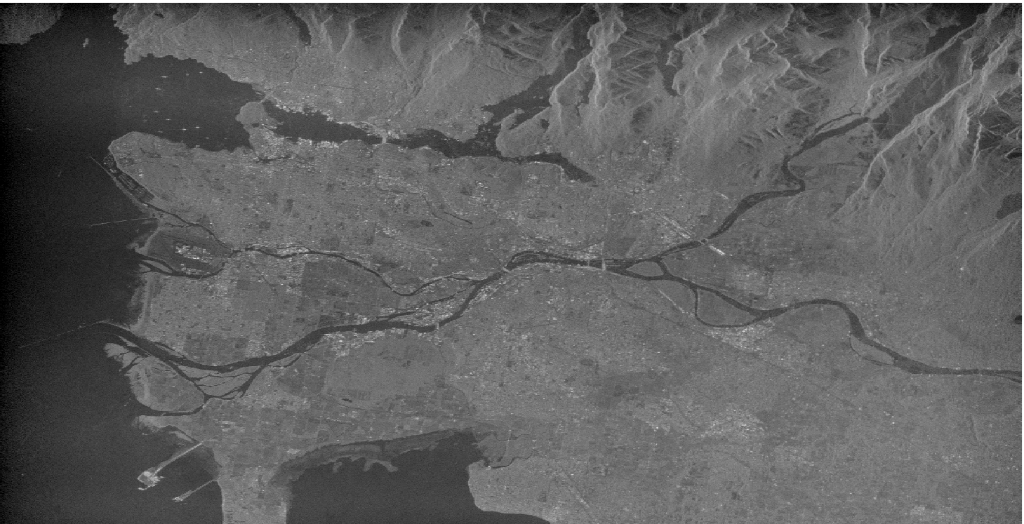
Figure 10: The reconstructed image of Vancouver, Canada based on the Range Doppler algorithm.

References

- [1] M. I. Skolnik, Introduction to Radar Systems. McGraw-Hill, New York, 2002.
- [2] B. R. Mahafza, Radar Systems Analysis and Design Using MATLAB. Chapman and Hall/CRC Press, Boca Raton, FL, 2000.
- [3] J. Curlander and R. McDonough, Synthetic Aperture Radar Systems and Signal Processing. John Wiley and Sons, New York, 1991.
- [4] M. Soumekh, Synthetic aperture radar signal processing with MATLAB algorithms. John Wiley, 1999.
- [5] I. G. Cumming and F. H. Wong, Digital processing of synthetic aperture radar data. Artech House, Norwood, MA, 2005.
- [6] R. O. Harger, Synthetic Aperture Radar Systems: Theory and Design. Academic Press, New York, 1970.
- [7] R. J. Sullivan, Microwave Radar Imaging and Advanced Concepts. Artech House, Norwood, MA, 2000.
- [8] D. Munson, “An introduction to strip-mapping synthetic aperture radar,” vol. 12, pp. 2245–2248, 1987.
- [9] R. K. Raney, A. P. Luscombe, E. J. Langham, and S. Ahmed, “RADARSAT SAR imaging,” Proceedings of the IEEE, vol. 79, no. 6, pp. 839–849, 1991.
- [10] I. Cumming and J. Bennett, “Digital processing of seasat SAR data,” vol. 4, pp. 710–718, 1979.
- [11] C. Chen and H. C. Andrews, “Target-motion-induced radar imaging,” IEEE Transactions on Aerospace and Electronic Systems, vol. AES-16, no. 1, pp. 2–14, 1980.
- [12] J. L. Walker, “Range-Doppler imaging of rotating objects,” IEEE Transactions on Aerospace and Electronic Systems, vol. AES-16, no. 1, pp. 23–52, 1980.
- [13] I. G. Cumming, Y. L. Neo, and F. H. Wong, “Interpretations of the omega-K algorithm and comparisons with other algorithms,” vol. 3, pp. 1455–1458, 2003.
- [14] R. Bamler, “A comparison of Range-Doppler and wavenumber domain SAR focusing algorithms,” IEEE Transactions on Geoscience and Remote Sensing, vol. 30, no. 4, pp. 706–713, 1992.
- [15] M. Born and E. Wolf., Principles of Optics. Cambridge University Press, Cambridge, England, 7th edition, 1999.
- [16] M. Soumekh, “Band-limited interpolation from unevenly spaced sampled data,” IEEE Transactions on Acoustics, Speech, and Signal Processing, vol. 36, no. 1, pp. 110–122, 1988.
- [17] L. Lidicky and P. Hoogeboom, “A fast algorithm to compute band-limited interpolation from unevenly spaced sampled data using k-nearest neighbor search,” pp. 4 pp.–, 2006.
- [18] G. Lee, “Nonlinear interpolation,” IEEE Transactions on Information Theory, vol. 17, no. 1, pp. 45–49, 1971.
- [19] F. k. Li and W. T. K. Johnson, “Ambiguities in spacebornene synthetic aperture radar systems,” IEEE Transactions on Aerospace and Electronic Systems, vol. AES-19, no. 3, pp. 389–397, 1983.
- [20] S. N. Madsen, “Estimating the Doppler centroid of sar data,” IEEE Transactions on Aerospace and Electronic Systems, vol. 25, no. 2, pp. 134–140, 1989.
- [21] R. Bamler and H. Runge, “PRF-ambiguity resolving by wavelength diversity,” IEEE Transactions on Geoscience and Remote Sensing, vol. 29, no. 6, pp. 997–1003, 1991.
- [22] I. G. Cumming and S. Li, “Adding sensitivity to the MLBF Doppler centroid estimator,” IEEE Transactions on Geoscience and Remote Sensing, vol. 45, no. 2, pp. 279–292, 2007.
- [23] Shu Li and I. Cumming, “Improved beat frequency estimation in the MLBF Doppler ambiguity resolver,” vol. 5, pp. 3348–3351, 2005.