Central exclusive diffractive production of axial-vector $f_{1}(1285)$ and $f_{1}(1420)$ mesons in proton-proton collisions

Abstract

We present a study of the central exclusive diffractive production of the $f_{1}(1285)$ and $f_{1}(1420)$ resonances in proton-proton collisions. The theoretical results are calculated within the tensor-pomeron approach. Two pomeron-pomeron-$f_{1}$ tensorial couplings labeled by $(l,S)=(2,2)$ and $(4,4)$ are derived. We adjust the model parameters (coupling constants, cutoff constant) to the WA102 experimental data taking into account absorption effects. Both the $(l,S)=(2,2)$ and $(4,4)$ couplings separately allow one to describe the WA102 differential distributions. We compare these predictions with those of the Sakai-Sugimoto model, where the pomeron-pomeron-$f_{1}$ couplings are determined by the mixed axial-gravitational anomaly of QCD. We derive an approximate relation between the pomeron-pomeron-$f_{1}$ coupling constants of this approach and the $(l,S)=(2,2)$ and $(4,4)$ couplings. Then we present our predictions for the energies available at the RHIC and LHC. The total cross sections and several differential distributions are presented. Analysis of the distributions in the azimuthal angle $\phi_{pp}$ between the transverse momenta of the outgoing protons may be used to disentangle $f_{1}$- and $\eta$-type resonances contributing to the same final channel. We find for the $f_{1}(1285)$ a total cross section $\sim 38$ $\mu$b for $\sqrt{s}=13$ TeV and a rapidity cut on the $f_{1}$ of $|{\rm y_{M}}|<2.5$. We predict a much larger cross section for production of $f_{1}(1285)$ than for production of $f_{2}(1270)$ in the $\pi^{+}\pi^{-}\pi^{+}\pi^{-}$ decay channel for the LHC energies. This opens a possibility to study the $f_{1}(1285)$ meson in experiments planned at the LHC.

I Introduction

The central exclusive production of pseudovector, or axial-vector, mesons with $I^{G}J^{PC}=0^{+}1^{++}$, namely the $f_{1}(1285)$ and $f_{1}(1420)$, was studied in proton-proton collisions by the WA102 Collaboration for $\sqrt{s}=12.7$ and $29.1$ GeV Barberis:1997ve ; Barberis:1997vf ; Barberis:1998by . The $f_{1}(1285)$ and the $f_{1}(1420)$ are well known but their internal structure ($q\bar{q}$, tetraquark, or molecule) remains to be established. In Barberis:1998by the branching fractions of both mesons in all major decay modes were determined. The $f_{1}(1280)$ was found to decay to $\eta\pi^{+}\pi^{-}$, $4\pi$, $K\bar{K}\pi$, and $\rho^{0}\gamma$ while the $f_{1}(1420)$ was found to decay dominantly to $K\bar{K}\pi$, including $K^{*}(892)\bar{K}$ + c.c.; see Tanabashi:2018oca . In Barberis:1997ve ; Barberis:1999wn the $\pi^{+}\pi^{-}\pi^{+}\pi^{-}$ and $\pi^{+}\pi^{-}\pi^{0}\pi^{0}$ mass spectra were studied and a clear peak associated with the $f_{1}(1285)$ meson in the $J^{P}=1^{+}$ $\rho\rho$ wave was observed. Moreover, both the $f_{1}(1285)$ and $f_{1}(1420)$ mesons are suppressed at small glueball-filter variable ${\rm dP_{t}}$ Barberis:1998by . This behaviour is consistent with the signals being due to standard $q\bar{q}$ states Close:1997pj . Recent analysis of the $f_{1}(1285)\to\rho^{0}\pi^{+}\pi^{-}$ decay mode Osipov:2018iah favours a $q\bar{q}$ content of the $f_{1}(1285)$. However, a glue component for the $f_{1}(1285)$ is not excluded Birkel:1995ct ; Moreira:2017ulo . Though the $f_{1}(1420)$ is well established experimentally, its internal structure is debated in the literature; see, e.g., Close:1997nm ; Li:2000dy ; Debastiani:2016xgg ; Wang:2018mjz ; Liang:2020jtw . The study done in Debastiani:2016xgg ; Liang:2020jtw proposes that the $f_{1}(1420)$ may not be a genuine $q\bar{q}$ resonance, but the manifestation of the $K^{*}(892)\bar{K}$ and $\pi a_{0}(980)$ decay modes of the $f_{1}(1285)$ resonance around 1420 MeV. In our paper we shall treat the $f_{1}(1285)$ and the $f_{1}(1420)$ as separate objects, we can say, as two effective resonances. We emphasize that in this way, for most of our results, we do not give any preference to the different views on the precise nature of the two $f_{1}$ objects. For some of our results we assume that the $f_{1}(1285)$ and the $f_{1}(1420)$ can be described as suitable $q\bar{q}$ states. This assumption will then be stated explicitly at the appropriate places. The $f_{1}(1510)$, a third $J^{P}=1^{+}$ meson, is not well established; see Tanabashi:2018oca . The cross section as a function of center-of-mass energy for both the $f_{1}(1285)$ and the $f_{1}(1420)$ mesons was found Barberis:1998by to be consistent with being produced via the double-pomeron-exchange (i.e., $\mathbb{P}\mathbb{P}$-fusion) mechanism.

The pomeron ($\mathbb{P}$) is an essential object for understanding diffractive phenomena in high-energy physics. Within QCD the pomeron is a color singlet, predominantly gluonic, object. The spin structure of the pomeron, in particular its coupling to hadrons, is, however, not yet a matter of consensus. In the tensor-pomeron model for soft high-energy scattering formulated in Ewerz:2013kda , on the basis of earlier work Nachtmann:1991ua , the pomeron exchange is effectively treated as the exchange of a rank-2 symmetric tensor, as also in the holographic QCD models in Brower:2006ea ; Domokos:2009hm ; Anderson:2014jia ; Ballon-Bayona:2015wra ; Iatrakis:2016rvj ; Anderson:2016zon . It is rather difficult to obtain definitive statements on the spin structure of the pomeron from unpolarised elastic proton-proton scattering. On the other hand, the results from polarised proton-proton scattering by the STAR Collaboration Adamczyk:2012kn provide valuable information on this question. Three hypotheses for the spin structure of the pomeron, tensor, vector, and scalar, were discussed in Ewerz:2016onn in view of the experimental results from Adamczyk:2012kn . Only the tensor ansatz for the pomeron was found to be compatible with the experiment. Also some historical remarks on different views of the pomeron were made in Ewerz:2016onn . In Britzger:2019lvc further strong evidence against the hypothesis of a vector character of the pomeron was given.

In the last few years a scientific program was undertaken to analyse the central exclusive production (CEP) of light mesons in the tensor-pomeron and vector-odderon model in several reactions: $pp\to ppM$ Lebiedowicz:2013ika , where $M$ stands for a scalar or pseudoscalar meson, $pp\to pp\pi^{+}\pi^{-}$ Lebiedowicz:2014bea ; Lebiedowicz:2016ioh , $pp\to pn\rho^{0}\pi^{+}$ ($pp\rho^{0}\pi^{0}$) Lebiedowicz:2016ryp , $pp\to ppK^{+}K^{-}$ Lebiedowicz:2018eui , $pp\to pp(\sigma\sigma,\rho^{0}\rho^{0}\to\pi^{+}\pi^{-}\pi^{+}\pi^{-})$ Lebiedowicz:2016zka , $pp\to ppp\bar{p}$ Lebiedowicz:2018sdt , $pp\to pp(\phi\phi\to K^{+}K^{-}K^{+}K^{-})$ Lebiedowicz:2019jru , and $pp\to pp(\phi\to K^{+}K^{-},\mu^{+}\mu^{-})$ Lebiedowicz:2019boz . Azimuthal angle correlations between the outgoing protons can verify the $\mathbb{P}\mathbb{P}M$ couplings for scalar $f_{0}(980)$, $f_{0}(1370)$, $f_{0}(1500)$, $f_{0}(1710)$ and pseudoscalar $\eta$, $\eta^{\prime}(958)$ mesons Lebiedowicz:2013ika ; Lebiedowicz:2018eui . The couplings, being of nonperturbative nature, are difficult to obtain from first principles of QCD. The corresponding coupling constants were fitted to differential distributions of the WA102 Collaboration Barberis:1998ax ; Barberis:1999cq ; Barberis:1999zh and to the results of Kirk:2000ws . As was shown in Lebiedowicz:2013ika , the tensorial $\mathbb{P}\mathbb{P}f_{0}$, $\mathbb{P}\mathbb{P}\eta$, and $\mathbb{P}\mathbb{P}\eta^{\prime}$ vertices correspond to the sum of two lowest orbital angular momentum - spin couplings, except for the $f_{0}(1370)$ meson. In the tensor-meson case there are seven possible $\mathbb{P}\mathbb{P}f_{2}(1270)$ couplings in principle; see the list of possible $\mathbb{P}\mathbb{P}f_{2}$ couplings in Appendix A of Lebiedowicz:2016ioh . In Lebiedowicz:2019por a study of CEP of the $f_{2}(1270)$ meson was presented. The $f_{2}(1270)$ is expected to be abundantly produced in the $pp\to pp\pi^{+}\pi^{-}$ reaction, and it was discussed in Lebiedowicz:2019por how to extract the $\mathbb{P}\mathbb{P}f_{2}(1270)$ coupling from RHIC and LHC experimental results. We refer the reader to Adamczyk:2014ofa ; Aaltonen:2015uva ; Khachatryan:2017xsi ; Sirunyan:2020cmr ; Adam:2020sap for the latest measurements of central $\pi^{+}\pi^{-}$ production in high-energy proton-(anti)proton collisions. In Adam:2020sap a study of CEP of $\pi^{+}\pi^{-}$, $K^{+}K^{-}$, and $p\bar{p}$ pairs in $pp$ collisions at a center-of-mass energy of $\sqrt{s}=200$ GeV by the STAR Collaboration at RHIC was reported. For the first (preliminary) STAR experimental results measured at $\sqrt{s}=510$ GeV see Ref. ICHEP_STAR . There are ongoing studies of CEP of the $\pi^{+}\pi^{-}\pi^{+}\pi^{-}$ channel.

In this article we consider diffractive production of axial-vector $f_{1}$-type mesons in the $pp\to ppf_{1}$ reaction within the tensor-pomeron approach. As concrete examples we shall consider CEP of the $f_{1}(1285)$ and the $f_{1}(1420)$ via the pomeron-pomeron-fusion mechanism. We shall give a detailed discussion of various ways to write the $\mathbb{P}\mathbb{P}f_{1}$ couplings. In the calculations we include the absorptive corrections and show their role in describing the data measured by the WA102 Collaboration Barberis:1998by . We will try to analyse whether our study could shed light on the nonperturbative $\mathbb{P}\mathbb{P}f_{1}$ couplings. In the future the corresponding $\mathbb{P}\mathbb{P}f_{1}$ couplings could be adjusted by comparison with precise experimental data from both RHIC and the LHC.

We also consider the $\mathbb{P}\mathbb{P}f_{1}$ couplings that follow from holographic models of QCD, in particular the Sakai-Sugimoto model based on type IIA superstring theory Witten:1998zw . In the low energy regime this model is a gravitational dual to large-$N_{c}$ QCD, where glueballs are described by fluctuations of a confining geometry Brower:2000rp ; Brunner:2015oqa ; Brunner:2015yha ; Brunner:2018wbv ; Leutgeb:2019lqu , and the pomeron can be represented by reggeization of the tensor glueball Domokos:2009hm . Quark degrees of freedom are introduced as probe branes in this background and their gauge field fluctuations are dual to mesons Sakai:2004cn ; Sakai:2005yt . In Anderson:2014jia the $\mathbb{P}\mathbb{P}\eta_{0}$ couplings were derived from the bulk Chern-Simons term, which is uniquely fixed by requiring consistency of supergravity and the gravitational anomaly. Because of its universal form, the structure of the resulting couplings should be the same in all holographic models, although the strength of the couplings may vary. In a similar calculation as was done in Anderson:2014jia , we derive the $\mathbb{P}\mathbb{P}f_{1}$ couplings relevant for this study.

The four-pion channel, discussed in the past by the WA91 Antinori:1995wz and WA102 Barberis:1997ve ; Barberis:1999wn Collaborations, seems to be a good candidate for an $f_{1}(1285)$ study in high-energy $pp$ collisions. The intermediate states that should be considered are the $J^{P}=1^{+}$ states $\rho^{0}\rho^{0}$ and $\rho^{0}(\pi^{+}\pi^{-})_{\rm P\;wave}$. The central $\pi^{+}\pi^{-}\pi^{+}\pi^{-}$ system in proton-proton collisions was measured also by the ABCDHW Collaboration at $\sqrt{s}=63$ GeV at the CERN Intersecting Storage Rings (ISR); see Ref. Breakstone:1993ku . A spin-parity decomposition of the $4\pi$, $\rho\pi\pi$, and $\rho\rho$ states as a function of $M_{4\pi}$ was performed with the assumption that the dominant contributions arise from $J^{P}=0^{+}$ and $2^{+}$ states. Five contributions to the four-pion spectrum were identified: a $4\pi$ phase-space term with total angular momentum $J=0$, two $\rho\pi\pi$ terms with $J=0$ and $J=2$, and two $\rho\rho$ terms ($J=0,2$). Thus, an enhancement observed in the region $M_{4\pi}\sim 1300$ MeV for the $J^{P}=2^{+}$ $\rho\rho$ and $\rho\pi\pi$ terms was assigned to the $f_{2}(1270)$ meson and for the $J^{P}=0^{+}$ $\rho\pi\pi$ term to the $f_{0}(1370)$ meson [called $f_{0}(1400)$ in Breakstone:1993ku ]. However, the $J^{P}=1^{+}$ and $J^{P}=0^{-}$ terms, possible in this process (e.g., via $\mathbb{P}\mathbb{P}$ fusion), were not considered in the spin-parity analysis. This may invalidate the final conclusions of Breakstone:1993ku where the enhancement in the four-pion invariant mass region around 1300 MeV is attributed solely to the $f_{2}(1270)$ and the $f_{0}(1400)$ with $J^{P}=2^{+}$ and $0^{+}$, respectively. There is also a clear experimental contradiction to these conclusions from Breakstone:1993ku , because the $f_{1}(1285)$ meson was seen in CEP in the four-pion channel; see Barberis:1997ve ; Barberis:1998by ; Barberis:1999wn .

At high energies the $\mathbb{P}\mathbb{P}$ fusion process is expected to be dominant. For the relatively low center-of-mass energies of the WA102 and ISR experiments the secondary exchanges may play an important role; see, e.g., Lebiedowicz:2013ika ; Lebiedowicz:2019boz . That is, at low energies we should discuss $f_{1}$ production from $\omega_{\mathbb{R}}$-$\omega_{\mathbb{R}}$, $\rho_{\mathbb{R}}$-$\rho_{\mathbb{R}}$, $\phi_{\mathbb{R}}$-$\phi_{\mathbb{R}}$, $a_{2\mathbb{R}}$-$a_{2\mathbb{R}}$, $f_{2\mathbb{R}}$-$f_{2\mathbb{R}}$, $f_{2\mathbb{R}}$-$\mathbb{P}$, $\mathbb{P}$-$f_{2\mathbb{R}}$ exchanges, in addition to the $\mathbb{P}$-$\mathbb{P}$ exchange; see Appendix D for more detailed discussion. Clearly, this would introduce many practically unknown parameters in the calculations. In this article, therefore, we shall restrict our discussions to the $\mathbb{P}\mathbb{P}$-fusion term and we shall try to understand the $pp\to ppf_{1}(1285)$ and $pp\to ppf_{1}(1420)$ reactions by comparing our results with the WA102 experimental data from Barberis:1998by . Having fixed the parameters of the model in this way we will give predictions for the RHIC and LHC experiments. Because of the possible influence of nonleading exchanges at low energies, these predictions for cross sections at high energies should be viewed as an upper limit and we try to account for this by emphasising that our predictions may be scaled down by a certain factor.

Some effort to measure central exclusive four pion production at the energy $\sqrt{s}=13$ TeV has been initiated by the ATLAS Collaboration; see, e.g., Sikora_poster ; Bols:2288372 . In Fig. 55 of Bols:2288372 a “preliminary” mass spectrum of the $\pi^{+}\pi^{-}\pi^{+}\pi^{-}$ system was shown. Resonancelike structures around 1300 MeV and 1450 MeV were seen there. As shown in Fig. 56 of Bols:2288372 , there is a large contribution to $4\pi$ CEP via the intermediate $\rho\rho$ channel. In general, a few low-mass resonances with different $J^{P}$ may contribute to this process, such as, the $1^{+}$ resonance $f_{1}(1285)$, the $2^{+}$ $f_{2}(1270)$, the $0^{+}$ $f_{0}(1370)$, the $0^{+}$ $f_{0}(1500)$, and the $0^{-}$ $\eta(1405)$. Note that in Barberis:1999wn the $f_{0}(1370)$ is found to decay dominantly to $\rho\rho$ while the $f_{0}(1500)$ is found to decay to $\rho\rho$ and $\sigma\sigma$. To perform a full analysis we shall consider also the four-pion-continuum contributions discussed in Refs. Lebiedowicz:2016zka ; Kycia:2017iij .

In Ref. Osipov:2018iah the decay process $f_{1}(1285)\to\rho^{0}\pi^{+}\pi^{-}$ was analysed in the framework of the Nambu–Jona-Lasinio model. The effective $f_{1}\rho^{0}\rho^{0}$ vertex, in the case when one of the vector particles is off-mass shell, was obtained from an anomalous (triangle quark $f_{1}\rho^{0}\gamma$ anomaly) $f_{1}\rho^{0}\gamma$ vertex Osipov:2017ray . It was found in Osipov:2018iah that the two $\rho^{0}$-meson channel $f_{1}\to\rho^{0}\rho^{0}\to\rho^{0}\pi^{+}\pi^{-}$ gives a smaller contribution than the axial-vector $a_{1}^{\pm}(1260)$-meson plus pion channel $f_{1}\to\pi^{\pm}a_{1}^{\mp}\to\pi^{\pm}\pi^{\mp}\rho^{0}$. There is a large interference between the above triangle-anomaly contributions and the direct decay which is described by the quark box diagram. It would be useful to measure experimentally the rate of both the $\rho^{0}\rho^{0}$ and $\rho^{0}\pi^{+}\pi^{-}$ decay modes in order to further clarify the situation.

An interesting proposal was discussed recently in Achasov:2018mzt ; Achasov:2019vcs : to study the anomalous isospin breaking decay $f_{1}(1285)\to\pi^{+}\pi^{-}\pi^{0}$ in CEP of the $f_{1}$.

Our paper is organised as follows. In Sec. II we discuss the formalism behind the axial-vector meson production process in the tensor-pomeron approach. Section III contains the comparison of our results for the $pp\to ppf_{1}(1285)$ and $pp\to ppf_{1}(1420)$ reactions with the WA102 experimental data Barberis:1998by . We discuss the related theoretical uncertainties. Then we turn to high energies and show numerical results for total and differential cross sections calculated for the RHIC and LHC experiments. We compare the cross sections for the processes $pp\to ppf_{1}(1285)$ and $pp\to ppf_{2}(1270)$ with both $f_{1}$ and $f_{2}$ decaying to the $\pi^{+}\pi^{-}\pi^{+}\pi^{-}$ final state. The main results of our study are summarised in Sec. IV. The details on the coupling of an $f_{1}$ meson to two pomerons are given in Appendices A and B. In Appendix C we consider the $f_{1}$ mixing angle and possible relations between the $\mathbb{P}\mathbb{P}f_{1}(1285)$ and $\mathbb{P}\mathbb{P}f_{1}(1420)$ coupling constants. In Appendix D we discuss subleading reggeon exchanges. In Appendix E we discuss general properties of the $\phi_{pp}$ azimuthal angular distributions for CEP of $f_{1}$- and $\eta$-type mesons which can be used to disentangle their contributions as an addition to good mass measurements and partial wave analyses.

II Formalism

We study central exclusive production of $f_{1}$ in proton-proton collisions

$$p(p_{a},\lambda_{a})+p(p_{b},\lambda_{b})\to p(p_{1},\lambda_{1})+f_{1}(k,\lambda)+p(p_{2},\lambda_{2})\,,$$ (1)

where $p_{a,b}$, $p_{1,2}$ and $\lambda_{a,b}$, $\lambda_{1,2}=\pm\frac{1}{2}$ denote the four-momenta and helicities of the protons, and $k$ and $\lambda=0,\pm 1$ denote the four-momentum and helicity of the $f_{1}$ meson, respectively. Here $f_{1}$ stands for one of the pseudovector mesons with $J^{PC}=1^{++}$, i.e. $f_{1}(1285)$ or $f_{1}(1420)$.

In this section we shall take into account only the main process, the $\mathbb{P}\mathbb{P}$-fusion mechanism, shown at the Born level by the diagram in Fig. 1. We neglect here the reggeon (e.g., $f_{2\mathbb{R}}$) exchanges which we discuss briefly in Appendix D.

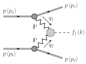
Figure 1: The Born-level diagram for the $\mathbb{P}\mathbb{P}$-fusion mechanism for central exclusive diffractive production of an $f_{1}$-type meson in proton-proton collisions.

The kinematic variables for the reaction (1) are

$$q_{1}=p_{a}-p_{1},\quad q_{2}=p_{b}-p_{2},\quad k=q_{1}+q_{2},$$

$$t_{1}=q_{1}^{2},\quad t_{2}=q_{2}^{2},\quad m_{f_{1}}^{2}=k^{2},$$

$$s=(p_{a}+p_{b})^{2}=(p_{1}+p_{2}+k)^{2},$$

$$s_{1}=(p_{a}+q_{2})^{2}=(p_{1}+k)^{2},$$

$$s_{2}=(p_{b}+q_{1})^{2}=(p_{2}+k)^{2}\,.$$ (2)

For the kinematics see e.g. Appendix D of Lebiedowicz:2013ika .

The amplitude for the reaction (1) can be written as

$${\cal M}_{\lambda_{a}\lambda_{b}\to\lambda_{1}\lambda_{2}\lambda}=(\epsilon_{\mu}(\lambda))^{*}\,{\cal M}^{\mu}_{\lambda_{a}\lambda_{b}\to\lambda_{1}\lambda_{2}f_{1}}\,,$$ (3)

where $\epsilon_{\mu}(\lambda)$ is the polarisation vector of the $f_{1}$ meson.

The Born-level $\mathbb{P}\mathbb{P}$-fusion amplitude for exclusive production of an axial-vector meson $f_{1}$ can be written as

$${\cal M}^{(\mathbb{P}\mathbb{P}\to f_{1})}_{\mu,\,\lambda_{a}\lambda_{b}\to\lambda_{1}\lambda_{2}f_{1}} = (-i)\,\bar{u}(p_{1},\lambda_{1})i\Gamma^{(\mathbb{P}pp)}_{\mu_{1}\nu_{1}}(p_{1},p_{a})u(p_{a},\lambda_{a})$$ (4)

$$\times i\Delta^{(\mathbb{P})\,\mu_{1}\nu_{1},\alpha_{1}\beta_{1}}(s_{1},t_{1})\,i\Gamma^{(\mathbb{P}\mathbb{P}f_{1})}_{\alpha_{1}\beta_{1},\alpha_{2}\beta_{2},\mu}(q_{1},q_{2})\,i\Delta^{(\mathbb{P})\,\alpha_{2}\beta_{2},\mu_{2}\nu_{2}}(s_{2},t_{2})$$

$$\times\bar{u}(p_{2},\lambda_{2})i\Gamma^{(\mathbb{P}pp)}_{\mu_{2}\nu_{2}}(p_{2},p_{b})u(p_{b},\lambda_{b})\,.$$

Here $\Delta^{(\mathbb{P})}$ and $\Gamma^{(\mathbb{P}pp)}$ denote the effective propagator and proton vertex function, respectively, for the tensor-pomeron exchange. The corresponding expressions, given in Sec. 3 of Ewerz:2013kda , are

$$i\Delta^{(\mathbb{P})}_{\mu\nu,\kappa\lambda}(s,t)=\frac{1}{4s}\left(g_{\mu\kappa}g_{\nu\lambda}+g_{\mu\lambda}g_{\nu\kappa}-\frac{1}{2}g_{\mu\nu}g_{\kappa\lambda}\right)(-is\alpha^{\prime}_{\mathbb{P}})^{\alpha_{\mathbb{P}}(t)-1}\,,$$ (5)

$$i\Gamma_{\mu\nu}^{(\mathbb{P}pp)}(p^{\prime},p)=-i3\beta_{\mathbb{P}NN}F_{1}(t)\left\{\frac{1}{2}\left[\gamma_{\mu}(p^{\prime}+p)_{\nu}+\gamma_{\nu}(p^{\prime}+p)_{\mu}\right]-\frac{1}{4}g_{\mu\nu}(\not\!p^{\prime}+\not\!p)\right\},\qquad$$ (6)

where $t=(p^{\prime}-p)^{2}$ and $\beta_{\mathbb{P}NN}=1.87$ GeV^-1. For simplicity we use for the pomeron-proton coupling the electromagnetic Dirac form factor $F_{1}(t)$ of the proton; see also Chapter 3.2 of Donnachie:2002en . The pomeron trajectory $\alpha_{\mathbb{P}}(t)$ is assumed to be of standard linear form (see, e.g., Donnachie:1992ny ; Donnachie:2002en ),

$$\alpha_{\mathbb{P}}(t)=\alpha_{\mathbb{P}}(0)+\alpha^{\prime}_{\mathbb{P}}\,t\,,$$ (7)

$$\alpha_{\mathbb{P}}(0)=1.0808\,,\;\;\alpha^{\prime}_{\mathbb{P}}=0.25\;\mathrm{GeV}^{-2}\,.$$ (8)

The new and unknown main ingredient of the amplitude (4) is the pomeron-pomeron-$f_{1}$ vertex $\Gamma^{(\mathbb{P}\mathbb{P}f_{1})}$ which we want to study in the present article. In Lebiedowicz:2013ika ; Lebiedowicz:2016ioh ; Lebiedowicz:2018eui ; Lebiedowicz:2016zka ; Lebiedowicz:2018sdt ; Lebiedowicz:2019jru ; Lebiedowicz:2019por the following strategy for constructing pomeron-pomeron-meson ($\mathbb{P}\mathbb{P}M$) couplings was followed. First, one looked at the possible couplings of two fictitious “real” pomerons to the meson $M$. This was easily done using elementary angular-momentum algebra; see Appendix A of Lebiedowicz:2013ika . Then $\mathbb{P}\mathbb{P}M$ couplings were written down corresponding to the allowed values of orbital angular momentum $l$ and total $\mathbb{P}\mathbb{P}$ spin $S$ for a given meson $M$ in question. Finally these couplings were also used for the CEP reaction $pp\to pMp$. We follow this strategy also for CEP of an $f_{1}$ meson. Thus, we investigate first the fictitious reaction

$$\mathbb{P}(t,\epsilon^{(1)})+\mathbb{P}(t,\epsilon^{(2)})\to f_{1}(k,\epsilon)\,,$$ (9)

where $\mathbb{P}$ are “real pomerons” of mass squared $t>0$ and with polarisation tensors $\epsilon^{(1)}$ and $\epsilon^{(2)}$.

From the analysis of this type of reactions presented in Appendix A of Lebiedowicz:2013ika we find that for the $f_{1}$ with $J^{P}=1^{+}$ there are two independent amplitudes for the reaction (9), labelled by $(l,S)=(2,2)$ and $(4,4)$. Convenient covariant couplings leading to these amplitudes are easily constructed; see (52) and (54) in Appendix A. But these constructions are not unique. In the Sakai-Sugimoto model Sakai:2004cn ; Sakai:2005yt the coupling of an $I^{G}=0^{+}$, $J^{P}=1^{+}$ axial-vector meson to two tensor glueballs is determined by the gravitational Chern-Simons (CS) action describing axial-gravitational anomalies; see (59) of Anderson:2014jia . Identifying the tensor glueballs with the fictitious “real pomerons” of (9) we have derived corresponding bare coupling Lagrangians $\mathbb{P}\mathbb{P}f_{1}$ in (61) and (62) of Appendix B.

For the fictitious on-shell process (9) the sum of the Lagrangians of (52) and (54) is strictly equivalent to the sum of (61) and (62). The relation of the respective coupling constants is given in (71). But for the realistic case where the pomerons have invariant masses $t_{1,2}<0$ and in general $t_{1}\neq t_{2}$ this equivalence no longer holds. But we can expect that for small values $|t_{1}|,|t_{2}|\lesssim 0.5$ GeV² the off-shell effects should not be drastic. And this, indeed, is confirmed by the explicit study presented in Appendix B.

In the following we shall present the formulas using the couplings (52) and (54) of Appendix A. The formulas using the couplings (61) and (62) of Appendix B are completely analogues. Results will be shown for both types of couplings.

From the coupling Lagrangians of Appendix A we obtain the following $\mathbb{P}\mathbb{P}f_{1}$ vertex:

$$i\Gamma_{\kappa\lambda,\rho\sigma,\alpha}^{(\mathbb{P}\mathbb{P}f_{1})}(q_{1},q_{2})=\left(i\Gamma_{\kappa\lambda,\rho\sigma,\alpha}^{\prime(\mathbb{P}\mathbb{P}f_{1})}(q_{1},q_{2})\mid_{\rm{bare}}+i\Gamma_{\kappa\lambda,\rho\sigma,\alpha}^{\prime\prime(\mathbb{P}\mathbb{P}f_{1})}(q_{1},q_{2})\mid_{\rm{bare}}\right)\tilde{F}_{\mathbb{P}\mathbb{P}f_{1}}(q_{1}^{2},q_{2}^{2},k^{2})\,.\qquad$$ (10)

The $\Gamma^{\prime}$ and $\Gamma^{\prime\prime}$ vertices in (10) correspond to $(l,S)=(2,2)$ and $(4,4)$, respectively, as derived from the corresponding coupling Lagrangians (52) and (54) in Appendix A. The expressions for these $\mathbb{P}\mathbb{P}f_{1}$ vertices  are as follows:
      

$$i\Gamma_{\kappa\lambda,\rho\sigma,\alpha}^{\prime(\mathbb{P}\mathbb{P}f_{1})}(q_{1},q_{2})\mid_{\rm{bare}}=-\frac{g^{\prime}_{\mathbb{P}\mathbb{P}f_{1}}}{8\,M_{0}^{2}}(q_{1}-q_{2})^{\mu}(q_{1}-q_{2})^{\nu}k^{\beta}\,\Gamma_{\kappa\lambda,\rho\sigma,\mu\nu,\alpha\beta}^{(8)}\,,$$ (11)

$$i\Gamma_{\kappa\lambda,\rho\sigma,\alpha}^{\prime\prime(\mathbb{P}\mathbb{P}f_{1})}(q_{1},q_{2})\mid_{\rm{bare}}=\frac{g^{\prime\prime}_{\mathbb{P}\mathbb{P}f_{1}}}{4\,M_{0}^{4}}(q_{1}-q_{2})^{\mu_{1}}(q_{1}-q_{2})^{\mu_{2}}(q_{1}-q_{2})^{\mu_{3}}(q_{1}-q_{2})^{\mu_{4}}k^{\beta}$$

$$\qquad\qquad\times\Bigl{[}(g_{\kappa\mu_{1}}g_{\lambda\mu_{2}}-\frac{1}{4}g_{\kappa\lambda}g_{\mu_{1}\mu_{2}})(g_{\rho\mu_{3}}\varepsilon_{\sigma\mu_{4}\alpha\beta}+g_{\sigma\mu_{3}}\varepsilon_{\rho\mu_{4}\alpha\beta})+(\kappa,\lambda)\leftrightarrow(\rho,\sigma)\Bigr{]}.\qquad$$ (12)

In (11) and (12) $M_{0}\equiv 1$ GeV, $k=q_{1}+q_{2}$, $\Gamma^{(8)}$ is defined in (49), and $g^{\prime}_{\mathbb{P}\mathbb{P}f_{1}}$, $g^{\prime\prime}_{\mathbb{P}\mathbb{P}f_{1}}$ are dimensionless coupling constants. The values of these coupling constants are not known and are not easy to obtain from first principles of QCD, as they are of nonperturbative origin. At the present stage the coupling constants $g_{\mathbb{P}\mathbb{P}f_{1}}^{\prime}$ and $g_{\mathbb{P}\mathbb{P}f_{1}}^{\prime\prime}$ should be fitted to experimental data.

For realistic applications we should multiply the “bare” vertices (11) and (12) by a form factor $\tilde{F}^{(\mathbb{P}\mathbb{P}f_{1})}$ which we take in the factorised ansatz as 

$$\tilde{F}^{(\mathbb{P}\mathbb{P}f_{1})}(q_{1}^{2},q_{2}^{2},k^{2})=F_{M}(q_{1}^{2})F_{M}(q_{2}^{2})F^{(\mathbb{P}\mathbb{P}f_{1})}(k^{2})\,.$$ (13)

For the on-shell meson we have $F^{(\mathbb{P}\mathbb{P}f_{1})}(m_{f_{1}}^{2})=1$. In (13) we use

$$F_{M}(t)=\frac{1}{1-t/\Lambda_{0}^{2}}\,,$$ (14)

with $\Lambda_{0}^{2}=0.5$ GeV²; see (3.34) of Ewerz:2013kda and (3.22) in Chapter 3.2 of Donnachie:2002en . Alternatively, we use the exponential form given as

$$\tilde{F}^{(\mathbb{P}\mathbb{P}f_{1})}(t_{1},t_{2},m_{f_{1}}^{2})=\exp\left(\frac{t_{1}+t_{2}}{\Lambda_{E}^{2}}\right)\,,$$ (15)

where we have set $k^{2}=m_{f_{1}}^{2}$ and the cutoff constant $\Lambda_{E}$ should be adjusted to experimental data.

In the high-energy and small-angle approximation, using (D.18) in Appendix D of Lebiedowicz:2013ika , the $\mathbb{P}\mathbb{P}$-fusion amplitude reads

$${\cal M}^{(\mathbb{P}\mathbb{P}\to f_{1})}_{\mu,\,\lambda_{a}\lambda_{b}\to\lambda_{1}\lambda_{2}f_{1}} = i\,3\beta_{\mathbb{P}NN}\,F_{1}(t_{1})\,(p_{1}+p_{a})^{\alpha_{1}}(p_{1}+p_{a})^{\beta_{1}}\,\delta_{\lambda_{1}\lambda_{a}}$$ (16)

$$\times\frac{1}{2s_{1}}\left(-is_{1}\alpha^{\prime}_{\mathbb{P}}\right)^{\alpha_{\mathbb{P}}(t_{1})-1}i\Gamma^{(\mathbb{P}\mathbb{P}f_{1})}_{\alpha_{1}\beta_{1},\alpha_{2}\beta_{2},\mu}(q_{1},q_{2})\,\frac{1}{2s_{2}}\left(-is_{2}\alpha^{\prime}_{\mathbb{P}}\right)^{\alpha_{\mathbb{P}}(t_{2})-1}$$

$$\times 3\beta_{\mathbb{P}NN}\,F_{1}(t_{2})\,(p_{2}+p_{b})^{\alpha_{2}}(p_{2}+p_{b})^{\beta_{2}}\,\delta_{\lambda_{2}\lambda_{b}}\,.$$

For the $\mathbb{P}\mathbb{P}f_{1}$ vertex function we shall use in the following the form (10) with the bare vertices either from (11) and (12) (corresponding to the couplings discussed in Appendix A) or those from (66) and (67) from Appendix B.

Note that the vertices (11) and (12) derived from the coupling Lagrangians (52) and (54) automatically are divergence free; i.e., they satisfy

$$i\Gamma^{(\mathbb{P}\mathbb{P}f_{1})}_{\kappa\lambda,\rho\sigma,\alpha}(q_{1},q_{2})\,(q_{1}+q_{2})^{\alpha}=0\,.$$ (17)

For the vertices derived from (61) and (62) this does not hold. Thus, in calculations of cross sections with the vertices (66) and (67) one has to use for the $f_{1}$ spin sum

$$-g_{\mu\nu}+\frac{k_{\mu}k_{\nu}}{k^{2}}\,,$$ (18)

since the $k_{\mu}k_{\nu}$ term will give a nonzero contribution. With the vertices from (11) and (12) the $k_{\mu}k_{\nu}$ term does not contribute.

To give the full amplitude for the reaction (1) we should also include absorption effects to the Born amplitude:

$${\cal{M}}_{pp\to ppf_{1}}={\cal{M}}_{pp\to ppf_{1}}^{\rm Born}+{\cal{M}}_{pp\to ppf_{1}}^{pp-\rm{rescattering}}\,.$$ (19)

In our analysis we include the absorptive corrections within the one-channel-eikonal approach. For investigations of an eikonal model see, e.g., Gotsman:1998mm . The main result of Gotsman:1998mm is that the absorption effects become more important at higher energies; that is, the survival probability of large rapidity gaps decreases with increasing energy. A two-channel eikonal model was discussed in Khoze:2000wk ; Khoze:2002nf ; Khoze:2013dha . A more sophisticated three-channel model was discussed in Gotsman:1999xq .

The amplitude including the “soft” $pp$-rescattering corrections which we use in the present paper can be written as

$${\cal M}_{pp\to ppf_{1}}^{pp-\rm{rescattering}}(s,\mbox{\boldmath$p_{t,1}$},\mbox{\boldmath$p_{t,2}$})=\frac{i}{8\pi^{2}s}\int d^{2}\mbox{\boldmath$k_{t}$}\,{\cal M}_{pp\to pp}(s,-\mbox{\boldmath{$k_{t}^{2}$}}){\cal M}_{pp\to ppf_{1}}^{\rm Born}(s,\mbox{\boldmath$\tilde{p}_{t,1}$},\mbox{\boldmath$\tilde{p}_{t,2}$})\,.\qquad\;\;$$ (20)

Here, in the overall center-of-mass (c.m.) system, $p_{t,1}$ and $p_{t,2}$ are the transverse components of the momenta of the outgoing protons and $k_{t}$ is the transverse momentum carried around the pomeron loop. ${\cal M}_{pp\to ppf_{1}}^{\rm Born}$ is the Born amplitude given by (3) and (16) with $\mbox{\boldmath$\tilde{p}_{t,1}$}=\mbox{\boldmath$p_{t,1}$}-\mbox{\boldmath$k_{t}$}$ and $\mbox{\boldmath$\tilde{p}_{t,2}$}=\mbox{\boldmath$p_{t,2}$}+\mbox{\boldmath$k_{t}$}$. ${\cal M}_{pp\to pp}$ is the elastic $pp$ scattering amplitude given by (6.28) in Ewerz:2013kda for large $s$ and with the momentum transfer $t=-\mbox{\boldmath{$k_{t}^{2}$}}$. In practice we work with the amplitudes in the high-energy approximation, i.e. assuming $s$-channel helicity conservation as it is realized in our model.

III Results

In this section we wish to present first results for the $pp\to ppf_{1}(1285)$ and $pp\to ppf_{1}(1420)$ reactions. We will first discuss the $pp\to ppf_{1}$ reactions at the relatively low c.m. energy $\sqrt{s}=29.1$ GeV and compare our model results with the WA102 experimental data from Barberis:1998by . We shall try to fix the parameters of our model including at first only the $\mathbb{P}\mathbb{P}$-fusion mechanism. Then we shall make predictions for the experiments at the RHIC and LHC. The secondary reggeon exchanges should give small contributions at high energies and in the midrapidity region. However, they may influence the absolute normalization of the cross section at low energies. Therefore, our predictions for the RHIC and LHC experiments, obtained in this way, should be regarded rather as an upper limit for the $pp\to ppf_{1}$ reactions, but, as discussed in Appendix D, we expect that they should overestimate the cross sections by not more than a factor of 4.

III.1 Comparison with the WA102 data

According to Barberis:1998by the WA102 experimental cross sections are as quoted in Table 1.

Table 1: Experimental results for total cross sections of $f_{1}$ mesons in $pp$ collisions measured by the WA102 Collaboration Barberis:1998by .

Meson	$\sqrt{s}$ (GeV)	Cuts	$\sigma_{\rm{exp.}}$ (nb)
$f_{1}(1285)$	12.7	$|x_{F,M}|\leqslant 0.2$	$6857\pm 1306$
	29.1	$|x_{F,M}|\leqslant 0.2$	$6919\pm 886$
$f_{1}(1420)$	12.7	$|x_{F,M}|\leqslant 0.2$	$1080\pm 385$
	29.1	$|x_{F,M}|\leqslant 0.2$	$1584\pm 145$

In Barberis:1998by  also the distributions in $|t|$ and $\phi_{pp}$ for the $f_{1}(1285)$ and $f_{1}(1420)$ meson production at $\sqrt{s}=29.1$ GeV were presented. Here, $t$ is the four-momentum transfer squared from one of the proton vertices [we have $t=t_{1}$ or $t_{2}$; cf. (2)], and $\phi_{pp}$ is the azimuthal angle between the transverse momentum vectors $p_{t,1}$ and $p_{t,2}$ of the outgoing protons (see Fig. 12 in Appendix E).

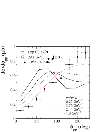
Figure 7: The $\phi_{pp}$ distributions for the $pp\to ppf_{1}(1420)$ reaction at $\sqrt{s}=29.1$ GeV and $|x_{F,M}|\leqslant 0.2$. The theoretical results and the WA102 data points from Barberis:1998by have been normalised to the mean value of the total cross section (33). The meaning of the lines is as in Fig. 5.

Below we present three independent ways to fix the $\mathbb{P}\mathbb{P}f_{1}$ coupling parameters in the $pp\to ppf_{1}(1285)$ reaction. First we assume that only one of the couplings $g^{\prime}_{\mathbb{P}\mathbb{P}f_{1}}$ or $g^{\prime\prime}_{\mathbb{P}\mathbb{P}f_{1}}$ [$(l,S)=(2,2)$ term (11) or $(l,S)=(4,4)$ term (12)] contributes, and we make evaluations and comparisons with the WA102 experimental data; see Figs. 2, 3 and Table 2. Later we consider the combination of two terms, the $\varkappa^{\prime}$ and $\varkappa^{\prime\prime}$ couplings calculated with the vertices (66) and (67); see Fig. 5. We will also show to which values of $g^{\prime}_{\mathbb{P}\mathbb{P}f_{1}}$ and $g^{\prime\prime}_{\mathbb{P}\mathbb{P}f_{1}}$ the $(\varkappa^{\prime},\varkappa^{\prime\prime})$ values correspond. Then we follow the analogous procedure to fix the $\mathbb{P}\mathbb{P}f_{1}(1420)$ couplings; see Figs. 6, 7 and Table 2.

In Fig. 2 we show the results for the $f_{1}(1285)$ meson production for $\sqrt{s}=29.1$ GeV and for the Feynman variable of the meson $|x_{F,M}|\leqslant 0.2$. The WA102 data points from Barberis:1998by and our model results have been normalised to the mean value of the total cross section

$$\sigma_{\rm exp.}=(6919\pm 886)\;\mathrm{nb}\,;$$ (21)

see Table 1. The experimental error of the total cross section is about 12.8 % (21) and is dominated by systematic effects. Correspondingly the error bars quoted in Fig. 2 are assumed to be 12.8 % of the cross section for each bin.

We show the results for different $\mathbb{P}\mathbb{P}f_{1}$ couplings discussed in the present paper. The theoretical calculations in the top panels of Fig. 2 correspond to the $(l,S)=(2,2)$ term (11) while those in the bottom panels to the $(4,4)$ term (12). We can see from the left panels of Fig. 2 that the $t$ dependence of $f_{1}$ production is very sensitive to the form factor $\tilde{F}^{(\mathbb{P}\mathbb{P}f_{1})}$ in the pomeron-pomeron-meson vertex. The results with the exponential form (15) and $\Lambda_{E}=0.7$ GeV describe the $t$ dependence better than (13) with (14). The calculations with (15) give a sizeable decrease of the cross section at large $|t|$. Therefore, in the following we show the results calculated with (15). At $t=0$ (here $t=t_{1}$ or $t_{2}$) all contributions vanish. Both the $(l,S)=(2,2)$ and $(4,4)$ couplings considered separately allow one to describe the WA102 differential distributions.

To get the mean value of the total cross section (21) we find the following: $g^{\prime}_{\mathbb{P}\mathbb{P}f_{1}}=4.89$ in (11) for $\Lambda_{E}=0.7$ GeV, $g^{\prime}_{\mathbb{P}\mathbb{P}f_{1}}=6.00$ for $\Lambda_{E}=0.6$ GeV, $g^{\prime\prime}_{\mathbb{P}\mathbb{P}f_{1}}=10.31$ in (12) for $\Lambda_{E}=0.7$ GeV, $g^{\prime\prime}_{\mathbb{P}\mathbb{P}f_{1}}=12.90$ for $\Lambda_{E}=0.6$ GeV, $\varkappa^{\prime}=8.58$ in (66) for $\Lambda_{E}=0.7$ GeV, and $\varkappa^{\prime}=7.40$ for $\Lambda_{E}=0.8$ GeV. Here we assumed the value of coupling constants to be positive as we employ them separately.

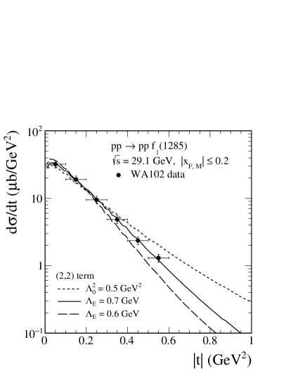
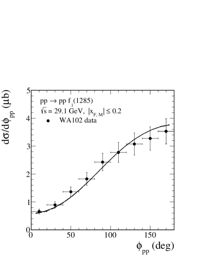
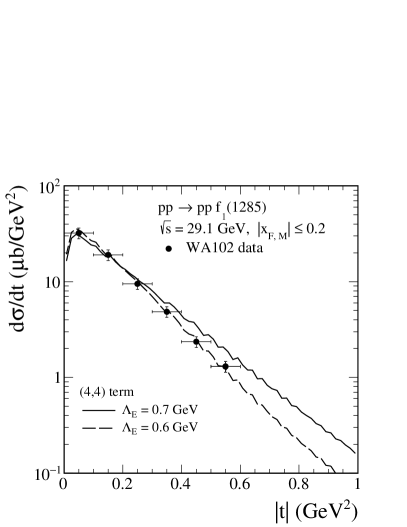
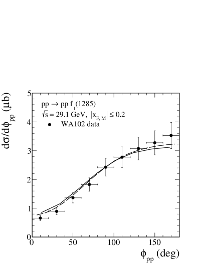
Figure 2: The $|t|$ (left panels) and $\phi_{pp}$ (right panels) distributions for the $pp\to ppf_{1}(1285)$ reaction at $\sqrt{s}=29.1$ GeV and $|x_{F,M}|\leqslant 0.2$. The results have been normalised to the mean value of the total cross section (21) from Barberis:1998by . The error bars on the data correspond to the error on $\sigma_{\rm exp.}$ in (21). The separate individual contributions for the $(l,S)=(2,2)$ [see Eq. (11)] (upper panels) and $(l,S)=(4,4)$ [see Eq. (12)] (lower panels) are presented. We show results obtained with the exponential form factor (15) for $\Lambda_{E}=0.7$ GeV (solid lines) and for $\Lambda_{E}=0.6$ GeV (long-dashed lines). The dotted line in the top left panel is obtained using (13) with (14). The absorption effects are included in the calculations. The oscillations in the left bottom panel are of numerical origin.

In Kirk:1999df an interesting behaviour of the $\phi_{pp}$ distribution for $f_{1}(1285)$ meson production for two different values of $|t_{1}-t_{2}|$ was presented. In Fig. 3 we show the $\phi_{pp}$ distribution of events from Kirk:1999df for $|t_{1}-t_{2}|\leqslant 0.2$ GeV² (left panel) and $|t_{1}-t_{2}|\geqslant 0.4$ GeV² (right panel). Our model results have been normalised to the mean value of the number of events. The results for $\Lambda_{E}=0.7$ GeV in (15) are shown. We have checked that for $\Lambda_{E}=0.6$ GeV the shape of the $\phi_{pp}$ distributions is almost the same. An almost “flat” distribution at large values of $|t_{1}-t_{2}|$ can be observed. It seems that the $(l,S)=(4,4)$ term best reproduces the shape of the WA102 data. As we will show below in Fig. 4, the absorption effects play a significant role there.

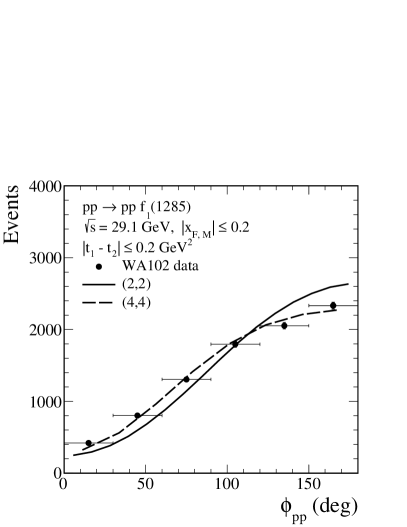
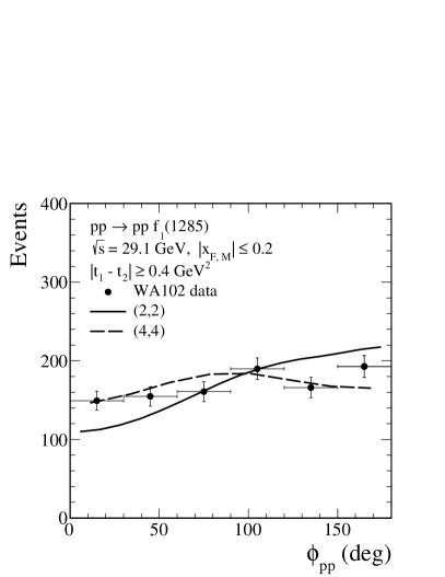
Figure 3: The $\phi_{pp}$ distributions for $f_{1}(1285)$ meson production at $\sqrt{s}=29.1$ GeV, $|x_{F,M}|\leqslant 0.2$, and for $|t_{1}-t_{2}|\leqslant 0.2$ GeV² (left panel) and $|t_{1}-t_{2}|\geqslant 0.4$ GeV² (right panel). The WA102 experimental data points are from Fig. 3 of Kirk:1999df . The theoretical results have been normalised to the mean value of the number of events. In the calculation we use here (15) with $\Lambda_{E}=0.7$ GeV. The absorption effects are included here.

Note that in Kirk:1999df also the number of events for the $f_{1}(1285)$ meson for the two kinematical conditions (a) $|t_{1}-t_{2}|\leqslant 0.2$ GeV² and (b) $|t_{1}-t_{2}|\geqslant 0.4$ GeV² was given. The experimental ratio is $R_{\rm exp.}=N_{a}/N_{b}\simeq 8.6$, where $N_{a}$ and $N_{b}$ are the number of events from Figs. 3(a) and 3(b) of Kirk:1999df , respectively. Then, we define the ratio

$$R=\frac{\sigma(|t_{1}-t_{2}|\leqslant 0.2\;{\rm GeV}^{2})}{\sigma(|t_{1}-t_{2}|\geqslant 0.4\;{\rm GeV}^{2})}\,.$$ (22)

From our model using $\Lambda_{E}=0.7$ GeV in (15) we get for the $(2,2)$ term (11) the ratio $R=8.6$, while for the $(4,4)$ term (12) we get $R=5.6$. If we use $\Lambda_{E}=0.6$ GeV we get $R=15.9$ and $R=10.3$, respectively. Therefore, for the $(2,2)$ term, $\Lambda_{E}=0.7$ GeV is a good choice, while for the $(4,4)$ term we should use a bit smaller value. For the $\varkappa^{\prime}$ term given by (66) and $\Lambda_{E}=0.7$ GeV we get $R=13.2$ while for $\Lambda_{E}=0.8$ GeV we get $R=8.8$. For the $(\varkappa^{\prime},\varkappa^{\prime\prime})$ terms, respectively for $\varkappa^{\prime\prime}/\varkappa^{\prime}=-(6.25,3.76,2.44,1.0)\;\mathrm{GeV}^{-2}$ and $\Lambda_{E}=0.7$ GeV we get $R=(7.6,10.5,11.9,13.2)$.

In Fig. 4 we show the results for the $\phi_{pp}$ distributions for different cuts on $|t_{1}-t_{2}|$ without and with the absorption effects included in the calculations. The results for the two $(l,S)$ couplings are shown. The absorption effects lead to a large reduction of the cross section. We obtain the ratio of full and Born cross sections, the survival factor, as $\langle S^{2}\rangle=0.5$–$0.7$. Note that $\langle S^{2}\rangle$ depends on the kinematics. We can see a large damping of the cross section in the region of $\phi_{pp}\sim\pi$, especially for $|t_{1}-t_{2}|\geqslant 0.4$ GeV². We notice that our results for the $(4,4)$ term have similar shapes as those presented in Petrov:2004hh [see Figs. 3(c) and 3(d)] where the authors also included the absorption corrections.

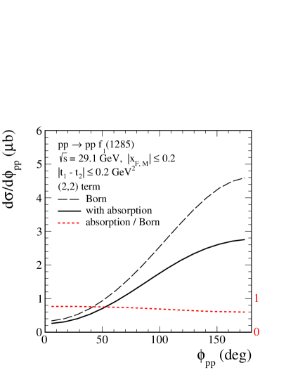
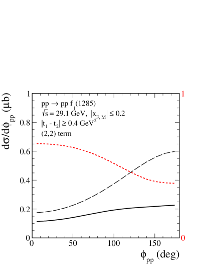
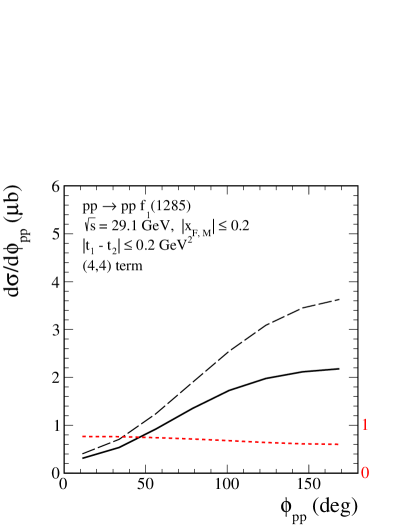
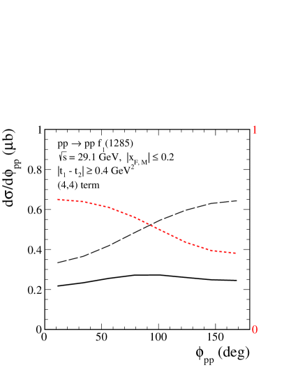
Figure 4: The $\phi_{pp}$ distributions for $f_{1}(1285)$ meson production at $\sqrt{s}=29.1$ GeV, $|x_{F,M}|\leqslant 0.2$, and for $|t_{1}-t_{2}|\leqslant 0.2$ GeV² (left panels) and for $|t_{1}-t_{2}|\geqslant 0.4$ GeV² (right panels). In the calculation here we use (15) with $\Lambda_{E}=0.7$ GeV. The top panels show the results for the $(l,S)=(2,2)$ term and $g^{\prime}_{\mathbb{P}\mathbb{P}f_{1}}=4.89$ [see Eq. (11)] and the bottom panels show the $(l,S)=(4,4)$ term and $g^{\prime\prime}_{\mathbb{P}\mathbb{P}f_{1}}=10.31$ [see Eq. (12)]. The long-dashed black lines represent the Born results and the solid black lines correspond to the results with the absorption effects included. The dotted red lines represent the ratio of full and Born cross sections on the scale indicated by the red numbers on the right-hand side of the panels.

In Barberis:1998by also the ${\rm dP_{t}}$ dependence for both the $f_{1}(1285)$ and the $f_{1}(1420)$ mesons was presented. Here, ${\rm dP_{t}}$ (the so-called “glueball-filter variable” Close:1997pj ; Barberis:1996iq ) is defined as

$$\mbox{\boldmath$dP_{t}$}=\mbox{\boldmath$q_{t,1}$}-\mbox{\boldmath$q_{t,2}$}=\mbox{\boldmath$p_{t,2}$}-\mbox{\boldmath$p_{t,1}$}\,,\quad{\rm dP_{t}}=|\mbox{\boldmath$dP_{t}$}|\,.$$ (23)

The experimental values for the cross sections in three ${\rm dP_{t}}$ intervals and for the ratio of $f_{1}$ production at small ${\rm dP_{t}}$ to large ${\rm dP_{t}}$ are given there. In Table 2 we show the WA102 data and our corresponding results for the different $\mathbb{P}\mathbb{P}f_{1}$ couplings. The small values of the experimental ratios for the $f_{1}(1285)$ and the $f_{1}(1420)$ as listed in the last column may signal that these two mesons are predominantly $q\bar{q}$ states Close:1997pj . From the comparison of the first four rows we see again that the exponential form of the $t$ dependences in the $(l,S)=(2,2)$ $\mathbb{P}\mathbb{P}f_{1}(1285)$ vertex is preferred. For the $(4,4)$ term an optimal value of the $\Lambda_{E}$ parameter is in the range of (0.6–0.7) GeV. There are also shown the results obtained for the couplings (66) and (67) and for the ratio of coupling constants from (24); see (65) of Appendix B. For comparison, the results for $\varkappa^{\prime\prime}/\varkappa^{\prime}=-1.0$ GeV^-2 are also presented. We use here the form factor (15) with $\Lambda_{E}=0.7$ GeV.

Table 2: Results of $f_{1}$-meson production as a function of ${\rm dP_{t}}$ (23), in three ${\rm dP_{t}}$ intervals, expressed as a percentage of the total contribution at the WA102 collision energy $\sqrt{s}=29.1$ GeV and for $|x_{F,M}|\leqslant 0.2$. In the last column the ratios of $\sigma({\rm dP_{t}}\leqslant\,0.2~{}\mathrm{GeV})/\sigma({\rm dP_{t}}\geqslant\,0.5~{}\mathrm{GeV})$ are given. The experimental numbers are from Barberis:1998by . The theoretical numbers correspond to the separate individual coupling terms $(l,S)=(2,2)$ and $(4,4)$ [see (11) and (12), respectively] for different $\Lambda_{E}$ parameters in the relevant type of the $\mathbb{P}\mathbb{P}f_{1}$ form factor. The $\varkappa^{\prime}$ and $\varkappa^{\prime\prime}$ results were calculated from (66) and (67), respectively. We show the results for the coupling range given by Eq. (24) and the result for $\varkappa^{\prime\prime}/\varkappa^{\prime}=-1.0$ GeV^-2 from our fit to the WA102 data. The absorption effects have been included in our analysis within the one-channel-eikonal approach.

Meson		${\rm dP_{t}}\leqslant 0.2$ GeV	$0.2\leqslant{\rm dP_{t}}\leqslant 0.5$ GeV	${\rm dP_{t}}\geqslant 0.5$ GeV	Ratio
$f_{1}(1285)$	Experiment Barberis:1998by	$3\pm 1$	$35\pm 2$	$61\pm 4$	$0.05\pm 0.02$
	$(2,2)$, $\Lambda_{0}^{2}=0.5$ GeV2	1.5	30.3	68.1	0.02
	$(2,2)$, $\Lambda_{E}=0.6$ GeV	2.6	43.9	53.5	0.05
	$(2,2)$, $\Lambda_{E}=0.7$ GeV	2.0	37.1	60.9	0.03
	$(4,4)$, $\Lambda_{E}=0.6$ GeV	2.5	43.7	53.7	0.05
	$(4,4)$, $\Lambda_{E}=0.7$ GeV	1.9	36.8	61.3	0.03
	$\varkappa^{\prime}$, $\Lambda_{E}=0.7$ GeV	2.0	37.5	60.5	0.03
	$\varkappa^{\prime}$, $\Lambda_{E}=0.8$ GeV	1.7	32.5	65.8	0.03
	$(\varkappa^{\prime},\varkappa^{\prime\prime})$, $\Lambda_{E}=0.7$ GeV:
	$\varkappa^{\prime\prime}/\varkappa^{\prime}=-6.25$ GeV-2	3.7	55.9	40.4	0.09
	$\varkappa^{\prime\prime}/\varkappa^{\prime}=-3.76$ GeV-2	3.2	54.1	42.7	0.08
	$\varkappa^{\prime\prime}/\varkappa^{\prime}=-2.44$ GeV-2	2.8	50.1	47.1	0.06
	$\varkappa^{\prime\prime}/\varkappa^{\prime}=-1.0$ GeV-2	2.4	41.8	55.8	0.04
$f_{1}(1420)$	Experiment Barberis:1998by	$2\pm 2$	$38\pm 2$	$60\pm 4$	$0.03\pm 0.03$
	$(2,2)$, $\Lambda_{0}^{2}=0.5$ GeV2	1.6	30.7	67.7	0.02
	$(2,2)$, $\Lambda_{E}=0.6$ GeV	2.7	44.3	53.0	0.05
	$(2,2)$, $\Lambda_{E}=0.7$ GeV	2.0	37.5	60.5	0.03
	$(2,2)$, $\Lambda_{E}=0.8$ GeV	1.6	32.7	65.7	0.02
	$(4,4)$, $\Lambda_{E}=0.6$ GeV	2.6	44.0	53.4	0.05
	$(4,4)$, $\Lambda_{E}=0.7$ GeV	2.0	37.1	60.9	0.03
	$\varkappa^{\prime}$, $\Lambda_{E}=0.7$ GeV	2.0	37.8	60.2	0.03
	$\varkappa^{\prime}$, $\Lambda_{E}=0.8$ GeV	1.7	33.0	65.3	0.03
	$(\varkappa^{\prime},\varkappa^{\prime\prime})$, $\Lambda_{E}=0.7$ GeV:
	$\varkappa^{\prime\prime}/\varkappa^{\prime}=-6.25$ GeV-2	3.7	56.2	40.1	0.09
	$\varkappa^{\prime\prime}/\varkappa^{\prime}=-3.76$ GeV-2	3.3	54.2	42.5	0.08
	$\varkappa^{\prime\prime}/\varkappa^{\prime}=-2.44$ GeV-2	2.9	50.3	47.8	0.06
	$\varkappa^{\prime\prime}/\varkappa^{\prime}=-1.0$ GeV-2	2.4	44.4	53.2	0.04

Up to now, in Figs. 2, 3 and 4, we have shown the contributions of the individual $(l,S)$ terms (couplings), calculated with the vertices (11) and (12), separately.

In Fig. 5 we examine the combination of two $\mathbb{P}\mathbb{P}f_{1}$ couplings $\varkappa^{\prime}$ and $\varkappa^{\prime\prime}$ calculated with the vertices (66) and (67), respectively. We can see that the best fit is for the ratio $\varkappa^{\prime\prime}/\varkappa^{\prime}\simeq-1.0$ GeV^-2 (see the red dotted lines on the top panels), which roughly agrees with the preliminary analysis performed in Hechenberger:thesis (cf. Eq. (2.68) in Hechenberger:thesis ).

As discussed in Appendix B, the prediction for $\varkappa^{\prime\prime}/\varkappa^{\prime}$ obtained in the Sakai-Sugimoto model is

$$\varkappa^{\prime\prime}/\varkappa^{\prime}=-(6.25\cdots 2.44)\;\mathrm{GeV}^{-2}$$ (24)

for $M_{\mathrm{KK}}=(949\cdots 1532)\;\mathrm{MeV}$. This agrees with the above fit ($\varkappa^{\prime\prime}/\varkappa^{\prime}=-1.0$ GeV^-2) as far as the sign of this ratio is concerned, but not in its magnitude. Other than a simple inadequacy of the Sakai-Sugimoto model, this could indicate that the Sakai-Sugimoto model needs a more complicated form of reggeization of the tensor glueball propagator as indeed discussed in Anderson:2014jia in the context of CEP of $\eta$ and $\eta^{\prime}$ mesons. It could also be an indication of the importance of secondary reggeon exchanges.

Fitting the mean value of the total cross section (21) we find

$$(\varkappa^{\prime},\varkappa^{\prime\prime})=\begin{cases}(-8.88,8.88\;{\rm GeV}^{-2})&\mbox{for}\;\varkappa^{\prime\prime}/\varkappa^{\prime}=-1.0~{}\mathrm{GeV}^{-2}\,,\\ (-9.14,22.30\;{\rm GeV}^{-2})&\phantom{\mbox{for}\;}\varkappa^{\prime\prime}/\varkappa^{\prime}=-2.44~{}\mathrm{GeV}^{-2}\,,\\ (-9.22,34.67\;{\rm GeV}^{-2})&\phantom{\mbox{for}\;}\varkappa^{\prime\prime}/\varkappa^{\prime}=-3.76~{}\mathrm{GeV}^{-2}\,,\\ (-8.81,55.06\;{\rm GeV}^{-2})&\phantom{\mbox{for}\;}\varkappa^{\prime\prime}/\varkappa^{\prime}=-6.25~{}\mathrm{GeV}^{-2}\,.\end{cases}$$ (25)

Taking into account the experimental errors (21) assumed to be 12.8 % of the cross section for each bin (see the bottom panels of Fig. 5), we get an error of our result for $\varkappa^{\prime\prime}/\varkappa^{\prime}=-1.0$ GeV^-2 of about 6 %. Thus the 1 standard deviation (s.d.) interval is here

$$(\varkappa^{\prime},\varkappa^{\prime\prime})=(-8.35,\;8.35\;{\rm GeV}^{-2})\cdots(-9.41,\;9.41\;{\rm GeV}^{-2})\quad\mbox{for}\;\varkappa^{\prime\prime}/\varkappa^{\prime}=-1.0~{}\mathrm{GeV}^{-2}\,.$$ (26)

In the bottom right panel of Fig. 5 we show results for the total $\phi_{pp}$ distribution for the individual $\varkappa^{\prime}$ and $\varkappa^{\prime\prime}$ coupling terms and for their coherent sum. Here we take $(\varkappa^{\prime},\varkappa^{\prime\prime})=(-8.88,\;8.88\;{\rm GeV}^{-2})$. The interference effect of the $\varkappa^{\prime}$ and $\varkappa^{\prime\prime}$ terms is clearly seen there. As we see from (72) the $\varkappa^{\prime\prime}$ term corresponds (approximately) to a superposition of the $(l,S)=(2,2)$ and $(4,4)$ terms with opposite signs. We expect then destructive interference of the two $(l,S)$ terms, and indeed, the $\varkappa^{\prime\prime}$ contribution shows such a behaviour; i.e., there is a complete cancellation of the two $(l,S)$ terms for $\phi_{pp}\simeq 90^{\circ}$. Hence, the option $\varkappa^{\prime}=0$, $\varkappa^{\prime\prime}\neq 0$ is clearly ruled out by the data for the $\phi_{pp}$ distribution. In fact, this option is also incompatible with the result (65) obtained in the Sakai-Sugimoto model, since it would correspond to the limit $M_{\mathrm{KK}}\to 0$ where the holographic model ceases to have large-$N_{c}$ QCD as its infrared limit.

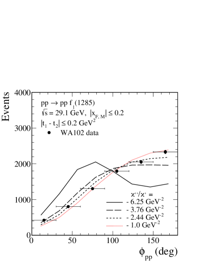
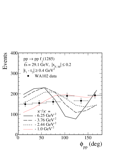
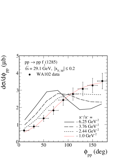
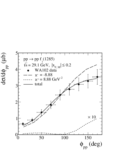
Figure 5: The $\phi_{pp}$ distributions for $f_{1}(1285)$ meson production at $\sqrt{s}=29.1$ GeV. Results for the $(\varkappa^{\prime},\varkappa^{\prime\prime})$ term calculated with the vertices (66) and (67) are shown. We use here the form factor (15) with $\Lambda_{E}=0.7$ GeV. In the top panels the theoretical results have been normalised to the mean value of the number of events from Kirk:1999df . In the bottom panels we compare the theoretical curves with the WA102 data from Barberis:1998by . Here the results have been normalised to the mean value of the total cross section (21) and the error bars on the data have been calculated as in Fig. 2. In the bottom right panel we show the results for $(\varkappa^{\prime},\varkappa^{\prime\prime})=(-8.88,\;8.88\;{\rm GeV}^{-2})$ for the individual $\varkappa^{\prime}$ and $\varkappa^{\prime\prime}$ coupling terms and for their coherent sum. The $\varkappa^{\prime\prime}$ contribution has been enhanced by a factor of 10 for better visibility. The absorption effects are included in the calculations.

Summarizing our findings for $f_{1}(1285)$ CEP, we have obtained a reasonable description of the WA102 data with either a pure $(l,S)=(2,2)$ or a pure $(l,S)=(4,4)$ coupling, as well as with the $\varkappa^{\prime},\varkappa^{\prime\prime}$ couplings with parameters,

$$(l,S)=(2,2)\;\mathrm{term}\mathrel{\mathop{\mathchar 58\relax}} \;\,g^{\prime}_{\mathbb{P}\mathbb{P}f_{1}}=4.89\,,\;g^{\prime\prime}_{\mathbb{P}\mathbb{P}f_{1}}=0\,,\;\Lambda_{E}=0.7\;\mathrm{GeV}\,;$$ (27)

$$(l,S)=(4,4)\;\mathrm{term}\mathrel{\mathop{\mathchar 58\relax}} \;\,g^{\prime}_{\mathbb{P}\mathbb{P}f_{1}}=0\,,\;g^{\prime\prime}_{\mathbb{P}\mathbb{P}f_{1}}=10.31\,,\;\Lambda_{E}=0.7\;\mathrm{GeV}\,;$$ (28)

$$\varkappa^{\prime}\;\mathrm{term\;only}\mathrel{\mathop{\mathchar 58\relax}} \;\,|\varkappa^{\prime}|=8.58\,,\;\varkappa^{\prime\prime}=0\,,\;\Lambda_{E}=0.7\;\mathrm{GeV}\,;$$ (29)

$$(\varkappa^{\prime},\varkappa^{\prime\prime})\;\mathrm{term}\mathrel{\mathop{\mathchar 58\relax}} \;\,\varkappa^{\prime}=-8.88\,,\;\varkappa^{\prime\prime}=8.88\;\mathrm{GeV}^{-2}\,,\;\Lambda_{E}=0.7\;\mathrm{GeV}\,.$$ (30)

As discussed in (26) the purely statistical errors on the coupling parameters (27)–(30) are estimated to be around 6 %.

It is also interesting to compare the results (27) and (29) with the approximate relation (72) for $\varkappa^{\prime\prime}=0$ and $k^{2}=m_{f_{1}}^{2}$. We note that we see no way to fix the overall sign of the $f_{1}$ couplings from experiment. The states $\ket{f_{1}}$ and $-\ket{f_{1}}$ are clearly equivalent from quantum mechanics. Of course, relative signs of couplings have physical significance, for instance, the relative sign of $g^{\prime}_{\mathbb{P}\mathbb{P}f_{1}}$ and $g^{\prime\prime}_{\mathbb{P}\mathbb{P}f_{1}}$. Keeping this in mind we compare the absolute values of the left-hand side (l.h.s.) and right-hand side (r.h.s.) of (72). With $m_{f_{1}}=(1281.9\pm 0.5)$ MeV Tanabashi:2018oca we get

$$\mathinner{\!\left\lvert\frac{g^{\prime}_{\mathbb{P}\mathbb{P}f_{1}}}{\varkappa^{\prime}}\right\rvert}=0.57\,,\quad\frac{M_{0}^{2}}{m_{f_{1}}^{2}}=0.61\,.$$ (31)

This shows that the approximate relation (72) is here satisfied to an accuracy of around 10 %.

Using (72) we can also see to which values of $g^{\prime}_{\mathbb{P}\mathbb{P}f_{1}}$ and $g^{\prime\prime}_{\mathbb{P}\mathbb{P}f_{1}}$ the $(\varkappa^{\prime},\varkappa^{\prime\prime})$ values of (30) roughly correspond. With (30) and setting $t_{1}=t_{2}=-0.1$ GeV² in (72) we get

$$g^{\prime}_{\mathbb{P}\mathbb{P}f_{1}}=0.42\,,\quad g^{\prime\prime}_{\mathbb{P}\mathbb{P}f_{1}}=10.81\,.$$ (32)

Thus, $(\varkappa^{\prime},\varkappa^{\prime\prime})$ from (30) corresponds practically to a pure $(l,S)=(4,4)$ term and the values for $g^{\prime\prime}_{\mathbb{P}\mathbb{P}f_{1}}$ from (28) and (32) agree to within 5 % accuracy.

Now we present a comparison of our theoretical results also for the $f_{1}(1420)$ meson with relevant data from the WA102 experiment Barberis:1998by . In Fig. 6 we show the $|t|$ (left panels) and $\phi_{pp}$ (right panels) distributions for $\sqrt{s}=29.1$ GeV and $|x_{F,M}|\leqslant 0.2$. The WA102 data points from Barberis:1998by and our model results have been normalised to the mean value of the total cross section

$$\sigma_{\rm exp.}=(1584\pm 145)\;\mathrm{nb}\,;$$ (33)

see Table 1. The experimental error bars are assumed to be 9.2 % corresponding to the error of $\sigma_{\rm exp.}$ in (33).

From Fig. 6 we can see that the $(l,S)=(2,2)$ term is sufficient to describe the WA102 data. We have checked that the shape of $\phi_{pp}$ distributions almost does not depend on the choice of the cutoff parameter $\Lambda_{E}$, in particular for the $(l,S)=(2,2)$ term. Taking into account the results listed in Table 2 we conclude that $\Lambda_{E}=0.7$ GeV is an optimal choice. To get the mean value of the total cross section (33) we find (assuming positive values of the coupling constants): $g^{\prime}_{\mathbb{P}\mathbb{P}f_{1}(1420)}=2.06$ in (11) for $\Lambda_{E}=0.8$ GeV, 2.39 for $\Lambda_{E}=0.7$ GeV, 2.94 for $\Lambda_{E}=0.6$ GeV, $g^{\prime\prime}_{\mathbb{P}\mathbb{P}f_{1}(1420)}=4.20$ in (12) for $\Lambda_{E}=0.7$ GeV, 5.24 for $\Lambda_{E}=0.6$ GeV, $\varkappa^{\prime}=5.08$ in (66) for $\Lambda_{E}=0.7$ GeV, and 4.39 for $\Lambda_{E}=0.8$ GeV.

In Fig. 7 we show the results for $\varkappa^{\prime}$ plus $\varkappa^{\prime\prime}$ terms calculated with the vertices (66) and (67) and for different values of $\varkappa^{\prime\prime}/\varkappa^{\prime}$. As for the $f_{1}(1285)$ CEP a reasonable fit is obtained for $\varkappa^{\prime\prime}/\varkappa^{\prime}=-1$ GeV^-2. Fitting the mean value of the total cross section (33) we find for the $f_{1}(1420)$ meson

$$(\varkappa^{\prime},\varkappa^{\prime\prime})=\begin{cases}(-5.23,5.23\;{\rm GeV}^{-2})&\mbox{for}\;\varkappa^{\prime\prime}/\varkappa^{\prime}=-1.0~{}\mathrm{GeV}^{-2}\,,\\ (-5.40,13.18\;{\rm GeV}^{-2})&\phantom{\mbox{for}\;}\varkappa^{\prime\prime}/\varkappa^{\prime}=-2.44~{}\mathrm{GeV}^{-2}\,,\\ (-5.44,20.45\;{\rm GeV}^{-2})&\phantom{\mbox{for}\;}\varkappa^{\prime\prime}/\varkappa^{\prime}=-3.76~{}\mathrm{GeV}^{-2}\,,\\ (-5.19,32.44\;{\rm GeV}^{-2})&\phantom{\mbox{for}\;}\varkappa^{\prime\prime}/\varkappa^{\prime}=-6.25~{}\mathrm{GeV}^{-2}\,.\\ \end{cases}$$ (34)

It is interesting to see whether the couplings $\mathbb{P}\mathbb{P}f_{1}(1285)$ and $\mathbb{P}\mathbb{P}f_{1}(1420)$ are similar or very different. Reasonable fits are obtained for the $f_{1}(1420)$ with parameters

$$(l,S)=(2,2)\;\mathrm{term}\mathrel{\mathop{\mathchar 58\relax}} \;\,g^{\prime}_{\mathbb{P}\mathbb{P}f_{1}}=2.39\,,\;g^{\prime\prime}_{\mathbb{P}\mathbb{P}f_{1}}=0\,,\;\Lambda_{E}=0.7\;\mathrm{GeV}\,;$$ (35)

$$(l,S)=(4,4)\;\mathrm{term}\mathrel{\mathop{\mathchar 58\relax}} \;\,g^{\prime}_{\mathbb{P}\mathbb{P}f_{1}}=0\,,\;g^{\prime\prime}_{\mathbb{P}\mathbb{P}f_{1}}=4.20\,,\;\Lambda_{E}=0.7\;\mathrm{GeV}\,;$$ (36)

$$\varkappa^{\prime}\;\mathrm{term\;only}\mathrel{\mathop{\mathchar 58\relax}} \;\,|\varkappa^{\prime}|=5.08\,,\;\varkappa^{\prime\prime}=0\,,\;\Lambda_{E}=0.7\;\mathrm{GeV}\,;$$ (37)

$$(\varkappa^{\prime},\varkappa^{\prime\prime})\;\mathrm{term}\mathrel{\mathop{\mathchar 58\relax}} \;\,\varkappa^{\prime}=-5.23\,,\;\varkappa^{\prime\prime}=5.23\;\mathrm{GeV}^{-2}\,,\;\Lambda_{E}=0.7\;\mathrm{GeV}\,,$$ (38)

with statistical errors on the coupling parameters around 5 % [cf. (33)].

Here we get for the comparison of (35) and (37) with (72), using $m_{f_{1}}=(1426.3\pm 0.9)$ MeV from Tanabashi:2018oca ,

$$\mathinner{\!\left\lvert\frac{g_{\mathbb{P}\mathbb{P}f_{1}}^{\prime}}{\varkappa^{\prime}}\right\rvert}=0.47\,,\quad\frac{M_{0}^{2}}{m_{f_{1}}^{2}}=0.49\,.$$ (39)

Clearly, the agreement here is quite satisfactory. Using in (72) $t_{1}=t_{2}=-0.1$ GeV² we find that (38) should roughly correspond to

$$g^{\prime}_{\mathbb{P}\mathbb{P}f_{1}}=-0.30\,,\quad g^{\prime\prime}_{\mathbb{P}\mathbb{P}f_{1}}=5.14\,.$$ (40)

As for the $f_{1}(1285)$ we find that for the $f_{1}(1420)$ the $(\varkappa^{\prime},\varkappa^{\prime\prime})$ term with $\varkappa^{\prime\prime}/\varkappa^{\prime}=-1$ GeV^-2 corresponds practically to a pure $(l,S)=(4,4)$ coupling. The values of $g^{\prime\prime}_{\mathbb{P}\mathbb{P}f_{1}}$ from (36) and (40) agree here to an accuracy of around 20 %.

We can also compare the relative strength of the coupling constants found for the $f_{1}(1285)$ and $f_{1}(1420)$ with theoretical expectations assuming that these two $f_{1}$ mesons are separate $q\bar{q}$ states with mixing as parametrized in (102).

In Appendix C we derive the ratio of the coupling constants for the two axial-vector mesons resulting from the assumption that the pomeron couples only to the flavour-SU(3) singlet components, which would be the case in the chiral limit for couplings that are exclusively determined by the axial-gravitational anomaly (as in the Sakai-Sugimoto model). For $f_{1}$-mixing angles that are often considered in the literature, namely ideal mixing ($\phi_{f}=0^{\circ}$) and $\phi_{f}\gtrsim 20^{\circ}$, the ratio of all couplings for $f_{1}(1420)$ over those for $f_{1}(1285)$ would then be given uniformly by a factor $1/\sqrt{2}=0.71$ and $\gtrsim 1.44$, respectively.

However, from (27) and (35), (28) and (36), (30) and (38), we get

$$\frac{g^{\prime}_{\mathbb{P}\mathbb{P}f_{1}(1420)}}{g^{\prime}_{\mathbb{P}\mathbb{P}f_{1}(1285)}}=0.49\,,\quad\frac{g^{\prime\prime}_{\mathbb{P}\mathbb{P}f_{1}(1420)}}{g^{\prime\prime}_{\mathbb{P}\mathbb{P}f_{1}(1285)}}=0.41\,,\quad\frac{\varkappa^{\prime,\,\prime\prime}_{\mathbb{P}\mathbb{P}f_{1}(1420)}}{\varkappa^{\prime,\,\prime\prime}_{\mathbb{P}\mathbb{P}f_{1}(1285)}}=0.59\,,$$ (41)

respectively.

If at the WA102 energy of $\sqrt{s}=29.1$ GeV only $\mathbb{P}\mathbb{P}$ fusion contributes to the CEP of both $f_{1}$ mesons, this means that pomerons do not couple predominantly to the flavour-SU(3) singlet components that are involved in the axial-gravitational anomaly. However, if the breaking of the SU(3) flavour symmetry by the strange quark mass has a large effect for $\mathbb{P}\mathbb{P}f_{1}$ couplings, this presents a problem for the chiral Sakai-Sugimoto model. The discrepancy could, however, be partly due to important contributions from subleading reggeon exchanges at WA102 energies. Another possibility Debastiani:2016xgg ; Liang:2020jtw would be that the $f_{1}(1420)$ is not a separate resonance, but rather the manifestation of the opening of additional decay channels in the tail of the $f_{1}(1285)$.

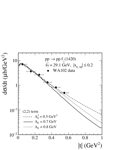
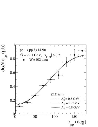
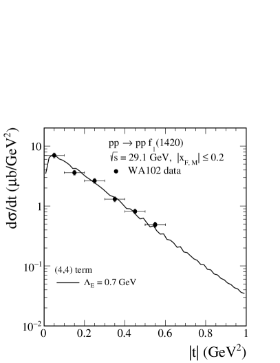
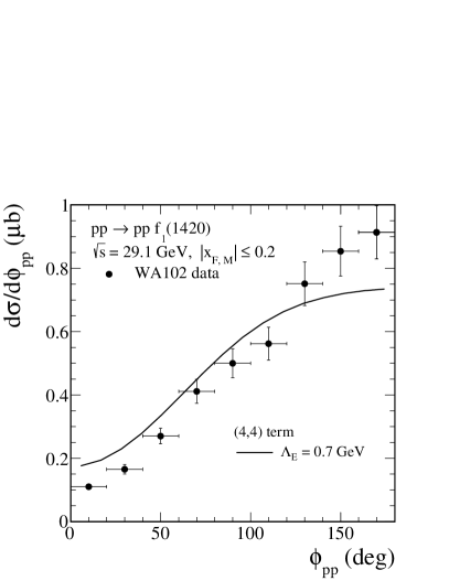
Figure 6: The $|t|$ (left panels) and $\phi_{pp}$ (right panels) distributions for the $pp\to ppf_{1}(1420)$ reaction at $\sqrt{s}=29.1$ GeV and $|x_{F,M}|\leqslant 0.2$. The theoretical results and the WA102 data points from Barberis:1998by have been normalised to the mean value of the total cross section (33). The error bars on the data correspond to the error on $\sigma_{\rm exp.}$ in (33). The separate individual coupling contributions for different cutoff parameters are shown. The absorption effects are included in the calculations. The oscillations in the left bottom panel are of numerical origin.

To summarize, we have seen in this section that $\mathbb{P}\mathbb{P}$ fusion with suitable $\mathbb{P}\mathbb{P}f_{1}$ couplings can give a reasonable description of the WA102 data. We have also seen that with the distributions explored it is very hard to discriminate between the various possible couplings, that is, to see which combination of coupling constants is preferred experimentally. In addition we have the problem that at the relatively low c.m. energy of $\sqrt{s}=29.1$ GeV subleading reggeon exchanges may still be rather important. This topic will be dealt with in Appendix D.

In the next sections we shall show our results for RHIC and LHC energies where subleading reggeon exchanges should be negligible, at least, for the midrapidity region. For these results we shall use the $\mathbb{P}\mathbb{P}f_{1}$ couplings as determined in the present section. But we must emphasize that our results for the RHIC and LHC obtained in this way should be considered as upper limits of the cross sections. If at the WA102 energies there are important contributions from subleading reggeon exchanges, the cross sections at the RHIC and LHC energies could be significantly smaller. As we discuss in Appendix D, we estimate that the reduction could be by a factor of up to 4 relative to the predictions given below.

III.2 Predictions for the LHC experiments

Now we wish to show our results (predictions) for the LHC.

Here we consider only the $\mathbb{P}\mathbb{P}$ fusion with the coupling parameters found in Sec. III.1 from the comparison with the WA102 data.

In Table 3 we have collected cross sections in $\mu$b for the reactions $pp\to ppf_{1}(1285)$ and $pp\to ppf_{1}(1420)$ at $\sqrt{s}=13$ TeV. We show results for some kinematical cuts on the rapidity of the mesons, $|{\rm y_{M}}|<2.5$, and also with an extra cut on momenta of leading protons $0.17\;{\rm GeV}<|p_{y,p}|<0.50\;{\rm GeV}$ that will be applied when using the ALFA subdetector on both sides of the ATLAS detector. We also show results for larger (forward) rapidities and without a measurement of outgoing protons relevant for the LHCb experiment. The calculations have been done in the Born approximation and with the absorption corrections included. For the $f_{1}(1285)$ we show the individual results for the $(l,S)=(2,2)$ and $(4,4)$ terms with $g^{\prime}_{\mathbb{P}\mathbb{P}f_{1}(1285)}=4.89$ in (11) and $g^{\prime\prime}_{\mathbb{P}\mathbb{P}f_{1}(1285)}=10.31$ in (12); see (27) and (28), respectively. For the $(\varkappa^{\prime},\varkappa^{\prime\prime})$ terms, (66) plus (67), we use (25). We have taken here the form factor (15) with $\Lambda_{E}=0.7$ GeV. For the $f_{1}(1420)$ we show the results for the $(l,S)=(2,2)$ term with $g^{\prime}_{\mathbb{P}\mathbb{P}f_{1}}=2.39$, see (35), and the $(\varkappa^{\prime},\varkappa^{\prime\prime})$ option from (34). As we see from comparing the last two columns of Table 3 the absorption effects lead to a sizeable reduction of the cross sections compared to the Born results.

Table 3: The integrated cross sections in $\mu$b for CEP of $f_{1}$ mesons in $pp$ collisions for $\sqrt{s}=13$ TeV for some kinematical cuts on the rapidity ${\rm y_{M}}$ of the meson, and also when limitations on the outgoing protons are imposed. The results for the $(l,S)=(2,2)$ and $(4,4)$ terms calculated from (11) and (12), respectively, and for the $\varkappa^{\prime}$ plus $\varkappa^{\prime\prime}$ terms calculated with the vertices (66) plus (67) are shown. The parameter values for $(\varkappa^{\prime},\varkappa^{\prime\prime})$ are taken from (25) for the $f_{1}(1285)$ and from (34) for the $f_{1}(1420)$. We have taken here the form factor (15) with $\Lambda_{E}=0.7$ GeV. The results without and with absorption effects are presented.

Meson	Cuts	Contribution	Parameters	$\sigma_{{\rm Born}}$ ($\mu$b)	$\sigma_{{\rm abs.}}$ ($\mu$b)
$f_{1}(1285)$	$|{\rm y_{M}}|<1.0$	$(2,2)$	Eq. (27)	36.11	14.83
		$(4,4)$	Eq. (28)	32.95	13.82
		$(\varkappa^{\prime},\varkappa^{\prime\prime})$	$\varkappa^{\prime\prime}/\varkappa^{\prime}=-6.25\;{\rm GeV}^{-2}$	27.17	18.63
		$(\varkappa^{\prime},\varkappa^{\prime\prime})$	$\varkappa^{\prime\prime}/\varkappa^{\prime}=-2.44\;{\rm GeV}^{-2}$	34.25	17.54
		$(\varkappa^{\prime},\varkappa^{\prime\prime})$	$\varkappa^{\prime\prime}/\varkappa^{\prime}=-1.0\;{\rm GeV}^{-2}$	36.27	16.56
	$|{\rm y_{M}}|<2.5$	$(2,2)$	Eq. (27)	90.63	37.54
		$(4,4)$	Eq. (28)	83.97	34.01
		$(\varkappa^{\prime},\varkappa^{\prime\prime})$	$\varkappa^{\prime\prime}/\varkappa^{\prime}=-6.25\;{\rm GeV}^{-2}$	69.08	45.79
		$(\varkappa^{\prime},\varkappa^{\prime\prime})$	$\varkappa^{\prime\prime}/\varkappa^{\prime}=-2.44\;{\rm GeV}^{-2}$	86.05	43.44
		$(\varkappa^{\prime},\varkappa^{\prime\prime})$	$\varkappa^{\prime\prime}/\varkappa^{\prime}=-1.0\;{\rm GeV}^{-2}$	91.47	41.00
	$|{\rm y_{M}}|<2.5$,	$(2,2)$	Eq. (27)	19.37	6.46
	$0.17\;{\rm GeV}<|p_{y,p}|<0.50\;{\rm GeV}$	$(4,4)$	Eq. (28)	18.07	6.06
		$(\varkappa^{\prime},\varkappa^{\prime\prime})$	$\varkappa^{\prime\prime}/\varkappa^{\prime}=-6.25\;{\rm GeV}^{-2}$	11.64	7.14
		$(\varkappa^{\prime},\varkappa^{\prime\prime})$	$\varkappa^{\prime\prime}/\varkappa^{\prime}=-2.44\;{\rm GeV}^{-2}$	16.71	7.10
		$(\varkappa^{\prime},\varkappa^{\prime\prime})$	$\varkappa^{\prime\prime}/\varkappa^{\prime}=-1.0\;{\rm GeV}^{-2}$	19.71	7.09
	$2.0<{\rm y_{M}}<4.5$	$(2,2)$	Eq. (27)	46.63	18.89
		$(4,4)$	Eq. (28)	43.58	18.07
		$(\varkappa^{\prime},\varkappa^{\prime\prime})$	$\varkappa^{\prime\prime}/\varkappa^{\prime}=-6.25\;{\rm GeV}^{-2}$	35.32	23.13
		$(\varkappa^{\prime},\varkappa^{\prime\prime})$	$\varkappa^{\prime\prime}/\varkappa^{\prime}=-2.44\;{\rm GeV}^{-2}$	44.28	22.14
		$(\varkappa^{\prime},\varkappa^{\prime\prime})$	$\varkappa^{\prime\prime}/\varkappa^{\prime}=-1.0\;{\rm GeV}^{-2}$	46.52	20.50
$f_{1}(1420)$	$|{\rm y_{M}}|<1.0$	$(2,2)$	Eq. (35)	8.80	3.66
		$(\varkappa^{\prime},\varkappa^{\prime\prime})$	$\varkappa^{\prime\prime}/\varkappa^{\prime}=-1.0\;{\rm GeV}^{-2}$	8.75	4.10
	$|{\rm y_{M}}|<2.5$	$(2,2)$	Eq. (35)	22.22	9.20
		$(\varkappa^{\prime},\varkappa^{\prime\prime})$	$\varkappa^{\prime\prime}/\varkappa^{\prime}=-1.0\;{\rm GeV}^{-2}$	22.16	9.85
	$|{\rm y_{M}}|<2.5$,	$(2,2)$	Eq. (35)	5.14	1.77
	$0.17\;{\rm GeV}<|p_{y,p}|<0.50\;{\rm GeV}$	$(\varkappa^{\prime},\varkappa^{\prime\prime})$	$\varkappa^{\prime\prime}/\varkappa^{\prime}=-1.0\;{\rm GeV}^{-2}$	4.65	1.67
	$2.0<{\rm y_{M}}<4.5$	$(2,2)$	Eq. (35)	11.37	4.68
		$(\varkappa^{\prime},\varkappa^{\prime\prime})$	$\varkappa^{\prime\prime}/\varkappa^{\prime}=-1.0\;{\rm GeV}^{-2}$	11.35	4.92

In Fig. 8 we show our predictions for the $pp\to ppf_{1}(1285)$ reaction for $\sqrt{s}=13$ TeV, $|{\rm y_{M}}|<2.5$, and for the cut on the leading protons of $0.17\;{\rm GeV}<|p_{y,p}|<0.50\;{\rm GeV}$. Here the distribution of $p_{t,M}$ does not require, whereas those of $\phi_{pp}$, $|t|$, and ${\rm dP_{t}}$ do require the detection of the leading protons. The results calculated with the vertices (11) [$(2,2)$ term], (12) [$(4,4)$ term], and (66) plus (67) [$\varkappa^{\prime\prime}/\varkappa^{\prime}=-1$ GeV² and $-2.44$ GeV²] give quite similar distributions. The contribution with $\varkappa^{\prime\prime}/\varkappa^{\prime}=-6.25$ GeV² gives a significantly different shape in the distributions of $\phi_{pp}$ and of the transverse momentum of the $f_{1}(1285)$.

In all cases the absorption effects are included. Inclusion of absorption effects modifies the differential distributions because their shapes depend on the kinematics of outgoing protons. We have checked numerically that the absorption effects decrease the distributions mostly at higher values of the variables $\phi_{pp}$ and ${\rm dP_{t}}$ and at smaller values of $p_{t,M}$ and $|t|$. The measurement of such distributions would allow one to better understand absorption effects. This could be tested in future in experiments at the LHC, when both protons are measured, such as ATLAS-ALFA and CMS-TOTEM. The GenEx Kycia:2014hea ; Kycia:2017ota and GRANIITTI Mieskolainen:2019jpv Monte Carlo event generators could be used in this context.

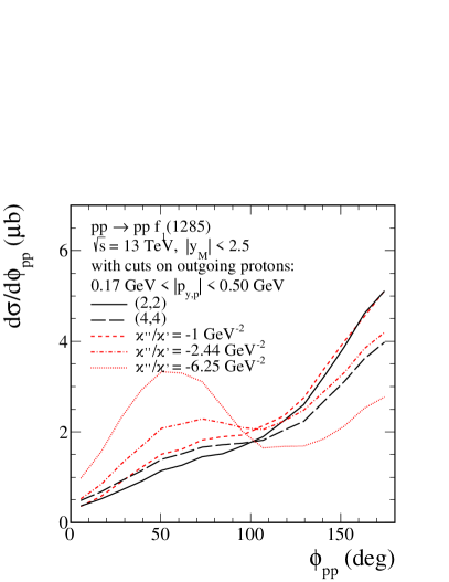
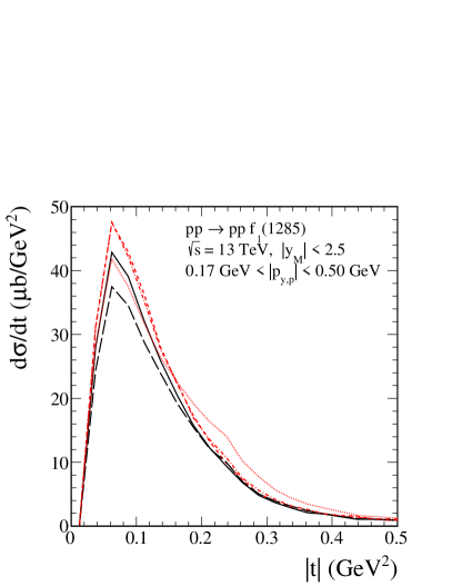
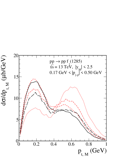
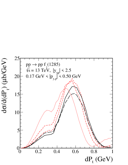
Figure 8: The differential cross sections for the $f_{1}(1285)$ production at $\sqrt{s}=13$ TeV and $|{\rm y_{M}}|<2.5$. The results for $(l,S)=(2,2)$, $(4,4)$, and $(\varkappa^{\prime},\varkappa^{\prime\prime})$ contributions are shown. Here we use for the $(2,2)$ and $(4,4)$ terms (27) and (28), respectively. For the $(\varkappa^{\prime},\varkappa^{\prime\prime})$ terms we use (25). The absorption effects are included in all the calculations.

Now we discuss one of the most prominent decay modes of the $f_{1}(1285)$, the decay $f_{1}(1285)\to\pi^{+}\pi^{-}\pi^{+}\pi^{-}$. This four-pion decay channel seems well suited to measure the $f_{1}(1285)$ meson in CEP. However, the $f_{1}(1285)$ is rather close in mass to the $f_{2}(1270)$ which also decays into four pions. In principle, the $f_{1}(1285)$ and $f_{2}(1270)$ decays will interfere in the four-pion final state. Note that this interference could be used to determine the relative sign of the $f_{1}$ and $f_{2}$ production times decay amplitudes. But the interference terms will drop out in the total decay rates.

In PDG Tanabashi:2018oca the following branching fractions are listed:

$${\cal BR}(f_{1}(1285)\to\pi^{+}\pi^{-}\pi^{+}\pi^{-})=(11.2^{+0.7}_{-0.6})\,\%\,,$$ (42)

$${\cal BR}(f_{2}(1270)\to\pi^{+}\pi^{-}\pi^{+}\pi^{-})=(2.8\pm 0.4)\,\%\,.$$ (43)

Note that $\Gamma(f_{2}(1270))=186.7^{+2.2}_{-2.5}$ MeV, $\Gamma(f_{1}(1285))=(22.7\pm 1.1)$ MeV. Thus we have $\Gamma(f_{2}(1270))\gg\Gamma(f_{1}(1285))$.

In the following, for CEP of the $f_{1}(1285)$ meson, we assume the $(l,S)=(2,2)$ coupling and $\Lambda_{E}=0.7$ GeV; see (27) and $\sigma_{{\rm abs.}}$ in Table 3. For CEP of the $f_{2}(1270)$ meson the cross section is $\sigma_{pp\to ppf_{2}(1270)}=11.25$ $\mu$b with the parameters from Ref. Lebiedowicz:2019por : $(g_{\mathbb{P}\mathbb{P}f_{2}}^{(2)},g_{\mathbb{P}\mathbb{P}f_{2}}^{(5)})=(-4.0,16.0)$, $\Lambda_{0}^{2}=0.5$ GeV². The absorption effects are taken into account in the calculation. We obtain the integrated cross sections for $\sqrt{s}=13$ TeV and $|{\rm y_{M}}|<2.5$, including the PDG branching fractions (42) and (43), as follows

$$\sigma_{pp\to ppf_{1}(1285)}\times{\cal BR}(f_{1}(1285)\to\pi^{+}\pi^{-}\pi^{+}\pi^{-})=4.20\;\mu{\rm b}$$ (44)

and

$$\sigma_{pp\to ppf_{2}(1270)}\times{\cal BR}(f_{2}(1270)\to\pi^{+}\pi^{-}\pi^{+}\pi^{-})=0.32\;\mu{\rm b}\;,$$ (45)

respectively. Thus we predict a large cross section for the exclusive axial-vector $f_{1}(1285)$ production compared to the production of the tensor $f_{2}(1270)$ meson in the $\pi^{+}\pi^{-}\pi^{+}\pi^{-}$ channel. Even if we scale down the $f_{1}$ cross section by a factor of 4, it will still be larger than our result for the $f_{2}$ cross section. In addition, $\Gamma(f_{2}(1270))\gg\Gamma(f_{1}(1285))$, so $f_{1}(1285)$ will be seen as a sharp peak on top of a smaller bump corresponding to the $f_{2}(1270)$.

III.3 Predictions for the STAR experiment at RHIC

The STAR experiments at RHIC measure CEP reactions at $\sqrt{s}=200$ GeV Adam:2020sap and at $\sqrt{s}=510$ GeV ICHEP_STAR . It has the possibility to observe the outgoing protons at least in a certain phase space region. We shall present the predictions of our model for the cut on the rapidity of the meson $|{\rm y_{M}}|<0.7$ and for limitations on the outgoing protons, for $\sqrt{s}=200$ GeV,

$$(p_{x,p}+0.3\;{\rm GeV})^{2}+p_{y,p}^{2}<0.25\;{\rm GeV}^{2}\,,$$

$$0.2\;{\rm GeV}<|p_{y,p}|<0.4\;{\rm GeV}\,,$$

$$p_{x,p}>-0.2\;{\rm GeV}\,,$$ (46)

as specified in Eq. (6.1) of Adam:2020sap , and for $\sqrt{s}=510$ GeV,

$$(p_{x,p}+0.6\;{\rm GeV})^{2}+p_{y,p}^{2}<1.25\;{\rm GeV}^{2}\,,$$

$$0.4\;{\rm GeV}<|p_{y,p}|<0.8\;{\rm GeV}\,,$$

$$p_{x,p}>-0.27\;{\rm GeV}\,,$$ (47)

as specified in ICHEP_STAR .

In Table 4 we give the analog of Table 3 but for the STAR experiments.

Table 4: The integrated cross sections in nb for CEP of $f_{1}$ mesons in $pp$ collisions for the STAR experiments for $|{\rm y_{M}}|<0.7$ and when in addition limitations on the outgoing protons are imposed; see Eq. (46) for $\sqrt{s}=200$ GeV and Eq. (47) for $\sqrt{s}=510$ GeV. The parameter values for $(\varkappa^{\prime},\varkappa^{\prime\prime})$ are taken from (25) for the $f_{1}(1285)$ and from (34) for the $f_{1}(1420)$. We have taken here the form factor (15) with $\Lambda_{E}=0.7$ GeV. The results without and with absorption effects are presented.

$\sqrt{s}$ (GeV)	Meson	Cuts	Contribution	Parameters	$\sigma_{{\rm Born}}$ (nb)	$\sigma_{{\rm abs.}}$ (nb)
200	$f_{1}(1285)$	$|{\rm y_{M}}|<0.7$,	$(2,2)$	Eq. (27)	204.2	127.5
		and Eq. (46)	$(4,4)$	Eq. (28)	163.7	103.1
			$(\varkappa^{\prime},\varkappa^{\prime\prime})$	$\varkappa^{\prime\prime}/\varkappa^{\prime}=-6.25\;{\rm GeV}^{-2}$	88.5	76.1
			$(\varkappa^{\prime},\varkappa^{\prime\prime})$	$\varkappa^{\prime\prime}/\varkappa^{\prime}=-2.44\;{\rm GeV}^{-2}$	178.8	122.8
			$(\varkappa^{\prime},\varkappa^{\prime\prime})$	$\varkappa^{\prime\prime}/\varkappa^{\prime}=-1.0\;{\rm GeV}^{-2}$	210.5	136.4
200	$f_{1}(1420)$	$|{\rm y_{M}}|<0.7$,	$(2,2)$	Eq. (35)	50.0	31.3
		and Eq. (46)	$(\varkappa^{\prime},\varkappa^{\prime\prime})$	$\varkappa^{\prime\prime}/\varkappa^{\prime}=-1.0\;{\rm GeV}^{-2}$	50.3	31.9
510	$f_{1}(1285)$	$|{\rm y_{M}}|<0.7$,	$(2,2)$	Eq. (27)	127.5	27.8
		and Eq. (47)	$(4,4)$	Eq. (28)	111.5	27.0
			$(\varkappa^{\prime},\varkappa^{\prime\prime})$	$\varkappa^{\prime\prime}/\varkappa^{\prime}=-6.25\;{\rm GeV}^{-2}$	98.9	89.4
			$(\varkappa^{\prime},\varkappa^{\prime\prime})$	$\varkappa^{\prime\prime}/\varkappa^{\prime}=-2.44\;{\rm GeV}^{-2}$	41.0	29.6
			$(\varkappa^{\prime},\varkappa^{\prime\prime})$	$\varkappa^{\prime\prime}/\varkappa^{\prime}=-1.0\;{\rm GeV}^{-2}$	90.3	26.3
510	$f_{1}(1420)$	$|{\rm y_{M}}|<0.7$,	$(2,2)$	Eq. (35)	30.7	6.8
		and Eq. (47)	$(\varkappa^{\prime},\varkappa^{\prime\prime})$	$\varkappa^{\prime\prime}/\varkappa^{\prime}=-1.0\;{\rm GeV}^{-2}$	21.3	6.2

In Fig. 9 we show as an example various predictions for $f_{1}(1285)$ CEP at $\sqrt{s}=200$ GeV, at $|{\rm y_{M}}|<0.7$, and with extra cuts on the leading protons (46). The experimental cuts have crucial influence on the shape of the differential distributions. In particular, the result that the distributions (nearly) vanish for certain values of the variables $\phi_{pp}$, $p_{t,M}$ and ${\rm dP_{t}}$ is caused by the specific cuts (46).

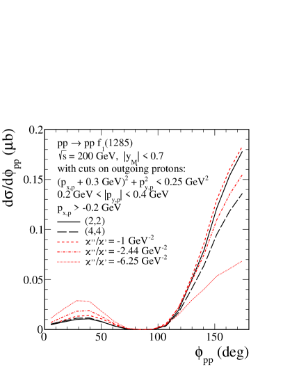
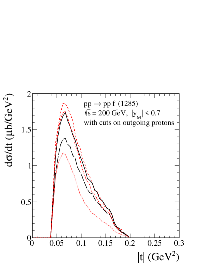
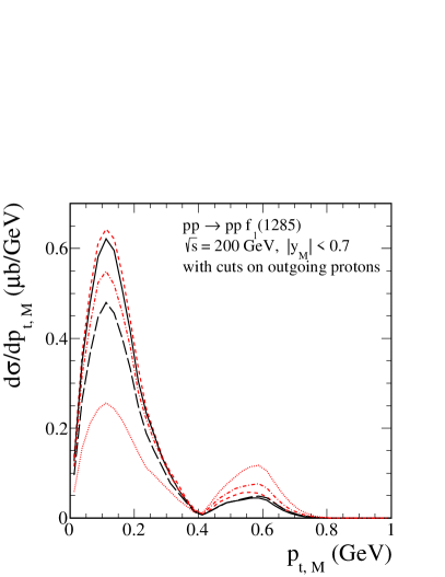
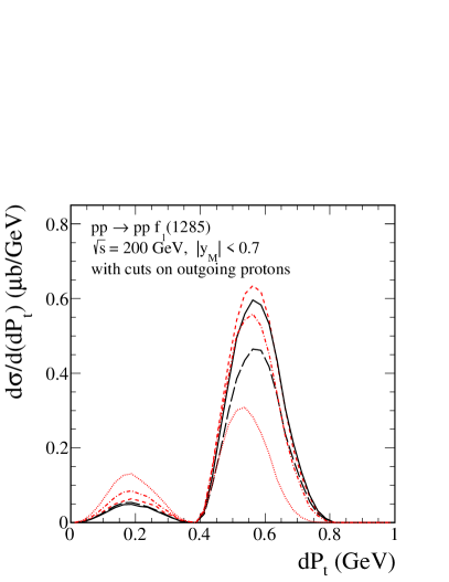
Figure 9: The differential cross sections for the $f_{1}(1285)$ production at $\sqrt{s}=200$ GeV for $|{\rm y_{M}}|<0.7$ and with cuts on the leading protons specified in (46). The meaning of the lines is the same as in Fig. 8. The absorption effects are included in all the calculations.

In Fig. 10 we show our predictions for $f_{1}(1285)$ CEP at $\sqrt{s}=510$ GeV, $|{\rm y_{M}}|<0.7$, and with extra cuts on the leading protons (47). The suppression of the differential cross sections $d\sigma/d\phi_{pp}$ close to $90^{\circ}$ is due to the specific cuts (47) applied to the forward scattered protons. The general situation for $d\sigma/d\phi_{pp}$ and $d\sigma/dt$ at $\sqrt{s}=510$ GeV is similar to that of $\sqrt{s}=200$ GeV but there are some noticeable differences due to the different cuts on the outgoing protons. A clear difference is seen for the option $\varkappa^{\prime\prime}/\varkappa^{\prime}=-6.25\;{\rm GeV}^{-2}$. This is due to the kinematics-dependent absorption effects.

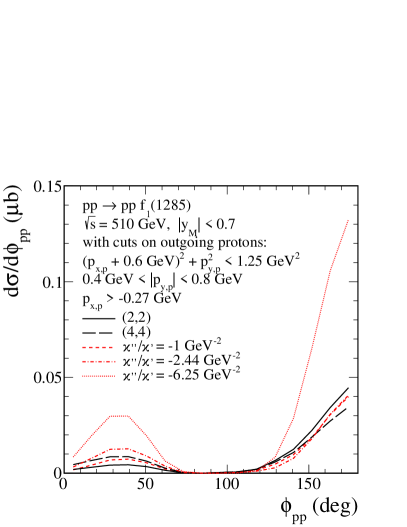
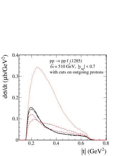
Figure 10: The differential cross sections for the $f_{1}(1285)$ production at $\sqrt{s}=510$ GeV for $|{\rm y_{M}}|<0.7$ and with cuts on the leading protons specified in (47). The meaning of the lines is the same as in Fig. 8. The absorption effects are included in all the calculations.

IV Conclusions

In this paper, we have discussed in detail the exclusive central production of the pseudovector $f_{1}(1285)$ and $f_{1}(1420)$ mesons in proton-proton collisions. The calculations for the $pp\to ppf_{1}(1285)$ and $pp\to ppf_{1}(1420)$ reactions have been performed in the tensor-pomeron approach Ewerz:2013kda . In general, two $\mathbb{P}\mathbb{P}f_{1}$ couplings with different orbital angular momentum and spin of two “pomeron particles” are possible, namely $(l,S)=(2,2)$ and $(4,4)$. We have presented explicitly amplitudes and formulas for the $\mathbb{P}\mathbb{P}f_{1}$ vertices as derived from corresponding coupling Lagrangians. Two different approaches for the $\mathbb{P}\mathbb{P}f_{1}$ coupling have been considered.

1. In the first approach, two independent $\mathbb{P}\mathbb{P}f_{1}$ coupling constants, $g^{\prime}_{\mathbb{P}\mathbb{P}f_{1}}$ and $g^{\prime\prime}_{\mathbb{P}\mathbb{P}f_{1}}$ that correspond to the $(l,S)=(2,2)$ and $(l,S)=(4,4)$ couplings [see Eqs. (11) and (12), respectively], not known a priori as they are of nonperturbative origin, have been fitted to existing data from the WA102 experiment. A reasonable agreement with the WA102 data can be obtained with either a pure $(l,S)=(2,2)$ or a pure $(l,S)=(4,4)$ coupling.

2. The second approach is based on holographic QCD, namely the (chiral) Sakai-Sugimoto model, where the pomeron-pomeron-$f_{1}$ couplings (61) and (62) are obtained from a Chern-Simons action representing the mixed axial-gravitational anomaly of QCD. This also involves two coupling constants, with a prediction for their ratio in terms of the Kaluza-Klein mass scale of the model as given by (24). Comparing the $\phi_{pp}$ distribution for different values of this ratio confirms the sign of this ratio as predicted by the Sakai-Sugimoto model, but not its magnitude. However, freely fitting the magnitude of the couplings, reasonable agreement with the WA102 data is again obtained.

Assuming that the WA102 data are already dominated by pomeron exchanges, we have presented various predictions for experiments at the RHIC and the LHC. The total cross sections and several differential distributions for the $pp\to ppf_{1}(1285)$ reaction have been presented. In our opinion the $\pi^{+}\pi^{-}\pi^{+}\pi^{-}$ channel seems the best to observe $f_{1}(1285)$ for both the RHIC and the LHC experiments. We have shown that independent of the $\mathbb{P}\mathbb{P}f_{1}$ coupling decomposition the cross section for the $pp\to pp(f_{1}(1285)\to\pi^{+}\pi^{-}\pi^{+}\pi^{-})$ reaction is much larger than for the $pp\to pp(f_{2}(1270)\to\pi^{+}\pi^{-}\pi^{+}\pi^{-})$ reaction. As the $f_{1}(1285)$ has a much narrower width than the $f_{2}(1270)$ it would be seen in the mass distribution as a narrow peak on a somewhat broader bump corresponding to the $f_{2}(1270)$.

The question can be asked if CEP of the $f_{1}(1285)$ and $f_{1}(1420)$ mesons may be confounded in experiments with CEP of $\eta$-type mesons which are nearby in mass. The $f_{1}(1285)$ and the $\eta(1295)$ are close in mass. For the $f_{1}(1420)$ we have the $\eta(1405)$ and the $\eta(1475)$ as potential background candidates. 

Let us first discuss the $f_{1}(1285)$ and $\eta(1295)$ issue. These two mesons have a common decay mode ($\eta\pi\pi$) but only the $f_{1}(1285)$ decays to $4\pi$ and $K\bar{K}\pi$ Tanabashi:2018oca . Thus, concentrating in an experiment on these latter final states there can be no confusion between the $f_{1}(1285)$ and the $\eta(1295)$.

For the $f_{1}(1420)$ and the nearby $f_{1}(1405)$ and $\eta(1475)$ mesons things are more complicated. The channel where the $f_{1}(1420)$ is to be observed is $K\bar{K}\pi$, and this channel is also prominent for the $\eta(1405)$ and $\eta(1475)$ decays. Thus, here experimentalists will have to rely on precise mass measurements and partial-wave analyses in order to distinguish $f_{1}$- and $\eta$-type resonances. Now we discuss that the distributions in the azimuthal angle $\phi_{pp}$ between the transverse momenta of the outgoing protons may also be used to disentangle $f_{1}$ and $\eta$ contributions. In Appendix E we show that for CEP of an $\eta$-type meson at high energies $\sqrt{s}$ the $\phi_{pp}$ distribution must vanish for $\phi_{pp}=0$ and $\phi_{pp}=\pi$. For CEP of an $f_{1}$ meson there is no such restriction and, indeed, the $\phi_{pp}$ distributions measured by the WA102 Collaboration are nonzero for $\phi_{pp}=0$ and $\phi_{pp}=\pi$; see Figs. 2, 5, and 6.

Our predictions can be tested by the STAR Collaboration at RHIC and by all collaborations (ALICE, ATLAS, CMS, LHCb) working at the LHC.

In all cases considered we have included absorption effects. We have found that the absorption effects strongly depend on kinematics, i.e., also on experimental cuts, as well as on the type of the $\mathbb{P}\mathbb{P}f_{1}$ coupling used in the calculation. Different tensorial couplings discussed in the present paper lead to different dependences on $t_{1}$ and $t_{2}$ which are crucial for the size of absorption effects. The effect of absorption was not the primary aim of this study; therefore, the discussion of this point was kept rather short in our present paper.

To summarize, we think that a study of CEP of the axial vector mesons $f_{1}$ should be quite rewarding for experimentalists. We have analysed in detail the results of the WA102 experiment which worked at $\sqrt{s}=29.1$ GeV, and we have shown that we get a good description of the results with the pomeron-pomeron fusion mechanism. Such studies could be extended, for instance by the COMPASS experiment Abbon:2014aex ; Ketzer:2019wmd , where presumably one could study the influence of reggeon-pomeron and reggeon-reggeon fusion terms. At high energies, at RHIC and LHC, pomeron-pomeron fusion is expected to dominate. We have given predictions for CEP of $f_{1}$ mesons there. Comparing them with future experimental results should allow a good determination of the $\mathbb{P}\mathbb{P}f_{1}$ coupling constants. These are nonperturbative QCD parameters. Their theoretical calculation is a challenge. The holographic methods applied to QCD already give some predictions here, as we have shown in our paper. We can envisage a fruitful interplay of experiment and theory in this field in the future leading finally to a satisfactory picture of the couplings of two pomerons to the axial vector $f_{1}$ mesons studied here and, quite generally, to single mesons.

Appendix A The coupling of an $f_{1}$-type meson to two pomerons

Here we study the coupling of a meson $f_{1}$ with $I^{G}J^{PC}=0^{+}1^{++}$ to two tensor pomerons. We use the relations for the tensor pomeron from Ewerz:2013kda ; Lebiedowicz:2013ika .

In Appendix A of Lebiedowicz:2013ika the fictitious reaction of two “real spin-2 pomerons“ annihilating to a meson was studied. This was done in order to get an idea what type of pomeron-pomeron-meson ($\mathbb{P}\mathbb{P}M$) couplings we would have to expect. Looking at Table 6 of Lebiedowicz:2013ika we see that for the production of a $J^{P}=1^{+}$ meson we can have the following values of angular momentum $l$ and total spin $S$ of the two tensor pomerons:

$$(l,S)=(2,2)\,,\;(4,4)\,.$$ (48)

We find only these two possibilities.

The task is now to construct $\mathbb{P}\mathbb{P}f_{1}$ coupling Lagrangians which, applied to the above “real spin-2 pomeron” annihilation, give the $(l,S)=(2,2)$ and $(4,4)$ amplitudes. We emphasize that such constructions are not unique. We give in our paper, in this and the following appendix, two possibilities for such constructions and we discuss their relations. Here we shall rely on the experience gained with the construction of pomeron-pomeron-meson couplings in Ewerz:2013kda ; Ewerz:2016onn ; Lebiedowicz:2013ika ; Lebiedowicz:2014bea ; Lebiedowicz:2016ioh ; Lebiedowicz:2016ryp ; Lebiedowicz:2018eui ; Lebiedowicz:2016zka ; Lebiedowicz:2018sdt ; Lebiedowicz:2019jru ; Lebiedowicz:2019boz . We want to couple two spin 2 pomeron fields $\mathbb{P}_{\kappa\lambda}$ to the $f_{1}$ vector field $U_{\alpha}$ which is, in equations, conveniently represented by an antisymmetric second-rank tensor field $\partial_{\alpha}U_{\beta}-\partial_{\beta}U_{\alpha}$. The $l$ values of the couplings should be reflected by $l$ derivatives. Using these heuristic principles it is not difficult to write down $\mathbb{P}\mathbb{P}f_{1}$ couplings which fulfil all required properties.

In the following we shall first construct the $\mathbb{P}\mathbb{P}f_{1}$ coupling corresponding to $(l,S)=(2,2)$. For this we define the following rank 8 tensor function:

$$\Gamma^{(8)}_{\kappa\lambda,\rho\sigma,\mu\nu,\alpha\beta} = g_{\kappa\rho}g_{\mu\sigma}\varepsilon_{\lambda\nu\alpha\beta}+g_{\lambda\rho}g_{\mu\sigma}\varepsilon_{\kappa\nu\alpha\beta}+g_{\kappa\sigma}g_{\mu\rho}\varepsilon_{\lambda\nu\alpha\beta}+g_{\lambda\sigma}g_{\mu\rho}\varepsilon_{\kappa\nu\alpha\beta}$$ (49)

$$+g_{\kappa\rho}g_{\mu\lambda}\varepsilon_{\sigma\nu\alpha\beta}+g_{\sigma\kappa}g_{\mu\lambda}\varepsilon_{\rho\nu\alpha\beta}+g_{\rho\lambda}g_{\mu\kappa}\varepsilon_{\sigma\nu\alpha\beta}+g_{\sigma\lambda}g_{\mu\kappa}\varepsilon_{\rho\nu\alpha\beta}$$

$$-g_{\kappa\lambda}g_{\mu\rho}\varepsilon_{\sigma\nu\alpha\beta}-g_{\kappa\lambda}g_{\mu\sigma}\varepsilon_{\rho\nu\alpha\beta}-g_{\kappa\mu}g_{\rho\sigma}\varepsilon_{\lambda\nu\alpha\beta}-g_{\lambda\mu}g_{\rho\sigma}\varepsilon_{\kappa\nu\alpha\beta}$$

$$+(\mu\leftrightarrow\nu)\,.$$

For the Levi-Civita symbol we use the normalisation $\varepsilon_{0123}=+1$.

It can be checked that $\Gamma^{(8)}$ satisfies the following relations:

$$\Gamma^{(8)}_{\kappa\lambda,\rho\sigma,\mu\nu,\alpha\beta}=\Gamma^{(8)}_{\lambda\kappa,\rho\sigma,\mu\nu,\alpha\beta}=\Gamma^{(8)}_{\kappa\lambda,\sigma\rho,\mu\nu,\alpha\beta}$$

$$\qquad\qquad\qquad=\Gamma^{(8)}_{\kappa\lambda,\rho\sigma,\nu\mu,\alpha\beta}=\Gamma^{(8)}_{\rho\sigma,\kappa\lambda,\mu\nu,\alpha\beta}=-\Gamma^{(8)}_{\kappa\lambda,\rho\sigma,\mu\nu,\beta\alpha}\,;$$ (50)

$$\Gamma^{(8)}_{\kappa\lambda,\rho\sigma,\mu\nu,\alpha\beta}\,g^{\kappa\lambda}=0\,,$$

$$\Gamma^{(8)}_{\kappa\lambda,\rho\sigma,\mu\nu,\alpha\beta}\,g^{\rho\sigma}=0\,,$$

$$\Gamma^{(8)}_{\kappa\lambda,\rho\sigma,\mu\nu,\alpha\beta}\,g^{\mu\nu}=0\,.$$ (51)

Now we define the $\mathbb{P}\mathbb{P}f_{1}$ coupling corresponding to $(l,S)=(2,2)$ as follows

$${\cal L}^{\prime}_{\mathbb{P}\mathbb{P}f_{1}}(x)=\frac{g^{\prime}_{\mathbb{P}\mathbb{P}f_{1}}}{32\,M_{0}^{2}}\Big{(}\mathbb{P}_{\kappa\lambda}(x)\Big{(}\stackrel{{\scriptstyle\leftrightarrow}}{{\partial}}_{\!\mu}\,\stackrel{{\scriptstyle\leftrightarrow}}{{\partial}}_{\!\nu}\Big{)}\mathbb{P}_{\rho\sigma}(x)\Big{)}\Big{(}\partial_{\alpha}U_{\beta}(x)-\partial_{\beta}U_{\alpha}(x)\Big{)}\,\Gamma^{(8)\,\kappa\lambda,\rho\sigma,\mu\nu,\alpha\beta}\,.\qquad$$ (52)

Here $\mathbb{P}_{\kappa\lambda}(x)$ is the effective field of the pomeron and $U_{\alpha}(x)$ the field of the $f_{1}$ meson. Furthermore we have introduced, for dimensional reasons, in (52) a factor $M_{0}^{-2}$ with $M_{0}=1$ GeV, and then $g^{\prime}_{\mathbb{P}\mathbb{P}f_{1}}$ is a dimensionless coupling constant. The asymmetric derivative has the form $\stackrel{{\scriptstyle\leftrightarrow}}{{\partial}}_{\!\mu}=\stackrel{{\scriptstyle\rightarrow}}{{\partial}}_{\!\mu}-\stackrel{{\scriptstyle\leftarrow}}{{\partial}}_{\!\mu}$. The $\mathbb{P}$ effective field satisfies the identities

$$\mathbb{P}_{\kappa\lambda}(x)=\mathbb{P}_{\lambda\kappa}(x)\,,$$

$$g^{\kappa\lambda}\,\mathbb{P}_{\kappa\lambda}(x)=0\,.$$ (53)

From (52) we get the “bare” $\mathbb{P}\mathbb{P}f_{1}$ vertex (11).

Now we shall set up the $\mathbb{P}\mathbb{P}f_{1}$ coupling corresponding to $(l,S)=(4,4)$:

$${\cal L}^{\prime\prime}_{\mathbb{P}\mathbb{P}f_{1}}(x) = \frac{g^{\prime\prime}_{\mathbb{P}\mathbb{P}f_{1}}}{24\cdot 32\cdot M_{0}^{4}}\Big{(}\mathbb{P}_{\kappa\lambda}(x)\Big{(}\stackrel{{\scriptstyle\leftrightarrow}}{{\partial}}_{\!\mu_{1}}\,\stackrel{{\scriptstyle\leftrightarrow}}{{\partial}}_{\!\mu_{2}}\,\stackrel{{\scriptstyle\leftrightarrow}}{{\partial}}_{\!\mu_{3}}\,\stackrel{{\scriptstyle\leftrightarrow}}{{\partial}}_{\!\mu_{4}}\Big{)}\mathbb{P}_{\rho\sigma}(x)\Big{)}\Big{(}\partial_{\alpha}U_{\beta}(x)-\partial_{\beta}U_{\alpha}(x)\Big{)}$$ (54)

$$\times\Gamma^{(10)\,\kappa\lambda,\rho\sigma,\mu_{1}\mu_{2}\mu_{3}\mu_{4},\alpha\beta}\,.$$

Here we define the rank 10 tensor function

$$\Gamma^{(10)}_{\kappa\lambda,\rho\sigma,\mu_{1}\mu_{2}\mu_{3}\mu_{4},\alpha\beta} = \left.\Big{\{}\Bigl{[}\Bigl{(}g_{\kappa\mu_{1}}g_{\lambda\mu_{2}}-\frac{1}{4}g_{\kappa\lambda}g_{\mu_{1}\mu_{2}}\Bigr{)}\Bigl{(}g_{\rho\mu_{3}}\varepsilon_{\sigma\mu_{4}\alpha\beta}-\frac{1}{4}g_{\rho\sigma}\varepsilon_{\mu_{3}\mu_{4}\alpha\beta}\Bigr{)}\right.$$ (55)

$$\left.+(\kappa\leftrightarrow\lambda)+(\rho\leftrightarrow\sigma)+(\kappa\leftrightarrow\lambda,\rho\leftrightarrow\sigma)\Bigr{]}+(\kappa,\lambda)\leftrightarrow(\rho,\sigma)\Big{\}}\right.$$

$$+\;{\rm all\;permutation\;of}\;\mu_{1},\mu_{2},\mu_{3},\mu_{4}\,.$$

$\Gamma^{(10)}$ (55) has the following properties:

$$\Gamma^{(10)}_{\kappa\lambda,\rho\sigma,\mu_{1}\mu_{2}\mu_{3}\mu_{4},\alpha\beta}=\Gamma^{(10)}_{\lambda\kappa,\rho\sigma,\mu_{1}\mu_{2}\mu_{3}\mu_{4},\alpha\beta}=\Gamma^{(10)}_{\kappa\lambda,\sigma\rho,\mu_{1}\mu_{2}\mu_{3}\mu_{4},\alpha\beta}$$

$$\qquad\qquad\qquad\qquad\;=\Gamma^{(10)}_{\rho\sigma,\kappa\lambda,\mu_{1}\mu_{2}\mu_{3}\mu_{4},\alpha\beta}=-\Gamma^{(10)}_{\kappa\lambda,\rho\sigma,\mu_{1}\mu_{2}\mu_{3}\mu_{4},\beta\alpha}\,,$$ (56)

$$\Gamma^{(10)}_{\kappa\lambda,\rho\sigma,\mu_{1}\mu_{2}\mu_{3}\mu_{4},\alpha\beta}\;{\rm is\;totally\;symmetric\;in}\;\mu_{1},\mu_{2},\mu_{3},\mu_{4}\,,$$ (57)

$$\Gamma^{(10)}_{\kappa\lambda,\rho\sigma,\mu_{1}\mu_{2}\mu_{3}\mu_{4},\alpha\beta}\,g^{\kappa\lambda}=0\,,$$

$$\Gamma^{(10)}_{\kappa\lambda,\rho\sigma,\mu_{1}\mu_{2}\mu_{3}\mu_{4},\alpha\beta}\,g^{\rho\sigma}=0\,.$$ (58)

In (54) $g^{\prime\prime}_{\mathbb{P}\mathbb{P}f_{1}}$ is a dimensionless coupling constant. From (54)–(58) we get the “bare” $\mathbb{P}\mathbb{P}f_{1}$ vertex (12).

Appendix B Different forms for the $\mathbb{P}\mathbb{P}f_{1}$ coupling as obtained in holographic QCD

In (52) and (54) of Appendix A we have given a possible form for the $\mathbb{P}\mathbb{P}f_{1}$ couplings. In the holographic framework another form is obtained. In the Sakai-Sugimoto model Sakai:2004cn ; Sakai:2005yt , the coupling of singlet pseudoscalar and axial-vector mesons to two tensor glueballs is determined by the gravitational CS action (describing axial-gravitational anomalies), as given in Eq. (59) of Anderson:2014jia ,

$$S_{{\rm CS}} \supset \frac{N_{c}}{1536\pi^{2}}\int d^{5}x\epsilon^{MNPQR}\text{Tr}(A_{M})R_{NPST}R_{QR}^{\quad TS}.$$ (59)

The (singlet component of the) axial-vector meson is contained in $\text{Tr}(A_{\mu})=A_{\mu}^{(0)}=U_{\mu}(x)\psi(Z)$, leading to

$$S_{{\rm CS}} \supset \frac{N_{c}}{384\pi^{2}}\sqrt{\frac{N_{f}}{2}}\int d^{5}x\epsilon^{\mu\nu\rho\sigma}A_{\mu}^{(0)}R_{Z\nu ST}R_{\rho\sigma}^{\quad TS},$$ (60)

where $Z$ refers to the holographic direction.

Five-dimensional gravitons correspond to four-dimensional tensor glueballs, and their coupling to $f_{1}$ is obtained by expanding this term to second order in transverse-traceless metric perturbations and integrating over radial wave functions. Using the same notation as in Appendix A we derive the coupling Lagrangians,

$${\cal L}_{\rm CS}^{\prime}(x)=\varkappa^{\prime}\,U_{\alpha}(x)\,\varepsilon^{\alpha\beta\gamma\delta}\,\mathbb{P}^{\mu}_{\;\;\beta}(x)\,\partial_{\delta}\mathbb{P}_{\gamma\mu}(x)\,,$$ (61)

$${\cal L}_{\rm CS}^{\prime\prime}(x)=\varkappa^{\prime\prime}\,U_{\alpha}(x)\,\varepsilon^{\alpha\beta\gamma\delta}\,\Bigl{(}\partial_{\nu}\mathbb{P}^{\mu}_{\;\;\beta}(x)\Bigr{)}\Bigl{(}\partial_{\delta}\partial_{\mu}\mathbb{P}^{\nu}_{\;\;\gamma}(x)-\partial_{\delta}\partial^{\nu}\mathbb{P}_{\gamma\mu}(x)\Bigr{)}\,,$$ (62)

where

$$\varkappa^{\prime} = -\frac{4.872\,\mathcal{N}\sqrt{N_{f}}}{\sqrt{N_{c}^{3}\lambda^{3}}}\,,$$ (63)

$$\varkappa^{\prime\prime} = \frac{27.434\,\mathcal{N}\sqrt{N_{f}}}{M_{\text{KK}}^{2}\sqrt{N_{c}^{3}\lambda^{3}}}$$ (64)

and $\mathcal{N}$ is a normalization constant that we leave undetermined because of the ambiguities Anderson:2014jia in the reggeization of the tensor glueball into pomerons (it would be unity for a purely flavour-singlet axial-vector meson when $\mathbb{P}_{\mu\nu}$ was replaced by the tensor glueball $T_{\mu\nu}$ normalized as in Brunner:2015oqa ).

The Sakai-Sugimoto model has two free parameters, a Kaluza-Klein mass scale $M_{\text{KK}}$ and the dimensionless ’t Hooft coupling $\lambda$ at this scale. Both, $\lambda$ and the normalization $\mathcal{N}$, drop out of the ratio between the two $\mathbb{P}\mathbb{P}f_{1}$ couplings,

$$\frac{\varkappa^{\prime\prime}}{\varkappa^{\prime}}=-\frac{5.631}{M_{\text{KK}}^{2}}\,.$$ (65)

Usually Sakai:2004cn ; Sakai:2005yt $M_{\text{KK}}$ is fixed by matching the mass of the lowest vector meson to that of the physical $\rho$ meson, leading to $M_{\text{KK}}=949\,\text{MeV}$. However, this choice leads to a tensor glueball mass which is too low, $M_{T}\approx 1487\,\text{MeV}$. The standard pomeron trajectory (7) corresponds to a tensor glueball mass of $M_{T}\approx 1917.5\,\text{MeV}$, whereas lattice gauge theory Morningstar:1999rf indicates a tensor glueball mass $M_{T}\simeq 2400\,\text{MeV}$ (or even higher Gregory:2012hu ). The corresponding choices for $M_{\text{KK}}$ give ${\varkappa^{\prime\prime}}/{\varkappa^{\prime}}=-\{6.25,3.76,2.44\}\,\text{GeV}^{-2}$, which motivates the range (24) considered in the main text.

The “bare” vertices obtained from the coupling Lagrangians (61) and (62) read as follows:

$$i\Gamma_{\kappa\lambda,\rho\sigma,\alpha}^{\prime\,{\rm CS}}(q_{1},q_{2})\mid_{\rm{bare}}=\varkappa^{\prime}\,\varepsilon_{\alpha\beta\gamma\delta}\left(q_{1}^{\delta}\,g^{\kappa^{\prime}\gamma}g^{\lambda^{\prime}\rho^{\prime}}g^{\sigma^{\prime}\beta}+q_{2}^{\delta}\,g^{\kappa^{\prime}\sigma^{\prime}}g^{\lambda^{\prime}\beta}g^{\rho^{\prime}\gamma}\right)\tilde{R}_{\kappa\lambda\kappa^{\prime}\lambda^{\prime}}\,\tilde{R}_{\rho\sigma\rho^{\prime}\sigma^{\prime}}\,,\quad$$ (66)

$$i\Gamma_{\kappa\lambda,\rho\sigma,\alpha}^{\prime\prime\,{\rm CS}}(q_{1},q_{2})\mid_{\rm{bare}}=\varkappa^{\prime\prime}\,\varepsilon_{\alpha\lambda^{\prime}\sigma^{\prime}\delta}(q_{1}-q_{2})^{\delta}\left[q_{1\rho^{\prime}}q_{2\kappa^{\prime}}-(q_{1}\cdot q_{2})g_{\kappa^{\prime}\rho^{\prime}}\right]\tilde{R}_{\kappa\lambda}^{\;\;\;\;\kappa^{\prime}\lambda^{\prime}}\,\tilde{R}_{\rho\sigma}^{\;\;\;\;\rho^{\prime}\sigma^{\prime}}\,.\quad$$ (67)

Here we define the tensor [unrelated to the Riemann tensor in (59)]

$$\tilde{R}_{\mu\nu\kappa\lambda}=\frac{1}{2}g_{\mu\kappa}g_{\nu\lambda}+\frac{1}{2}g_{\mu\lambda}g_{\nu\kappa}-\frac{1}{4}g_{\mu\nu}g_{\kappa\lambda}\,.$$ (68)

In (66) and (67) we have taken out explicitly the traces in $(\kappa\lambda)$ and $(\rho\sigma)$. The momenta and vector indices for these vertices are oriented and distributed as in (11) and (12).

Now we consider the reaction (9), the fusion of two “real pomerons” (or two glueballs) of mass $m$ giving an $f_{1}$ meson of mass squared $k^{2}$:

$$\mathbb{P}(q_{1},\epsilon^{(1)})+\mathbb{P}(q_{2},\epsilon^{(2)})\to f_{1}(k,\epsilon)\,,$$

$$q_{1}+q_{2}=k\,,\quad q_{1}^{2}=q_{2}^{2}=m^{2}\,.$$ (69)

Here $q_{1}$, $q_{2}$, and $\epsilon^{(1)}$, $\epsilon^{(2)}$ are the momenta and the polarisation tensors of the two “real pomerons”, $k$ and $\epsilon$ are the momentum and the polarisation vector of the $f_{1}$. We know from the results of Table 6 in Appendix A of Lebiedowicz:2013ika that there are two independent amplitudes for the reaction (69). Thus, for the reaction (69) we expect to find an equivalence relation of the form

$${\cal L}^{\prime}_{{\rm CS}}+{\cal L}^{\prime\prime}_{{\rm CS}}\mathrel{\widehat{=}}{\cal L}^{\prime}_{\mathbb{P}\mathbb{P}f_{1}}+{\cal L}^{\prime\prime}_{\mathbb{P}\mathbb{P}f_{1}}$$ (70)

between the Lagrangians (61), (62), and (52), (54). Of course, the respective coupling parameters must then satisfy certain relations which we determined as

$$g^{\prime}_{\mathbb{P}\mathbb{P}f_{1}} = -\varkappa^{\prime}\,\frac{M_{0}^{2}}{k^{2}}-\varkappa^{\prime\prime}\,\frac{M_{0}^{2}(k^{2}-2m^{2})}{2k^{2}}\,,$$

$$g^{\prime\prime}_{\mathbb{P}\mathbb{P}f_{1}} = \varkappa^{\prime\prime}\,\frac{2M_{0}^{4}}{k^{2}}\,.$$ (71)

The proof of (70) and (71) is given at the end of this Appendix. We note that the relation (71) involves $k^{2}$, the invariant mass squared of the resonance $f_{1}$. For a narrow resonance of mass $m_{f_{1}}$ we can set $k^{2}=m_{f_{1}}^{2}=\rm{const}$. Then (71) gives a linear relation of the couplings $(\varkappa^{\prime},\varkappa^{\prime\prime})$ and $(g^{\prime}_{\mathbb{P}\mathbb{P}f_{1}},g^{\prime\prime}_{\mathbb{P}\mathbb{P}f_{1}})$ with constant coefficients. For a broad resonance $k^{2}$ varies. Then we see from (71) that for constants $(\varkappa^{\prime},\varkappa^{\prime\prime})$ the couplings $g^{\prime}_{\mathbb{P}\mathbb{P}f_{1}}$ and $g^{\prime\prime}_{\mathbb{P}\mathbb{P}f_{1}}$ contain additional form factors depending on $k^{2}$ and vice versa.

The strict equivalence relation (70) does not hold any more for the scattering process (1) where two pomerons with invariant masses $t_{1}<0$ and $t_{2}<0$, and in general $t_{1}\neq t_{2}$, collide to give an $f_{1}$ meson; see Fig. 1. But for small $|t_{1}|$ and $|t_{2}|$ we can expect the following approximate equivalence to hold:

$$g^{\prime}_{\mathbb{P}\mathbb{P}f_{1}} \approx -\varkappa^{\prime}\,\frac{M_{0}^{2}}{k^{2}}-\varkappa^{\prime\prime}\,\frac{M_{0}^{2}(k^{2}-t_{1}-t_{2})}{2k^{2}}\,,$$

$$g^{\prime\prime}_{\mathbb{P}\mathbb{P}f_{1}} \approx \varkappa^{\prime\prime}\,\frac{2M_{0}^{4}}{k^{2}}\,.$$ (72)

The reverse reads

$$\varkappa^{\prime} \approx -g^{\prime}_{\mathbb{P}\mathbb{P}f_{1}}\,\frac{k^{2}}{M_{0}^{2}}-g^{\prime\prime}_{\mathbb{P}\mathbb{P}f_{1}}\,\frac{k^{2}(k^{2}-t_{1}-t_{2})}{4M_{0}^{4}}\,,$$

$$\varkappa^{\prime\prime} \approx g^{\prime\prime}_{\mathbb{P}\mathbb{P}f_{1}}\,\frac{k^{2}}{2M_{0}^{4}}\,.$$ (73)

Again, taking e.g., $g^{\prime}_{\mathbb{P}\mathbb{P}f_{1}}$ and $g^{\prime\prime}_{\mathbb{P}\mathbb{P}f_{1}}$ as constants $\varkappa^{\prime}$ and $\varkappa^{\prime\prime}$ will contain suitable form factors and vice versa.

We have made a numerical investigation of the above equivalence relations, (72) and (73), for the case $g^{\prime\prime}_{\mathbb{P}\mathbb{P}f_{1}(1285)}=0$ setting

$$\varkappa^{\prime}=-g^{\prime}_{\mathbb{P}\mathbb{P}f_{1}(1285)}\frac{m^{2}_{f_{1}(1285)}}{M_{0}^{2}}\,.$$ (74)

In Fig. 11 we show, in a two-dimensional plot, the ratio

$$R(p_{t,1},p_{t,2})=\frac{d^{2}\sigma_{\varkappa^{\prime}}/dp_{t,1}dp_{t,2}}{d^{2}\sigma_{(2,2)}/dp_{t,1}dp_{t,2}}$$ (75)

for the $pp\to ppf_{1}(1285)$ reaction at $\sqrt{s}=13$ TeV and $|{\rm y_{M}}|<2.5$. The ratio 1 occurs at $p_{t,1}=p_{t,2}$. In the limited range of transverse momenta of the outgoing protons, $p_{t,1}\lesssim 0.6$ GeV and $p_{t,2}\lesssim 0.6$ GeV, both approaches give similar contributions. The deviations from the ratio 1 are here less than about 15 %. The same remains true for larger $p_{t,1}$, $p_{t,2}$, provided $\mathinner{\!\left\lvert p_{t,1}-p_{t,2}\right\rvert}\lesssim 0.4$ GeV. But clear differences can be seen if one $p_{t}$ is large and the other one is small. We note that by adjusting the $t_{1,2}$ dependent form factors we could, presumably, obtain the ratio $R(p_{t,1},p_{t,2})$ in (75) even closer to 1 for a larger range of $p_{t,1}$ and $p_{t,2}$.

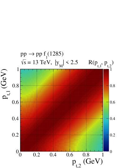
Figure 11: The ratio $R(p_{t,1},p_{t,2})$ (75) for the $pp\to ppf_{1}(1285)$ reaction. The calculation was done for $\sqrt{s}=13$ TeV and with the cut on $|{\rm y_{M}}|<2.5$. No absorption effects were included here.

At the end of this Appendix we give the proof of (70) and (71). For this we study the reaction (69) in the rest system of $f_{1}(k,\epsilon)$ choosing the direction of $q_{1}$ as the $z$ axis. We have then

$$k=\left(\begin{array}[]{c}\sqrt{k^{2}}\\ 0\\ \end{array}\right)\,,\quad q_{1}=\left(\begin{array}[]{c}\frac{1}{2}\sqrt{k^{2}}\\ |\mbox{\boldmath$q_{1}$}|\,\mbox{\boldmath$e_{3}$}\\ \end{array}\right)\,,\quad q_{2}=\left(\begin{array}[]{c}\frac{1}{2}\sqrt{k^{2}}\\ -|\mbox{\boldmath$q_{1}$}|\,\mbox{\boldmath$e_{3}$}\\ \end{array}\right)\,,$$ (82)

$$k^{2}=(q_{1}+q_{2})^{2}=4(m^{2}+|\mbox{\boldmath$q_{1}$}|^{2})\,,$$

$$q_{1}^{0}=q_{2}^{0}=\sqrt{m^{2}+|\mbox{\boldmath$q_{1}$}|^{2}}=\frac{1}{2}\sqrt{k^{2}}\,.$$ (83)

We shall evaluate the ${\cal T}$-matrix elements for (69) in the basis

$$\bra{f_{1}(k,\epsilon^{(M)})}{\cal T}\ket{\mathbb{P}(q_{1},\epsilon_{1}^{(M_{1})}),\mathbb{P}(q_{2},\epsilon_{2}^{(M_{2})})}$$ (84)

where $\epsilon^{(M)}$ and $\epsilon_{1}^{(M_{1})}$, $\epsilon_{2}^{(M_{2})}$ are polarisation vectors and tensors, respectively, corresponding to definite eigenvalues of the angular momentum operator $J_{z}$. In detail we choose for the $f_{1}$

$$\mbox{\boldmath$\epsilon$}^{\,(M=\pm 1)} = \mp\frac{1}{\sqrt{2}}(\mbox{\boldmath$e_{1}$}\pm i\mbox{\boldmath$e_{2}$})\,,$$

$$\mbox{\boldmath$\epsilon$}^{\,(M=0)} = \mbox{\boldmath$e_{3}$}\,.$$ (85)

Here the $J_{z}$ eigenvalues are $M$. For the pomeron (1) we define the four-vectors

$$(\chi_{1}^{\pm\,\mu}) = \mp\frac{1}{\sqrt{2}}\left(\begin{array}[]{c}0\\ \mbox{\boldmath$e_{1}$}\pm i\mbox{\boldmath$e_{2}$}\\ \end{array}\right)\,,$$ (88)

$$(\chi_{1}^{0\,\mu}) = \frac{1}{m}\left(\begin{array}[]{c}|\mbox{\boldmath$q_{1}$}|\\ \mbox{\boldmath$e_{3}$}\,q_{1}^{0}\\ \end{array}\right)$$ (91)

and the polarisation tensors $\epsilon_{1}^{(M_{1})\,\mu\nu}$ ($M_{1}=-2,...,2$) with eigenvalues $M_{1}$ of $J_{z}$ as

$$\epsilon_{1}^{(2)\,\mu\nu} = \chi_{1}^{+\,\mu}\chi_{1}^{+\,\nu}\,,$$

$$\epsilon_{1}^{(1)\,\mu\nu} = \frac{1}{\sqrt{2}}\left(\chi_{1}^{+\,\mu}\chi_{1}^{0\,\nu}+\chi_{1}^{0\,\mu}\chi_{1}^{+\,\nu}\right)\,,$$

$$\epsilon_{1}^{(0)\,\mu\nu} = \frac{1}{\sqrt{6}}\,\chi_{1}^{+\,\mu}\chi_{1}^{-\,\nu}+\sqrt{\frac{2}{3}}\,\chi_{1}^{0\,\mu}\chi_{1}^{0\,\nu}+\frac{1}{\sqrt{6}}\,\chi_{1}^{-\,\mu}\chi_{1}^{+\,\nu}\,,$$

$$\epsilon_{1}^{(-1)\,\mu\nu} = \frac{1}{\sqrt{2}}\left(\chi_{1}^{0\,\mu}\chi_{1}^{-\,\nu}+\chi_{1}^{-\,\mu}\chi_{1}^{0\,\nu}\right)\,,$$

$$\epsilon_{1}^{(-2)\,\mu\nu} = \chi_{1}^{-\,\mu}\chi_{1}^{-\,\nu}\,.$$ (92)

For the pomeron (2) we define the four-vectors

$$(\chi_{2}^{\pm\,\mu}) = \mp\frac{1}{\sqrt{2}}\left(\begin{array}[]{c}0\\ \mbox{\boldmath$e_{1}$}\mp i\mbox{\boldmath$e_{2}$}\\ \end{array}\right)\,,$$ (95)

$$(\chi_{2}^{0\,\mu}) = \frac{1}{m}\left(\begin{array}[]{c}|\mbox{\boldmath$q_{1}$}|\\ -\mbox{\boldmath$e_{3}$}\,q_{1}^{0}\\ \end{array}\right)$$ (98)

and the polarisation tensors $\epsilon_{2}^{(M_{2})\,\mu\nu}$ as in (92) but with $\chi_{1}$ everywhere replaced by $\chi_{2}$. The $\epsilon_{2}^{(M_{2})\,\mu\nu}$ are then the polarisation tensors to the eigenvalues $M_{2}$ of ($-J_{z}$) where $M_{2}\in\{-2,...,2\}$.

Now the stage is set for the evaluation of the ${\cal T}$-matrix elements (84) using either the couplings (52) plus (54) or (61) plus (62). From angular momentum conservation only the elements with

$$M=M_{1}-M_{2}$$ (99)

can be different from zero. The calculations are straightforward but a bit lengthy. We shall only give the results. For this we define two “reduced” amplitudes $\bra{M}\hat{T}^{(2,2)}\ket{M_{1},M_{2}}$ and $\bra{M}\hat{T}^{(4,4)}\ket{M_{1},M_{2}}$; see Table 5.

Table 5: The matrix elements $\bra{M}\hat{T}^{(2,2)}\ket{M_{1},M_{2}}$ and $\bra{M}\hat{T}^{(4,4)}\ket{M_{1},M_{2}}$. Matrix elements not listed are zero.

$M$	$M_{1}$	$M_{2}$	$\bra{M}\hat{T}^{(2,2)}\ket{M_{1},M_{2}}$	$\bra{M}\hat{T}^{(4,4)}\ket{M_{1},M_{2}}$
1	2	1	-1	0
1	1	0	$\frac{1}{\sqrt{6}\,m^{2}}(m^{2}+4|\mbox{\boldmath$q_{1}$}|^{2})$	1
1	0	-1	$\frac{1}{\sqrt{6}\,m^{2}}(m^{2}+4|\mbox{\boldmath$q_{1}$}|^{2})$	1
1	-1	-2	-1	0
-1	1	2	1	0
-1	0	1	$-\frac{1}{\sqrt{6}\,m^{2}}(m^{2}+4|\mbox{\boldmath$q_{1}$}|^{2})$	-1
-1	-1	0	$-\frac{1}{\sqrt{6}\,m^{2}}(m^{2}+4|\mbox{\boldmath$q_{1}$}|^{2})$	-1
-1	-2	-1	1	0

From the Lagrangians (52) plus (54), respectively the vertices (11) plus (12), we obtain for the matrix elements (84)

$$\bra{f_{1}(k,\epsilon^{(M)})}{\cal T}\ket{\mathbb{P}(q_{1},\epsilon_{1}^{(M_{1})}),\mathbb{P}(q_{2},\epsilon_{2}^{(M_{2})})} = g^{\prime}_{\mathbb{P}\mathbb{P}f_{1}}\,\frac{k^{2}\,\sqrt{2}\,|\mbox{\boldmath$q_{1}$}|^{2}}{M_{0}^{2}\,m}\,\bra{M}\hat{T}^{(2,2)}\ket{M_{1},M_{2}}$$ (100)

$$+ g^{\prime\prime}_{\mathbb{P}\mathbb{P}f_{1}}\,\frac{(k^{2})^{2}\,|\mbox{\boldmath$q_{1}$}|^{4}}{\sqrt{3}\,M_{0}^{4}\,m^{3}}\,\bra{M}\hat{T}^{(4,4)}\ket{M_{1},M_{2}}\,.\qquad\quad$$

Note that the $(l,S)=(2,2)$ coupling gives an amplitude proportional to $|\mbox{\boldmath$q_{1}$}|^{2}$, the $(l,S)=(4,4)$ term an amplitude proportional to $|\mbox{\boldmath$q_{1}$}|^{4}$, as it should be for these values of the orbital angular momentum $l$.

Now we consider the Lagrangians (61) plus (62) giving the vertices (66) and (67), respectively. Here we get for the matrix elements (84)

$$\bra{f_{1}(k,\epsilon^{(M)})}{\cal T}\ket{\mathbb{P}(q_{1},\epsilon_{1}^{(M_{1})}),\mathbb{P}(q_{2},\epsilon_{2}^{(M_{2})})}$$

$$\qquad\qquad\qquad=-\left(\varkappa^{\prime}+\varkappa^{\prime\prime}\frac{k^{2}-2m^{2}}{2}\right)\,\frac{\sqrt{2}\,|\mbox{\boldmath$q_{1}$}|^{2}}{m}\,\bra{M}\hat{T}^{(2,2)}\ket{M_{1},M_{2}}$$

$$\qquad\qquad\qquad\quad\,+\varkappa^{\prime\prime}\,\frac{2k^{2}\,|\mbox{\boldmath$q_{1}$}|^{4}}{\sqrt{3}\,m^{3}}\,\bra{M}\hat{T}^{(4,4)}\ket{M_{1},M_{2}}\,.$$ (101)

Equating the expressions (100) and (101) we arrive at the relations (71) which are, therefore, proved.

Appendix C The $f_{1}$ mixing angle and relations between the $\mathbb{P}\mathbb{P}f_{1}(1285)$ and $\mathbb{P}\mathbb{P}f_{1}(1420)$ coupling constants

The different magnitude of the coupling constants for the $\mathbb{P}\mathbb{P}f_{1}(1285)$ and $\mathbb{P}\mathbb{P}f_{1}(1420)$ interactions can be expected to be related to the internal structure of the mesons.

A commonly used model is given by

$$f_{1}(1285) = \cos\phi_{f}\frac{u\bar{u}+d\bar{d}}{\sqrt{2}}-\sin\phi_{f}\;s\bar{s}\,,$$

$$f_{1}(1420) = \sin\phi_{f}\frac{u\bar{u}+d\bar{d}}{\sqrt{2}}+\cos\phi_{f}\;s\bar{s}\,,$$ (102)

with a mixing angle $\phi_{f}$ parametrising the deviation from “ideal” mixing ($\phi_{f}=0^{\circ}$), where the heavier $f_{1}$ meson would be purely $s\bar{s}$.

Ideal mixing is often assumed as a first approximation to account for the fact that $f_{1}(1420)$ decays dominantly into $K\bar{K}\pi$ Tanabashi:2018oca . Radiative processes, however, indicate a deviation from ideal mixing of about $\phi_{f}\simeq+20^{\circ}$ Leutgeb:2019gbz which is consistent with the LHCb result Aaij:2013rja of $\phi_{f}=\pm(24\pm 3)^{\circ}$ and with other results pointing to a range of $+(20\cdots 30)^{\circ}$ Dudek:2011tt ; Cheng:2011pb .

In the chirally symmetric Sakai-Sugimoto model the $\mathbb{P}\mathbb{P}f_{1}$ couplings come exclusively from the axial-gravitational anomaly which involves only the flavour-singlet combination $(u\bar{u}+d\bar{d}+s\bar{s})/\sqrt{3}$. The assumption that this also holds true in real QCD would give

$$\frac{g^{\prime}_{\mathbb{P}\mathbb{P}f_{1}(1420)}}{g^{\prime}_{\mathbb{P}\mathbb{P}f_{1}(1285)}}=\frac{\sqrt{2}\sin\phi_{f}+\cos\phi_{f}}{\sqrt{2}\cos\phi_{f}-\sin\phi_{f}}\,.$$ (103)

and likewise for the couplings $g^{\prime\prime}$, $\varkappa^{\prime}$, and $\varkappa^{\prime\prime}$. Ideal mixing thus corresponds to

$$\frac{g^{\prime}_{\mathbb{P}\mathbb{P}f_{1}(1420)}}{g^{\prime}_{\mathbb{P}\mathbb{P}f_{1}(1285)}}\Big{|}_{\phi_{f}=0^{\circ}}=\frac{1}{\sqrt{2}}\,,$$ (104)

while $\phi_{f}\simeq+20^{\circ}$ gives ratios larger than unity,

$$\frac{g^{\prime}_{\mathbb{P}\mathbb{P}f_{1}(1420)}}{g^{\prime}_{\mathbb{P}\mathbb{P}f_{1}(1285)}}\Big{|}_{\phi_{f}\simeq+20^{\circ}}\simeq 1.44\,.$$ (105)

But due to mass effects, the relation (103) is expected to be only qualitatively correct. And, indeed, we have seen in (41) that the WA102 data violate (104) or (105) by a factor of about 1.5 or 3, respectively. If we blame this violation on the subleading reggeon exchanges we get an indication that the true $\mathbb{P}\mathbb{P}f_{1}$ couplings could differ from those given in (27) and (35) by a factor of this magnitude.

However, the assumption that the pomeron couples only to the above flavour singlet $q\bar{q}$ combination is questionable since it is based on the assumption of exact flavour SU(3) symmetry. In fact, the SU(3) flavour symmetry is known to be violated, also for diffractive processes. For instance, the pomeron coupling to pions is different (larger) than that for kaons (see, e.g., Donnachie:2002en ). The same is true for the coupling of the pomeron to $\rho^{0}$, $\omega$, and $\phi$ vector mesons; see Lebiedowicz:2014bea ; Lebiedowicz:2019boz .

Appendix D Discussion of subleading exchanges

In the main text we have assumed that the pomeron-pomeron fusion is the dominant reaction mechanism at the top WA102 energy $\sqrt{s}=29.1$ GeV Barberis:1998by . In fact the WA102 Collaboration measured $f_{1}(1285)$ and $f_{1}(1420)$ also at the significantly lower energy $\sqrt{s}=12.7$ GeV.

For a complete theoretical discussion of all results of the WA102 experiment we should consider also the lower energy and include subleading reggeon-exchange contributions to $f_{1}$ CEP. We list here the possible fusion reactions leading to an $f_{1}$ meson and involving such reggeons:

$$\mathbb{P}f_{2\mathbb{R}}+f_{2\mathbb{R}}\mathbb{P}\to f_{1}\,,$$ (106)

$$f_{2\mathbb{R}}f_{2\mathbb{R}}\to f_{1}\,,$$ (107)

$$a_{2\mathbb{R}}a_{2\mathbb{R}}\to f_{1}\,,$$ (108)

$$\omega_{\mathbb{R}}\omega_{\mathbb{R}}\to f_{1}\,,$$ (109)

$$\rho_{\mathbb{R}}\rho_{\mathbb{R}}\to f_{1}\,,$$ (110)

$$\phi_{\mathbb{R}}\phi_{\mathbb{R}}\to f_{1}\,.$$ (111)

Let us now discuss the effective couplings for these processes, taking as a model the results of Appendix A; see (49)–(54). Following Ewerz:2013kda the $f_{2\mathbb{R}}$ and $a_{2\mathbb{R}}$ reggeons will be treated as effective second rank symmetric traceless tensors, the $\omega_{\mathbb{R}}$, $\rho_{\mathbb{R}}$, and $\phi_{\mathbb{R}}$ as effective vectors.

Our coupling Lagrangians for (107) and (108) are then as in (52) and (54) but with the replacements

$$g^{\prime}_{\mathbb{P}\mathbb{P}f_{1}}\to g^{\prime}_{f_{2\mathbb{R}}f_{2\mathbb{R}}f_{1}}\,,\quad g^{\prime\prime}_{\mathbb{P}\mathbb{P}f_{1}}\to g^{\prime\prime}_{f_{2\mathbb{R}}f_{2\mathbb{R}}f_{1}}\,,$$ (112)

and

$$g^{\prime}_{\mathbb{P}\mathbb{P}f_{1}}\to g^{\prime}_{a_{2\mathbb{R}}a_{2\mathbb{R}}f_{1}}\,,\quad g^{\prime\prime}_{\mathbb{P}\mathbb{P}f_{1}}\to g^{\prime\prime}_{a_{2\mathbb{R}}a_{2\mathbb{R}}f_{1}}\,,$$ (113)

respectively. All these couplings must be real. For the process (106) there are more coupling possibilities than the analogs of (52) and (54), since $\mathbb{P}$ and $f_{2\mathbb{R}}$ are distinct. Indeed, using the methods of Appendix A of Lebiedowicz:2013ika , we find here six independent couplings.

For the process (109) we can rely on the general analysis of two real vector particles giving an $f_{1}$ with $J^{P}=1^{+}$ in Appendix B of Lebiedowicz:2013ika . From Table 8 there we find that there is only one possible coupling, $(l,S)=(2,2)$, for this on-shell process. A convenient coupling Lagrangian is easily written down

$${\cal L}^{\prime}_{\omega_{\mathbb{R}}\omega_{\mathbb{R}}f_{1}}(x)=\frac{1}{M_{0}^{4}}g_{\omega_{\mathbb{R}}\omega_{\mathbb{R}}f_{1}}\Big{(}\omega_{\mathbb{R}\,\kappa\lambda}(x)\stackrel{{\scriptstyle\leftrightarrow}}{{\partial}}_{\!\mu}\stackrel{{\scriptstyle\leftrightarrow}}{{\partial}}_{\!\nu}\omega_{\mathbb{R}\,\rho\sigma}(x)\Big{)}\Big{(}\partial_{\alpha}U_{\beta}(x)-\partial_{\beta}U_{\alpha}(x)\Big{)}g^{\kappa\rho}g^{\mu\sigma}\varepsilon^{\lambda\nu\alpha\beta},$$

(114)

where

$$\omega_{\mathbb{R}\,\kappa\lambda}(x)=\partial_{\kappa}\omega_{\mathbb{R}\,\lambda}(x)-\partial_{\lambda}\omega_{\mathbb{R}\,\kappa}(x)$$ (115)

and $g_{\omega_{\mathbb{R}}\omega_{\mathbb{R}}f_{1}}$ is a dimensionless coupling constant. Similar coupling ansätze apply to the processes (110) and (111).

The vertex following from (114) reads as follows:
      

$$i\Gamma_{\mu\nu\alpha}^{(\omega_{\mathbb{R}}\omega_{\mathbb{R}}f_{1})}(q_{1},q_{2})\mid_{\rm{bare}} = \frac{2g_{\omega_{\mathbb{R}}\omega_{\mathbb{R}}f_{1}}}{M_{0}^{4}}\Bigl{[}(q_{1}-q_{2})^{\rho}(q_{1}-q_{2})^{\sigma}\varepsilon_{\lambda\sigma\alpha\beta}\,k^{\beta}$$ (116)

$$\times(q_{1\kappa}\,\delta^{\lambda}_{\;\;\mu}-q_{1}^{\lambda}\,g_{\kappa\mu})(q_{2}^{\kappa}\,g_{\rho\nu}-q_{2\rho}\,\delta^{\kappa}_{\;\;\nu})+(q_{1}\leftrightarrow q_{2},\mu\leftrightarrow\nu)\Bigr{]}.\qquad\;\;$$

This vertex function satisfies the relations

$$\Gamma_{\mu\nu\alpha}^{(\omega_{\mathbb{R}}\omega_{\mathbb{R}}f_{1})}(q_{1},q_{2})=\Gamma_{\nu\mu\alpha}^{(\omega_{\mathbb{R}}\omega_{\mathbb{R}}f_{1})}(q_{2},q_{1})\,,$$

$$\Gamma_{\mu\nu\alpha}^{(\omega_{\mathbb{R}}\omega_{\mathbb{R}}f_{1})}(q_{1},q_{2})\,q_{1}^{\mu}=0\,,$$

$$\Gamma_{\mu\nu\alpha}^{(\omega_{\mathbb{R}}\omega_{\mathbb{R}}f_{1})}(q_{1},q_{2})\,q_{2}^{\nu}=0\,,$$

$$\Gamma_{\mu\nu\alpha}^{(\omega_{\mathbb{R}}\omega_{\mathbb{R}}f_{1})}(q_{1},q_{2})\,(q_{1}+q_{2})^{\alpha}=0\,.$$ (117)

We shall use in the following the coupling (114) and the vertex function (116) for $\omega$ reggeons as well as $\omega$ mesons.

As for the case of the $\mathbb{P}\mathbb{P}f_{1}$ coupling we find it useful to consider the analog of the reaction (69) here, the fusion of two real $\omega$ mesons giving an $f_{1}$ state

$$\omega(q_{1},\epsilon_{1}^{(M_{1})})+\omega(q_{2},\epsilon_{2}^{(M_{2})})\to f_{1}(k,\epsilon^{(M)})\,.$$ (118)

For our purpose we consider fictitious $\omega$ mesons of arbitrary mass $m\geqslant 0$ and a fictitious $f_{1}$ of mass $\sqrt{k^{2}}\geqslant 2m$. We shall work again in the rest system of the $f_{1}$ and choose the kinematics as in (83). The polarisation vectors $\epsilon^{(M)}$ ($M=\pm 1,0$) for the $f_{1}$ are taken as in (85). The polarisation vectors for the $\omega$ mesons are taken as follows

$$\epsilon_{1}^{(M_{1})}=\chi_{1}^{(M_{1})}\,,\quad\epsilon_{2}^{(M_{2})}=\chi_{2}^{(M_{2})}$$ (119)

with $M_{1},M_{2}\in\{\pm 1,0\}$ and $\chi_{1}^{(M_{1})}$ and $\chi_{2}^{(M_{2})}$ as in (91) and (98), respectively.

After a straightforward calculation we find

$$\bra{f_{1}(k,\epsilon^{(M)})}{\cal T}\ket{\omega(q_{1},\epsilon_{1}^{(M_{1})}),\omega(q_{2},\epsilon_{2}^{(M_{2})})}=-\frac{4g_{\omega_{\mathbb{R}}\omega_{\mathbb{R}}f_{1}}}{M_{0}^{4}}\,k^{2}\,m\,|\mbox{\boldmath$q_{1}$}|^{2}$$

$$\qquad\times\left\{\delta_{M,1}\left[\delta_{M_{1},0}\,\delta_{M_{2},-1}+\delta_{M_{1},1}\,\delta_{M_{2},0}\right]-\delta_{M,-1}\left[\delta_{M_{1},0}\,\delta_{M_{2},1}+\delta_{M_{1},-1}\,\delta_{M_{2},0}\right]\right\}\,.\quad$$ (120)

Note that the amplitude (120) is proportional to $|\mbox{\boldmath$q_{1}$}|^{2}$ as it should be since it is derived from the $(l,S)=(2,2)$ coupling (114). Furthermore, the amplitude (120) vanishes for $m=0$ as it must be due to the Landau-Yang theorem Landau:1948kw ; Yang:1950rg . Indeed, we can consider the production of an $f_{1}$ meson by two virtual photons of mass squared $q^{2}\geqslant 0$. For this we use the standard vector-meson-dominance (VMD) ansatz for the coupling of the photons to the $\omega$ mesons [see, e.g., (3.23) of Ewerz:2013kda ], which then fuse to give the $f_{1}$. In this case we get for the amplitude the same expression as in (120) with $m$ replaced by $\sqrt{q^{2}}$ and multiplied with the appropriate VMD factor times a vertex form factor $F(q^{2},q^{2},k^{2})$

$$\left(e\frac{m_{\omega}^{2}}{\gamma_{\omega}}\Delta_{T}^{(\omega)}(q^{2})\right)^{2}F(q^{2},q^{2},k^{2})\,,$$ (121)

where $\Delta_{T}^{(\omega)}(q^{2})$ is the transverse part of the $\omega$ meson propagator [cf. (3.2)–(3.4) of Ewerz:2013kda ]. All gauge invariance relations for these amplitudes are satisfied due to (117) and the amplitudes vanish for $q^{2}\to 0$ in accord with the Landau-Yang theorem.

A different ansatz for the $\omega_{\mathbb{R}}\omega_{\mathbb{R}}f_{1}$ coupling is obtained in the holographic approach Domokos:2009cq :

$${\cal L^{\prime}}^{\,{\rm CS}}_{\omega_{\mathbb{R}}\omega_{\mathbb{R}}f_{1}}(x)=\varkappa_{\omega}\,\varepsilon^{\alpha\beta\gamma\delta}\,U_{\alpha}(x)\,\omega_{\mathbb{R}\beta}(x)\,\partial_{\gamma}\,\omega_{\mathbb{R}\delta}(x)\,,$$ (122)

$$i\Gamma_{\mu\nu\alpha}^{{\rm CS}\,(\omega_{\mathbb{R}}\omega_{\mathbb{R}}f_{1})}(q_{1},q_{2})\mid_{\rm{bare}}=\varkappa_{\omega}\,\varepsilon_{\alpha\mu\nu\rho}\,(q_{1}-q_{2})^{\rho}\,$$ (123)

with $\varkappa_{\omega}$ a dimensionless parameter. For the vertex function (123) we find the relations

$$\Gamma_{\mu\nu\alpha}^{{\rm CS}\,(\omega_{\mathbb{R}}\omega_{\mathbb{R}}f_{1})}(q_{1},q_{2})=\Gamma_{\nu\mu\alpha}^{{\rm CS}\,(\omega_{\mathbb{R}}\omega_{\mathbb{R}}f_{1})}(q_{2},q_{1})\,;$$ (124)

$$\Gamma_{\mu\nu\alpha}^{{\rm CS}\,(\omega_{\mathbb{R}}\omega_{\mathbb{R}}f_{1})}(q_{1},q_{2})\,q_{1}^{\mu}=i\varkappa_{\omega}\,\varepsilon_{\alpha\mu\nu\rho}\,q_{1}^{\mu}q_{2}^{\rho}\neq 0\,,$$

$$\Gamma_{\mu\nu\alpha}^{{\rm CS}\,(\omega_{\mathbb{R}}\omega_{\mathbb{R}}f_{1})}(q_{1},q_{2})\,q_{2}^{\nu}=-i\varkappa_{\omega}\,\varepsilon_{\alpha\mu\nu\rho}\,q_{1}^{\rho}q_{2}^{\nu}\neq 0\,;$$ (125)

$$\Gamma_{\mu\nu\alpha}^{{\rm CS}\,(\omega_{\mathbb{R}}\omega_{\mathbb{R}}f_{1})}(q_{1},q_{2})\,(q_{1}+q_{2})^{\alpha}=-i\varkappa_{\omega}\,\varepsilon_{\alpha\mu\nu\rho}\,(q_{1}+q_{2})^{\alpha}(q_{1}-q_{2})^{\rho}\neq 0\,.$$ (126)

For the process (118) we find here

$$\bra{f_{1}(k,\epsilon^{(M)})}{\cal T}\ket{\omega(q_{1},\epsilon_{1}^{(M_{1})}),\omega(q_{2},\epsilon_{2}^{(M_{2})})}=\varkappa_{\omega}\frac{2|\mbox{\boldmath$q_{1}$}|^{2}}{m}$$

$$\qquad\times\left\{\delta_{M,1}\left[\delta_{M_{1},0}\,\delta_{M_{2},-1}+\delta_{M_{1},1}\,\delta_{M_{2},0}\right]-\delta_{M,-1}\left[\delta_{M_{1},0}\,\delta_{M_{2},1}+\delta_{M_{1},-1}\,\delta_{M_{2},0}\right]\right\}\,.\quad$$ (127)

With constant $\varkappa_{\omega}$, these amplitudes diverge for $m\to 0$. Here we cannot use the usual VMD relations to relate these amplitudes to the ones for the fusion of two virtual or real photons giving an $f_{1}$ meson. Because of (125) the corresponding amplitudes for $\gamma^{*}\gamma^{*}\to f_{1}$ would not satisfy the necessary gauge invariance relations.

Vector-meson dominance is, in fact, realized in holographic QCD (for an extensive discussion in the Sakai-Sugimoto model see Sakai:2005yt ). The coupling to virtual or real photons involves bulk-to-boundary propagators which correspond to sums over an infinite tower of massive vector mesons. In place of the constant $\varkappa_{\omega}$ one obtains an asymmetric transition form factor that does satisfy the Landau-Yang theorem and which has been studied in Leutgeb:2019gbz , where good agreement with available data from the L3 experiment Achard:2001uu ; Achard:2007hm on single-virtual $\gamma\gamma^{*}\to f_{1}$ has been found.

Clearly the inclusion of all these subleading exchanges (106)–(111) would introduce many new coupling parameters and form factors and would make a meaningful analysis of the WA102 data practically impossible. However, for the analysis of data from the COMPASS experiment, which operates in the same energy range as previously the WA102 experiment, it could be very worthwhile to study all the above subleading exchanges in detail. In addition one also has to keep in mind that there should be a smooth transition from reggeon to particle exchanges when going to very low energies. Clearly, all these topics deserve careful analyses, but they go beyond the scope of the present paper.

Here we shall only discuss some rough estimates of subleading contributions at the WA102 energy of $\sqrt{s}=29.1$ GeV.

At the relatively low energies of the WA102 experiment the subleading reggeon exchanges are not excluded a priori. Among those, the $\omega\omega\to f_{1}$ and $\rho^{0}\rho^{0}\to f_{1}$ exchanges are the most probable ones. We know how the $\omega$ and $\rho^{0}$ couple to nucleons. However, the coupling of $\omega\omega\to f_{1}$ and $\rho^{0}\rho^{0}\to f_{1}$ is less known. Future experiments at HADES and PANDA will provide new information there. The $\rho^{0}\rho^{0}\to f_{1}$ coupling constant can be obtained from the decays: $f_{1}\to\rho^{0}\gamma$ and/or $f_{1}\to\pi^{+}\pi^{-}\pi^{+}\pi^{-}$. This issue will be discussed elsewhere. The uncertainties related to form factors preclude, however, strict predictions. Fortunately, the following (almost model independent) observation explains the situation. It seems rather obvious that the reggeized-vector-meson-exchange or reggeon-reggeon-exchange contributions cannot exceed the experimental data of the WA102 Collaboration Barberis:1998by . According to our estimates we find, using subleading exchanges only, that they allow a description of the $\sqrt{s}=12.7$ GeV data (see Table 1) but then one misses the data for $\sqrt{s}=29.1$ GeV by a factor of at least 5. This is due to the energy dependence of the subleading contributions. This means that the dominant contribution at $\sqrt{s}=29.1$ GeV is most probably related to the double-pomeron-exchange contribution considered in our paper.

To make this statement quantitative we proceed as follows. Let ${\cal M}$ be the amplitude for the $\mathbb{P}\mathbb{P}\to f_{1}$ fusion as calculated in the present paper with which we could fit the WA102 data for $\sqrt{s}=29.1$ GeV. We assume now that the true $\mathbb{P}\mathbb{P}\to f_{1}$ fusion amplitude is $x{\cal M}$ ($x>0$) and that the reggeon amplitude is similar in structure to the pomeron amplitude and given by $y{\cal M}$. We must have then, precluding a complete sign change of the amplitudes,

$$x+y=1\,.$$ (128)

From the above estimates of the reggeon contributions alone we get

$$|y|^{2}\leqslant 0.20\,.$$ (129)

For maximal constructive interference of pomeron and reggeon contributions we get

$$\begin{split}&y\leqslant\sqrt{0.20}=0.45\,,\\ &x=1-y\geqslant 0.55\,.\end{split}$$ (130)

For destructive interference we would get $x>1$. The result (130) is the basis for the estimate that the true $\mathbb{P}\mathbb{P}f_{1}$ couplings may be up to a factor of 2 smaller than the ones obtained in our present paper from the comparison of the WA102 data at $\sqrt{s}=29.1$ GeV to our theory neglecting the reggeons.

Appendix E The $\phi_{pp}$ distributions for CEP of $f_{1}$- and $\eta$-type mesons at $\phi_{pp}=0$ and $\pi$

Here we discuss general properties of the $\phi_{pp}$ distributions for CEP of $f_{1}$ mesons (1) and for the analogous reaction with $\eta$-type mesons

$$p(p_{a},\lambda_{a})+p(p_{b},\lambda_{b})\to p(p_{1},\lambda_{1})+\eta(k)+p(p_{2},\lambda_{2})\,.$$ (131)

Recall that $\phi_{pp}$ is the azimuthal angle between the transverse momenta of the two outgoing protons in the overall c.m. system (Fig. 12). For the following arguments we work in this c.m. system.

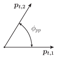
Figure 12: Definition of the angle $\phi_{pp}$ ($0\leqslant\phi_{pp}\leqslant\pi$).

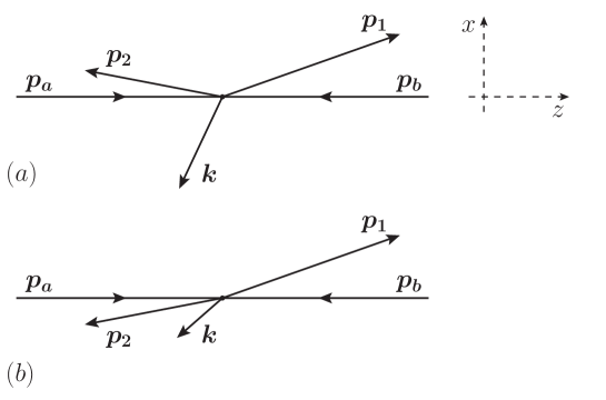
Figure 13: Sketch of CEP reactions with (a) $\phi_{pp}=0$ and (b) $\phi_{pp}=\pi$ and definition of the $x$ and $z$ axes.

For $\phi_{pp}=0$ and $\pi$ the reaction (131) is planar (Fig. 13). We choose the reaction plane as the $xz$ plane of our coordinate system. Note that this plane is a symmetry plane for our reaction and we shall exploit this in the following.

In (1) and (131) we have written our reactions in terms of protons with definite helicities $\lambda_{a},\lambda_{b},\lambda_{1},\lambda_{2}\in\{1/2,-1/2\}$. Here we shall use protons with spin $\tilde{\lambda}=\pm 1/2$ in the $y$ direction, orthogonal to the reaction plane. We have

$$\ket{p(\mbox{\boldmath$p$},\tilde{\lambda})}_{y}=\frac{1}{\sqrt{2}}\left(\ket{p(\mbox{\boldmath$p$},1/2)}+i2\tilde{\lambda}\ket{p(\mbox{\boldmath$p$},-1/2)}\right)\,,$$

$$\tilde{\lambda}=\pm 1/2\,,\quad\mbox{\boldmath$p$}=\mbox{\boldmath$p_{a}$},\mbox{\boldmath$p_{b}$},\mbox{\boldmath$p_{1}$},\mbox{\boldmath$p_{2}$}\,.$$ (132)

Now we consider a reflection $S$ on the $xz$ plane. $S$ can be written as a parity transformation, $P$, times a rotation $R_{2}(\pi)$ by $\pi$ around the $y$ axis

$$S=R_{2}(\pi)\,P\,.$$ (133)

For the proton states (132) this gives

$$U(S)\ket{p(\mbox{\boldmath$p$},\tilde{\lambda})}_{y}=e^{i\pi\tilde{\lambda}}\ket{p(\mbox{\boldmath$p$},\tilde{\lambda})}_{y}\,.$$ (134)

Assumption:

Now we assume that at high energies there is $s$-channel helicity conservation of the protons in (131) and, more strongly, helicity independence. That is, we assume

$$\bra{p(p_{1},\lambda_{1}),p(p_{2},\lambda_{2}),\eta(k)}{\cal T}\ket{p(p_{a},\lambda_{a}),p(p_{b},\lambda_{b})}\propto\delta_{\lambda_{1}\lambda_{a}}\,\delta_{\lambda_{2}\lambda_{b}}\,.$$ (135)

In our calculations for CEP reactions of $f_{1}$ we always used this high-energy approximation for the protons. Transforming to the states (132) we also get there

$$\bra{p(p_{1},\tilde{\lambda}_{1}),p(p_{2},\tilde{\lambda}_{2}),\eta(k)}{\cal T}\ket{p(p_{a},\tilde{\lambda}_{a}),p(p_{b},\tilde{\lambda}_{b})}_{y}\propto\delta_{\tilde{\lambda}_{1}\tilde{\lambda}_{a}}\,\delta_{\tilde{\lambda}_{2}\tilde{\lambda}_{b}}\,.$$ (136)

The next step is to apply to the ${\cal T}$-matrix element (136) a reflection transformation $S$ (133). With (134) and (136) we get for the pseudoscalar $\eta$

$$\bra{p(p_{1},\tilde{\lambda}_{1}),p(p_{2},\tilde{\lambda}_{2}),\eta(k)}{\cal T}\ket{p(p_{a},\tilde{\lambda}_{a}),p(p_{b},\tilde{\lambda}_{b})}_{y}$$

$$=(-1)\exp\left[i\pi\left(\tilde{\lambda}_{a}-\tilde{\lambda}_{1}+\tilde{\lambda}_{b}-\tilde{\lambda}_{2}\right)\right]\bra{p(p_{1},\tilde{\lambda}_{1}),p(p_{2},\tilde{\lambda}_{2}),\eta(k)}{\cal T}\ket{p(p_{a},\tilde{\lambda}_{a}),p(p_{b},\tilde{\lambda}_{b})}_{y}$$

$$=0\,.$$ (137)

This proves that under the above assumption the distribution in $\phi_{pp}$ must vanish for $\phi_{pp}=0$ and $\pi$ in CEP of $\eta$-type mesons.

The $\phi_{pp}$ distributions in CEP of the $\eta$ of mass 548 MeV and $\eta^{\prime}(958)$ were studied in the WA102 experiment Barberis:1998ax and, using our theoretical framework, in Lebiedowicz:2013ika ; see Fig. 14 there. The experimental distributions vanish for $\phi_{pp}=0$, but at $\phi_{pp}=\pi$ a small residual different from zero is visible. According to our results this must be due to contributions violating our assumptions concerning the helicities.

Finally we return to $f_{1}$ production (1). For an $f_{1}$ meson with $J^{P}=1^{+}$ we can use the Wigner basis with the $f_{1}$ polarisation vectors $\mbox{\boldmath$e_{x}$},\mbox{\boldmath$e_{y}$},\mbox{\boldmath$e_{z}$}$. Under the reflection $S$ we have the following transformation properties

$$U(S)\ket{f_{1}(\mbox{\boldmath$k$},\mbox{\boldmath$e_{x}$})}=-\ket{f_{1}(\mbox{\boldmath$k$},\mbox{\boldmath$e_{x}$})}\,,$$

$$U(S)\ket{f_{1}(\mbox{\boldmath$k$},\mbox{\boldmath$e_{y}$})}=\quad\ket{f_{1}(\mbox{\boldmath$k$},\mbox{\boldmath$e_{y}$})}\,,$$

$$U(S)\ket{f_{1}(\mbox{\boldmath$k$},\mbox{\boldmath$e_{z}$})}=-\ket{f_{1}(\mbox{\boldmath$k$},\mbox{\boldmath$e_{z}$})}\,.$$ (138)

Using now the same argumentation as for $\eta$-type mesons above we conclude that for $\phi_{pp}=0$ and $\pi$ the produced $f_{1}$ must have the polarisation in the $y$ direction, that is, transverse to the reaction plane.

To summarize: in this appendix we have shown the following theorem. Assuming $s$-channel helicity conservation and helicity independence for CEP of $\eta$- and $f_{1}$-type mesons the $\phi_{pp}$ distributions must vanish for $\phi_{pp}=0$ and $\pi$ for the $\eta$ case and the $f_{1}$ must be polarised transversely to the reaction plane for these $\phi_{pp}$ values.

- (1) D. Barberis et al., (WA102 Collaboration), A study of the centrally produced channel in interactions at 450 GeV/, Phys. Lett. B413 (1997) 217, arXiv:9707021 [hep-ex].
- (2) D. Barberis et al., (WA102 Collaboration), A study of the channel produced centrally in interactions at 450 GeV/, Phys. Lett. B413 (1997) 225, arXiv:hep-ex/9707022 [hep-ex].
- (3) D. Barberis et al., (WA102 Collaboration), A measurement of the branching fractions of the and produced in central interactions at 450 GeV/, Phys. Lett. B440 (1998) 225, arXiv:hep-ex/9810003 [hep-ex].
- (4) M. Tanabashi et al., (Particle Data Group), Review of Particle Physics, Phys. Rev. D98 no. 3, (2018) 030001.
- (5) D. Barberis et al., (WA102 Collaboration), A spin analysis of the channels produced in central interactions at 450 GeV/, Phys.Lett. B471 (2000) 440, arXiv:9912005 [hep-ex].
- (6) F. E. Close and A. Kirk, Glueball- filter in central hadron production, Phys.Lett. B397 (1997) 333, arXiv:hep-ph/9701222 [hep-ph].
- (7) A. A. Osipov, A. A. Pivovarov, and M. K. Volkov, Decay rates and in the Nambu–Jona-Lasinio model, Phys. Rev. D98 no. 1, (2018) 014037, arXiv:1805.10907 [hep-ph].
- (8) M. Birkel and H. Fritzsch, Nucleon spin and the mixing of axial vector mesons, Phys. Rev. D53 (1996) 6195, arXiv:hep-ph/9511424 [hep-ph].
- (9) P. G. Moreira and M. L. L. da Silva, Investigating the glue content of , Nuclear Physics A 992 (2019) 121641, arXiv:1712.04783 [hep-ph].
- (10) F. E. Close and A. Kirk, Implications of the Glueball- filter on the nonet, Z. Phys. C 76 (1997) 469, arXiv:hep-ph/9706543.
- (11) D.-M. Li, H. Yu, and Q.-X. Shen, Is the Partner of in the Nonet?, Chin. Phys. Lett. 17 (2000) 558, arXiv:hep-ph/0001011.
- (12) V. Debastiani, F. Aceti, W.-H. Liang, and E. Oset, Revising the resonance, Phys. Rev. D 95 no. 3, (2017) 034015, arXiv:1611.05383 [hep-ph].
- (13) X.-Y. Wang, J. He, Q. Wang, and H. Xu, Productions of in pion and kaon induced reactions, Phys. Rev. D 99 no. 1, (2019) 014020, arXiv:1810.04096 [hep-ph].
- (14) W.-H. Liang and E. Oset, Testing the origin of the “” with the reaction, Eur. Phys. J. C 80 no. 5, (2020) 407, arXiv:2001.03299 [hep-ph].
- (15) C. Ewerz, M. Maniatis, and O. Nachtmann, A Model for Soft High-Energy Scattering: Tensor Pomeron and Vector Odderon, Annals Phys. 342 (2014) 31, arXiv:1309.3478 [hep-ph].
- (16) O. Nachtmann, Considerations concerning diffraction scattering in quantum chromodynamics, Annals Phys. 209 (1991) 436.
- (17) R. C. Brower, J. Polchinski, M. J. Strassler, and C.-I. Tan, The Pomeron and gauge/string duality, JHEP 12 (2007) 005, arXiv:hep-th/0603115.
- (18) S. K. Domokos, J. A. Harvey, and N. Mann, The Pomeron contribution to and scattering in AdS/QCD, Phys. Rev. D 80 (2009) 126015, arXiv:0907.1084 [hep-ph].
- (19) N. Anderson, S. K. Domokos, J. A. Harvey, and N. Mann, Central production of and via double Pomeron exchange in the Sakai-Sugimoto model, Phys. Rev. D90 no. 8, (2014) 086010, arXiv:1406.7010 [hep-ph].
- (20) A. Ballon-Bayona, R. Carcassés Quevedo, M. S. Costa, and M. Djurić, Soft Pomeron in Holographic QCD, Phys. Rev. D 93 (2016) 035005, arXiv:1508.00008 [hep-ph].
- (21) I. Iatrakis, A. Ramamurti, and E. Shuryak, Pomeron Interactions from the Einstein-Hilbert Action, Phys. Rev. D 94 no. 4, (2016) 045005, arXiv:1602.05014 [hep-ph].
- (22) N. Anderson, S. Domokos, and N. Mann, Central production of via double Pomeron exchange and double Reggeon exchange in the Sakai-Sugimoto model, Phys. Rev. D 96 no. 4, (2017) 046002, arXiv:1612.07457 [hep-ph].
- (23) L. Adamczyk et al., (STAR Collaboration), Single spin asymmetry in polarized proton-proton elastic scattering at GeV, Phys. Lett. B719 (2013) 62, arXiv:1206.1928 [nucl-ex].
- (24) C. Ewerz, P. Lebiedowicz, O. Nachtmann, and A. Szczurek, Helicity in Proton-Proton Elastic Scattering and the Spin Structure of the Pomeron, Phys. Lett. B763 (2016) 382, arXiv:1606.08067 [hep-ph].
- (25) D. Britzger, C. Ewerz, S. Glazov, O. Nachtmann, and S. Schmitt, The Tensor Pomeron and Low- Deep Inelastic Scattering, Phys. Rev. D100 no. 11, (2019) 114007, arXiv:1901.08524 [hep-ph].
- (26) P. Lebiedowicz, O. Nachtmann, and A. Szczurek, Exclusive central diffractive production of scalar and pseudoscalar mesons; tensorial vs. vectorial pomeron, Annals Phys. 344 (2014) 301, arXiv:1309.3913 [hep-ph].
- (27) P. Lebiedowicz, O. Nachtmann, and A. Szczurek, and Drell-Söding contributions to central exclusive production of pairs in proton-proton collisions at high energies, Phys. Rev. D91 (2015) 074023, arXiv:1412.3677 [hep-ph].
- (28) P. Lebiedowicz, O. Nachtmann, and A. Szczurek, Central exclusive diffractive production of the continuum, scalar, and tensor resonances in and scattering within the tensor Pomeron approach, Phys. Rev. D93 (2016) 054015, arXiv:1601.04537 [hep-ph].
- (29) P. Lebiedowicz, O. Nachtmann, and A. Szczurek, Central production of in collisions with single proton diffractive dissociation at the LHC, Phys. Rev. D95 no. 3, (2017) 034036, arXiv:1612.06294 [hep-ph].
- (30) P. Lebiedowicz, O. Nachtmann, and A. Szczurek, Towards a complete study of central exclusive production of pairs in proton-proton collisions within the tensor Pomeron approach, Phys. Rev. D98 (2018) 014001, arXiv:1804.04706 [hep-ph].
- (31) P. Lebiedowicz, O. Nachtmann, and A. Szczurek, Exclusive diffractive production of via the intermediate and states in proton-proton collisions within tensor Pomeron approach, Phys. Rev. D94 no. 3, (2016) 034017, arXiv:1606.05126 [hep-ph].
- (32) P. Lebiedowicz, O. Nachtmann, and A. Szczurek, Central exclusive diffractive production of pairs in proton-proton collisions at high energies, Phys. Rev. D97 (2018) 094027, arXiv:1801.03902 [hep-ph].
- (33) P. Lebiedowicz, O. Nachtmann, and A. Szczurek, Central exclusive diffractive production of via the intermediate state in proton-proton collisions, Phys. Rev. D99 no. 9, (2019) 094034, arXiv:1901.11490 [hep-ph].
- (34) P. Lebiedowicz, O. Nachtmann, and A. Szczurek, Searching for the odderon in and reactions in the resonance region at the LHC, Phys. Rev. D101 no. 9, (2020) 094012, arXiv:1911.01909 [hep-ph].
- (35) D. Barberis et al., (WA102 Collaboration), A study of pseudoscalar states produced centrally in interactions at 450 GeV/, Phys.Lett. B427 (1998) 398, arXiv:9803029 [hep-ex].
- (36) D. Barberis et al., (WA102 Collaboration), A coupled channel analysis of the centrally produced and final states in interactions at 450 GeV/, Phys.Lett. B462 (1999) 462, arXiv:9907055 [hep-ex].
- (37) D. Barberis et al., (WA102 Collaboration), Experimental evidence for a vector-like behavior of Pomeron exchange, Phys. Lett. B467 (1999) 165, arXiv:hep-ex/9909013 [hep-ex].
- (38) A. Kirk, Resonance production in central collisions at the CERN Omega Spectrometer, Phys.Lett. B489 (2000) 29, arXiv:0008053 [hep-ph].
- (39) P. Lebiedowicz, O. Nachtmann, and A. Szczurek, Extracting the Pomeron-Pomeron- coupling in the reaction through the angular distribution of the pions, Phys. Rev. D101 no. 3, (2020) 034008, arXiv:1901.07788 [hep-ph].
- (40) L. Adamczyk, W. Guryn, and J. Turnau, Central exclusive production at RHIC, Int.J.Mod.Phys. A29 no. 28, (2014) 1446010, arXiv:1410.5752 [hep-ex].
- (41) T. A. Aaltonen et al., (CDF Collaboration), Measurement of central exclusive production in collisions at and 1.96 TeV at CDF, Phys. Rev. D91 (2015) 091101, arXiv:1502.01391 [hep-ex].
- (42) V. Khachatryan et al., (CMS Collaboration), Exclusive and semi-exclusive production in proton-proton collisions at = 7 TeV, CMS-FSQ-12-004, CERN-EP-2016-261, arXiv:1706.08310 [hep-ex].
- (43) A. M. Sirunyan et al., (CMS Collaboration), Study of central exclusive production in proton-proton collisions at = 5.02 and 13 TeV, CMS-FSQ-16-006, CERN-EP-2020-005, Eur. Phys. J. C 80 no. 8, (2020) 718, arXiv:2003.02811 [hep-ex].
- (44) J. Adam et al., (STAR Collaboration), Measurement of the central exclusive production of charged particle pairs in proton-proton collisions at GeV with the STAR detector at RHIC, JHEP 07 (2020) 178, arXiv:2004.11078 [hep-ex].
- (45) T. Truhlář. Poster: Study of the central exclusive production of , and pairs in proton-proton collisions at GeV with the STAR detector at RHIC presented at ICHEP 2020 Conference, 28 July - 6 August 2020, Prague, Czech Republic.
- (46) E. Witten, Anti-de Sitter space, thermal phase transition, and confinement in gauge theories, Adv. Theor. Math. Phys. 2 (1998) 505, arXiv:hep-th/9803131.
- (47) R. C. Brower, S. D. Mathur, and C.-I. Tan, Glueball spectrum for QCD from AdS supergravity duality, Nucl. Phys. B 587 (2000) 249, arXiv:hep-th/0003115.
- (48) F. Brünner, D. Parganlija, and A. Rebhan, Glueball Decay Rates in the Witten-Sakai-Sugimoto Model, Phys. Rev. D 91 no. 10, (2015) 106002, arXiv:1501.07906 [hep-ph]. [Erratum: Phys.Rev.D 93, 109903 (2016)].
- (49) F. Brünner and A. Rebhan, Nonchiral enhancement of scalar glueball decay in the Witten-Sakai-Sugimoto model, Phys. Rev. Lett. 115 no. 13, (2015) 131601, arXiv:1504.05815 [hep-ph].
- (50) F. Brünner, J. Leutgeb, and A. Rebhan, A broad pseudovector glueball from holographic QCD, Phys. Lett. B 788 (2019) 431, arXiv:1807.10164 [hep-ph].
- (51) J. Leutgeb and A. Rebhan, Witten-Veneziano mechanism and pseudoscalar glueball-meson mixing in holographic QCD, Phys. Rev. D 101 no. 1, (2020) 014006, arXiv:1909.12352 [hep-th].
- (52) T. Sakai and S. Sugimoto, Low Energy Hadron Physics in Holographic QCD, Prog. Theor. Phys. 113 (2005) 843, arXiv:hep-th/0412141 [hep-th].
- (53) T. Sakai and S. Sugimoto, More on a Holographic Dual of QCD, Prog.Theor.Phys. 114 (2005) 1083, arXiv:hep-th/0507073 [hep-th].
- (54) J. Leutgeb, J. Mager, and A. Rebhan, Pseudoscalar transition form factors and the hadronic light-by-light contribution to the anomalous magnetic moment of the muon from holographic QCD, Phys. Rev. D 100 no. 9, (2019) 094038, arXiv:1906.11795 [hep-ph].
- (55) J. Leutgeb and A. Rebhan, Axial vector transition form factors in holographic QCD and their contribution to the anomalous magnetic moment of the muon, Phys. Rev. D 101 no. 11, (2020) 114015, arXiv:1912.01596 [hep-ph].
- (56) L. Cappiello, O. Catà, G. D’Ambrosio, D. Greynat, and A. Iyer, On axials and pseudoscalars in the hadronic light-by-light contribution to the muon , Phys. Rev. D 102 no. 1, (2020) 016009, arXiv:1912.02779 [hep-ph].
- (57) F. Antinori et al., (WA91 Collaboration), A further study of the centrally produced and channels in interactions at 300 GeV/ and 450 GeV/, Phys. Lett. B353 (1995) 589.
- (58) A. Breakstone et al., (ABCDHW Collaboration), Evidence for production in the reaction pomeron-pomeron , Z. Phys. C58 (1993) 251.
- (59) R. Sikora. Poster Central Exclusive Production with forward proton measurement in ATLAS presented at XIV ICFA School on Instrumentation in Elementary Particle Physics, La Habana, Cuba, 2017, https://indico.cern.ch/event/630418/sessions/259147/attachments/1575142/2496474/Sikora.pdf; Also at WE-Heraeus Physics School: QCD - Old Challenges and New Opportunities, Bad Honnef, Germany, 2017.
- (60) E. Bols, Master’s thesis, Proton-Proton Central Exclusive Pion Production at TeV with the ALFA and ATLAS Detector, Copenhagen U., 2017. The thesis is available at http://cds.cern.ch/record/2288372/files/CERN-THESIS-2017-175.pdf.
- (61) R. Kycia, P. Lebiedowicz, A. Szczurek, and J. Turnau, Triple Regge exchange mechanisms of four-pion continuum production in the reaction, Phys. Rev. D95 no. 9, (2017) 094020, arXiv:1702.07572 [hep-ph].
- (62) A. A. Osipov, A. A. Pivovarov, and M. K. Volkov, The anomalous decay and related processes, Phys. Rev. D96 no. 5, (2017) 054012, arXiv:1705.05711 [hep-ph].
- (63) N. N. Achasov and G. N. Shestakov, Proposal to look for the anomalous isotopic symmetry breaking in central diffractive production of the and resonances at the LHC, Phys. Rev. D97 no. 5, (2018) 054033, arXiv:1801.09370 [hep-ph].
- (64) N. N. Achasov and G. N. Shestakov, Strong isospin symmetry breaking in light scalar meson production, Phys. Usp. 62 no. 1, (2019) 3, arXiv:1905.11729 [hep-ph].
- (65) A. Donnachie, H. G. Dosch, P. V. Landshoff, and O. Nachtmann, Pomeron physics and QCD, Camb.Monogr.Part.Phys.Nucl.Phys.Cosmol. 19 (2002) 1.
- (66) A. Donnachie and P. V. Landshoff, Total cross sections, Phys.Lett. B296 (1992) 227, arXiv:hep-ph/9209205 [hep-ph].
- (67) W. Schäfer and A. Szczurek, Exclusive photoproduction of in proton-proton and proton-antiproton scattering, Phys.Rev. D76 (2007) 094014, arXiv:0705.2887 [hep-ph].
- (68) A. Cisek, P. Lebiedowicz, W. Schäfer, and A. Szczurek, Exclusive production of meson in proton-proton collisions at high energies, Phys.Rev. D83 (2011) 114004, arXiv:1101.4874 [hep-ph].
- (69) A. Cisek, W. Schäfer, and A. Szczurek, Exclusive photoproduction of charmonia in and reactions within -factorization approach, JHEP 1504 (2015) 159, arXiv:1405.2253 [hep-ph].
- (70) P. Lebiedowicz and A. Szczurek, Exclusive reaction at high energies, Phys. Rev. D87 (2013) 074037, arXiv:1303.2882 [hep-ph].
- (71) P. Lebiedowicz and A. Szczurek, Revised model of absorption corrections for the process, Phys. Rev. D92 (2015) 054001, arXiv:1504.07560 [hep-ph].
- (72) E. Gotsman, E. Levin, and U. Maor, Energy dependence of the survival probability of large rapidity gaps, Phys. Lett. B 438 (1998) 229, arXiv:hep-ph/9804404.
- (73) V. A. Khoze, A. D. Martin, and M. G. Ryskin, Soft diffraction and the elastic slope at Tevatron and LHC energies: a multi-Pomeron approach, Eur.Phys.J. C18 (2000) 167, arXiv:hep-ph/0007359 [hep-ph].
- (74) V. A. Khoze, A. D. Martin, and M. G. Ryskin, Physics with tagged forward protons at the LHC, Eur.Phys.J. C24 (2002) 581, arXiv:hep-ph/0203122 [hep-ph].
- (75) V. Khoze, A. Martin, and M. Ryskin, Diffraction at the LHC, Eur. Phys. J. C 73 (2013) 2503, arXiv:1306.2149 [hep-ph].
- (76) E. Gotsman, E. Levin, and U. Maor, Survival probability of large rapidity gaps in a three channel model, Phys. Rev. D 60 (1999) 094011, arXiv:hep-ph/9902294.
- (77) A. Kirk, (WA102 Collaboration), New effects observed in central production by experiment WA102 at the CERN Omega Spectrometer, Nucl. Phys. A663 (2000) 608, arXiv:hep-ph/9907302 [hep-ph].
- (78) V. A. Petrov, R. A. Ryutin, A. E. Sobol, and J.-P. Guillaud, Azimuthal angular distributions in EDDE as spin-parity analyser and glueball filter for LHC, JHEP 0506 (2005) 007, arXiv:hep-ph/0409118 [hep-ph].
- (79) D. Barberis et al., (WA102 Collaboration), A kinematical selection of glueball candidates in central production, Phys.Lett. B397 (1997) 339.
- (80) F. Hechenberger, Master Thesis, Central Exclusive Production of Pseudoscalar and Axial Vector Mesons through Pomeron Fusion, Technische Universität Wien, 2020. https://repositum.tuwien.ac.at/urn:nbn:at:at-ubtuw:1-134144.
- (81) R. A. Kycia, J. Chwastowski, R. Staszewski, and J. Turnau, GenEx: A simple generator structure for exclusive processes in high energy collisions, Commun. Comput. Phys. 24 no. 3, (2018) 860, arXiv:1411.6035 [hep-ph].
- (82) R. A. Kycia, J. Turnau, J. J. Chwastowski, R. Staszewski, and M. Trzebiński, The adaptive Monte Carlo toolbox for phase space integration and generation, Commun. Comput. Phys. 25 no. 5, (2019) 1547, arXiv:1711.06087 [hep-ph].
- (83) M. Mieskolainen, GRANIITTI: A Monte Carlo Event Generator for High Energy Diffraction, arXiv:1910.06300 [hep-ph].
- (84) N. N. Achasov and G. N. Shestakov, and resonances in collisions and decays, Phys. Rev. D 84 (2011) 034036, arXiv:1105.0735 [hep-ph].
- (85) P. Abbon et al., (COMPASS Collaboration), The COMPASS Setup for Physics with Hadron Beams, Nucl. Instrum. Meth. A 779 (2015) 69, arXiv:1410.1797 [physics.ins-det].
- (86) B. Ketzer, B. Grube, and D. Ryabchikov, Light-meson spectroscopy with COMPASS, Progress in Particle and Nuclear Physics 113 (2020) 103755, arXiv:1909.06366 [hep-ex].
- (87) C. J. Morningstar and M. J. Peardon, Glueball spectrum from an anisotropic lattice study, Phys.Rev. D60 (1999) 034509, arXiv:hep-lat/9901004 [hep-lat].
- (88) E. Gregory, A. Irving, B. Lucini, C. McNeile, A. Rago, et al., Towards the glueball spectrum from unquenched lattice QCD, JHEP 1210 (2012) 170, arXiv:1208.1858 [hep-lat].
- (89) R. Aaij et al., (LHCb Collaboration), Observation of Decays and Measurement of the Mixing Angle, Phys. Rev. Lett. 112 (2014) 091802, arXiv:1310.2145 [hep-ex].
- (90) J. J. Dudek, R. G. Edwards, B. Joo, M. J. Peardon, D. G. Richards, and C. E. Thomas, (Hadron Spectrum Collaboration), Isoscalar meson spectroscopy from lattice QCD, Phys. Rev. D83 (2011) 111502, arXiv:1102.4299 [hep-lat].
- (91) H.-Y. Cheng, Revisiting axial-vector meson mixing, Phys. Lett. B707 (2012) 116, arXiv:1110.2249 [hep-ph].
- (92) L. D. Landau, On the angular momentum of a system of two photons, Dokl. Akad. Nauk Ser. Fiz. 60 no. 2, (1948) 207.
- (93) C.-N. Yang, Selection Rules for the Dematerialization of a Particle Into Two Photons, Phys. Rev. 77 (1950) 242.
- (94) S. K. Domokos, H. R. Grigoryan, and J. A. Harvey, Photoproduction through Chern-Simons Term Induced Interactions in Holographic QCD, Phys. Rev. D 80 (2009) 115018, arXiv:0905.1949 [hep-ph].
- (95) P. Achard et al., (L3 Collaboration), formation in two-photon collisions at LEP, Phys. Lett. B526 (2002) 269, arXiv:hep-ex/0110073 [hep-ex].
- (96) P. Achard et al., (L3 Collaboration), Study of resonance formation in the mass region 1400 – 1500 MeV through the reaction , JHEP 03 (2007) 018.