Solution to the debris disc mass problem:
planetesimals are born small?

Abstract

Debris belts on the periphery of planetary systems, encompassing the region occupied by planetary orbits, are massive analogues of the Solar system’s Kuiper belt. They are detected by thermal emission of dust released in collisions amongst directly unobservable larger bodies that carry most of the debris disc mass. We estimate the total mass of the discs by extrapolating up the mass of emitting dust with the help of collisional cascade models. The resulting mass of bright debris discs appears to be unrealistically large, exceeding the mass of solids available in the systems at the preceding protoplanetary stage. We discuss this “mass problem” in detail and investigate possible solutions to it. These include uncertainties in the dust opacity and planetesimal strength, variation of the bulk density with size, steepening of the size distribution by damping processes, the role of the unknown “collisional age” of the discs, and dust production in recent giant impacts. While we cannot rule out the possibility that a combination of these might help, we argue that the easiest solution would be to assume that planetesimals in systems with bright debris discs were “born small”, with sizes in the kilometre range, especially at large distances from the stars. This conclusion would necessitate revisions to the existing planetesimal formation models, and may have a range of implications for planet formation. We also discuss potential tests to constrain the largest planetesimal sizes and debris disc masses.

1 Introduction

Planetary systems form in, and from, gaseous discs around young stars. After the cooling phase, these protoplanetary discs contain about one percent of their material in the form of solids that condensed out of gas. The mass of a protoplanetary disc in general (and a fraction of mass in solids) is one of the key parameters that largely determine which planetesimals and then planets form in the system, how they do it and when, and set the architecture of the emerging planetary system. However, the mass of solid material in such discs, inferred from (sub)mm observations, seems to be lower than the estimated mass of solid cores of known extrasolar giant planets, which is known as the “disc mass problem” (Greaves & Rice 2010; Williams 2012; Najita & Kenyon 2014; Mulders et al. 2015; Manara et al. 2018; Tychoniec et al. 2020). Various ways of mitigating the problem have been proposed, for instance that planets form earlier than commonly assumed (e.g., Williams 2012; Tychoniec et al. 2020), the dust mass in protoplanetary discs is highly underestimated (e.g., Nixon et al. 2018; Zhu et al. 2019), or that these discs are continuously replenished from the environment (e.g., Manara et al. 2018). Yet a compelling solution is still pending.

After the gas dispersal at several Myr, a system leaves behind a set of planets, as well as one or more dusty belts of leftover planetesimals that, for some reasons, have failed to grow to full-sized planets in certain radial zones (e.g., Wyatt 2008; Matthews et al. 2014; Hughes et al. 2018). These are called debris discs. Debris belts on the periphery of the planetary systems, encompassing the region occupied by known or alleged planets, are massive analogues of the Solar system’s Kuiper belt. Like with the protoplanetary discs, the mass of the debris discs in the systems is a key to understand the evolution of debris discs and their interaction with planets.

Unfortunately, the total mass of a debris disc is difficult to determine. The only quantity that can be derived from observations is the dust mass (e.g., Holland et al. 2017). The total mass of a debris disc must be dominated by the unobservable dust parent bodies, planetesimals. Thus the standard way to access the total disc mass is to invoke theoretical models of the collisional cascade to extrapolate the dust mass to the total mass of the disc. This procedure uncovers a problem similar to that for the protoplanetary discs: the inferred total masses of some debris discs appear to be unrealistically large, by far exceeding the masses of solids in their progenitors, protoplanetary discs (Krivov et al. 2018).

There is a related problem in the Solar system’s asteroid belt. While there are good constraints on its current mass, because the largest planetesimals can be seen individually, its initial mass can only be constrained by interpreting the current size distribution within the context of collisional cascade models. Such models conclude that asteroids were likely born big (100s of km in size, Bottke et al. 2005; Morbidelli et al. 2009; Delbo’ et al. 2017). Here we argue that, in contrast, the solution to the debris disc mass problem is that planetesimals were born small.

This paper starts with explaining the “debris disc mass problem” in detail (Sect. 2) and presents conceivable ways of resolving the conundrum (Sect. 3). Section 4 contains a discussion, and Sect. 5 summarizes our conclusions.

2 The problem

2.1 The minimum mass of a debris disc

On timescales comparable to their ages, debris discs gradually lose their mass (Dominik & Decin 2003; Wyatt et al. 2007; Löhne et al. 2008). This happens because the collisional cascade grinds planetesimals all the way down to dust particles, the smallest of which are either blown out of the systems by direct radiation pressure or sublimate in the vicinity of the star, being transported there by drag forces. As a result, the initial mass of any debris disc should exceed its present mass by an amount equal to the total mass lost over its age.

Consider a disc containing objects with sizes up to $s_{\mathrm{max}}$, which has a total mass $M_{0}$ initially. Let $\tau_{0}$ be the collisional lifetime of the largest objects of radius $s_{\mathrm{max}}$ at that initial epoch. If the disc evolves in a quasi-steady state, and if the pairwise collisions are the only mechanism that creates and removes the particles from the disc, then the disc mass at a later time $t$ is given by (Wyatt et al. 2007; Löhne et al. 2008)

$$M=M_{0}/\left(1+t/\tau_{0}\right).$$ (1)

With this decay law, the initial disc mass can be calculated from the mass loss rate $\dot{M}$ at its current age $t$:

$$M_{0}=|\dot{M}|\;\tau_{0}\;\left(1+t/\tau_{0}\right)^{2}.$$ (2)

It can usually be assumed that the collisional cascade in a debris disc is fed by planetesimals of a size for which their collisional lifetime is equal to the age of the system (see discussion in Sect. 5.3 of Wyatt & Dent 2002). Accordingly, we can choose the maximum size $s_{\mathrm{max}}$ in such a way that $\tau_{0}=t$. For bright debris discs around $\sim\,\hbox{Gyr}$-old stars, this corresponds to $s_{\mathrm{max}}\sim 1\,\hbox{km}$, see Sect. 3.3. Planetesimals of larger sizes may be present in the system and, if so, could dominate the total mass of the disc. Therefore, setting $\tau_{0}=t$ gives us a lower limit on the initial disc mass $M_{0}$. In this case, Eq. (1) shows that the disc has lost half of its initial mass by the time $t$, to wit, $M=M_{0}/2$, and Eq. (2) gives

$$M_{0}\geq 4|\dot{M}|\;t.$$ (3)

The mass loss rate $|\dot{M}|$ can be inferred from the observables. Matrà et al. (2017) showed that it can be computed from the disc fractional luminosity, radius, and width (their Eq. 21), assuming an ideal collisional cascade (Dohnanyi 1969). Applying their formula to the Fomalhaut disc, they derived the mass loss rate of $11M_{\oplus}\,\hbox{Gyr}^{-1}$. Using Eq. (3) for the age of Fomalhaut of $440\,\hbox{Myr}$ results in $M_{0}\geq 19M_{\oplus}$ (similar to the conclusion of Wyatt & Dent 2002). For the $\sim 23\,\hbox{Myr}$-old $\beta$ Pic disc, taking parameters from Table 1, the same equations give $|\dot{M}|\approx 340M_{\oplus}\,\hbox{Gyr}^{-1}$ and $M_{0}\geq 31M_{\oplus}$.

Alternatively, one can estimate the mass loss rate from the vertical thickness of the disc at (sub)mm wavelengths, which can nowadays be accurately measured for nearly edge-on discs with ALMA (Daley et al. 2019; Matrà et al. 2019). Indeed, ALMA observations show large, mm-sized dust, which is not succeptible to non-gravitational forces and thus should be co-located with the dust-producing planetesimals. Thus the vertical thickness of the disc directly measures orbital inclinations of planetesimals and, assuming energy equipartiton to relate inclinations to eccentricities, also the relative velocities of colliding planetesimals. Using standard formulae for collisional rates, we can then estimate the mass loss rate from the disc. For the $\beta$ Pic disc, Matrà et al. (2019) inferred mean planetesimal inclinations of $8.9^{\circ}$ for the dynamically hot population. From this, we estimate the current mass loss rate of $\approx 170M_{\oplus}\,\hbox{Gyr}^{-1}$ and, from Eq. (3), an initial mass of $\geq 15M_{\oplus}$, which is within a factor of two consistent with the result obtained above with a different method.

A more detailed calculation of the minimum mass for a larger sample of discs is done later in the paper, in Sect. 3.5. However, these estimates already suggest that, for bright debris discs, a total disc mass of $\ga 10M_{\oplus}$ is sufficient to collisionally sustain the debris dust at the observed level even in Gyr-old systems. We stress again that this is the minimum mass. Since the disc likely also contains planetesimals that are too big to get collisionally disrupted during its age, the actual disc mass will be larger.

2.2 The maximum mass of a debris disc

The maximum possible mass of a debris disc is determined by the total mass of condensible compounds – refractories and volatiles – that were available in the protoplanetary disc (PPD), out of which the debris disc and possibly planets formed. We start with a simple estimate. Assuming the PPD mass to be $0.1M_{\star}$ (e.g., since more massive discs would be gravitationally unstable, Haworth et al. 2020) and using a standard dust-to-gas ratio of $0.01$, the maximum total mass in solids in the entire disc of a $1M_{\odot}$ star is $0.001M_{\odot}$, or $1M_{\mathrm{jup}}$, or $300M_{\oplus}$. Since planetesimals are made of this material, this is also the maximum total mass that the debris disc emerging in the system after the gas dispersal can have. The actual debris disc mass is expected to be much lower, because a debris disc occupies a more or less narrow radial zone around the star. While the outer edge of the disc probably marks the maximum distance at which planetesimals are able to form, the inner edge could be set by planets that form in the debris disc cavity. Solids in the inner region will be consumed to build rocky planets and the cores of giant planets, and a fraction of solids may get ejected to interstellar space or fall down to the star as a result of gravitational clearance by nascent planets or just gas drag. This suggests that a more realistic estimate of the maximum debris disc mass could be $\la 100M_{\oplus}$.

However, this estimate is subject to additional uncertainties. First of all, the PPD mass, which we assumed to be $0.1M_{\star}$, can in fact be a factor of several higher or lower. Also, the masses of the observed protoplanetary discs have been found from (sub)mm observations to scale with the stellar mass as $\propto M_{\star}^{\alpha}$, with $\alpha$ ranging from $1.0$ (Williams & Cieza 2011) to $2.7$ (Pascucci et al. 2016). This means that the solid mass in the PPDs of more massive stars (e.g. A-stars with 2 solar masses) can be higher by a factor $2$…$7$. For instance, Fig. 5 in Williams & Cieza (2011) suggests the total masses of PPDs around A stars to be between $2$ and $200M_{\mathrm{jup}}$, implying $6$–$600M_{\oplus}$ in solids. The caveat of this comparison is that some additional solid mass can be hidden in larger bodies, planetesimals or even planetary cores, if they form early in the PPDs.

One more uncertainty is related to the assumed dust-to-gas ratio. A debris disc is essentially made of “metals”, i.e., all elements that are heavier than hydrogen and helium. Some of the volatile compounds (such as water ice) also contain hydrogen, yet the hydrogen mass in debris disc material is negligible. At the cold temperatures typical of extrasolar Kuiper belts, nearly all metal-based compounds, both refractories and volatiles, will be in the solid state. Thus the product of the mass fraction in metals $Z$ and the PPD mass should be a good proxy for the maximum possible mass of a debris disc eventually emerging in the systems (Greaves et al. 2007). Assuming that elemental abundances were originally the same in the young star and its disc, and that the abundances of all metals relative to iron are close to solar ones (e.g., Lodders 2003), we can estimate $Z$ from the stellar metallicity [Fe/H] by using conversions such as (Bertelli et al. 1994)

$$\log Z=0.977\mathrm{[Fe/H]}-1.699.$$ (4)

Taking $-0.5\la\mathrm{[Fe/H]}\la 0.5$ as a typical range for debris disc host stars, this would give $0.006\la Z\la 0.06$.

To get a handle on the absolute upper limit of the debris disc mass we can expect, we can select a massive ($2M_{\odot}$) A-type star of a high metallicity ($\mathrm{[Fe/H]}=0.5$) and assume that the original PPD was also quite massive ($0.2M_{\star}$). This would yield the maximum mass in solids of $8200M_{\oplus}$ (of which, however, only a fraction would reside in the annulus occupied by the debris disc).

Taking into account all the uncertainties discussed above, we conclude that the total mass of a debris disc should not exceed $\sim 100...1000$ Earth masses. A general caveat of these estimates is that a gravitationally unstable disc could be continually replenished so that the total mass available is larger than that instantaneously available (see, e.g., Manara et al. 2018, and references therein).

2.3 Disc mass estimates assuming ideal collisional cascade

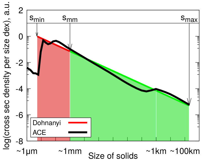
Figure 1: Schematic of an idealized size distribution. Plotted is the cross section per unit size decade as a function of object’s radius. In these axes, a horizontal line corresponds to a power-law size distribution with $q=3$. Straight red-green line: the Dohnanyi (1969) distribution with $q=3.5$. Black line: a typical outcome of a collisional simulation with the ACE code (run A in Appendix A after 100 Myr of evolution) that assumes a size-dependent critical fragmentation energy $Q_{\mathrm{D}}^{*}$ (see Eq. (1) in Krivov et al. 2018). Red-filled area shows what we refer to as “dust sizes.” It corresponds approximately to the size range that is probed by debris disc observations from optical to (sub)mm wavelengths.

To estimate the mass of a debris disc, we have to extrapolate the mass of the observed dust to the mass of the unobservable dust-producing planetesimals. This can be done with the help of debris disc models that tell us what the size distribution of material from dust to the largest bodies may look like. We first assume that the differential size distribution of material in the disc is $n(s)\propto s^{-q}$ with $q=3.5$. This is the slope expected in an infinite collisional cascade with a constant strength of bodies (Dohnanyi 1969).

The Dohnanyi size distribution, on which we impose some lower and upper cut-offs discussed below, is illustrated in Fig. 1. For comparison, we also show a typical size distribution from a collisional simulation (run A in Appendix A), in which a finite size interval was considered and the size dependence of the critical fragmentation energy was taken into account. These distributions are not very different. The most tangible deviations are seen at dust sizes where radiation pressure is important (red-filled area in Fig. 1). This causes a sharp cutoff below the blowout size (Burns et al. 1979) and some ripples above it (e.g., Campo Bagatin et al. 1994; Durda & Dermott 1997; Krivov et al. 2006; Thébault & Augereau 2007; Wyatt et al. 2011). In some systems, dust grains can also be affected by transport mechanisms (e.g., Poynting-Robertson and solar wind drag) which, in combination with radiation pressure and collisions, may cause further deviations of the slope from the Dohnanyi one (e.g., Krivov et al. 2006; Thébault & Wu 2008; Krivov 2010; Wyatt et al. 2011; Matthews et al. 2014). At larger sizes, but below hundreds of metres, where the bodies are still kept together by molecular forces rather than gravity (“strength regime”), the simulated size distribution is somewhat steeper than the Dohnanyi $q=3.5$ (e.g., Durda & Dermott 1997; O’Brien & Greenberg 2003). Still larger bodies whose strength is set by gravity (“gravity regime”) exhibit a distribution that is flatter than the Dohnanyi one. Finally, the largest bodies, above about $1\,\hbox{km}$ in radius, have collisional lifetimes longer than the simulation time. As a result, they preserve their initial size distribution which, in the simulation shown, was assumed to have a slope of $3.7$. Despite all these deviations from a single $q=3.5$ slope, Fig. 1 shows that overall the Dohnanyi size distribution is a good approximation to more detailed models.

Table 1: Sample of debris discs and their dust and disc mass estimates.

HD	Name	$d$	SpT	$L_{*}$	$M_{*}$	Age	$R$	$\Delta R$	$R_{\mathrm{BB}}$	$f_{\mathrm{d}}$	$M_{\mathrm{d}}$	$M_{\mathrm{disc}}$	$M_{\mathrm{disc}}^{*}$	$s_{\mathrm{km}}$	$M_{\mathrm{disc}}^{\mathrm{min}}$
		(pc)		($L_{\odot}$)	($M_{\odot}$)	(Myr)	(au)	(au)	(au)		($M_{\oplus}$)	($M_{\oplus}$)	($M_{\oplus}$)	(km)	($M_{\oplus}$)
$\cdots$	Kuiper belt	10.0	G2V	1.0	1.0	4567	45.0	10.0	20.0	1.0e-07	6.7e-07	1.0e-02	$\cdots$	$\cdots$	$\cdots$
9672	49 Cet	59.4	A1V	15.8	1.9	40	228.0	310.0	85.4	7.2e-04	2.8e-01	4.2e+03	3.6e+04	0.1	14.3
15115	$\cdots$	45.2	F4IV	3.6	1.3	23	78.2	69.6	55.1	4.6e-04	8.5e-02	1.3e+03	2.7e+03	0.5	7.0
21997	$\cdots$	71.9	A3IV/V	9.9	1.7	30	106.0	88.0	65.4	5.6e-04	9.8e-02	1.5e+03	4.2e+03	0.3	7.2
22049	$\varepsilon$ Eri	3.2	K2Vk:	0.3	0.8	600	69.4	11.4	19.5	4.0e-05	2.4e-03	3.6e+01	9.7e+01	0.3	0.2
39060	$\beta$ Pic	19.4	A6V	8.1	1.6	23	100.0	100.0	24.3	2.1e-03	7.9e-02	1.2e+03	4.1e+03	0.3	5.5
61005	$\cdots$	35.3	G8Vk	0.7	0.9	40	66.4	23.6	21.0	2.3e-03	1.3e-01	2.0e+03	2.0e+03	1.0	14.2
95086	$\cdots$	90.4	A8III	6.1	1.7	15	204.0	176.0	46.5	1.4e-03	3.7e-01	5.6e+03	5.9e+04	0.1	17.7
109085	$\eta$ Crv	18.3	F2V	5.0	1.4	1400	152.0	46.0	52.9	2.9e-05	3.1e-02	4.7e+02	8.1e+02	0.6	2.7
111520	$\cdots$	108.6	F5/6V	3.0	1.3	15	96.0	90.0	58.5	1.1e-03	2.9e-01	4.4e+03	9.6e+03	0.4	23.6
121617	$\cdots$	128.2	A1V	17.3	1.9	16	82.5	54.8	30.0	4.9e-03	2.8e-01	4.3e+03	4.6e+03	0.9	29.3
131488	$\cdots$	147.7	A1V	13.1	1.8	16	84.0	44.0	35.6	2.2e-03	7.2e-01	1.1e+04	7.3e+03	1.6	85.8
131835	$\cdots$	122.7	A2IV	11.4	2.0	16	91.0	140.0	57.0	2.2e-03	3.8e-01	5.8e+03	6.4e+03	0.9	39.1
138813	$\cdots$	150.8	A0V	16.7	2.2	10	105.0	70.0	69.6	6.0e-04	4.3e-01	6.6e+03	1.2e+04	0.5	37.2
145560	$\cdots$	133.7	F5V	3.2	1.4	16	88.0	70.0	22.0	2.1e-03	3.3e-01	4.9e+03	7.3e+03	0.7	30.0
146181	$\cdots$	146.2	F6V	2.6	1.3	16	93.0	50.0	17.0	2.2e-03	1.7e-01	2.6e+03	6.9e+03	0.3	13.3
146897	$\cdots$	128.4	F2/3V	3.1	1.5	10	81.0	50.0	15.6	8.2e-03	2.0e-01	3.0e+03	6.0e+03	0.5	16.7
181327	$\cdots$	51.8	F6V	2.9	1.3	23	86.0	23.2	50.1	2.1e-03	3.2e-01	4.8e+03	5.8e+03	0.8	31.3
197481	AU Mic	9.9	M1Ve	0.1	0.6	23	24.6	31.6	11.9	3.3e-04	1.4e-02	2.2e+02	1.2e+02	1.9	1.8
216956	Fomalhaut	7.7	A4V	16.1	1.9	440	143.1	13.6	72.2	7.5e-05	2.4e-02	3.6e+02	9.6e+02	0.3	1.8
218396	HR 8799	39.4	F0V	5.5	1.5	30	287.0	284.0	123.6	2.5e-04	1.7e-01	2.6e+03	7.5e+04	0.02	5.9

Notes: See Table 1 in Matrà et al. (2018) for references to the stellar and disc parameters. $M_{\mathrm{d}}$ is the dust mass estimated from sub-mm fluxes (Eq. 5). $M_{\mathrm{disc}}$ is the total disc mass, obtained by extrapolation of the dust mass assuming two different power laws between $s_{\mathrm{mm}}=1\,\hbox{mm}$ and $s_{\mathrm{km}}=1\,\hbox{km}$ and between $s_{\mathrm{km}}=1\,\hbox{km}$ and $s_{\mathrm{max}}=200\,\hbox{km}$ (Eq. 9). $M_{\mathrm{disc}}^{*}$ is the total disc mass corrected for the time-dependent transition size $s_{\mathrm{km}}$ (Eq. 20). $M_{\mathrm{disc}}^{\mathrm{min}}$ is the total disc mass up to that size $s_{\mathrm{km}}$ (Eq. 24).

The size distribution in a debris disc has several characteristic sizes. The lower cutoff of the size distribution, $s_{\mathrm{min}}$, is close to the radiation pressure blowout limit (e.g., Pawellek & Krivov 2015). This is generally on the order of $1\,\mu\hbox{m}$, with the exact value depending on the luminosity and mass of the central star and the dust composition (e.g., Kirchschlager & Wolf 2013). Another characteristic size, $s_{\mathrm{mm}}$, is the maximum size of particles that we refer to as “dust.” A commonplace choice, which we also make here, is to set $s_{\mathrm{mm}}=1\,\hbox{mm}$, so that it corresponds to the radius of the particles that are most efficiently probed by (sub)mm observations of disc thermal emission. Also, this is the size of the grains above which non-gravitational effects such a radiation pressure can be assumed to be negligible. As explained above, the details of the size distribution between $s_{\mathrm{min}}$ and $s_{\mathrm{mm}}$ are still not fully understood. Therefore, in this paper we circumvent potential uncertainties by working with dust masses derived from (sub)mm thermal emission fluxes (with a caveat that the size distribution at dust sizes indirectly affects conversion of fluxes to dust masses, see Sect. 3.1).

Finally, there is an upper cutoff to the size distribution at $s_{\mathrm{max}}$. In this work we consider a nominal value of $200\,\hbox{km}$, but this is varied in later sections. The justification for this choice is two-fold. First, this value is close to the radius of the largest objects in the cold classical Kuiper belt, although the size distribution in the Kuiper belt steepens to values $\gg 4$ already above $\sim 50$–$100\,\hbox{km}$ (e.g., Bernstein et al. 2004). Second, this is about the size of the largest planetesimals that are built in state-of-the-art planetesimal formation models prior to the onset of runaway growth or pebble accretion. This equally applies to models based on incremental collisional growth ($50$–$100\,\hbox{km}$; see, e.g., Kobayashi et al. 2016) and those invoking pebble concentration ($80$–$600\,\hbox{km}$; see, e.g., Schäfer et al. 2017).

As the size distribution slope is less than $4$, the mass of the disc $M_{\mathrm{disc}}$ is dominated by the largest bodies of size $s_{\mathrm{max}}$: $M_{\mathrm{disc}}\propto s_{\mathrm{max}}^{4-q}$. This means that the total disc mass in bodies, say, up to $200\,\hbox{km}$ is radius, must be higher than the dust mass in mm-sized particles, $M_{\mathrm{d}}$ (which are probed by sub-mm observations), by 4 orders of magnitude (for $q=3.5$). Taking $M_{\mathrm{d}}\sim 10^{-1}M_{\oplus}$, as appropriate for bright debris discs (see, e.g., Fig. 34 in Holland et al. 2017), gives $M_{\mathrm{disc}}\sim 1000M_{\oplus}$, which is close to the the maximum possible mass of a debris disc, as discussed above.

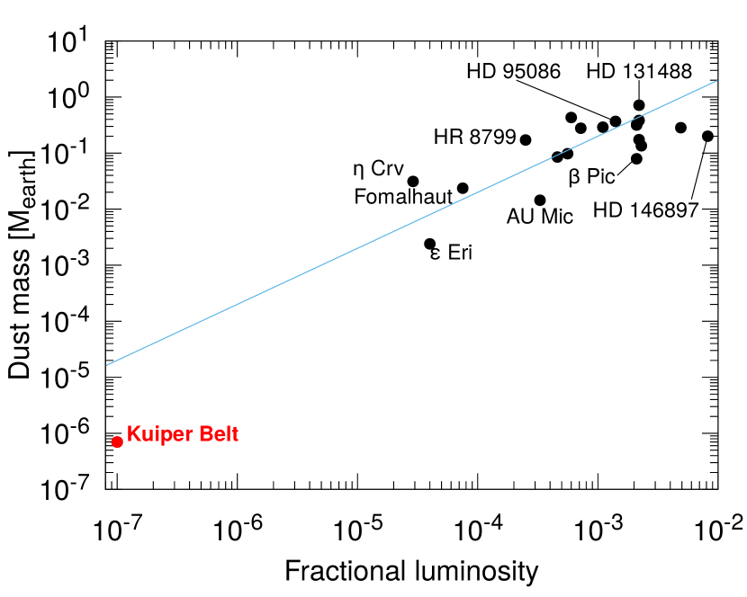
Figure 2: Dust masses of debris discs in our sample. Thin line is the expected $M_{\mathrm{d}}\propto f_{\mathrm{d}}$ dependence. Some of the prominent discs are labeled. Red circle shows the Solar system’s Kuiper belt for comparison.

To get more accurate estimates of the debris disc mass, we now select a set of well-known debris discs. To this end, we take a sample of discs for which resolved images have been taken with ALMA or SMA from Matrà et al. (2018). Their Table 1 lists the luminosity $L_{\star}$, mass $M_{\star}$, and an age estimate of the central star, as well as the characteristic radius $R$ and radial extent $\Delta R$ of each disc. A number of other quantities useful for the analysis, such as the fractional luminosity $f_{\mathrm{d}}$ of each disc, are also given. Finally, total (sub)mm fluxes for each of the discs, $F_{\nu}$, are available. From these, it is easy to calculate the dust mass (i.e., the mass of grains with radii from $s_{\mathrm{min}}$ to $s_{\mathrm{mm}}=1\,\hbox{mm}$):

$$M_{\mathrm{d}}\approx{F_{\nu}d^{2}\over\kappa B_{\nu}(T_{\mathrm{d}})},$$ (5)

where $d$ is the distance to the disc host star, $\kappa$ is the dust opacity (which we assume to be $1.7\,\hbox{cm}^{2}\,\hbox{g}^{-1}(850\,\mu\hbox{m}/\lambda)$ for consistency with previous studies, e.g., Zuckerman & Becklin 1993; Holland et al. 1998; Holland et al. 2017), and $B_{\nu}$ is the black body emission intensity for the dust temperature $T_{\mathrm{d}}$. The latter can be inferred from a disc’s “black body” radius $R_{\mathrm{BB}}$, i.e., the radius that a disc of a given temperature (consistent with the observed spectral energy distribution, SED) would have if its grains were absorbing and emitting as black bodies: $T_{\mathrm{d}}=278\,\hbox{K}(L_{*}/L_{\odot})^{1/4}(R_{\mathrm{BB}}/\,\hbox{au})^{-1/2}$. The total disc mass in bodies up to the radius $s_{\mathrm{max}}$ is calculated as

$$M_{\mathrm{disc}}=M_{\mathrm{d}}\left(s_{\mathrm{max}}\over s_{\mathrm{mm}}\right)^{4-q}.$$ (6)

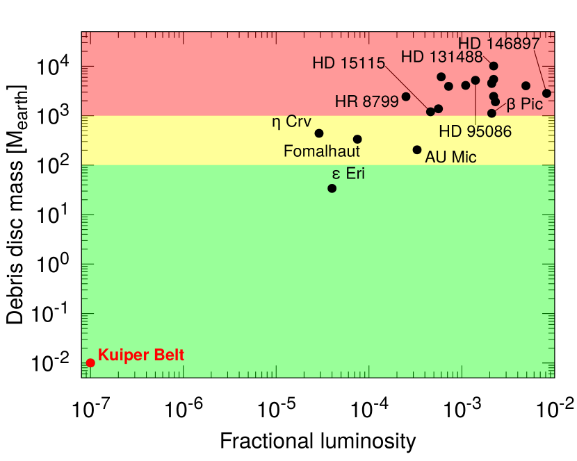
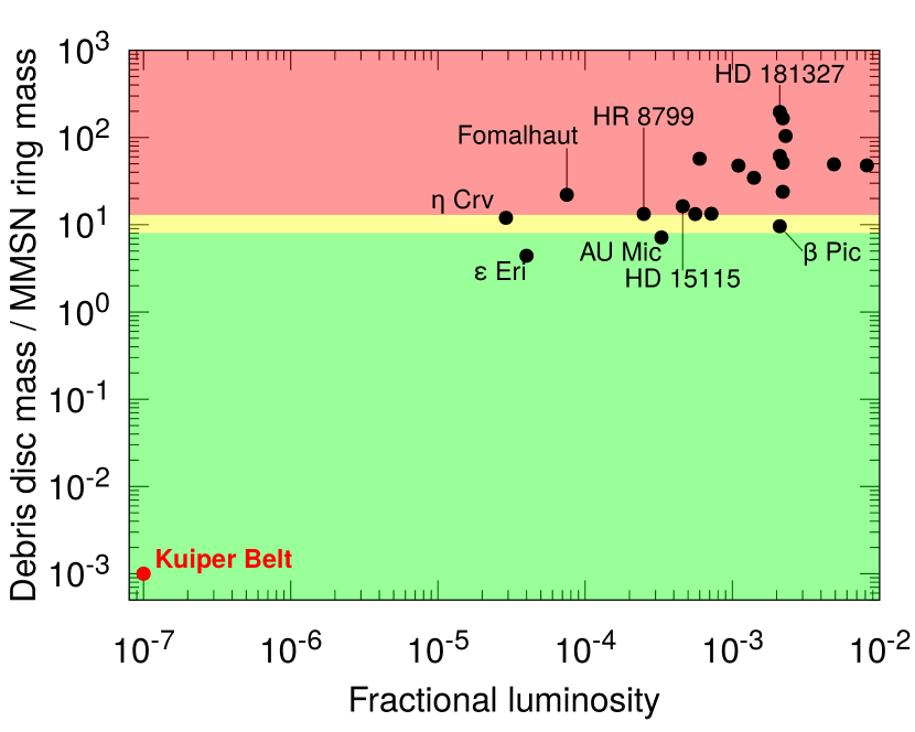
Figure 3: Total mass for the same selection of debris discs, estimated under the assumption of the Dohnanyi collisional cascade ($q=3.5$) in the size range from $1\,\hbox{mm}$ to $200\,\hbox{km}$. Top: disc masses in the units of Earth masses. Bottom: disc masses in the “MMSN units.” Traffic light-style background colors mark the allowed (green) and forbidden (red) areas, and a boundary between them, corresponding the the “maximum debris disc mass” (yellow).

Of the 26 sources in Matrà et al. (2018), we selected 20 with best-quality data (L. Matrà, pers. comm.). All of these were observed with ALMA in bands 6 ($\lambda\approx 1.3\,\hbox{mm}$) or 7 ($\lambda\approx 850\,\mu\hbox{m}$). As a reference, to this sample we added the Kuiper belt of our Solar system with $R=45\,\hbox{au}$, $\Delta R=10\,\hbox{au}$, $f_{\mathrm{d}}=10^{-7}$ (Vitense et al. 2012). To obtain an estimate of the dust mass in the Kuiper belt in the same way as for extrasolar discs, we need a dust flux at some sub-mm wavelength that would be detected from the Kuiper belt if it were observed from afar. That wavelength and the distance at which the Kuiper belt is placed can be taken arbitrarily, and we use $F_{\nu}=1.48\mu\mathrm{Jy}$ at $850\,\mu\hbox{m}$, as predicted for the Kuiper belt if seen from a 10 pc distance (see Fig. 8 in Vitense et al. 2012). Note that, since the thermal emission of the Kuiper belt has not been detected, the fractional luminosity and the emission flux are model-dependent and are uncertain by a factor of a few (see, e.g., Poppe et al. 2019, and references therein). However, this uncertainty is unimportant for our purposes, as we only wish to demonstrate that the Kuiper belt is not affected by the mass problem.

The discs of the resulting sample and their essential parameters are listed in Table 1. The resulting dust masses from Eq. (5) are also given in Table 1 and shown in Fig. 2 against dust fractional luminosity. As expected there is an approximately linear correlation between these two quantitites.

Applying now Eq. (6) with $q=3.5$ yields the top panel in Fig. 3. The mass predicted for the Kuiper belt from its dust mass is low ($\sim 0.01M_{\oplus}$), but pretty much consistent with the values inferred in detailed analyses of TNO surveys (e.g., Fraser et al. 2014). The masses of all extrasolar discs in the sample are by 3–6 orders of magnitude higher and increase with the fractional luminosity as they should from Eq. (5). While for some of the discs ($\varepsilon$ Eri, AU Mic, Fomalhaut, $\eta$ Crv) the total mass lies between $50$–$1000M_{\oplus}$, the other discs appear to be unfeasibly massive. The largest values we obtain are as large as $M_{\mathrm{disc}}\sim 10^{4}M_{\oplus}$!

We can also view these results in a different way, measuring the disc masses in the units of the Minimum Mass Solar Nebula (MMSN; Weidenschilling 1977a; Hayashi 1981). Following Kenyon & Bromley (2008), we adopt the surface density of solids in the MMSN in the form

$$\Sigma(r)=\Sigma_{0}\;r^{-3/2},$$ (7)

where $\Sigma_{0}=29.6\,\hbox{g}\,\hbox{cm}^{-2}(M_{\star}/M_{\odot})$ and the distance from the star $r$ is measured in  au. Note that this MMSN definition includes $M_{\star}$ to account for the fact that the protoplanetary disc masses are roughly proportional to the stellar masses (e.g., Williams & Cieza 2011). We then compute the mass that a debris disc with a radius $R$ and width $\Delta R$ (measured in  au) would have if it had the MMSN surface density profile,

$$M_{\mathrm{MMSN}}=4\pi\Sigma_{0}\left[\left(R+\Delta R/2\right)^{1/2}-\left(R-\Delta R/2\right)^{1/2}\right],$$ (8)

and define $x_{\mathrm{m}}\equiv M_{\mathrm{disc}}/M_{\mathrm{MMSN}}$ to be the disc mass “in MMSN units.”

The result is shown in the bottom panel in Fig. 3. Most of the discs in our sample would have $x_{\mathrm{m}}$ greater than 10 (up to $\sim 200$). However, only surface densities of PPDs below $\sim 10$ times MMSN are commonly considered plausible. One reason for this is that higher densities would violate the Toomre (1964) gravitational stability criterion (e.g., Kuchner 2004; Rafikov 2005), while the vast majority of PPDs observed in young stellar associations were found to be gravitationally stable at all radii (e.g., Isella et al. 2009).

One caveat of measuring the disc masses in the MMSN units is that the $-3/2$ radial slope in the MMSN definition of equation (7) does not necessarily represent actual conditions in extrasolar systems. Indeed, slopes of PPDs inferred from (sub)mm obsrvations are generally flatter (e.g., Andrews et al. 2009, 2010), whereas “Minimum-Mass Extrasolar Nebulae” constructed from known extrasolar planet populations have steeper surface densities (Kuchner 2004; Chiang & Laughlin 2013).

2.4 Disc mass estimates including planetesimal formation model predictions

The idealized models described above just consider a size distribution that is set by a collisional cascade. To arrive at a more realistic model, we must take into account that the largest planetesimals, especially in younger systems, are not part of the cascade, because their collisional lifetime may be longer than the system’s age. Such planetesimals preserve their original size distribution they acquired at the formation stage. Although contributing only little to the production of the observed dust, these are nevertheless important for understanding the mass budget, since they contain most of the debris disc mass.

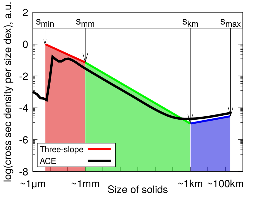
Figure 4: A more realistic size distribution. Three-segment (red-green-blue) line: a combination of three power laws with different slopes that are expected at the dust sizes (red-filled area), sizes of planetesimals that are collisionally ground by the cascade (green), at sizes of largest planetesimals that retain their primordial size distribution (blue). Black line: a typical outcome of a collisional simulation with the ACE code (run B in Appendix A after 100 Myr of evolution) that takes a primordial size distribution of planetesimals predicted by pebble concentration models of their formation.

To understand what the primordial size distribution of large planetesimals might look like, we have to take into account the planetesimal formation history. Although several competing models exist, in this paper we consider the possibility that planetesimals form by the “particle concentration”, or “pebble concentration” mechanism (e.g., Haghighipour & Boss 2003; Johansen et al. 2007; Cuzzi et al. 2008, 2010; Chambers 2010; Johansen et al. 2015; Simon et al. 2016, 2017). In this mechanism, pebble-sized (typically mm–cm sized) particles in a PPD concentrate in certain zones of the disc, for instance by streaming instability (SI), followed by a local gravitational collapse to form planetesimals in just 3–5 Myr (e.g., Johansen et al. 2015; Carrera et al. 2017).

These models make predictions for the sizes of newly formed planetesimals. The size distribution above $s\sim 1\,\hbox{km}$ should be much flatter than the Dohnanyi one, $q_{\mathrm{big}}=2.8\pm 0.1$ for a broad range of possible model parameters (Johansen et al. 2015; Simon et al. 2016, 2017; Abod et al. 2019). This slope should extend to radii of a few hundred kilometres (with $s_{\mathrm{max}}=200\,\hbox{km}$ being a typical value) before it steepens towards Pluto-sized dwarf planets (Schäfer et al. 2017).

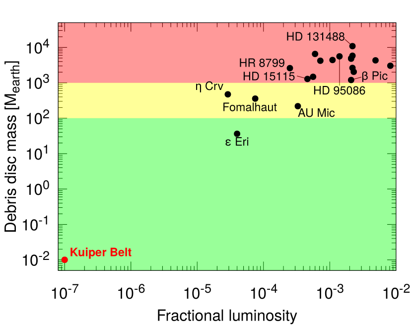
Figure 5: Same as Fig. 3 top, but assuming that planetesimals form by the streaming instability (SI). This incorporates the “initial mass function” of bodies predicted by the SI-based models of their formation with $q_{\mathrm{big}}=2.8$ up to a size of $200\,\hbox{km}$.

The size distribution expected from the collisional disruption of planetesimals with such an initial size distribution can be approximated by a combination of three power laws (Fig. 4). One would be valid at dust sizes, from the blowout limit to some size $s_{\mathrm{mm}}\sim 1\,\hbox{mm}$, where radiation pressure is important. As a nominal value, we take $q=3.5$ (see a discussion in Sect. 3.2.3). This slope $q$ can further be altered by transport mechanisms, such as Poynting-Robertson and stellar wind drag. Although these are usually of importance for low-mass discs that are not considered here, they may also affect discs of late-type stars with strong winds. Two discs in our sample, $\varepsilon$ Eri (Reidemeister et al. 2011) and AU Mic (Schüppler et al. 2015), belong to this category. As explained in Sect. 2.3, this slope does not affect the results of our analysis considerably (except that it contributes to opacity, see Sect. 3.1, and slightly affects the extrapolation of the dust mass to the disc mass, entering Eq. 9 below). However, it is included to acknowledge the uncertainty that is inevitable when considering the quantity of small dust that may be present, e.g., as probed in infrared and scattered light observations.

The second slope $q_{\mathrm{med}}$, extending from $s_{\mathrm{mm}}\sim 1\,\hbox{mm}$ to $s_{\mathrm{km}}\sim 1\,\hbox{km}$, is set by the collisional cascade and is somewhat steeper than the Dohnanyi one. We fix it to $q_{\mathrm{med}}=3.7$. Finally, the third slope $q_{\mathrm{big}}$ is expected for the bodies larger than $s_{\mathrm{km}}$, which are not part of the cascade. As discussed above, it should be the primordial one predicted by planetesimal formation models, i.e., $q_{\mathrm{big}}\approx 2.8$. Figure 4 shows that the analytical three-phase size distribution with slopes $q$, $q_{\mathrm{med}}$ and $q_{\mathrm{big}}$ agrees well with the collisional simulation.

We now apply this three-slope size distribution to the same sample of debris discs. Equation (6) is replaced by

$$M_{\mathrm{disc}}=M_{\mathrm{d}}\;{4-q\phantom{{}_{b}ig}\over 4-q_{\mathrm{big}}}\left(s_{\mathrm{km}}\over s_{\mathrm{mm}}\right)^{4-q_{\mathrm{med}}}\left(s_{\mathrm{max}}\over s_{\mathrm{km}}\right)^{4-q_{\mathrm{big}}}.$$ (9)

Disc masses obtained with Eqs. (5) and (9) are given in the $M_{\mathrm{disc}}$ column of Table 1 and plotted in Fig. 5. The problem gets even worse, because there is now a lot of “dead” mass in bodies larger than $\sim 1\,\hbox{km}$. These big objects are not needed to reproduce the debris disc data with collisional models, although they are expected to be present from the planetesimal formation simulations. However, a steeper slope $q_{\mathrm{med}}$ in Eq. (5) compared to $q$ in Eq. (6) reduces the total mass. As a result, the disc masses shown in Fig. 5 are only 7% larger than those depicted in Fig. 3.

Equation (9) shows that the disc mass estimate $M_{\mathrm{disc}}$ is proportional to $s_{\mathrm{km}}^{q_{\mathrm{big}}-q_{\mathrm{med}}}\propto s_{\mathrm{km}}^{-0.9}$. Thus any uncertainty in $s_{\mathrm{km}}$ would translate to a similar uncertainty in $M_{\mathrm{disc}}$. To create Fig. 5, we simply fixed $s_{\mathrm{km}}$ to $1\,\hbox{km}$. However, this size that separates the primodial planetesimal population from the collisionally processed ones increases with time, as larger and larger bodies get involved in the cascade. The size dependence of $s_{\mathrm{km}}$ on age is discussed in more detail in Sect. 3.3, where also quantitative estimates are given. We will particularly show that using a time-variable $s_{\mathrm{km}}$ in Eq. (9) would not significantly affect the mass estimate for any discs, regardless of their age.

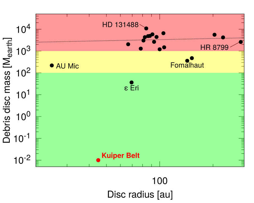
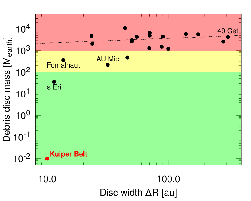
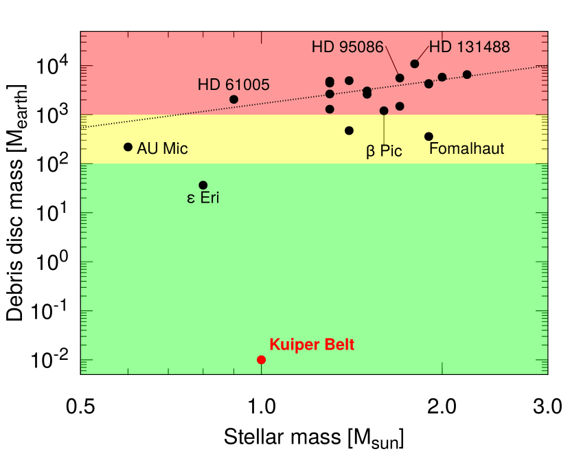
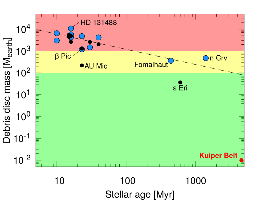
Figure 6: Dependence of the inferred total disc mass on (a) the disc radius, (b) the disc width, (c) the stellar mass, and (d) the stellar age. Dashed lines in each plot are best power-law fits through the data (without the Kuiper belt). In panel (d), larger blue symbols mark discs in which gas detections have been reported, whereas black symbols stand for discs without such detections. Otherwise, symbols, labels, and filled areas are as in Figs. 3 and 5.

In principle, pebble concentration models of planetesimal formation have more implications than just introducing a primordial population of planetesimals with a flat size distribution. The same models predict the planetesimals to be loosely bound, fragile “pebble piles”. This prediction is backed up by a bulk of evidence that comets in the Solar system are porous “pebble piles” (e.g., Blum et al. 2017), which probably traces back to their formation mechanisms. Similarly, (non-differentiated) asteroids (e.g., Britt et al. 2002) are known to have a significant macro-porosity and are thought to have been turned into rubble piles by repeated shattering collisions with subsequent gravitational reaccumulation. As a result, small bodies in the Solar system have relatively low densities. For instance, a density of $0.533\,\hbox{g}\,\hbox{cm}^{-3}$ was measured for the comet 67/P (Pätzold et al. 2016). Similar values were determined for Arrokoth (Stern et al. 2019), and densities in the $0.5\ldots 1\,\hbox{g}\,\hbox{cm}^{-3}$ range were inferred for a suite of Kuiper-belt objects up to hundreds of km in size (e.g., Brown 2012, and references therein).

By analogy with the Solar system, we may expect large planetesimals in extrasolar systems to have low densities as well. To account for this, we can allow solids in the three size ranges of the broken power-law size distribution to have different bulk densities ($\rho$, $\rho_{\mathrm{med}}$, and $\rho_{\mathrm{big}}$). In this case, Eq. (9) needs to be generalized. This generalisation depends on how exactly the three-slope distribution is defined. If we require that the differential size distribution is continuous at transition points $s_{\mathrm{mm}}$ and $s_{\mathrm{km}}$ where the density changes, then the right-hand side of Eq. (9) will acquire an additional factor $\rho_{\mathrm{big}}/\rho$ (the density $\rho_{\mathrm{med}}$ does not enter the equation). Taking $\rho_{\mathrm{big}}\sim 0.5\ldots 1\,\hbox{g}\,\hbox{cm}^{-3}$ for large planetesimals and $\rho=2.35\,\hbox{g}\,\hbox{cm}^{-3}$ for dust (see Appendix A) would reduce the total disc mass estimates by a factor of two to five. If, instead, we require the differential mass distribution to be continuous, Eq. (9) will remain valid as written. We expect that the latter model, i.e., requiring that the mass distribution stays continuous at the density jumps, is a better approximation to reality, simply because it is the mass and not the number of particles that is conserved in destructive collisions. Thus the values of $M_{\mathrm{disc}}$ listed in Table 1 and depicted in Fig. 5 should hold for the size-dependent density.

Further, if planetesimals in extrasolar systems are pebble piles or rubble piles, they will be quite easy to destroy even in low-energy collisions. This primarily applies to bodies with sizes between $\sim\,\hbox{cm}$ and $\sim\,\hbox{km}$, i.e., between the strength and gravity regimes. This means that more realistic simulations would have to consistently use a “pebble-pile”-like critical fragmentation energy prescription (see Eqs. 2–4 in Krivov et al. 2018, and their Fig. 1). Applying it would result in a deep minimum in the size distribution at sizes between $\sim\,\hbox{cm}$ and $\sim\,\hbox{km}$ (see Fig. 4 in Krivov et al. 2018). However, it is possible to show that the presence of this minimum is unimportant for the discussion of the mass budget, as long as the disc is in a collisional steady state. This is because the amount of the observed dust is given by a product of the grain lifetime and the dust production rate, where the latter is equal to the mass loss rate of the largest bodies that are in the collisional equilibrium (because in a steady-state system all the mass lost by bigger objects is transferred to smaller objects at the same rate). The mass loss rate of the biggest planetesimals, in turn, is proportional to the amount of those bodies in the system. As a consequence, the amount of dust in a steady-state disc for a given amount of the largest planetesimals that are in the collisional equiulibrium is independent of the fragmentation efficiency of intermediate-sized bodies. Nevertheless, our $Q_{\mathrm{D}}^{*}$ prescription outside the fragile mid-size range also has uncertainties of a factor of few. This may affect the values of $s_{\mathrm{km}}$ derived in our simulations and so the estimates of the total disc mass (see Sect. 3.3).

2.5 Dependence of disc mass on the host star and disc extent

We now look at the total disc mass against parameters other than the dust fractional luminosity. Since our sample contains only 20 discs, we cannot make any statistically significant conclusions. Nevertheless, this analysis may show which parameters make some discs more affected by the mass problem than the others, thus giving some hints about the origin of the problem. Besides, we check whether any known trends are also visible in our sample.

Two upper panels in Fig. 6 check how the estimated mass is related to the disc geometry. Since the disc mass is proportional to $R^{2}(\Delta R/R)\Sigma(R)$, where the surface density of solids $\Sigma(R)\propto R^{-p}$ is commonly assumed to gently decrease with the distance from the star ($1\la p\la 2$), we may expect that larger discs tend to be more massive. This is neither supported nor ruled out by Fig. 6a; the best fit is $M_{\mathrm{disc}}\propto R^{0.17\pm 0.37}$. Similarly, we may expect radially extended discs to have higher masses on the average compared to the narrow ones. Figure 6b confirms this, albeit at a low significance level. The best fit is $M_{\mathrm{disc}}\propto\Delta R^{0.22\pm 0.20}$. Note, however, that two of the three lowest-mass discs (Fomalhaut and $\varepsilon$ Eri) are the narrowest.

The remaining two panels in Fig. 6 depict the disc masses against stellar parameters. There might be a weak trend towards higher debris disc masses around more massive stars (Fig. 6c). We find $M_{\mathrm{disc}}\propto M_{*}^{1.63\pm 0.79}$. Besides, the masses of discs around the two lowest-mass stars in the sample, AU Mic and $\varepsilon$ Eri, are lower that those of the other discs. This could possibly be attributed to that fact that debris disc progenitors, protoplanetary discs, tend to have lower masses around lower-mass primaries (see Sect. 2.2). However, there are various observational biases here that need to be considered given that this is not a statistical sample. Finally, Fig. 6d demonstrates that three discs around older stars ($0.4$–$1.4\,\hbox{Gyr}$) in our sample reveal about an order of magnitude lower masses than those in young systems ($10$–$40\,\hbox{Myr}$). The formal fit through the data yields $M_{\mathrm{disc}}\propto T_{\mathrm{age}}^{-0.70\pm 0.34}$. This likely reflects a well-known long-term decay of debris discs (see Sect. 2.1).

3 Possible solutions

Krivov et al. (2018) listed and briefly discussed several possible solutions to the debris disc mass problem. Here we revisit some of them and consider a few other possibilities.

3.1 Uncertainty in the dust mass?

Since the total mass of a debris disc is directly proportional to the dust mass inferred from observations (Eq. 9), the question is, how reliable that dust mass is. The largest uncertainty in calculating it arises from the mass absorption coefficient $\kappa$ in Eq. (5). In the above analysis we set it to $1.7\,\hbox{cm}^{2}\,\hbox{g}^{-1}(850\,\mu\hbox{m}/\lambda)$, which is a common choice in the (sub)mm literature. However, the actual opacity depends on a number of factors. Indeed, the opacity at a given wavelength is equal to the ratio of the absorption cross section of the disc material and the dust mass:

$$\kappa(\lambda)={\int\limits_{s_{\mathrm{min}}}^{s_{\mathrm{max}}}\pi s^{2}n(s)Q_{\mathrm{abs}}(s,\lambda)ds\over\int\limits_{s_{\mathrm{min}}}^{s_{\mathrm{mm}}}\frac{4}{3}\pi\rho_{\mathrm{d}}s^{3}n(s)ds}.$$ (10)

Note that the sub-mm flux in a $q\approx 3.5$ size distribution is dominated by particles in the size range from $\sim 100\,\mu\hbox{m}$ to $\sim 10\,\hbox{cm}$ (see, e.g., Fig. 5 in Wyatt & Dent 2002). For some materials, even grains larger than $\sim 10\,\hbox{cm}$ can make non-negligible contribution to sub-mm fluxes (Löhne 2020). This is why the integral in the numerator extends over the full range of sizes from $s_{\mathrm{min}}$ to $s_{\mathrm{max}}$, thus including not only dust, but also larger material, since it may contribute to the absorption cross section and thus also to the observed thermal emission fluxes $F_{\nu}$ in Eq. (5). In contrast, the integral in the denominator is taken from $s_{\mathrm{min}}$ to $s_{\mathrm{mm}}=1\,\hbox{mm}$ to represent the mass of dust. Defined this way, the opacity $\kappa$ gives the emitting cross-sectional area per mass in $<1\,\hbox{mm}$ grains assuming the size distribution to extend to larger sizes.

Dust opacity in astrophysical environments has been in the focus of interest for decades, motivated by studies of interstellar medium in general, star-forming clouds and protoplanetary discs (e.g., Draine & Lee 1984; Beckwith & Sargent 1991; Pollack et al. 1994; Henning et al. 1995; Semenov et al. 2003; Draine 2006, and references therein). In all these applications, most of the mass is thought to be in dust rather than big objects. Consequently, the vast majority of previous studies on opacity considered single grain sizes or a size distribution that is truncated at a size on the order of mm or cm. In the latter case, it is a common practise to use both integrals in Eq. (10) with the same upper limit that is set to somewhere in the mm to cm range. While this is sufficient for distributions in which there is little mass in objects larger than cm, this is not the case in a debris disc. This is why in the following discussion it is essential to use Eq. (10) as written, with the caveat that caution is required when comparing opacities discussed here with those reported in the literature.

Equation (10) shows that the opacity depends on the material composition and morphology of dust grains (which determine the absorption efficiency $Q_{\mathrm{abs}}$ and the bulk density of dust $\rho_{\mathrm{d}}$). The minimum size $s_{\mathrm{min}}$ is closely related to the radiation pressure blowout limit (e.g., Pawellek & Krivov 2015) and so, also depends on the dust composition. However, the dependence on $s_{\mathrm{min}}$ is weak, since particles of size $s_{\mathrm{min}}$ emit inefficiently and contain little mass. Finally, the opacity depends on the size distribution $n(s)$ – not only at dust sizes but, for some materials, also at larger sizes if these contribute to the thermal emission at wavelength $\lambda$.

To see to what extent all these parameters may alter the opacity, we chose $\lambda=1\,\hbox{mm}$ as a reference wavelength, lying between the two ALMA bands ($\approx 850\,\mu\hbox{m}$ and $\approx 1.3\,\hbox{mm}$) in which discs of our sample were observed. We start with considering “astronomical silicate” (Draine 2006) as the dust composition, which is a traditional (although not really justified) choice in debris disc modeling. Its bulk density was taken to be $\rho_{\mathrm{d}}=3.5\,\hbox{g}\,\hbox{cm}^{-3}$, and the absorption efficiency was calculated from the optical constants by using the Mie algorithm of Wolf & Voshchinnikov (2004). Assuming $q=3.5$ and $s_{\mathrm{min}}=1\,\mu\hbox{m}$, the resulting opacity $\kappa=5.14\,\hbox{cm}^{2}\,\hbox{g}^{-1}$. However, it varies with the size distribution slope and the minimum grain size. For $3\leq q\leq 4$ and $s_{\mathrm{min}}=1\,\mu\hbox{m}$, we determine $2.34\,\hbox{cm}^{2}\,\hbox{g}^{-1}\leq\kappa\leq 14.6\,\hbox{cm}^{2}\,\hbox{g}^{-1}$. As noted above, the dependence on $s_{\mathrm{min}}$ is weak, and is only noticeable for steeper size distributions, for which smaller particles make a larger contribition to the cross section. As an example, assuming $q=4$ and varying $s_{\mathrm{min}}$ from $0.5\,\mu\hbox{m}$ to $5\,\mu\hbox{m}$ changes $\kappa$ from $2.15\,\hbox{cm}^{2}\,\hbox{g}^{-1}$ to $2.95\,\hbox{cm}^{2}\,\hbox{g}^{-1}$.

Since we do not know what the composition of debris dust looks like in reality, we can invoke results of laboratory measurements with THz techniques performed for some materials of potential astrophysical relevance. As an example, we consider crystalline water ice (Reinert et al. 2015), forsterite (Mutschke & Mohr 2019), pyroxene (H. Mutschke & P. Mohr, in prep.), and amorphous carbon (Zubko et al. 1996). At $\lambda=1\,\hbox{mm}$ and a temperature of $100\,\hbox{K}$, and assuming a size distribution with $q=3.5$ and $s_{\mathrm{min}}=1\,\mu\hbox{m}$, the opacity varies from $\sim 0.48\,\hbox{cm}^{2}\,\hbox{g}^{-1}$ for forsterite and $\sim 1.34\,\hbox{cm}^{2}\,\hbox{g}^{-1}$ for crystalline water ice through $\sim 3.30\,\hbox{cm}^{2}\,\hbox{g}^{-1}$ for pyroxene to $\sim 14.4\,\hbox{cm}^{2}\,\hbox{g}^{-1}$ for amorphous carbon. Interestingly, the opacity $1.7\,\hbox{cm}^{2}\,\hbox{g}^{-1}(850\,\mu\hbox{m}/\lambda)$ assumed here, or $1.45\,\hbox{cm}^{2}\,\hbox{g}^{-1}$ at $1\,\hbox{mm}$, is in the middle of the range for these extreme assumptions.

By analogy with compositional constraints derived for the Solar system comets (e.g. 67/P, see Fulle et al. 2016), it is likely that the actual debris dust is a mixture of pure materials like these. However, neither the fractions of the components nor the way they are mixed (e.g., layer-like or inclusion-like) are known. Additional uncertainties come from (unknown) porosity of grains (Henning & Stognienko 1996), as well as from the temperature dependence of the opacity. For all of the materials listed above, opacity tends to decrease toward lower temperatures (Reinert et al. 2015; Häßner et al. 2018; Potapov et al. 2018; Mutschke & Mohr 2019, H. Mutschke & P. Mohr, in prep.).

To summarize, the assumed debris dust opacity is uncertain, perhaps by a factor of several. We argue, however, that this uncertainty is not of crucial importance for the mass problem. For example, were the opacity of the debris material lower than commonly assumed, correcting for this would further increase the inferred dust mass and so also the total mass of the discs. However, this could equally affect the inferred masses of protoplanetary discs and thus proportionally increase the “‘maximum mass of a debris disc.” As a result, this would just “upscale” the entire mass problem without increasing or reducing the tension between the estimated and maximum possible masses of debris discs, albeit implying that PPDs are more prone to gravitational instability (Toomre 1964).

3.2 An overall steeper size distribution?

The above discussion of the mass problem relies upon models of the collisional cascade that predict a certain slope of the size distribution across many orders of magnitude of particle sizes, from mm-sized grains to km-sized objects – i.e., the largest objects that can be destroyed by collisions within the age of the system. The question arises, how certain these predictions actually are. Should, for some reasons, the overall size distribution slope be somewhat steeper, the same amount of dust could be sustained by a planetesimal population of lower mass. One possibility to change the slope is to allow the mean relative velocities $v$ in the disc to be size-dependent. Assuming that $Q_{\mathrm{D}}^{*}\propto s^{\gamma}$ and $v\propto s^{p}$, Kobayashi & Tanaka (2010) and Pan & Schlichting (2012) showed that the slope of the differential size distribution is given by

$$q={21+\gamma-2p\over 6+\gamma-2p},$$ (11)

leading for $p>0$ to steeper slopes than those computed under the assumption of size-independent relative velocities.

Several effects are responsible for the evolution of the relative velocities amongst particles in a debris disc (e.g., Stewart & Wetherill 1988). In addition to gas which is discussed in Sect. 3.2.2, the effects of viscous stirring, damping by inelastic collisions, and damping by dynamical friction are most important and discussed in Sect. 3.2.1.

3.2.1 Collisional damping

Pan & Schlichting (2012) found analytically power-law solutions for the combined steady-state size and velocity distributions in collisional debris discs. In one of the regimes they considered (see their Fig. 3), they found $p$ to lie between $0.16$ and $0.5$ in the size range from $1\,\hbox{m}$ to $\gg 1\,\hbox{km}$, and confirmed this analytic prediction by direct numerical simulations with a collisional code. There are no reasons to expect that this moderately positive slope $p$ would be different below the lowest cutoff of their setup, $1\,\hbox{m}$, down to the smallest objects still unaffected by radiation pressure, say $\sim 1\,\hbox{cm}$.

Based on this result, let us now conservatively assume $p=0.2$ in the size interval from $\sim 1\,\hbox{cm}$ to $\sim 1\,\hbox{km}$. Taking $\gamma=-0.34$ as appropriate for the strength regime, Eq. (11) gives $q=3.85$. Plugging this into our toy model including the primordial size distribution from planetesimal formation simulations, and applying to the same sample of debris discs as before, we estimated disc mass would reduce by a factor of 8. The mass problem would essentially be solved, at least for the majority of the discs in our sample.

If this effect is at work, this might be in line with the in-depth collisional simulations that aimed at reproducing the observed resolved thermal emission and/or scattered light images of several individual systems (e.g., Reidemeister et al. 2011; Löhne et al. 2012; Schüppler et al. 2014, 2015, 2016), from which parent planetesimals with eccentricities $\sim 0.01$…$0.05$ were inferred. These values are lower than those typical for the Kuiper belt, and also lower than those that might be expected from the presence of known stirring planets in some systems (such as HR 8799). However, the conclusions that the eccentricities are low were based on ACE simulations that assumed the same excitation across the range of sizes, which is a limitation of the current ACE code. Strictly speaking, these conclusions apply to the eccentricities of cm-sized grains (the destruction of which produces visible dust), and not to those of larger planetesimals. Had collisional damping been included, and had it been efficient, these lower eccentricites of cm-sized grains could have resulted from a more stirred population of km-sized and larger planetesimals. In the above example where $p=0.2$, the latter would be an order of magnitude higher.

However, the work by Pan & Schlichting (2012) rests on a number of assumptions that all were necessary to keep the problem treatable analytically. One of them is that bullet-target size (or mass) ratios in destructive collisions are close to unity. However, for high-mass-ratio collisions, the damping rate is reduced by a factor of $(m_{\mathrm{p}}/m_{\mathrm{t}})^{2}$, where $m_{\mathrm{p}}$ and $m_{\mathrm{t}}$ are masses of colliders ($m_{\mathrm{p}}\ll m_{\mathrm{t}}$), see Eq. (17) in Kobayashi et al. (2016). This is actually what one would expect under typical debris disc conditions. Indeed, a few debris disc simulations done so far with collisional codes that include viscous stirring and collisional damping effects, do not show any noticeable eccentricity damping towards smaller objects in the centimetre-kilometre size range – see, e.g., Fig. 1 right in Kenyon & Bromley (2008) or Fig. 3 in Kobayashi & Löhne (2014).

One more uncertainty is related to the point made in Sect. 2.4 about planetesimals possibly being “pebble piles”, whose critical fragmentation energy $Q_{\mathrm{D}}^{*}$ in the strength regime is very different from the one of the “monolithic” bodies (Krivov et al. 2018). For such $Q_{\mathrm{D}}^{*}$, the analytic model by Pan & Schlichting (2012) is no longer valid. To our knowledge, the role of the stirring-damping balance in such systems has never been tested in numerical simulations either. We expect that this would make damping less relevant, as the planetesimals are weaker and so the ratio $m_{\mathrm{p}}/m_{\mathrm{t}}$ is even smaller than in the “monolithic case.” However, should a regime in which collisional damping is strong be found in the future, this could provide a natural solution to the disc mass problem.

3.2.2 Secondary gas

Velocity damping may also come from the ambient gas, if there is some in the disc. Debris discs are generally known to be gas-poor, yet a handful of young debris discs, mostly around earlier-type stars, reveal gas in detectable amounts (e.g., Kral et al. 2017). This gas, notably CO, is likely secondary and is released from planetesimals in collisions, i.e., in the same process that creates observable debris dust. Figure 6d shows that in many of the discs with high masses gas has indeed been detected.

To check to what extent gas damping can alter the size distribution, we consider the same system as in runs A and B of Appendix A: an A-type star ($2.16M_{\odot}$, $27.7L_{\odot}$) as a primary and a disc with a radius of $100\,\hbox{au}$ and width of $10\,\hbox{au}$. However, we now take an extreme case of the disc containing $\sim 0.06M_{\oplus}$ of CO gas (as appropriate for the most gas-rich debris discs such as HD 21997 or HD 131835, Kral et al. 2017). The gas is assumed to be co-located with the dust.

Assuming subsonic regime, the stopping time (see, e.g., Weidenschilling 1977b) is given by $T_{\mathrm{stop}}=(\rho_{\mathrm{g}}/\rho_{\mathrm{d}})(s/c_{\mathrm{s}})$, where $\rho_{\mathrm{g}}$ is the spatial density of gas, $\rho_{\mathrm{d}}$ the bulk density of dust (assumed to be $2.35\,\hbox{g}\,\hbox{cm}^{-3}$), and $c_{\mathrm{s}}=\sqrt{(kT_{\mathrm{g}})/(\mu m_{\mathrm{H}})}$ the sound speed in the ambient gas. In the last equation, $k$ is the Boltzmann constant, $\mu$ the molecular weight (which we set to 28 as appropriate for CO gas), and $T_{\mathrm{g}}$ the gas temperature which, for the sake of rough estimates, is taken to be the black body temperature at the disc radius: $T_{\mathrm{g}}\approx 278\,\hbox{K}(L_{*}/L_{\odot})^{1/4}(R/\,\hbox{au})^{-1/2}$. For the gas-rich disc around an A-type star considered here, the stopping time is

$$T_{\mathrm{stop}}\approx 330\left(s\over 1\,\mu\hbox{m}\right)\,\hbox{yr}.$$ (12)

The stopping time is also the timescale on which orbital eccentricities and inclinations of particles can be substantially damped by gas. However, efficient damping is only possible if the damping timescale is shorter that the collisional timescale of the disc solids. The latter can be estimated as (e.g., Wyatt 2005)

$$T_{\mathrm{coll}}\approx{P\over 8\pi f_{\mathrm{d}}}{\Delta R\over R},$$ (13)

where $P=\sqrt{GM_{*}/R^{3}}$ is the orbital period. This is the collisional lifetime of the smallest grains that dominate the cross section (or the optical depth) of the disc. We assume these to have size just above the radiation pressure blowout limit which, for the A-star and grain density of assumed here (see Appendix A), is equal to $6.3\,\mu\hbox{m}$. For a size distribution with a slope $q$, the collisional lifetime of larger grains scales as $T_{\mathrm{coll}}(s)\propto s^{4-q}$ (e.g., Wyatt & Dent 2002; O’Brien & Greenberg 2003; Wyatt et al. 2011). For the same disc and the same A-type star as above, and assuming the $f_{\mathrm{d}}=10^{-4}$, we obtain

$$T_{\mathrm{coll}}\approx 1.1\times 10^{4}\left(s\over 1\,\mu\hbox{m}\right)^{4-q}\,\hbox{yr}.$$ (14)

From Eqs. (12) and (14) with $q=3.5$, we find the condition for efficient damping, $T_{\mathrm{stop}}<T_{\mathrm{coll}}$, to be fulfilled for all grains smaller than about $1\,\hbox{mm}$ in size. As a result, we expect steepening of the size distribution at those sizes (a positive $p$ in Eq. 11). Said differently, this should result in an enhanced dust density compared to that of larger solids.

Note that the total amount of gas mass in such discs can be even higher, as most of the gas mass could be in atomic C and O. In some of the discs, this has directly been confirmed observationally. As an example, in the HD 32297 disc a CO mass of $4\times 10^{-4}M_{\oplus}$ (MacGregor et al. 2018) and a neutral C mass of $3.5\times 10^{-3}M_{\oplus}$ (Cataldi et al. 2020) have been inferred. A larger total mass of gas would mean that gas damping can be efficient at sizes larger than inferred from the above calculation, leading to a stronger alteration of the size distribution compared to the gas-free case. However, in extreme cases, such as the discs with $\sim 0.06M_{\oplus}$ of CO gas quoted above, CO might be self-shielded and so the mass in CO could be comparable to or even greater than that of C (see for example Fig. 6 of Marino et al. 2020) and so the above calculation would be unaffected.

Simple estimates of how strong the effects would be are difficult to make for several reasons. For instance, sufficiently small grains can be swiftly damped so strongly that collisions with like-sized grains would no longer be disruptive. On the other hand, these grains would also collide with larger ones that retain higher dynamical excitation. Sufficiently accurate quantitative predictions for these effects would require a dedicated modeling, taking into account a size distribution and a size-dependent distribution of eccentricities and excitations of grains in the ambient gas environment.

3.2.3 Any signs of damping in mm observations?

In the previous subsections, we argued that damping is not likely to be efficient, except perhaps for sub-mm sizes in some discs with appreciable amount of gas. Regardless of theoretical arguments, it is useful to see whether any signs of damping at such sizes can be seen in observations. Debris disc observations at multiple long (mm to cm) wavelengths to get the spectral index of the emission can be used to constrain size distributions of grains in the size range comparable to the wavelength. A standard method is to use the Draine (2006) equation that relates the measured SED slope in the mm regime to the slope of the dust size distribution. Applying this method to five discs observed with ATCA at $9\,\hbox{mm}$, Ricci et al. (2015) inferred $3.36<q<3.50$, with a typical uncertainty of $0.07$–$0.08$. A similar analysis for a larger selection of discs observed with several facilities at wavelengths from $0.85\,\hbox{mm}$ to $9\,\hbox{mm}$ was done by MacGregor et al. (2016) who derived $3.2<q<3.7$, with a weighted mean of $q=3.36\pm 0.02$. Most recently, Löhne (2020) extended the Draine (2006) formula by lifting several assumptions that are not necessarily fulfilled for debris discs. Applied to a sample similar to that of MacGregor et al. (2016), this model yields the mean slope of $q=3.42\pm 0.04$ and $q=3.55\pm 0.05$, assuming dust composition to be astrosilicate and pyroxene, respectively.

The disc samples used in these analyses included some of the discs that are also part of the Matrà et al. (2018) sample used in this paper. Some of these (e.g., HD 95086 and HD 131835) are among those strongly affected by the mass problem, yet their inferred size distribution slopes are rather low ($q<3.5$). This might argue against steeper distribution, and so also against efficient damping in such discs, at least at sizes smaller than $\sim\,\hbox{cm}$. Of course, for damping to work, the size distribution only needs to be steep at cm–km sizes. However, the damping (be that by gas or collisions) is expected to be more efficient at smaller not larger sizes (e.g., the size of bullets goes down as $Q_{\mathrm{D}}^{*}$ increases to smaller sizes, and gas drag gets stronger). Since there is no evidence for it at smaller sizes, it is then unlikely that it is at work at larger ones.

3.3 Is the “collisional age” important?

It is possible that for some reason the collisional cascade in some systems started, or at least became intensive, very recently and not right after the completion of the protoplanetary phase. This can be caused, for instance, by late planetary instabilities (e.g., Booth et al. 2009; Raymond et al. 2011, 2012) or by recent stellar flybys (e.g., Kobayashi & Ida 2001; Kenyon & Bromley 2002). In that case, a debris disc even around an old, $\sim\,\hbox{Gyr}$-aged, star could be “collisionally young.”

To see how the “collisional age” of a disc may affect the disc mass estimates, consider Eq. (9). The only quantity in Eq. (9) that depends on system’s “collisional age” is $s_{\mathrm{km}}$ (see discussion in Sect. 2.4). To get quantitative estimates for this dependence, we use again the two collisional simulations with the ACE code (runs A and B) described in Appendix A. Remember that the largest planetesimals were $200\,\hbox{km}$ in radius in both cases, and the only difference between the two runs was the assumed initial size distribution slope of the primordial population of objects with radii from $1\,\hbox{km}$ to $200\,\hbox{km}$. In run A, we set it to $3.7$, i.e., made it the same as for sub-km planetesimals. In run B, we took $2.8$, as predicted by pebble concentration models of planetesimal formation.

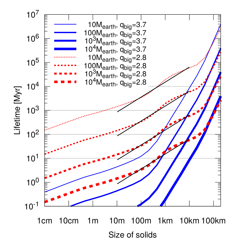
Figure 7: Collisional lifetime of bodies in two groups of fiducial debris discs (runs A and B in Appendix A). These groups assume different size distribution slopes for a primordial population of planetesimals: $q_{\mathrm{big}}=3.7$ (run A, solid blue lines) and $q_{\mathrm{big}}=2.8$ (run B, dashed red ones). Each group contains four discs with different total masses of $10M_{\oplus}$, $100M_{\oplus}$, $10^{3}M_{\oplus}$, and $10^{4}M_{\oplus}$ (lines of increasing thickness). See Appendix A for other simulation parameters. Tilted black lines are power-law fits in the $10\,\hbox{m}$ to $10\,\hbox{km}$ range, Eq. (15).

The collisional lifetimes of different-sized bodies computed in both runs (at the start of the simulations) are shown in Fig. 7. Although the total disc mass was set to the same value of $100M_{\oplus}$ in the actual ACE simulations, we also added curves for several other total masses from $10M_{\oplus}$ to $10^{4}M_{\oplus}$. This was done by using a simple fact that, for discs of different mass but with the same shape of size distributions, a collisional timescale is inversely proportional to the disc mass.

For $q_{\mathrm{big}}=3.7$ (run A), the results shown with solid lines in Fig. 7 agree with previous work (cf., e.g., Fig. 7 in Wyatt & Dent 2002, Fig. 20 in Löhne et al. 2012 or Fig. 7 in Krivov et al. 2018). They demonstrate that the size of bodies that start to be depleted after $\sim 1\,\hbox{Gyr}$ of evolution varies from several km in discs with a total mass of $10M_{\oplus}$ to about $100\,\hbox{km}$ in discs as massive as $10^{4}M_{\oplus}$. A caveat, however, is that accurate constraints on the size are difficult to get, as these depend very sensitively on the assumptions. While in Sect. 2.4 we showed that the critical fragmentation energy $Q_{\mathrm{D}}^{*}$ in the mid-size range is unimportant, outside that range it does matter. It is possible to get a much larger transition size if the km-sized and larger bodies are assumed to be particularly weak — or to collide at higher velocities. For instance, for the same Fomalhaut disc Wyatt & Dent (2002) and Quillen et al. (2007) derive $\sim 1\,\hbox{km}$ and $\sim 100\,\hbox{km}$, respectively, which traces back to different assumptions made about the strength of bodies and the different approximations employed in their collisional models.

For $q_{\mathrm{big}}=2.8$ (run B, dashed lines in Fig. 7), the resulting curves at sizes smaller than several tens of km are relatively flat. This means that $s_{\mathrm{km}}$ does depend sensitively on the system’s age $T_{\mathrm{age}}$. In the size range from $10\,\hbox{m}$ to $10\,\hbox{km}$, fitting a power law to this dependence gives

$${T_{\mathrm{age}}\over 1\,\hbox{Gyr}} = 4.17\left(s_{\mathrm{km}}\over 1\,\hbox{km}\right)^{0.625}\left(M_{\mathrm{disc}}\over 100M_{\oplus}\right)^{-1}$$ (15)

$$\times \left(M_{\star}\over M_{\odot}\right)^{-1.33}\left(R\over 100\,\hbox{au}\right)^{4.33},$$

where, apart from the $M_{\mathrm{disc}}$ scaling explained above, we have also included a $\propto R^{13/3}$ radius dependence and a $\propto M_{\star}^{-4/3}$ dependence of the collisional timescale (Wyatt et al. 2007; Löhne et al. 2008). This gives

$${s_{\mathrm{km}}\over 1\,\hbox{km}} = 0.102\left(T_{\mathrm{age}}\over 1\,\hbox{Gyr}\right)^{1.60}\left(M_{\mathrm{disc}}\over 100M_{\oplus}\right)^{1.60}$$ (16)

$$\times \left(M_{\star}\over M_{\odot}\right)^{2.13}\left(R\over 100\,\hbox{au}\right)^{-6.93}.$$

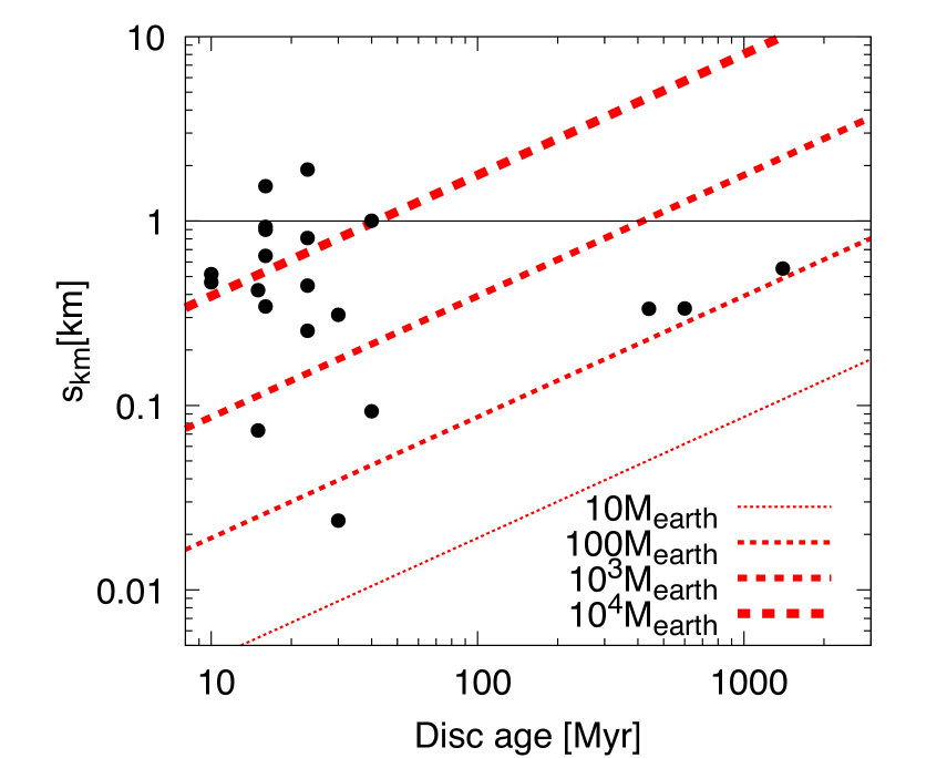
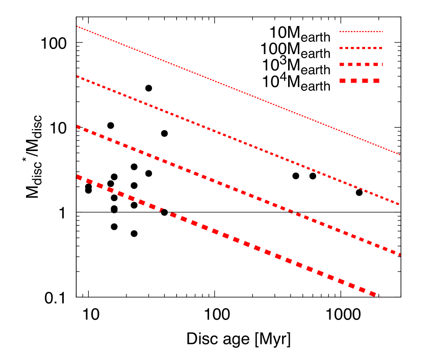
Figure 8: $s_{\mathrm{km}}$ (top) and $M_{\mathrm{disc}}^{*}/M_{\mathrm{disc}}$ (bottom) as a function of disc’s age. Lines of increasing thickness correspond to different $M_{\mathrm{disc}}$: $10M_{\oplus}$, $100M_{\oplus}$, $10^{3}M_{\oplus}$, and $10^{4}M_{\oplus}$. Points represent the 20 discs of our sample (without the Kuiper belt).

We now denote by $M_{\mathrm{disc}}$ the disc mass calculated from Eq. (9) by assuming $s_{\mathrm{km}}=1\,\hbox{km}$, and by $M_{\mathrm{disc}}^{*}$ the disc mass that we would get from the same equation if we took the “correct” $s_{\mathrm{km}}$ from Eq. (16). From Eq. (9), we obtain

$${M_{\mathrm{disc}}^{*}\over M_{\mathrm{disc}}}=\left(s_{\mathrm{km}}\over 1\,\hbox{km}\right)^{q_{\mathrm{big}}-q_{\mathrm{med}}}=\left(s_{\mathrm{km}}\over 1\,\hbox{km}\right)^{-0.9}.$$ (17)

Substituting here Eq. (16) (where $M_{\mathrm{disc}}$ is replaced by $M_{\mathrm{disc}}^{*}$) results in

$${M_{\mathrm{disc}}^{*}\over M_{\mathrm{disc}}} = 7.81\left(T_{\mathrm{age}}\over 1\,\hbox{Gyr}\right)^{-1.44}\left(M_{\mathrm{disc}}^{*}\over 100M_{\oplus}\right)^{-1.44}$$ (18)

$$\times \left(M_{\star}\over M_{\odot}\right)^{-1.92}\left(R\over 100\,\hbox{au}\right)^{-6.24}.$$

Solving this for $M_{\mathrm{disc}}^{*}$ gives

$${M_{\mathrm{disc}}^{*}\over 100M_{\oplus}} = 2.32\left(T_{\mathrm{age}}\over 1\,\hbox{Gyr}\right)^{-0.59}\left(M_{\mathrm{disc}}\over 100M_{\oplus}\right)^{0.41}$$ (19)

$$\times \left(M_{\star}\over M_{\odot}\right)^{-0.79}\left(R\over 100\,\hbox{au}\right)^{2.56}.$$

For any disc with a mass $M_{\mathrm{disc}}$ (estimated with $s_{\mathrm{km}}=1\,\hbox{km}$), having a certain age $T_{\mathrm{age}}$, Eq. (19) allows us to find the corrected mass $M_{\mathrm{disc}}^{*}$, and from Eq. (16) (using $M_{\mathrm{disc}}^{*}$ instead of $M_{\mathrm{disc}}$ there) we then find the actual transition size $s_{\mathrm{km}}$.

Lines in Fig. 8 show the results as a function of the disc age for different $M_{\mathrm{disc}}$. Overplotted with points are the individual discs in our sample. The figure demonstrates that for nearly all discs in our sample, $s_{\mathrm{km}}$ is within a factor of several of the reference value, $1\,\hbox{km}$, and $M_{\mathrm{disc}}^{*}/M_{\mathrm{disc}}$ is close to unity, within a factor of a few as well. The largest deviation of the mass ratio from unity, by a factor of 30, occurs for the young and large disc of HR 8799. The same is seen from Table 1 where both $M_{\mathrm{disc}}$ and corrected disc masses $M_{\mathrm{disc}}^{*}$ computed with Eq. (19) are given.

This means, in particular, that assuming a younger “collisional age” for a certain disc would not lead to a much lower disc mass. This is easy to understand from the above equations that are “self-regulating.” A younger collisional age means, according to Eq. (16), a smaller $s_{\mathrm{km}}$. A smaller $s_{\mathrm{km}}$ would imply a larger disc mass (see Eq. 17), but a larger mass would make $s_{\mathrm{km}}$ larger. This also explains why the scatter of $s_{\mathrm{km}}$ and $M_{\mathrm{disc}}^{*}/M_{\mathrm{disc}}$ is moderate, although parameters of individual discs vary significantly (e.g., a factor of 3 difference in radius) and the dependence on some of them is strong (such as $s_{\mathrm{km}}\propto R^{-6.93}$ as seen from Eq. 16).

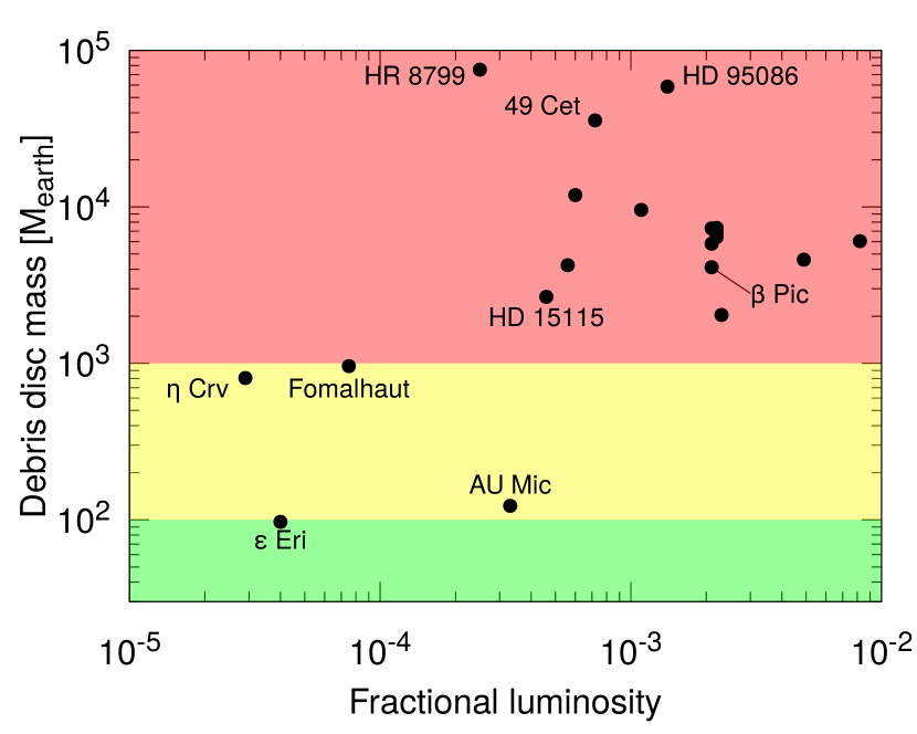
Figure 9: Similar to Fig. 5, but presenting the disc mass $M_{\mathrm{disc}}^{*}$, i.e., the total disc mass corrected for the time evolution of the transition size $s_{\mathrm{km}}$ (Eq. 20). Note that the plotting range is different from previous figures. Kuiper belt is not included.

Inserting $M_{\mathrm{disc}}$ from Eq. (9) with $s_{\mathrm{mm}}=1\,\hbox{mm}$ and $s_{\mathrm{km}}=1\,\hbox{km}$ into Eq. (19) yields

$${M_{\mathrm{disc}}^{*}\over 100M_{\oplus}} = 18.2\left(T_{\mathrm{age}}\over 1\,\hbox{Gyr}\right)^{-0.59}\left(M_{\mathrm{d}}\over M_{\oplus}\right)^{0.41}$$ (20)

$$\times \left(M_{\star}\over M_{\odot}\right)^{-0.79}\left(R\over 100\,\hbox{au}\right)^{2.56}$$

$$\times \left(s_{\mathrm{max}}\over 200\,\hbox{km}\right)^{0.49}.$$

This equation is our final estimate of the total mass obtained by extrapolating the dust masses to objects of size $s_{\mathrm{max}}$. Figure 9 plots the total disc mass $M_{\mathrm{disc}}^{*}$ for $s_{\mathrm{max}}=200\,\hbox{km}$. The majority of discs have masses between $10^{3}M_{\oplus}$ and $10^{4}M_{\oplus}$, and three discs (49 Cet, HD 95086 and HR 8799) are even more massive than $3\times 10^{4}M_{\oplus}$, or $0.1M_{\odot}$, clearly exceeding the maximum possible mass of a debris disc (Sect. 2.2).

3.4 Recent giant impacts?

Another way the disc could appear young is if the debris was created in the recent collisional disruption of an embryo-sized embedded body. It is indeed possible that such events are responsible for prominent asymmetries seen at large separations in some debris discs, such as that of $\beta$ Pictoris (Jackson et al. 2014). However, it is extremely unlikely that bright discs themselves are produced by giant impacts. There are two arguments that speak against this. Firstly, the resulting dust disc, as long as it is bright enough, will be asymmetric. That asymmetry is associated with the collision point and lasts for around $1000$ orbital periods, i.e., a few Myr at about $100\,\hbox{au}$. This is incompatible with a smooth, featureless spatial distribution of dust typically seen in (sub)mm observations of the bright discs. And conversely, at later times when the debris ring left after a giant impact becomes symmetric, it is no longer bright.

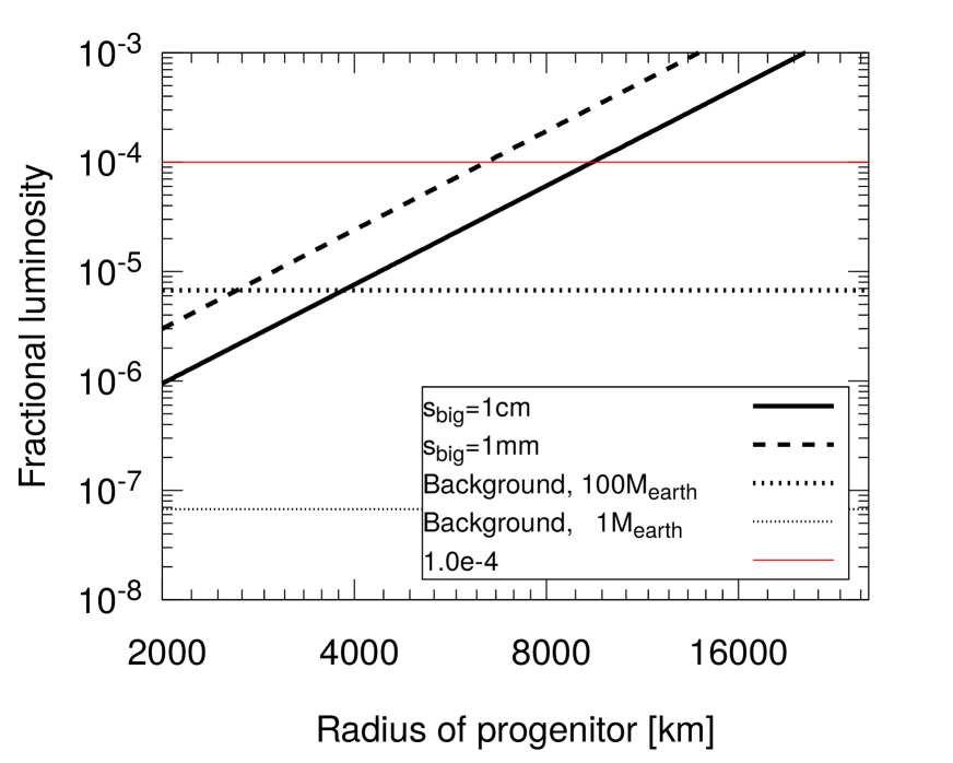
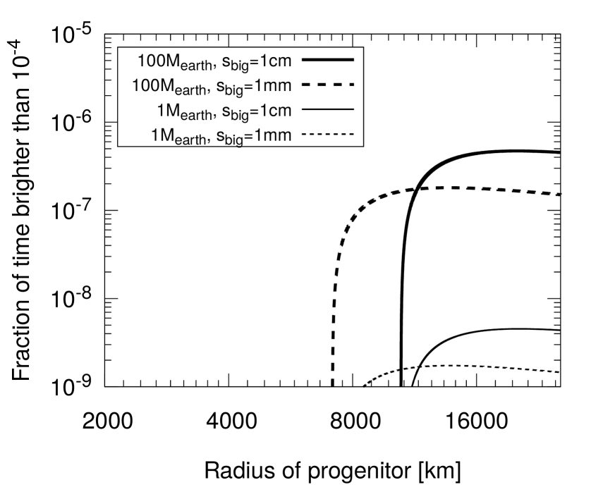
Figure 10: Brightening of debris discs by giant impacts. Top: peak fractional luminosity of the impact-generated debris cloud (slanted lines) and of the background “regular” disc (black horizontal lines). Bottom: fraction of time during which the impact debris has a fractional luminosity greater than $10^{-4}$. Thick lines: $M_{\mathrm{disc}}=100M_{\oplus}$, thin: $M_{\mathrm{disc}}=1M_{\oplus}$. Solid lines: $s_{\mathrm{big}}=10\,\hbox{cm}$, dashed: $s_{\mathrm{big}}=1\,\hbox{mm}$.

Secondly, it is easy to show the frequency of such events is too low. We consider an underlying debris disc of mass $M_{\mathrm{disc}}$ in particles with radii [$s_{\mathrm{blow}}$, $s_{\mathrm{max}}$] (with $s_{\mathrm{blow}}$ being the blowout size), in which a big object (“progenitor”) of radius $s_{\mathrm{p}}$ (mass $M_{\mathrm{p}}$) is collisionally disrupted, releasing a fraction $\alpha$ of its mass into grains with radii [$s_{\mathrm{blow}}$, $s_{\mathrm{big}}$]. We assume, for simplicity, the size distribution of particles both in the background disc and the impact-generated debris cloud to follow the Dohnanyi law with $q=3.5$. Both the fractional luminosity of the background disc $f_{\mathrm{bkg}}$ and that of the debris cloud $f_{\mathrm{cl}}$ are calculated from Eq. (15) of Wyatt (2008) showing, in particular, that

$$f_{\mathrm{cl}}\propto M_{\mathrm{p}}s_{\mathrm{big}}^{-0.5}.$$ (21)

The ratio of the two luminosities is given by

$${f_{\mathrm{cl}}\over f_{\mathrm{bkg}}}={\alpha M_{\mathrm{p}}\over M_{\mathrm{disc}}}\left(s_{\mathrm{max}}\over s_{\mathrm{big}}\right)^{0.5},$$ (22)

and so the collisional debris can only be brighter than the background disc if a single progenitor holds a significant fraction of the total mass, and the collisional debris is put into small particles.

For the same set of stellar and disc parameters as in Appendix A and assuming $\alpha=0.03$ (as in Jackson et al. 2014), the fractional luminosities are depicted in Fig. 10 (top) for different values of $M_{\mathrm{disc}}$ and $s_{\mathrm{big}}$. The figure shows that the debris cloud can only have fractional luminosity in excess of $f_{\mathrm{lim}}\equiv 10^{-4}$ (shown with thin red line) if the progenitor is larger than $\sim 7000$–$10000\,\hbox{km}$ in size, depending on the $\,\hbox{s}_{\mathrm{big}}$ assumed. This threshold value of $10^{-4}$ was chosen because it roughly corresponds to the fractional luminosity above which most of the discs are affected by the mass problem, see Fig. 5.

The timescale $T_{\mathrm{p}}$, on which the progenitor gets disrupted in the disc, is given by Eq. (16) of Wyatt (2008). The timescale $T_{\mathrm{cl}}$ on which the debris cloud decays with time (considering only mutual collisions rather than with the background disc as we require $f_{\mathrm{cl}}>f_{\mathrm{bkg}}$) can also be computed from Eq. (16) of Wyatt (2008). Thus the ratio of the two timescales is

$${T_{\mathrm{cl}}\over T_{\mathrm{p}}}={M_{\mathrm{disc}}\over\alpha M_{\mathrm{p}}}\left(s_{\mathrm{big}}\over s_{\mathrm{p}}\right)\left(s_{\mathrm{p}}\over s_{\mathrm{max}}\right)^{0.5}=\left(f_{\mathrm{bkg}}\over f_{\mathrm{cl}}\right)\left(s_{\mathrm{big}}\over s_{\mathrm{p}}\right)^{0.5}.$$ (23)

The fractional luminosity of the collisional debris evolves as $f_{\mathrm{cl}}/(1+t/T_{\mathrm{cl}})$ (see Eq. 17 of Wyatt 2008), and so the time it spends above $f_{\mathrm{lim}}=10^{-4}$ is $T_{\mathrm{cl}}(f_{\mathrm{cl}}/f_{\mathrm{lim}}-1)$. Thus the fraction of time for which the aftermath of a giant collision will have a fractional luminosity larger than $10^{-4}$, is given by $(T_{\mathrm{cl}}/T_{\mathrm{p}})(f_{\mathrm{cl}}/f_{\mathrm{lim}}-1)$, and $T_{\mathrm{cl}}/T_{\mathrm{p}}$ from Eq. (23) is a good estimate of the fraction of time collisional debris from a single disruption event should remain detectable. It is the last equality in Eq. (23) that leads to the conclusion that collisional debris that is detectable above the background disc must be rare, since by definition $f_{\mathrm{bkg}}/f_{\mathrm{cl}}<1$ and so the only way of not making this rare is to have a large $s_{\mathrm{big}}$, but Eq. (21) shows that a large $s_{\mathrm{big}}$ would result in small $f_{\mathrm{cl}}$ and Eq. (22) that this would also make it harder to achieve $f_{\mathrm{cl}}/f_{\mathrm{bkg}}>1$.

This fraction of time over which a disc has $f_{\mathrm{cl}}>10^{-4}$ is plotted in Fig. 10 bottom. A disc enhanced by impact-generated debris can only be sufficiently bright for a non-negligible fraction of its age if the background disc is massive (otherwise giant impacts are too rare and/or sufficiently large progenitors are absent), the disrupted progenitor is large (otherwise the amount of the injected debris is too low), and the largest fragment is large enough (otherwise the debris cloud decays too fast). However, even in the most favourable case of those considered (massive disc with $M_{\mathrm{disc}}\sim 100M_{\oplus}$, an Earth-sized progenitor with $s_{0}\sim 10^{4}\,\hbox{km}$, boulder-sized largest debris fragment with $s_{\mathrm{big}}\sim 1\,\hbox{cm}$), the fraction of time when the disc is bright does not exceed $\sim 10^{-6}$. This fraction of time is far too small to explain all those discs that require an unrealistically high mass, since about 20 percent of all stars have detectable debris discs (Eiroa et al. 2013; Thureau et al. 2014; Montesinos et al. 2016; Sibthorpe et al. 2018), and about one-fourth or one-third of them are affected by the mass problem.

3.5 “Planetesimals born small”?

For planetesimals with a flat primordial distribution, the discussion in Sect. 3.3 and the collisional lifetimes plotted in Fig. 7 (with dashed lines) make it clear that bodies larger than a kilometre in size are not part of the collisional cascade even in old systems, making only a minor contribution to the observed dust production through cratering collisions with much smaller projectiles. As a result, setting the maximum size in collisional models to $\sim 1\,\hbox{km}$ is sufficient to reproduce the observed discs. In other words, large bodies are not required at all by collisional models. However, since the disc mass is proportional to $s_{\mathrm{max}}^{4-q}$, and $q=q_{\mathrm{big}}=2.8$ at $s\ga 1\,\hbox{km}$, replacing $s_{\mathrm{max}}=200\,\hbox{km}$ with $s_{\mathrm{max}}=1\,\hbox{km}$ would reduce the total disc mass by a factor of $600$!

To see how this applies to the discs in our sample, we note that time-dependent size $s_{\mathrm{km}}$ given by Eq. (16) serves as a reasonable estimate for the size of the bodies that feed the cascade in these discs, given their age. A caveat is that a derivation of $s_{\mathrm{km}}$ in Sect. 3.3 assumed the flat primordial distribution. Yet its presence does not alter collisional lifetimes of km-sized objects markedly, so that a calculation neglecting the bodies larger than kilometres would not change $s_{\mathrm{km}}$ more than by a factor of a few. This size, which is plotted in Fig. 8 (top) and listed in Table 1, ranges from $\approx 0.1\,\hbox{km}$ to $\approx 7\,\hbox{km}$. Assuming now that bodies larger than $s_{\mathrm{km}}$ were absent, the discs would have a mass

$$M_{\mathrm{disc}}^{\mathrm{min}}=M_{\mathrm{d}}\;{4-q\phantom{{}_{b}ig}\over 4-q_{\mathrm{med}}}\left(s_{\mathrm{km}}\over s_{\mathrm{mm}}\right)^{4-q_{\mathrm{med}}}.$$ (24)

This mass is given in the last column of Table 1 and ranges from $0.2M_{\oplus}$ (for the $\varepsilon$ Eri disc) to $86M_{\oplus}$ (for the HD 131488 disc). These values are within an order of magnitude consistent with “minimum disc mass” estimates in Sect. 2.1 obtained with the mass loss argument and are a way below the “maximum disc masses” discussed in Sect. 2.2. In summary, a hypothesis that large bodies for some reason do not form on the periphery of planetary systems would provide the easiest solution to the debris disc mass problem.

This conclusion is also robust with respect to a possible uncertainty in the assumed slope $q_{\mathrm{med}}$. This is because $s_{\mathrm{km}}$ in Eq. (24) also depends on $q_{\mathrm{med}}$ in such a way that $M_{\mathrm{disc}}^{\mathrm{min}}$ is independent of $q_{\mathrm{med}}$. Indeed, for any size distribution with a single slope $3<q_{\mathrm{med}}<4$ that is in steady state, the collisional lifetime of an object of size $s$ is $T_{\mathrm{coll}}(s)=T_{\mathrm{coll}}(s_{\mathrm{mm}})(s/s_{\mathrm{mm}})^{4-q_{\mathrm{med}}}$ (see, e.g., Eq. 36 in Wyatt et al. 2011). Since $s_{\mathrm{km}}$ should satisfy the equation $T_{\mathrm{coll}}(s_{\mathrm{km}})=T_{\mathrm{age}}$, we find $(s_{\mathrm{km}}/s_{\mathrm{mm}})=[T_{\mathrm{age}}/T_{\mathrm{coll}}(s_{\mathrm{mm}})]^{1/(4-q_{\mathrm{med}})}$. Substituting this into Eq. (24) shows that $M_{\mathrm{disc}}^{\mathrm{min}}$ is independent of $q_{\mathrm{med}}$ in the single-slope approximation. In fact, the conclusion that $M_{\mathrm{disc}}^{\mathrm{min}}$ is independent of $q_{\mathrm{med}}$ is more general and only relies on the assumption of steady state. This is because in steady state the mass loss rate from the top end of the cascade ($M_{\mathrm{disc}}^{\mathrm{min}}/T_{\mathrm{age}}$) is equal to that at the small size end ($M_{\mathrm{d}}/T_{\mathrm{coll}}(s_{\mathrm{mm}})$). The derived $M_{\mathrm{disc}}^{\mathrm{min}}$ is thus completely independent of the size distribution above $s_{\mathrm{mm}}$.

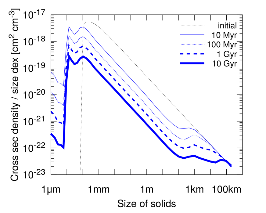
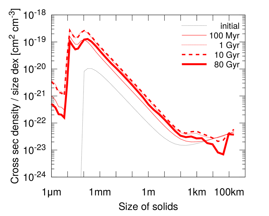
Figure 11: Long-term evolution of the size distribution in two fiducial debris discs of $100M_{\oplus}$ (Appendix A), assuming different size distribution slopes for a primordial population of planetesimals: $q_{\mathrm{big}}=3.7$ (run A, top panel) and $q_{\mathrm{big}}=2.8$ (run B, bottom). Black dotted line: initial distributions. Coloured lines of increasing thickness: distributions at later times, as indicated in the legends.

The above discussion makes it obvious that, if the bodies larger than $s_{\mathrm{km}}$ were absent, the mass problem would not arise. There is also an argument against the presence of a primordial population of planetesimals with a relatively flat size distribution from the fact that such a primordial distribution results in dust mass that increases with age. Given the three-phase size distribution discussed in Sect. 2.4, with $s_{\mathrm{km}}$ increasing with age as in Sect. 3.3, this increase of dust mass with age occurs whenever $q_{\mathrm{big}}<q_{\mathrm{med}}$, and continues until the largest planetesimals reach collisional equilibrium. This behaviour is reproduced in the numerical simulations of the size distribution (run B in Appendix A), which show that while a three-phase distribution is an approximation, there is still an increase in dust mass until $\sim 10\,\hbox{Gyr}$ (Fig. 11 bottom). This contradicts observations, as there is ample evidence for a long-term decay in the dust mass in debris discs (e.g., Zuckerman & Becklin 1993; Habing et al. 1999, 2001; Spangler et al. 2001; Greaves & Wyatt 2003; Rieke et al. 2005; Moór et al. 2006; Eiroa et al. 2013; Chen et al. 2014; Moór et al. 2015; Holland et al. 2017; Sibthorpe et al. 2018).

We note that collisional equilibrum at large sizes is reached, and so the dust mass starts to decay, on much shorter timescales in smaller discs. For instance, Nesvorný & Vokrouhlický (2019) did a collisional simulation for a primordial Kuiper belt of $40M_{\oplus}$ at around $\sim 25\,\hbox{au}$ with an initial size distribution from streaming instability simulations, similar to our run B in Appendix A. They found that collisional equilibrium is achieved by bodies of up to $50\,\hbox{km}$ in radius in just $\sim 50\,\hbox{Myr}$. Equation (15) suggests that the collisional timescale scales as $M_{\mathrm{disc}}^{-1}M_{\star}^{-1.33}R^{4.33}$. Thus, if our run B gave $\sim 10\,\hbox{Gyr}$ for $200\,\hbox{km}$-sized planetesimals in a $100M_{\oplus}$ disc with a radius of $100\,\hbox{au}$ around a $2.16M_{\odot}$ star, then same-sized bodies in the Kuiper belt would reach equilibrium at $\sim 170\,\hbox{Myr}$. For $50\,\hbox{km}$-sized bodies, the timescale would be even shorter, consistent with their result. What this means is that large planetesimals may still be required (i.e., $s_{\mathrm{km}}\gg 1\,\hbox{km}$) to replenish the dust in discs with small radii found around old stars. Moreover, for small discs it may be concluded for old stars that the level of dust observed is incompatible with steady state erosion regardless of the size of their planetesimals (e.g., Wyatt et al. 2007).

To make the dust mass decrease in time for all discs regardless of their radius, we have to admit that the primordial population has a sufficiently steep size distribution (as in run A of Appendix A, see Fig. 11 top). To find out what “sufficiently steep” means, we note that the slope $q_{\mathrm{med}}$ flattens from $3.7$ for objects smaller than $\sim 0.1\,\hbox{km}$ that reside in the strength regime (as predicted by Eq. 11 with $\gamma=-0.37$ and $p=0$) to $3.0$ for larger objects that are in the gravity regime (where $\gamma=1.38$). It is the latter value that determines how steep the primordial size distribution of planetesimals has to be in order not to cause the long-term increase in the amount of dust that contradicts the observations. In other words, for the debris disc brightness to decrease with time as observed, this requires the initial size distribution of mass-dominating large planetesimals to be steeper than $q_{\mathrm{big}}=3.0$.

To solve the disc mass problem, we also need the size distribution to be such that the ratio of the total mass to the mass in km-sized objects (i.e., the largest objects in the primordial population that are small enough to experience catastrophic collisions on timescales shorter than the system ages) is not too large. This can be achieved either by a very steep distribution ($q_{\mathrm{big}}>4$ to put the mass in the smallest objects) or for the largest planetesimals to be smaller than assumed. While the idea that large planetesimals are nearly or completely absent in bright debris discs would help solve the mass problem and would remove any possible tension with the observed statistics of different-aged discs, it comes with several caveats. One is that rapid and efficient formation of planetesimals as big as hundreds of kilometres is robustly predicted by certain models of planetesimal formation. For instance, Schäfer et al. (2017) predict the top-end of the initial mass distribution to be exponentially tapered at masses $\sim 10^{-5}G^{-1}H_{\mathrm{g}}^{3}P^{-2}$ (with $G$ being the gravitational constant and $H_{\mathrm{g}}$ the scale height of gas in a protoplanetary disc). For a broad range of plausible parameters, this corresponds to sizes on the order of hundreds of kilometres. Nevertheless, many aspects of planetesimal formation are not yet fully understood. It appears possible that state-of-the-art models might still miss some essential pieces of physics or that some of the underlying assumptions fail in reality.

Another concern about the suggested scarcity of $>1\,\hbox{km}$ bodies in debris discs might be the fact that our own Kuiper belt is populated by numerous transneptunian objects $\sim 100\,\hbox{km}$ in size. While Kuiper-belt objects (KBOs) in the dynamically hot populations (hot classicals, scattered disc objects) must have formed closer in $<30\,\hbox{au}$ and were implanted in the present-day Kuiper belt by the migration of Neptune, there is ample evidence that the cold classical KBOs accreted in-situ at their current location between $42$–$48\,\hbox{au}$ (see Morbidelli & Nesvorný 2020, and references therein). This conclusion is strongly backed up, for instance, by a high fraction of equal-sized binaries in this population (e.g., Nesvorný & Vokrouhlický 2019). Thus we do know that planetesimals with $\sim 100\,\hbox{km}$ in size formed successfully at the periphery of our Solar system. Their inferred size distribution between a few km and $\sim 50$–$100\,\hbox{km}$ is flat ($q_{\mathrm{big}}\sim 3$), in good agreement with planetesimal formation model predictions. Above $\sim 50$–$100\,\hbox{km}$, the distribution steepens drastically to $q_{\mathrm{big}}\ga 6$ (Bernstein et al. 2004), so that the largest cold classicals such as (119951) 2002 KX14 with $s\sim 200\,\hbox{km}$ (Vilenius et al. 2012) make a negligible contribution to the total mass. Nevertheless, these facts are only valid for our own Solar system (which is not a system with a disc mass problem), and we do not know whether it is representative of other planetary systems. Given the bewildering diversity of extrasolar planets discovered so far, it is quite possible that circumstances and outcomes of planetesimal formation also vary significantly from one system to another.

4 Discussion

4.1 A possible “big picture”

The above analysis points to a conclusion that large planetesimals should be absent in systems with bright debris discs. This implies that planetesimal formation processes yield different-sized planetesimals in some systems. The reasons for that are not known, but they could be related to the conditions in the protoplanetary discs. It is also possible that the efficiency of planetesimal formation, i.e., the fraction of available mass that is turned into planetesimals of some size, could be different for the formation of smaller versus larger planetesimals.

A visual inspection of plots such as Fig. 5 suggests that the total mass of debris discs, inferred under an assumption of $s_{\mathrm{max}}$ being the same for all discs, shows a monotonic rise with fractional luminosity. One hypothesis could be that the true total mass in all the discs is comparable but, for some reasons, the largest planetesimals in brighter discs are smaller. Indeed, Eq. (9) tells us the inferred total mass is proportional to $M_{\mathrm{d}}s_{\mathrm{max}}^{4-q_{\mathrm{big}}}$, where $M_{\mathrm{d}}\propto f_{\mathrm{d}}$. Were $s_{\mathrm{max}}\propto f_{\mathrm{d}}^{-1/(4-q_{\mathrm{big}})}\propto f_{\mathrm{d}}^{-0.8}$, the total mass of all discs would be similar. To give a numerical example, all bright discs with fractional luminosities in the range from $10^{-4}$ to $10^{-2}$ could have approximately the same mass $M_{\mathrm{disc}}\sim 100M_{\oplus}$, if the radius of the biggest planetesimals varied from $\sim 200\,\hbox{km}$ at $f_{\mathrm{d}}=10^{-4}$ to $\sim 4\,\hbox{km}$ at $f_{\mathrm{d}}=10^{-2}$.

In other words, it can be that all protoplanetary discs leave behind a comparable mass in small bodies by the time of gas dispersal, yet the ability to form the largest objects varies from one system to another. In that case, the brightest debris discs would form in those systems where the planetesimals have smaller, kilometre sizes. And conversely, fainter debris discs would emerge in those systems where planetesimals hundreds of kilometres in radius succeeded to form.

Our present-day Kuiper belt would be exempt from this trend, as its total mass is much lower than that of the (currently detectable) extrasolar discs. The likely reason for that is early depletion of the primordial Kuiper belt by a dynamical instability of giant planets (e.g., Morbidelli & Nesvorný 2020). Without that event, the $\sim 30M_{\oplus}$ debris disc of the Solar system would have been comparable in brightness with the brightest known extrasolar discs in terms of its $24$ $\mu$m and $70$ $\mu$m emission (see Fig. 12 in Booth et al. 2009). This may appear incompatible with the above argument in which a bright primordial Kuiper belt might be taken to infer that it was born with small planetesimals, whereas these models include bodies up to $500\,\hbox{km}$ in radius. However, the primordial Kuiper belt’s infrared emission is not inferred to be bright because its mass is concentrated in small planetesimals, rather because of its small radius ($\sim 20\ldots 30\,\hbox{au}$) and so hot temperature compared with extrasolar discs which are more typically $\sim 100\,\hbox{au}$. This underscores the importance of disc radius in the analysis, since being bright in the infrared does not necessarily indicate a mass problem if the emission is hot. Sub-mm dust mass is a better indicator of a possible disc mass problem, since by that metric the primordial Kuiper belt is one to two orders of magnitude lower than that of the brightest known debris discs (see Fig. 12 in Booth et al. 2009, for their “comet-like” dust composition).

It is also interesting that the discs that appear to be the most problematic and so need the “planetesimals born small” hypothesis, are those with the largest radii (see Fig. 6a). This suggests that the biggest planetesimals may be smaller at larger distances. This possibility might be supported by recent simulations of Klahr & Schreiber (2020), which showed that the expected typical size of planetesimals formed via the SI plunges down outside $\sim 50\,\hbox{au}$ from the star (see their Fig. 10). Thus it is possible that more compact discs, such as the Kuiper belt, succeeded to form larger planetesimals, whereas many of the well known extrasolar discs, being much larger, have a size distribution limited to smaller ones.

Of course, there is no requirement for all stars to have discs with the same mass. Just as the Kuiper belt is lower in mass because of some level of depletion, so too could the $f_{\mathrm{d}}=10^{-4}$ discs simply be lower in mass, either because they formed less massive, or because they suffered some depletion. As a numerical example, an $f_{\mathrm{d}}=10^{-4}$ disc could have a total mass as low as $M_{\mathrm{disc}}\sim 1M_{\oplus}$, if the biggest planetesimals were as small as $\sim 4\,\hbox{km}$ in radius.

4.2 Implications

One immediate implication of having fewer large planetesimals in debris discs would be that these discs are not self-stirred (Kenyon & Bromley 2008; Kennedy & Wyatt 2010; Krivov & Booth 2018). For instance, the presence of $\ga 400\,\hbox{km}$-sized embedded bodies is required to self-stir the AU Mic disc (Daley et al. 2019), and at least $\sim 100\,\hbox{km}$-sized planetesimals are necessary to reproduce the stirring level of the dynamically cold population recently discovered in the $\beta$ Pic disc (Matrà et al. 2019). However, there are possibilities other than self-stirring to explain the inferred excitation level of planetesimals in debris discs. Alternative mechanisms include stirring by planets near the inner edges of the discs (Quillen 2006) or elsewhere in the disc cavities (Mustill & Wyatt 2009) or “‘primordial” excitation of planetesimals forming in self-gravitating protoplanetary discs (Walmswell et al. 2013).

A lack of big planetesimals would also affect planetesimal-driven migration of planets in the systems, which is known to be a viable mechanism to explain structure in our Kuiper belt (Malhotra 1995) and extrasolar debris discs (Wyatt 2003). Migration, which otherwise has a stochastic component (Zhou et al. 2002), would become smoother in the absence of large bodies (Chiang et al. 2003). This would make resonant trapping of planetesimals easier, perhaps helping to explain some of the observed features in the discs such as the $\beta$ Pictoris clump (Dent et al. 2014).

Should the systems with bright debris discs indeed be dominated by small (km-sized) planetesimals, this would necessitate revisions to the existing planetesimal formation models. Perhaps this could also help constrain conditions in the PPDs and how they vary from one system to another. Strictly speaking, our conclusion only applies to the outer region (outside 10s to  au) that is currently occupied by debris-producing residual planetesimals. It is not clear if the planetesimal formation that happens at large distances is similar to what is going on closer in. If so, this would have profound implications for planet formation theories (e.g., growth to embryos and full-size planets). Specifically, this would pose a challenge of how to build inner planets — which we know to exist in many systems – starting from planetesimals of smaller sizes (see a discussion in Voelkel et al. 2020, and references therein).

4.3 Potential tests

Are there any ways to constrain either the sizes of the largest planetesimals, the total masses of debris discs, or both? In principle information on the largest planetesimals is encoded in the statistics of debris disc detections as a function of age. Population models which follow the erosion of planetesimal belts as they deplete through collisions have been able to reproduce these statistics (e.g., Wyatt et al. 2007; Löhne et al. 2008; Gáspár et al. 2013). However, they have yet to set strong constraints on the largest planetesimal size or disc mass, since the collisional depletion timescale in such models is degenerate with the level of stirring and planetesimal strength for example. The distribution of planetesimal belt radii is also very uncertain when inferring this from the emission spectrum, which is another important parameter in determining collisional lifetimes. High resolution imaging is improving constraints on stirring levels (e.g., Daley et al. 2019; Matrà et al. 2019) and also on planetesimal belt radii which may correlate with stellar luminosity (Matrà et al. 2018). This means that we can hope that constraints on parameters such as the size of the largest planetesimals will soon be possible. For example, it can be expected that discs in which the planetesimals are born small would appear bright at young ages (10s of Myr) then rapidly decay (e.g., within a few 100 Myr), whereas those in which planetesimals are born large would start out fainter, but maintain that brightness at a relatively constant level over several Gyr. Thus it may be possible to find signatures of the largest planetesimal size in comparative studies of populations in the 10Myr–Gyr range.

As far as measuring disc mass is concerned, one possibility is to use the observed disc structure as an indicator of disc mass. For example, if the disc is massive enough for its self-gravity to become important, this could affect the structure of the disc (Sefilian & Wyatt, in prep.). Besides, planet-disc interaction should result in different dynamical patterns, depending on whether the disc mass is lower or comparable to that of the planet (Pearce & Wyatt 2014, 2015). For instance, in the latter case a single planet in eccentric orbit could explain a double-ringed structure of a debris disc exterior to the planet’s orbit, such as the one observed in HD 107146 (Marino et al. 2018) and HD 92945 (Marino et al. 2019). In the former case, the same structure could rather be attributed to a planet in a nearly-circular orbit between the two rings and clearing its orbit from debris. Thus finding planets in one of those systems would help indirectly “measure” the disc mass, depending on the orbit and mass of the planet discovered. Finally, a disc’s mass would also affect how far and how fast (Neptune-mass) planets migrate through planetesimal scattering, which may have observable consequences (see, e.g., Sect. 4.3 in Marino et al. 2018, for a detailed discussion).

5 Conclusions

In this paper, we consider the total mass of debris discs and how it is related to the overall mass budget of solid material in planetary systems. Since the disc mass is dominated by directly unobservable planetesimals, it has to be estimated from the mass of debris dust produced in their collisions. That dust mass is inferred from (sub)mm observations, assuming a certain opacity. The dust mass is then extrapolated to the mass of planetesimals up to a certain size, using theoretical models of a dust-producing collisional cascade.

The total disc mass found in this way must satisfy certain constraints that we define as follows. The “minimum debris disc mass”, which is needed to collisionally sustain the debris dust at the observed level over the system’s age, is estimated to be $\sim 10M_{\oplus}$. The “maximum debris disc mass” is determined by the total mass of condensible compounds that are available in protoplanetary discs out of which debris discs and planets formed. This should be of the order of $\sim 100$…$1000M_{\oplus}$.

Estimating the dust mass for a sample of 20 bright debris discs with reliable ALMA (sub)mm fluxes, and extrapolating up to the $200\,\hbox{km}$-sized planetesimals, we find the total disc mass to lie in the $\sim 10^{3}$…$10^{4}M_{\oplus}$ range for the majority of discs in the sample, which clearly exceeds the maximum possible mass. We refer to this as a “debris disc mass problem.”

In an attempt to resolve the controversy, we re-analyse possible uncertainties as well as the various assumptions made in estimating the disc mass. For instance, the dust mass is uncertain by a factor of several, because so is the assumed dust opacity. It is also possible that collisional damping and damping by secondary gas steepen the size distribution somewhat, although we find these processes to be inefficient. Next, if the bodies are weaker than assumed (which increases the size of the bodies that start to be depleted by the age of the systems), the estimated total disc mass will reduce by a factor of several. If the density of larger bodies is lower than that of smaller ones, this will also result in a several times smaller disc mass estimate. None of the factors like these, taken alone, would solve the mass problem. However, it cannot be ruled out that several of them in combination would mitigate the tension between the estimated and maximum possible debris disc masses, although probably not providing an ultimate solution to the problem.

We argue that the easiest solution to the mass problem would be to admit that the size of the largest planetesimals in bright discs is of the order of kilometres, and thus smaller than might be expected given the size distribution of planetesimals in the Solar system and current planetesimal formation models. It is possible that the largest planetesimals formed farther out from the star have smaller sizes, so that compact discs such as our Kuiper belt are dominated by large planetesimals, while larger discs have a size distribution limited to small planetesimals. The size of the biggest bodies may also vary strongly from one system to another, such that the systems where planetesimal accretion far from the star stalled at smaller sizes formed the brightest debris discs. This “planetesimals born small” scenario would set important constraints on the planetesimal formation processes from the debris disc perspective. It would also have a number of implications for planetesimal-driven migration and growth of planetary cores and planets.

Data availability

The data underlying this article will be shared on reasonable request to the corresponding author.

Appendix A Collisional simulations

In this Appendix, we describe two simulations with the ACE code (e.g., Krivov et al. 2013) which we refer to throughout the paper:

• Run A. The setup included a $10\,\hbox{au}$ wide ring of planetesimals around a distance of $100\,\hbox{au}$. As a central star, we chose an A-type star of $2.16$ solar masses with a luminosity of $27.7$ times the solar one. For planetesimals smaller than $1\,\hbox{km}$, we took the initial size distribution with a slope $q_{\mathrm{med}}=3.7$. The largest planetesimals were assumed to have $200\,\hbox{km}$ in radius, and the initial size distribution slope of the primordial population of objects with radii from $1\,\hbox{km}$ to $200\,\hbox{km}$ was set to $q_{\mathrm{big}}=3.7$, i.e., made the same as for sub-km planetesimals. The total disc mass was set to $100M_{\oplus}$. The planetesimals were assumed to have a distribution of eccentricities between 0 and 0.1 and inclinations from 0 to 3 degrees. As material, we took a mixture of astrosilicate (Draine 2003) and water ice (Li & Greenberg 1998) in equal volume fractions with a bulk density of $\rho=2.35\,\hbox{g}\,\hbox{cm}^{-3}$. A number of other standard assumptions were also made (see Krivov et al. 2018, for a complete list of parameters assumed).

  Results of run A are shown in Fig. 1 (a typical simulated size distribution), Fig. 7 (with solid lines; collisional lifetimes), and Fig. 11 top (long-term evolution of the size distribution).

• Run B. All the parameters were taken the same as in run A, except that the assumed initial size distribution slope of the primordial population of objects with radii from $1\,\hbox{km}$ to $200\,\hbox{km}$ was set to $q_{\mathrm{big}}=2.8$, as predicted by pebble concentration models of planetesimal formation.

  Results of run B are shown in Fig. 4 (a typical simulated size distribution), Fig. 7 (with dashed lines; collisional lifetimes), and Fig. 11 bottom (long-term evolution of the size distribution).

References

- Abod et al. (2019) Abod C. P., Simon J. B., Li R., Armitage P. J., Youdin A. N., Kretke K. A., 2019, Astrophys. J., 883, 192
- Andrews et al. (2009) Andrews S. M., Wilner D. J., Hughes A. M., Qi C., Dullemond C. P., 2009, Astrophys. J., 700, 1502
- Andrews et al. (2010) Andrews S. M., Wilner D. J., Hughes A. M., Qi C., Dullemond C. P., 2010, Astrophys. J., 723, 1241
- Beckwith & Sargent (1991) Beckwith S. V. W., Sargent A. I., 1991, Astrophys. J., 381, 250
- Bernstein et al. (2004) Bernstein G. M., Trilling D. E., Allen R. L., Brown M. E., Holman M., Malhotra R., 2004, Astron. J., 128, 1364
- Bertelli et al. (1994) Bertelli G., Bressan A., Chiosi C., Fagotto F., Nasi E., 1994, A&AS, 106, 275
- Blum et al. (2017) Blum J., et al., 2017, MNRAS, 469, S755
- Booth et al. (2009) Booth M., Wyatt M. C., Morbidelli A., Moro-Martín A., Levison H. F., 2009, MNRAS, 399, 385
- Bottke et al. (2005) Bottke W. F., Durda D. D., Nesvorný D., Jedicke R., Morbidelli A., Vokrouhlický D., Levison H. F., 2005, Icarus, 179, 63
- Britt et al. (2002) Britt D. T., Yeomans D., Housen K., Consolmagno G., 2002, in Bottke Jr. W. F., Cellino A., Paolicchi P., Binzel R. P., eds, Asteroids III. University of Arizona Press, Tucson, pp 485–500
- Brown (2012) Brown M. E., 2012, Ann. Rev. Earth Planet. Sci., 40, 467
- Burns et al. (1979) Burns J. A., Lamy P. L., Soter S., 1979, Icarus, 40, 1
- Campo Bagatin et al. (1994) Campo Bagatin A., Cellino A., Davis D. R., Farinella P., Paolicchi P., 1994, Planet. Space Sci., 42, 1079
- Carrera et al. (2017) Carrera D., Gorti U., Johansen A., Davies M. B., 2017, Astrophys. J., 839, 16
- Cataldi et al. (2020) Cataldi G., et al., 2020, Astrophys. J., 892, 99
- Chambers (2010) Chambers J. E., 2010, Icarus, 208, 505
- Chen et al. (2014) Chen C. H., Mittal T., Kuchner M., Forrest W. J., Lisse C. M., Manoj P., Sargent B. A., Watson D. M., 2014, Astrophys. J. Suppl., 211, 25
- Chiang & Laughlin (2013) Chiang E., Laughlin G., 2013, MNRAS, 431, 3444
- Chiang et al. (2003) Chiang E. I., et al., 2003, Astron. J., 126, 430
- Cuzzi et al. (2008) Cuzzi J. N., Hogan R. C., Shariff K., 2008, Astrophys. J., 687, 1432
- Cuzzi et al. (2010) Cuzzi J. N., Hogan R. C., Bottke W. F., 2010, Icarus, 208, 518
- Daley et al. (2019) Daley C., et al., 2019, Astrophys. J., 875, 87
- Delbo’ et al. (2017) Delbo’ M., Walsh K., Bolin B., Avdellidou C., Morbidelli A., 2017, Science, 357, 1026
- Dent et al. (2014) Dent W. R. F., et al., 2014, Science, 343, 1490
- Dohnanyi (1969) Dohnanyi J. S., 1969, J. Geophys. Res., 74, 2531
- Dominik & Decin (2003) Dominik C., Decin G., 2003, Astrophys. J., 598, 626
- Draine (2003) Draine B. T., 2003, Ann. Rev. Astron. Astrophys., 41, 241
- Draine (2006) Draine B. T., 2006, Astrophys. J., 636, 1114
- Draine & Lee (1984) Draine B. T., Lee H. M., 1984, Astrophys. J., 285, 89
- Durda & Dermott (1997) Durda D. D., Dermott S. F., 1997, Icarus, 130, 140
- Eiroa et al. (2013) Eiroa C., et al., 2013, Astron. Astrophys., 555, A11
- Fraser et al. (2014) Fraser W. C., Brown M. E., Morbidelli A., Parker A., Batygin K., 2014, ApJ, 782, 100
- Fulle et al. (2016) Fulle M., et al., 2016, MNRAS, 462, S132
- Gáspár et al. (2013) Gáspár A., Rieke G. H., Balog Z., 2013, Astrophys. J., 768, 25
- Greaves & Rice (2010) Greaves J. S., Rice W. K. M., 2010, MNRAS, 407, 1981
- Greaves & Wyatt (2003) Greaves J. S., Wyatt M. C., 2003, MNRAS, 345, 1212
- Greaves et al. (2007) Greaves J. S., Fischer D. A., Wyatt M. C., Beichman C. A., Bryden G., 2007, MNRAS, 378, L1
- Habing et al. (1999) Habing H. J., et al., 1999, Nature, 401, 456
- Habing et al. (2001) Habing H. J., et al., 2001, Astron. Astrophys., 365, 545
- Haghighipour & Boss (2003) Haghighipour N., Boss A. P., 2003, Astrophys. J., 598, 1301
- Häßner et al. (2018) Häßner D., Mutschke H., Blum J., Zeller T., Gundlach B., 2018, MNRAS, 481, 5022
- Haworth et al. (2020) Haworth T. J., Cadman J., Meru F., Hall C., Albertini E., Forgan D., Rice K., Owen J. E., 2020, MNRAS, 494, 4130
- Hayashi (1981) Hayashi C., 1981, Prog. Theor. Phys. Suppl., 70, 35
- Henning & Stognienko (1996) Henning T., Stognienko R., 1996, Astron. Astrophys., 311, 291
- Henning et al. (1995) Henning T., Michel B., Stognienko R., 1995, Planet. Space Sci., 43, 1333
- Holland et al. (1998) Holland W. S., et al., 1998, Nature, 392, 788
- Holland et al. (2017) Holland W. S., et al., 2017, MNRAS, 470, 3606
- Hughes et al. (2018) Hughes A. M., Duchene G., Matthews B., 2018, Ann. Rev. Astron. Astrophys., 56, 541
- Isella et al. (2009) Isella A., Carpenter J. M., Sargent A. I., 2009, Astrophys. J., 701, 260
- Jackson et al. (2014) Jackson A. P., Wyatt M. C., Bonsor A., Veras D., 2014, MNRAS, 440, 3757
- Johansen et al. (2007) Johansen A., Oishi J. S., Low M.-M. M., Klahr H., Henning T., Youdin A., 2007, Nature, 448, 1022
- Johansen et al. (2015) Johansen A., Mac Low M.-M., Lacerda P., Bizzarro M., 2015, Science Advances, 1, 1500109
- Kennedy & Wyatt (2010) Kennedy G. M., Wyatt M. C., 2010, MNRAS, 405, 1253
- Kenyon & Bromley (2002) Kenyon S. J., Bromley B. C., 2002, Astron. J., 123, 1757
- Kenyon & Bromley (2008) Kenyon S. J., Bromley B. C., 2008, Astrophys. J. Suppl., 179, 451
- Kirchschlager & Wolf (2013) Kirchschlager F., Wolf S., 2013, A&A, 552, A54
- Klahr & Schreiber (2020) Klahr H., Schreiber A., 2020, arXiv e-prints, p. arXiv:2007.10696
- Kobayashi & Ida (2001) Kobayashi H., Ida S., 2001, Icarus, 153, 416
- Kobayashi & Löhne (2014) Kobayashi H., Löhne T., 2014, MNRAS, 442, 3266
- Kobayashi & Tanaka (2010) Kobayashi H., Tanaka H., 2010, Icarus, 206, 735
- Kobayashi et al. (2016) Kobayashi H., Tanaka H., Okuzumi S., 2016, Astrophys. J., 817, 105
- Kral et al. (2017) Kral Q., Matrà L., Wyatt M. C., Kennedy G. M., 2017, MNRAS, 469, 521
- Krivov (2010) Krivov A. V., 2010, Research in Astron. Astrophys., 10, 383
- Krivov & Booth (2018) Krivov A. V., Booth M., 2018, MNRAS, 479, 3300
- Krivov et al. (2006) Krivov A. V., Löhne T., Sremčević M., 2006, A&A, 455, 509
- Krivov et al. (2013) Krivov A. V., et al., 2013, Astrophys. J., 772, 32
- Krivov et al. (2018) Krivov A. V., Ide A., Löhne T., Johansen A., Blum J., 2018, MNRAS, 474, 2564
- Kuchner (2004) Kuchner M. J., 2004, Astrophys. J., 612, 1147
- Li & Greenberg (1998) Li A., Greenberg J. M., 1998, Astron. Astrophys., 331, 291
- Lodders (2003) Lodders K., 2003, Astrophys. J., 591, 1220
- Löhne (2020) Löhne T., 2020, Astron. Astrophys., in press
- Löhne et al. (2008) Löhne T., Krivov A. V., Rodmann J., 2008, Astrophys. J., 673, 1123
- Löhne et al. (2012) Löhne T., et al., 2012, A&A, 537, A110
- MacGregor et al. (2016) MacGregor M. A., et al., 2016, Astrophys. J., 823, 79
- MacGregor et al. (2018) MacGregor M. A., et al., 2018, Astrophys. J., 869, 75
- Malhotra (1995) Malhotra R., 1995, Astron. J., 110, 420
- Manara et al. (2018) Manara C. F., Morbidelli A., Guillot T., 2018, Astron. Astrophys., 618, L3
- Marino et al. (2018) Marino S., et al., 2018, MNRAS, 479, 5423
- Marino et al. (2019) Marino S., Yelverton B., Booth M., Faramaz V., Kennedy G. M., Matrà L., Wyatt M. C., 2019, MNRAS, 484, 1257
- Marino et al. (2020) Marino S., Flock M., Henning T., Kral Q., Matrà L., Wyatt M. C., 2020, MNRAS, 492, 4409
- Matrà et al. (2017) Matrà L., et al., 2017, Astrophys. J., 842, 9
- Matrà et al. (2018) Matrà L., Marino S., Kennedy G. M., Wyatt M. C., Öberg K. I., Wilner D. J., 2018, Astrophys. J., 859, 72
- Matrà et al. (2019) Matrà L., Wyatt M. C., Wilner D. J., Dent W. R. F., Marino S., Kennedy G. M., Milli J., 2019, Astron. J., 157, 135
- Matthews et al. (2014) Matthews B. C., Krivov A. V., Wyatt M. C., Bryden G., Eiroa C., 2014, in Beuther H., Klessen R., Dullemond C., Henning T., eds, Protostars and Planets VI. U. Arizona Press, Tucson, pp 521–544
- Montesinos et al. (2016) Montesinos B., et al., 2016, Astron. Astrophys., 593, A51
- Moór et al. (2006) Moór A., Ábrahám P., Derekas A., Kiss C., Kiss L. L., Apai D., Grady C., Henning T., 2006, Astrophys. J., 644, 525
- Moór et al. (2015) Moór A., et al., 2015, MNRAS, 447, 577
- Morbidelli & Nesvorný (2020) Morbidelli A., Nesvorný D., 2020, in Prialnik D., Barucci M. A., Young L., eds, The Trans-Neptunian Solar System. Elsevier, pp 25–59 (arXiv:1904.02980), doi:10.1016/B978-0-12-816490-7.00002-3
- Morbidelli et al. (2009) Morbidelli A., Bottke W. F., Nesvorný D., Levison H. F., 2009, Icarus, 204, 558
- Mulders et al. (2015) Mulders G. D., Pascucci I., Apai D., 2015, Astrophys. J., 814, 130
- Mustill & Wyatt (2009) Mustill A. J., Wyatt M. C., 2009, MNRAS, 399, 1403
- Mutschke & Mohr (2019) Mutschke H., Mohr P., 2019, Astron. Astrophys., 625, A61
- Najita & Kenyon (2014) Najita J. R., Kenyon S. J., 2014, MNRAS, 445, 3315
- Nesvorný & Vokrouhlický (2019) Nesvorný D., Vokrouhlický D., 2019, Icarus, 331, 49
- Nixon et al. (2018) Nixon C. J., King A. R., Pringle J. E., 2018, MNRAS, 477, 3273
- O’Brien & Greenberg (2003) O’Brien D. P., Greenberg R., 2003, Icarus, 164, 334
- Pan & Schlichting (2012) Pan M., Schlichting H. E., 2012, ApJ, 747, 113
- Pascucci et al. (2016) Pascucci I., et al., 2016, Astrophys. J., 831, 125
- Pätzold et al. (2016) Pätzold M., et al., 2016, Nature, 530, 63
- Pawellek & Krivov (2015) Pawellek N., Krivov A. V., 2015, MNRAS, 454, 3207
- Pearce & Wyatt (2014) Pearce T. D., Wyatt M. C., 2014, MNRAS, 443, 2541
- Pearce & Wyatt (2015) Pearce T. D., Wyatt M. C., 2015, MNRAS, 453, 3329
- Pollack et al. (1994) Pollack J. B., Hollenbach D., Beckwith S., Simonelli D. P., Roush T., Fong W., 1994, Astrophys. J., 421, 615
- Poppe et al. (2019) Poppe A. R., et al., 2019, Astrophys. J. Lett., 881, L12
- Potapov et al. (2018) Potapov A., Mutschke H., Seeber P., Henning T., Jäger C., 2018, Astrophys. J., 861, 84
- Quillen (2006) Quillen A. C., 2006, MNRAS, 372, L14
- Quillen et al. (2007) Quillen A. C., Morbidelli A., Moore A., 2007, MNRAS, 380, 1642
- Rafikov (2005) Rafikov R. R., 2005, Astrophys. J., 621, L69
- Raymond et al. (2011) Raymond S. N., et al., 2011, Astron. Astrophys., 530, A62
- Raymond et al. (2012) Raymond S. N., et al., 2012, Astron. Astrophys., 541, A11
- Reidemeister et al. (2011) Reidemeister M., Krivov A. V., Stark C. C., Augereau J. C., Löhne T., Müller S., 2011, Astron. Astrophys., 527, A57
- Reinert et al. (2015) Reinert C., Mutschke H., Krivov A. V., Löhne T., Mohr P., 2015, Astron. Astrophys., 573, A29
- Ricci et al. (2015) Ricci L., Maddison S. T., Wilner D., MacGregor M. A., Ubach C., Carpenter J. M., Testi L., 2015, Astrophys. J., 813, 138
- Rieke et al. (2005) Rieke G. H., et al., 2005, Astrophys. J., 620, 1010
- Schäfer et al. (2017) Schäfer U., Yang C.-C., Johansen A., 2017, Astron. Astrophys., 597, A69
- Schüppler et al. (2014) Schüppler C., Löhne T., Krivov A. V., Ertel S., Marshall J. P., Eiroa C., 2014, Astron. Astrophys., 567, A127
- Schüppler et al. (2015) Schüppler C., et al., 2015, Astron. Astrophys., 581, A97
- Schüppler et al. (2016) Schüppler C., Krivov A. V., Löhne T., Booth M., Kirchschlager F., Wolf S., 2016, MNRAS, 461, 2146
- Semenov et al. (2003) Semenov D., Henning T., Helling C., Ilgner M., Sedlmayr E., 2003, Astron. Astrophys., 410, 611
- Sibthorpe et al. (2018) Sibthorpe B., Kennedy G. M., Wyatt M. C., Lestrade J.-F., Greaves J. S., Matthews B. C., Duchêne G., 2018, MNRAS, 475, 3046
- Simon et al. (2016) Simon J. B., Armitage P. J., Li R., Youdin A. N., 2016, Astrophys. J., 822, 55
- Simon et al. (2017) Simon J. B., Armitage P. J., Youdin A. N., Li R., 2017, Astrophys. J. Lett., 847, L12
- Spangler et al. (2001) Spangler C., Sargent A. I., Silverstone M. D., Becklin E. E., Zuckerman B., 2001, Astrophys. J., 555, 932
- Stern et al. (2019) Stern S. A., et al., 2019, Science, 364, aaw9771
- Stewart & Wetherill (1988) Stewart G. R., Wetherill G. W., 1988, Icarus, 74, 542
- Thébault & Augereau (2007) Thébault P., Augereau J.-C., 2007, Astron. Astrophys., 472, 169
- Thébault & Wu (2008) Thébault P., Wu Y., 2008, Astron. Astrophys., 481, 713
- Thureau et al. (2014) Thureau N. D., et al., 2014, MNRAS, 445, 2558
- Toomre (1964) Toomre A., 1964, Astrophys. J., 139, 1217
- Tychoniec et al. (2020) Tychoniec Ł., et al., 2020, arXiv e-prints, p. arXiv:2006.02812
- Vilenius et al. (2012) Vilenius E., et al., 2012, Astron. Astrophys., 541, A94
- Vitense et al. (2012) Vitense C., Krivov A. V., Kobayashi H., Löhne T., 2012, Astron. Astrophys., 540, A30
- Voelkel et al. (2020) Voelkel O., Klahr H., Mordasini C., Emsenhuber A., Lenz C., 2020, arXiv e-prints, p. arXiv:2004.03492
- Walmswell et al. (2013) Walmswell J., Clarke C., Cossins P., 2013, MNRAS, 431, 1903
- Weidenschilling (1977a) Weidenschilling S. J., 1977a, Astrophys. Space Sci., 51, 153
- Weidenschilling (1977b) Weidenschilling S. J., 1977b, MNRAS, 180, 57
- Williams (2012) Williams J. P., 2012, Meteoritics and Planetary Science, 47, 1915
- Williams & Cieza (2011) Williams J. P., Cieza L. A., 2011, Ann. Rev. Astron. Astrophys., 49, 67
- Wolf & Voshchinnikov (2004) Wolf S., Voshchinnikov N. V., 2004, Computer Physics Communications, 162, 113
- Wyatt (2003) Wyatt M. C., 2003, Astrophys. J., 598, 1321
- Wyatt (2005) Wyatt M. C., 2005, Astron. Astrophys., 433, 1007
- Wyatt (2008) Wyatt M. C., 2008, Ann. Rev. Astron. Astrophys., 46, 339
- Wyatt & Dent (2002) Wyatt M. C., Dent W. R. F., 2002, MNRAS, 334, 589
- Wyatt et al. (2007) Wyatt M. C., Smith R., Greaves J. S., Beichman C. A., Bryden G., Lisse C. M., 2007, Astrophys. J., 658, 569
- Wyatt et al. (2011) Wyatt M. C., Clarke C. J., Booth M., 2011, Celest. Mech. Dynam. Astron., 111, 1
- Zhou et al. (2002) Zhou L.-Y., Sun Y.-S., Zhou J.-L., Zheng J.-Q., Valtonen M., 2002, MNRAS, 336, 520
- Zhu et al. (2019) Zhu Z., et al., 2019, Astrophys. J. Lett., 877, L18
- Zubko et al. (1996) Zubko V. G., Mennella V., Colangeli L., Bussoletti E., 1996, MNRAS, 282, 1321
- Zuckerman & Becklin (1993) Zuckerman B., Becklin E. E., 1993, Astrophys. J., 414, 793