Feature Clustering for Support Identification in Extreme Regions

Abstract

Understanding the complex structure of multivariate extremes is a major challenge in various fields from portfolio monitoring and environmental risk management to insurance. In the framework of multivariate Extreme Value Theory, a common characterization of extremes’ dependence structure is the angular measure. It is a suitable measure to work in extreme regions as it provides meaningful insights concerning the subregions where extremes tend to concentrate their mass. The present paper develops a novel optimization-based approach to assess the dependence structure of extremes. This support identification scheme rewrites as estimating clusters of features which best capture the support of extremes. The dimension reduction technique we provide is applied to statistical learning tasks such as feature clustering and anomaly detection. Numerical experiments provide strong empirical evidence of the relevance of our approach.

1 Introduction

In a wide variety of applications ranging from structural engineering to finance, extreme events can occur with a far from negligible probability (Embrechts et al., 1999, 2013). In the multivariate setting, such events are usually modeled through threshold exceedance. A random vector $X=(X^{1},\ldots,X^{p})\in\mathbb{R}^{p},(p>1)$ is said to be extreme if $\|X\|>t$ for any given norm $\|\cdot\|$ and some large threshold $t>0$. The latter is generally chosen so that a small but non negligible proportion of data falls in the extreme regions $\{x\in\mathbb{R}^{p},\|x\|>t\}$. In machine learning tasks, it is relevant to apply different treatments to extreme and normal data. Devoting attention to extreme regions can lead to better understanding of the distributional law of $X$ and practical performance of classical algorithms, as shown by several recent studies: in anomaly detection (Roberts, 1999; Clifton et al., 2011; Goix et al., 2016; Thomas et al., 2017), classification (Vignotto & Engelke, 2018; Jalalzai et al., 2018, 2020) or feature clustering (Chautru, 2015; Chiapino et al., 2019; Janßen et al., 2020) when dedicated to the most extreme regions of the sample space.

Scaling up multivariate Extreme Value Theory (EVT) is a key issue when addressing high-dimensional learning tasks. Indeed, most multivariate extreme value models have been designed to handle moderate dimensional problems, e.g., where dimension $p\leq 10$. For larger dimensions, simplifying modeling choices are required, stipulating for instance that only some predefined subgroups of components may be concomitant extremes, or, on the contrary, that all must be (Stephenson, 2009; Sabourin & Naveau, 2014).This calls for dimensionality reduction devices adapted to multivariate extreme values.

Identifying the features $X^{j}$’s (and the resulting subspaces) contributing to $X$ being extreme is a major challenge in EVT. The distributional structure of extremes highlights the components of a multivariate random variable that may be simultaneously large while the others remain small. This is a valuable piece of information for multi-factor risk assessment or detection of anomalies among other –not abnormal– extreme data. Two phenomena are likely to happen: (i) only a small number of features may be concomitantly large, so that only a small number of subspaces have non-zero mass, (ii) each of these groups -clusters of features- contains a limited number of coordinates (compared to the original dimensionality), so that the corresponding subspace with non zero mass have small dimension compared to $p$. The purpose of this paper is to introduce a data-driven methodology for identifying such subspaces, to reduce the dimensionality of the problem and thus to learn a sparse representation of extreme behaviors.

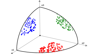
Figure 1: Illustration of normalized extremes $\theta_{i}$’s on the $\ell_{2}$-sphere of $\mathbb{R}_{+}^{3}$ with clusters of features $K_{1}=\{1,3\}$(blue), $K_{2}=\{1,2\}$(red) and $K_{3}=\{2,3\}$(green).

This paper provides a novel optimization-based approach for finding subspaces from multivariate extreme features. Given $n\geq 1$ i.i.d copies $X_{1},\ldots,X_{n}$ of a heavy-tailed random variable $X=(X^{1},\ldots,X^{p})\in\mathbb{R}^{p}$, the goal is to identify clusters of features $K\subset\llbracket 1,p\rrbracket$ such that the variables $\{X^{j}:j\in K\}$ may be large while the other variables $X^{j}$ for $j\notin K$ simultaneously remain small. Figure 1 depicts such an example of normalized extremes with the associated feature clusters.

Up to approximately $2^{p}$ combinations of extreme features are possible and contributions such as Chautru (2015); Chiapino & Sabourin (2016); Goix et al. (2016); Engelke & Hitz (2018); Chiapino et al. (2019) tend to identify a smaller number of simultaneous extreme features. Dimensional reduction methods such as principal components analysis and derivatives (Wold et al., 1987; Cutler & Breiman, 1994; Tipping & Bishop, 1999; Cooley & Thibaud, 2019; Drees & Sabourin, 2019) can be designed to find a lower dimensional subspace where extremes tend to concentrate. Following this path, the idea of the present paper is to decompose the $\ell_{1}$-norm of a positive input sample as a weighted sum of its features.

Several EVT contributions are aimed at assessing a sparse support of multivariate extremes (De Haan & Ferreira, 2007; Chiapino & Sabourin, 2016; Meyer & Wintenberger, 2019; Engelke & Ivanovs, 2020). A broader scope of contributions related to the work detailed in this paper ranges from compressed sensing (Candès et al., 2006; Candes et al., 2006; Tsaig & Donoho, 2006) and matrix factorization (Lee & Seung, 2001; Şimşekli et al., 2015) to group sparsity (Yuan & Lin, 2006; Simon et al., 2013; Devijver et al., 2015).

Contributions. The main results of this paper are:
(i) We present a novel optimization-based approach to perform subspace clustering of extreme regions in the multivariate framework. This is achieved by the algorithm Multivariate EXtreme Informative Clustering by Optimization (in short MEXICO) which finds a sparse representation for the dependence structure of extremes.
(ii) Following contribution laid out by Niculae et al. (2018), we study at length different manifolds on the probability simplex, including our $\mathbb{M}$-set. Our analysis may be of independent relevance.
(iii) The performance of the introduced algorithm are demonstrated from both theoretical and empirical points of view. First we provide a non-asymptotic bound on the excess risk. Secondly, numerical experiments on both feature clustering and anomaly detection tasks in extreme regions demonstrate the relevance of our method when compared to existing methods.

Notations. The following notations are used throughout the paper: $\mathcal{M}_{n}^{p}([1,+\infty[)$ is the set of $n\times p$ matrices valued in $[1,+\infty[$. Any matrix is denoted in bold. $\mathcal{A}_{p}^{m}$ denotes the set of mixture matrices composed of $p\times m$ matrices valued in $[0,1]$ where the sum of elements of any column equals $1$. For any $\mathbf{M}=(\mathbf{M}_{i}^{j})\in\mathcal{M}_{n}^{p}(\mathbb{R})$, for $i\in\llbracket 1,n\rrbracket$ (resp. $j\in\llbracket 1,p\rrbracket$), let $e_{i}$ (resp. $e^{j}$) denote the vector of the canonical basis such that $e_{i}\mathbf{M}=\mathbf{M}_{i}$ (resp. $\mathbf{M}e^{j}=\mathbf{M}^{j}$) where $M_{i}$ corresponds to the $i$-th line of $\mathbf{M}$ (resp. $M^{j}$ corresponds to the $j$-th column). Denote $\mathfrak{S}_{m}$ the finite symmetric group of order $m$. Let $E=[0,\infty]^{p}\backslash\{0\}$ and $\Omega_{p,||\cdot||}=\{x\in\mathbb{R}^{p}_{+}:\|x\|\leq 1\}$ the ball associated to the norm $||\cdot||$ and its complementary set $\Omega_{p,||\cdot||}^{c}=\mathbb{R}^{p}_{+}\backslash\Omega_{p}$, let $S$ denote the sphere associated to $\|\cdot\|$ and for $x\in\mathbb{R}^{p}$ and $K\subset\llbracket 1,p\rrbracket$, write $x^{(K)}=(x^{j}\mathds{1}_{j\in K})$. Denote by $\Gamma$ the Euler function.

Outline. The paper is organized as follows, in Section 2 we introduce the multivariate EVT background and our problem of interest. In Section 3 we present our optimization-based approach along with its specific details concerning the projection step onto the probability simplex. Section 4 gathers the theoretical results. We perform some numerical experiments in Section 5 to highlight the performance of our method and we finally conclude in Section 6. Proofs, technical details and additional results can be found in the appendix.

2 Preliminaries

Extreme value theory develops models for learning the unusual rather than the usual, in order to provide a reasonable assessment of the probability of occurrence of rare events. This section first recalls the required mathematical framework and classical tools for the analysis of multivariate extremes and then introduce our problem of interest.

2.1 Mathematical background

The notion of regular variation is a natural way for modelling power law behaviors that appear in various fields of probability theory. In this paper, we shall focus on the dependence and regular variation of random variables and random vectors. We refer to the book of Resnick (1987) for an excellent account of heavy-tailed distributions and the theory of regularly varying functions.

Definition 1

(Regular variation (Karamata, 1933)) A positive measurable function $g$ is regularly varying with index $\alpha\in\mathbb{R}$, notation $g\in\mathcal{R}_{\alpha}$ if $\lim_{x\to+\infty}g(tx)/g(x)=t^{\alpha}$ for all $t>0$.

The notion of regular variation is defined for a random variable $X$ when the function of interest is the distribution tail of $X$.

Definition 2

(Univariate regular variation) A non-negative random variable X is regularly varying with tail index $\alpha\geq 0$ if its right distribution tail $x\mapsto\mathbb{P}\left(X>x\right)$ is regularly varying with index $-\alpha$, i.e., $\lim_{x\to+\infty}\mathbb{P}\left(X>tx\;\middle|\;{}X>x\right)=t^{-\alpha}$ for all $t>1$.

This power-law behavior may be thought of as a smoothness condition for the tail at infinity. This definition can be extended to the multivariate setting where the topology of the probability space is involved. We rely on the vague convergence of measures (Resnick, 1987, Section 3.4) and consider the following definition (Resnick, 1986, p.69).

Definition 3

(Multivariate regular variation) A random vector $X\in\mathbb{R}_{+}^{p}$ is regularly varying with tail index $\alpha\geq 0$ if there exists $g\in\mathcal{R}_{-\alpha}$ and a nonzero Radon measure $\mu$ on $E$ such that

$$g(t)^{-1}\mathbb{P}\left(t^{-1}X\in A\right)\xrightarrow[t\to\infty]{}\mu(A),$$

where $A\subset E$ is any Borel set such that $0\not\in\partial A$ and $\mu(\partial A)=0$.

The limiting measure $\mu$, known as the exponent measure, is homogeneous of order $-\alpha$ i.e. for any $t>0$, $\mu(t\cdot)=t^{-\alpha}\mu(\cdot)$. This suggests a polar decomposition of $\mu$ into a radial component and an angular component $\Phi$. For any $x=(x_{1},\cdots,x_{p})\in\mathbb{R}^{p}_{+}$, one can set

$$\left\{\begin{array}[]{ll}R(x)&=||x||\\ \Theta(x)&=\left(\frac{x_{1}}{R(x)},\ldots,\frac{x_{p}}{R(x)}\right)\in S\end{array}\right.$$

For any $B\subset S$, the angular measure $\Phi$ on $S$ is defined as,

$$\Phi(B)\stackrel{{\scriptstyle\rm def}}{{=}}\mu(\{x,R(x)\geq 1,\Theta(x)\in B\}).$$

The angular measure $\Phi$ plays a central role in the analysis of extremes, as it characterizes the directions where extremes are more likely to occur. Assessing the support of $\Phi$, or equivalently of $\mu$, leads to forecasting the directions where extremes are more likely to occur i.e. features that are more likely to jointly be large.

2.2 Probabilistic Framework & Problem Statement

We observe $n\geq 1$ i.i.d copies $X_{1},\ldots,X_{n}$ of a regularly varying random vector $X=(X^{1},\ldots,X^{p})\in\mathbb{R}^{p}$ with tail index $\alpha=1$. Extremes correspond to samples with norm larger than a fixed threshold $t>0$. Incidentally, $t$ should depend on $n$, as the notion of extreme should be understood as large norms compared to the vast majority of observed data. The Euclidian space $\mathbb{R}^{p}$ being of finite dimension, all norms are equivalent and the choice of the norm does not matter for the definition of the limit measure (Beirlant et al., 2006), therefore we may use the $\ell_{\infty}$-norm in the remainder of this paper to analyse extremes. In other words $R(x)$ is set as $||.||_{\infty}$ in Definition 3. The observations are first sorted by decreasing order of magnitude $\|X_{(1)}\|_{\infty}\geq\ldots\geq\|X_{(n)}\|_{\infty}$. Then, consider a small fraction $0<\gamma<1$ of the observations and denote by $t_{\gamma}$ the quantile of $||X||_{\infty}$ at level $(1-\gamma)$, i.e. $\mathbb{P}\left(||X||_{\infty}>t_{\gamma}\right)=\gamma$. The extreme samples are $X_{(1)},\ldots,X_{(k)}$ where $k=\lfloor n\gamma\rfloor$ is a selection threshold (cf Remark 2).

Remark 1

(Pareto Standardization) In this work, it is assumed that all marginal distributions are tail equivalent to the Pareto distribution with index $\alpha=1$. In practice, the tails of the marginals may be different and it is convenient to work with marginally standardized variables. Thus, the margins $F^{j}(x^{j})=\mathbb{P}\left(X^{j}\leq x^{j}\right)$ are separated from the dependence structure in the description of the joint distribution of $X$. Consider the Pareto standardized variables $V^{j}=1/(1-F^{j}(X^{j}))\in[1,\infty]$ and $V=T(X)=(V^{1},\ldots,V^{d})$. Replacing X by V permits to take $\alpha=1$ and $g(t)=1/t$ in Definition 3. Appendix B.1 provides further details concerning $\widehat{T}$ the empirical counterpart of $T$.

Remark 2

(On selection of $k$) Determining $k$ is a central bias variance trade-off of Extreme Value analysis (See e.g. Goix et al. (2016) and references therein). As $k$ gets too large, a bias is induced by taking into account observations which do not necessarily behave as extremes: their distribution deviates significantly from the limit distribution of extremes. On the other hand, too small values lead to an increase of the algorithm’s variance.

Our work focuses on assessing the dependence structure in extreme regions in a multivariate setup. The angular measure $\Phi$ fully describes the latter asymptotic dependence. Therefore, we seek to accurately infer a sparse summary of the mass of extremes spread on each constructed subspace.
Let $X\in\mathbb{R}_{+}^{p}$ be a multivariate random vector whose dependence structure is unknown. We address the problem of finding different feature clusters $K_{j}\subset\llbracket 1,p\rrbracket$ with $j=1,\ldots,m$ and $m<p$ such that all features in a same subset may be large together. In order to reach a representation of interest, e.g., diversity for portfolio in finance or clusters for smart grids in wireless technologies, we seek disjoint clusters ($K_{i}\cap K_{j}=\emptyset$ for all $i\neq j$). Relying on the $m$ clusters of features $K_{1},\ldots,K_{m}$ and the underlying subspaces, the exponent measure $\mu$ can be approximated as $\mu(\cdot)\approx\sum_{j=1}^{m}\mu_{K_{j}}(\cdot)$. Each component $\mu_{K_{j}}$ is concentrated on the subregion given by the features of cluster $K_{j}$.

In the remaining of this paper, $\mathbf{X}\in\mathcal{M}_{k,p}([1,+\infty[)$ corresponds to the truncated training set: $X_{(1)},\ldots,X_{(k)}$. We search a subset $K$ of features such that the $\ell_{1}$-norms of $\mathbf{X}_{i}$ and its restriction $\widetilde{\mathbf{X}}_{i}=\mathbf{X}_{i}^{(K)}$ are almost equal i.e.

$$\|\widetilde{\mathbf{X}}_{i}\|_{1}\approx\|\mathbf{X}_{i}\|_{1}.$$

3 Feature Mixture in Extreme Regions

This section presents an approach to find relevant directions of the extreme samples to estimate the support of $\mu$. The analysis is carried out under the empirical risk minimization paradigm and details our algorithm MEXICO.

3.1 Empirical Risk Minimization

To assess the dependence structure of features of extreme samples, we consider the framework of empirical risk minimization focused on extreme regions. Consider an extreme sample $X$, i.e., an observation satisfying $\|X\|_{\infty}>t_{\gamma}$. The goal is to learn a representation function $g:\mathbb{R}^{p}\to\mathbb{R}_{+}$ in order to minimize the Bayes risk at level $t_{\gamma}$ defined by

$$\mathcal{R}_{t_{\gamma}}(g)={{\mathbb{E}}}_{X}\left[\ell\left(X,g\left(X\right)\right)\Big{|}\|X\|_{\infty}>t_{\gamma}\right],$$ (1)

where $\ell:\mathbb{R}_{+}^{p}\times\mathbb{R}_{+}\to\mathbb{R}_{+}$ is a loss function measuring the discrepancy between the true extreme dependence structure of $X$ and its predicted counterpart $g\left(X\right)$. Based on the extreme observations $X_{(1)},\ldots,X_{(k)}$, the empirical risk in the extreme regions is given by

$$\widehat{\mathcal{R}}_{k}(g)=\frac{1}{k}\sum_{i=1}^{k}\ell\big{(}X_{(i)},g(X_{(i)})\big{)}.$$ (2)

Features mixtures. In order to recover the clusters of features, we consider mixtures of the components of each sample. The true number of subregions is unknown and we search for $m$ clusters where $m$ is selected according to Remark 3. We consider the probability simplex $\Delta_{p}$ defined on the positive orthant of $\mathbb{R}_{+}^{p}$ by

$$\Delta_{p}=\{x\in\mathbb{R}^{p}_{+},x_{1}+\ldots+x_{p}=1\},$$

and let $\mathbf{W}\in\mathcal{A}_{p}^{m}$ with $m<p$ be a mixture matrix. We denote by $\widetilde{\mathbf{X}}=\mathbf{X}\mathbf{W}\in\mathcal{M}_{k}^{m}(\mathbb{R}_{+})$ the transformed matrix. The following proposition ensures the preservation of the regular variation of the resulting vectors $\widetilde{X}_{i}$’s.

Proposition 1 (Mixture transformation)

Let $X\in\mathbb{R}_{+}^{p}$ be a regularly varying vector as defined earlier and $\mathbf{W}\in\mathcal{A}_{p}^{m}$ a mixture matrix with $1<m\leq p$. Then the transformed vector $\widetilde{X}=X\mathbf{W}\in\mathbb{R}_{+}^{m}$ is regularly varying with tail index $\alpha=1$. Thereby, if we denote by $\mu$ (resp. $\widetilde{\mu}$) the limiting measure of $X$ (resp. $\widetilde{X}$), we have

$$(1/m)\widetilde{\mu}(\Omega_{m,||\cdot||_{1}}^{c})\leq\widetilde{\mu}(\Omega_{m,||\cdot||_{\infty}}^{c})\leq\mu(\Omega_{p,||.||_{1}}^{c}).$$

The proof of the proposition is deferred to the appendix.

Remark 3

(Selection of $m$) In view of Proposition 1, in practice, the required dimension $m<p$ can be seen as the smallest value $m$ such that the empirical version of $\widetilde{\mu}(\Omega_{m,||.||_{\infty}}^{c})$ is arbitrarly close to the empirical version of $\mu(\Omega_{p,||.||_{1}}^{c})$. Hence, the $m$ selected clusters provide relevant support of extremes.

Loss function. A natural question rises in the choice of the approximation function $g$ used in Eq. (1). Each column $\mathbf{W}^{j}$ for $j\in\llbracket 1,m\rrbracket$ is modelling a mixture of components and represents a cluster $K_{j}$. For any sample $X$, we want to find a mixture that gives a good approximation in $\ell_{1}$-norm, i.e., we seek a column $j\in\llbracket 1,m\rrbracket$ for which $\widetilde{{X}}^{j}=(X\mathbf{W})^{j}$ is the closest to $\|X\|_{1}$. A simple choice for the approximation function $g$ is reached through a linear combination and defined as follows for any input $x\in\mathbb{R}^{p}_{+}$,

$$g_{\mathbf{W}}:x\mapsto g_{\mathbf{W}}(x)=\max_{1\leq j\leq m}(x\mathbf{W})^{j}.$$ (3)

The associated loss function is defined by

$$\ell\left(x,g_{\mathbf{W}}(x)\right)=\frac{1}{p}\left(\|x\|_{1}-g_{\mathbf{W}}(x)\right).$$ (4)

Observe that this particular choice yields a loss function bounded in $[0,1]$ when using the angular decomposition of extremes $\theta=X/\|X\|_{\infty}$. With this choice, the approximation function $g_{\mathbf{W}}$ is parametrized by the mixture matrix $\mathbf{W}$. For ease of notation we abusively denote by $\ell(X,\mathbf{W})=\ell(X,g_{\mathbf{W}}(X))$. Thus, using this specific loss in Eq. (1), the goal is to learn the mixture matrix $\mathbf{W}_{t}^{\star}$ minimizing the risk on extremes

$$\mathbf{W}_{t}^{\star}\in\mathop{\rm arg\,min}_{\mathbf{W}\in\mathcal{A}_{p}^{m}}\left\{\mathcal{R}_{t}(\mathbf{W})\stackrel{{\scriptstyle\rm def}}{{=}}{{\mathbb{E}}}\left[\ell\left(X,\mathbf{W}\right)|\|X\|_{\infty}>t\right]\right\}.$$

Based on the observations $\{X_{(1)},\ldots,X_{(k)}\}$, the optimization problem consists in finding a mixture matrix minimizing the empirical risk

$$\widehat{\mathbf{W}}_{k}\in\mathop{\rm arg\,min}_{\mathbf{W}\in\mathcal{A}_{p}^{m}}\left\{\widehat{\mathcal{R}}_{k}(\mathbf{W})=\frac{1}{k}\sum_{i=1}^{k}\ell\left(X_{(i)},\mathbf{W}\right)\right\}$$ (5)

Note that $\mathcal{A}_{p}^{m}$ is a closed and bounded set hence compact (Bourbaki, 2007) thus there exists at least one solution which can be reached. The minimization problem of Eq. (5) can be rewritten as

$$\widehat{\mathbf{W}}_{k}\in\mathop{\rm arg\,max}_{\mathbf{W}\in\mathcal{A}_{p}^{m}}\frac{1}{k}\sum_{i=1}^{k}g_{\mathbf{W}}(X_{(i)}).$$

The index of the column representing a good mixture can be defined with the mapping

$$\varphi:\llbracket 1,k\rrbracket\to\llbracket 1,m\rrbracket,\quad\varphi(i)=\mathop{\rm arg\,max}_{1\leq j\leq m}\widetilde{X}_{(i)}^{j}$$

and the optimization problem becomes

$$\mathop{\rm arg\,max}_{\mathbf{W}\in\mathcal{A}_{p}^{m}}\left\{\frac{1}{k}\sum_{i=1}^{k}(\mathbf{X}\mathbf{W})_{i}^{\varphi(i)}=\frac{1}{k}\sum_{i=1}^{k}e_{i}(\mathbf{X}\mathbf{W})e^{\varphi(i)}\right\}.$$ (6)

Illustrative example. As a first go, consider the following example showing the way the matrix $\mathbf{W}$ recovers the different clusters. Assume that the vector $X\in\mathbb{R}_{+}^{p}$ is exactly coming from a mixture of $m$ disjoint clusters $K_{1},\ldots,K_{m}$ and for each sample $\mathbf{X}_{i}$, there exists $K_{j}$ such that $\|\mathbf{X}_{i}^{(K_{j})}\|_{1}=\|\mathbf{X}_{i}\|_{1}$. For all $j\in\llbracket 1,m\rrbracket$, denote $U^{j}\in[0,1]^{p}$ the uniform vector with support $K_{j}$, i.e., $U^{j}=(1/|K_{j}|)^{(K_{j})}$. A solution to the optimization problem is given by any column-permutation of the matrix ${\mathbf{W}}$ whose columns are the vectors $U^{j}$. Indeed, the transformed data matrix is $\widetilde{\mathbf{X}}=\mathbf{X}\mathbf{W}$ and for any sample $\mathbf{X}_{i}$ whose features are coming from a cluster $K_{j}$, we have

$$\forall l\neq j,\quad\widetilde{\mathbf{X}}_{i}^{j}=\mathbf{X}_{i}U^{j}=\mathbf{X}_{i}^{(K_{j})}U^{j}\geq\mathbf{X}_{i}U^{l}=\widetilde{\mathbf{X}}_{i}^{l}.$$

Taking $\varphi(i)=\mathop{\rm arg\,max}_{1\leq l\leq m}\widetilde{\mathbf{X}}_{i}^{l}$ exactly recovers the cluster of index $j=\varphi(i)$. In the case where the large features of the different sample $\mathbf{X}_{i}$ are all equal, then the columns of the mixture matrix $\mathbf{W}$ tend exactly to uniform vectors with restricted support.

3.2 Optimization on the Simplex

Problem relaxation. One can directly solve the linear program (6) but this formulation suffers from drawbacks. First, the solution could belong to a vertex of the simplex and would induce a unique direction. Second, it involves finding the mapping $\varphi$ among all the possible combinations which can be prohibited when $k$ or $p$ increases. Thus, one can solve a relaxed version of Eq. (6) by introducing another matrix of mixtures $\mathbf{Z}\in\mathcal{A}_{m}^{k}$. The relaxed problem is

$$(\widehat{\mathbf{W}}_{k},\widehat{\mathbf{Z}}_{k}) \in\mathop{\rm arg\,max}_{(\mathbf{W},\mathbf{Z})\in\mathcal{A}_{p}^{m}\times\mathcal{A}_{m}^{k}}\frac{1}{k}\sum_{i=1}^{k}\mathbf{X}_{i}\mathbf{W}\mathbf{Z}^{i}.$$ (7)

Optimization problem. We recognize the trace operator in Eq. (7) which is linear and can define an objective function $f:\mathcal{A}_{p}^{m}\times\mathcal{A}_{m}^{k}\to\mathbb{R}$ that we need to maximize:

$$\left\{\begin{array}[]{ll}(\widehat{\mathbf{W}}_{k},\widehat{\mathbf{Z}}_{k})\in\mathop{\rm arg\,max}_{(\mathbf{W},\mathbf{Z})}f(\mathbf{W},\mathbf{Z})\\ f(\mathbf{W},\mathbf{Z})=Tr(\mathbf{XWZ})/k\end{array}\right.$$

The objective function $f$ is bilinear in finite dimension hence continuous. Since maximization occurs on compact sets, there is at least one solution $(\widehat{\mathbf{W}}_{k},\widehat{\mathbf{Z}}_{k})$. However, it is not unique since any column-permutation of $\widehat{\mathbf{W}}_{k}$ along with the associated row-permutation of $\widehat{\mathbf{Z}}_{k}$ is also a valid solution. Indeed, any column (resp. row) permutation consists of a multiplication on the right (resp. left) side by a permutation matrix. For any $\sigma\in\mathfrak{S}_{k}$, consider the permutation matrix $\mathbf{P}_{\sigma}=(\delta_{i,\sigma(j)})_{1\leq i,j\leq m}$. We have $\mathbf{P}_{\sigma}^{T}=\mathbf{P}_{\sigma^{-1}}$ so that

$$(\widehat{\mathbf{W}}_{k}\mathbf{P}_{\sigma})(\mathbf{P}_{\sigma}^{T}\widehat{\mathbf{Z}}_{k})=\widehat{\mathbf{W}}_{k}(\mathbf{P}_{\sigma}\mathbf{P}_{\sigma^{-1}})\widehat{\mathbf{Z}}_{k}=\widehat{\mathbf{W}}_{k}\widehat{\mathbf{Z}}_{k}.$$

One may refer to (Meilă, 2006, 2007) for a discussion on the permutations of clustering solutions.

Regularization. The constraint of disjoint clusters can be satisfied by forcing the columns of the mixture matrix $\mathbf{W}$ to be orthogonal, i.e., for all $i<j,\langle W^{i},W^{j}\rangle=0$. This yields a penalized version of the objective function with a regularization parameter $\lambda>0$

$$\left\{\begin{array}[]{ll}(\widehat{\mathbf{W}}_{k},\widehat{\mathbf{Z}}_{k})\in\mathop{\rm arg\,max}_{(\mathbf{W},\mathbf{Z})}f_{\lambda}(\mathbf{W},\mathbf{Z})\\ f_{\lambda}(\mathbf{W},\mathbf{Z})=Tr(\mathbf{X}\mathbf{W}\mathbf{Z})/k-\lambda\sum_{i<j}\langle W^{i},W^{j}\rangle\end{array}\right.$$

with partial derivatives given by

$$\left\{\begin{array}[]{ll}\nabla_{\mathbf{Z}}f_{\lambda}(\mathbf{W},\mathbf{Z})&=(\mathbf{X}\mathbf{W})^{T}/k\\ \nabla_{\mathbf{W}}f_{\lambda}(\mathbf{W},\mathbf{Z})&=(\mathbf{Z}\mathbf{X})^{T}/k-\lambda\widetilde{\mathbf{W}},\widetilde{W}^{j}=\sum_{i<j}W^{i}.\end{array}\right.$$

Update rule. The optimization problem can be addressed using an alternate scheme by computing projected gradient ascent at each iteration

$$\left\{\begin{array}[]{ll}\mathbf{W}_{k+1}&=\Pi_{\mathcal{S}}\left(\mathbf{W}_{k}+\delta_{k}^{W}\nabla_{\mathbf{W}}f_{\lambda}(\mathbf{W}_{k},\mathbf{Z}_{k})\right)\\ \mathbf{Z}_{k+1}&=\Pi_{\Delta_{m}}\left(\mathbf{Z}_{k}+\delta_{k}^{Z}\nabla_{\mathbf{Z}}f_{\lambda}(\mathbf{W}_{k+1},\mathbf{Z}_{k})\right)\end{array}\right.$$ (8)

where $\Pi_{\mathcal{S}}(\cdot),\Pi_{\triangle_{m}}(\cdot)$ are respectivetly the projection of each column onto a convex set $\mathcal{S}\subset\Delta_{p}$ and onto the probability simplex $\Delta_{m}$. The learning rates $\delta_{k}^{W},\delta_{k}^{Z}$ are step sizes found by backtracking line search. The convergence property of the optimization procedure is the same as the convergence of projected gradient descent as detailed in Calamai & Moré (1987); Dunn (1987).

Figure 2: Simplex of $\mathbb{R}^{3}$ with $\mathcal{S}_{3}^{\ell_{1}}$ (left), $\mathcal{S}_{3}^{\ell_{2}}$(center) and the $\mathbb{M}$-set $\mathcal{S}_{3}^{\tau}$(right).

Projection step on $\mathcal{S}$. In order to recover clusters that are not unit sets, we want to avoid the vertices of the simplex. Thus, we perform a projection step $\Pi_{\mathcal{S}}(\cdot)$ of each column of $\mathbf{W}$ onto a convex set $\mathcal{S}$. Several choices are to be considered, as illustrated in Figure 2. Denote $\bar{x}=(1/p,\ldots,1/p)$ the barycenter of the probability simplex $\Delta_{p}$ and consider the following manifolds:
(i) $\ell_{1}$ incircle: the coordinate permutations of $(0,1/(p-1),\ldots,1/(p-1))$ are the centers of the faces of $\Delta_{p}$ and they define a reversed and scaled simplex $\mathcal{S}_{p}^{\ell_{1}}$.
(ii) $\ell_{2}$ incircle: consider the euclidian ball $B_{2,p}(\bar{x},r)=\{x\in\mathbb{R}^{p}|\|x-\bar{x}\|_{2}\leq r\}$. The radius value $r_{p}=1/\sqrt{p(p-1)}$ yields the $\ell_{2}$ inscribed ball of $\Delta_{p}$ along with $\mathcal{S}_{p}^{\ell_{2}}=\Delta_{p}\cap B_{2,p}(\bar{x},r_{p})$.
(iii) $\mathbb{M}$-set: The previous manifolds do not scale well as the dimension grows and we shall discuss some theoretical results to see that their hypervolumes become very small. To escape from the curse of dimensionality, we consider the convex set where we cut off the vertices using a threshold $\tau$ of the distance $L=\|\bar{x}-e_{j}\|_{2}=\sqrt{(p-1)/p}$ between the barycenter and a vertex. It is also the intersection of the simplex $\Delta_{p}$ and an $\ell_{\infty}$ ball. We call this manifold the $\mathbb{M}$-set $\mathcal{S}_{p}^{\tau}$ defined as

$$\mathcal{S}_{p}^{\tau}=\left\{x\in\Delta_{p}|\max_{1\leq j\leq p}\left\langle x-\bar{x},e_{j}-\bar{x}\right\rangle\leq\tau\|e_{j}-\bar{x}\|_{2}\right\}.$$

Define the radius $r_{\infty}^{p}(\tau)=1-(1-\tau)(p-1)/p$ then the $\mathbb{M}$-set may be seen as the intersection of the simplex with a particular $\ell_{\infty}$ ball as

$$\mathcal{S}_{p}^{\tau}=\Delta_{p}\cap B_{\infty,p}\left(\bar{x},\tau L\right)=\Delta_{p}\cap B_{\infty,p}\left(0,r_{\infty}^{p}(\tau)\right).$$

The projection onto the simplex is a well-studied subject (Daubechies et al., 2008; Duchi et al., 2008; Chen & Ye, 2011; Condat, 2016). For the projection onto the intersection of convex sets, one can perform a naive approach of alternate projections (Gubin et al., 1967) or some refinements using the idea of Dykstra’s algorithm (Dykstra, 1983; Boyle & Dykstra, 1986; Bregman et al., 2003).

3.3 MEXICO Algorithm

Starting from random matrices $(\mathbf{W}_{0},\mathbf{Z}_{0})\in\mathcal{A}_{p}^{m}\times\mathcal{A}_{m}^{k}$, the update rule of Eq. (8) returns a pair of matrices $(\mathbf{W}_{mex},\mathbf{Z}_{mex})$ that are of great interest to analyze the dependence structure of the most extreme data and thus the support of extremes. On the one hand, the mixture matrix $\mathbf{W}_{mex}$ gives insights about the different clusters of features that are large simultaneously. On the other hand, the matrix $\mathbf{Z}_{mex}$ gives information about the probability of belonging to each cluster. Each column $\mathbf{W}_{mex}^{j}$ represents a cluster $K_{j}$ and for each sample $\mathbf{X}_{i},i\in\llbracket 1,k\rrbracket$, the $j^{th}$-row of the column $\mathbf{Z}_{mex}^{i}$ is the confidence for $X_{i}$ to belong to the cluster $K_{j}$.

A detailed pseudo-code of MEXICO is provided below in Algorithm 1. Since the margins of the data may be unknown, one could work with $\widehat{T}$ which is the empirical counterpart of the Pareto standardization $T$ as detailed in Appendix B.1. The output of the algorithm may be used for feature clustering (FC) or anomaly detection (AD) tasks.

Algorithm 1 MEXICO algorithm

0:  Training data $(X_{1},\ldots,X_{n}),0<m<p,\lambda>0$ and rank $k(=\lfloor n\gamma\rfloor)$.

1:  Initialize $(\mathbf{W}_{0},\mathbf{Z}_{0})\in\mathcal{A}_{p}^{m}\times\mathcal{A}_{m}^{n}$.

2:  Standardize the data $\widehat{V}_{(i)}=\widehat{T}(X_{(i)})$ (see Remark 1).

3:  Sort training data by decreasing order of magnitude         $\|\widehat{V}_{(1)}\|_{\infty}\geq\ldots\geq\|\widehat{V}_{(n)}\|_{\infty}$.

4:  Consider the set of $k$ extreme training data $\widehat{V}_{(1)},\ldots,\widehat{V}_{(k)}$.

5:  Compute $(\mathbf{W}_{mex},\mathbf{Z}_{mex})\in\mathop{\rm arg\,max}_{(\mathbf{W},\mathbf{Z})}f_{\lambda}(\mathbf{W},\mathbf{Z})$ using update rule (8).

6:  Given a new input ${X}_{\text{new}}$ standardized as $\widehat{V}_{\text{new}}$ with $\|\widehat{V}_{\text{new}}\|_{\infty}\geq\|\widehat{V}_{(k)}\|_{\infty}$, compute $\widetilde{V}_{\text{new}}=\widehat{V}_{\text{new}}\mathbf{W}_{mex}$.

7:  Compute predicted cluster $\varphi_{0}=\mathop{\rm arg\,max}_{1\leq j\leq m}{\widetilde{V}_{\text{new}}^{j}}$.

8:  (FC) Return cluster $\varphi_{0}$. (AD) Return score $\ell(\widetilde{V}_{\text{new}},\mathbf{W}_{{mex}})$.

4 Theoretical Study

This section provides some theoretical results. First, a theoretical analysis of the $\mathbb{M}$-set is established. In order to compare the different manifolds of the previous section, we analyze the volume reduction performed in each case. Second, a non-asymptotic bound for the excess risk is detailed.

Theorem 1 (Volume and ratio)

Consider the probability simplex $\Delta_{p}$ and the different manifolds $\mathcal{S}_{p}^{\ell_{1}},\mathcal{S}_{p}^{\ell_{2}},\mathcal{S}_{p}^{\tau}$. For any bounded set $\mathcal{D}\subset\mathbb{R}^{p}$, define its hypervolume $\mathcal{V}ol(\mathcal{D})$ and its ratio $\rho(\mathcal{D})$ as

$$\mathcal{V}ol(\mathcal{D})=\int_{\mathbb{R}^{p}}\mathds{1}_{\mathcal{D}}(x)\mathrm{d}x,\quad\rho(\mathcal{D})=\mathcal{V}ol(\mathcal{D})/\mathcal{V}ol(\Delta_{p}).$$

$\mathcal{S}$	Hypervolume $\mathcal{V}ol(\mathcal{S})$
$\Delta_{p}$	$\frac{\sqrt{p}}{\Gamma(p)}$
$\mathcal{S}_{p}^{\ell_{1}}$	$\frac{\sqrt{p}}{\Gamma(p)}\left(\frac{1}{(p-1)^{(p-1)}}\right)$
$\mathcal{S}_{p}^{\ell_{2}}$	$\frac{\sqrt{p}}{\Gamma(p)}\left(\frac{\Gamma(p)}{\Gamma\left(\frac{p+1}{2}\right)}\frac{\pi^{(p-1)/2}}{\sqrt{p^{p}(p-1)^{(p-1)}}}\right)$
$\mathcal{S}_{p}^{\tau}$	$\frac{\sqrt{p}}{\Gamma(p)}\left(1-p(1-\tau)^{(p-1)}\left(\frac{p-1}{p}\right)^{(p-1)}\right)$

The corresponding ratios are given by

$$\left\{\begin{array}[]{ll}\rho(\mathcal{S}_{p}^{\ell_{1}})&=\frac{1}{(p-1)^{(p-1)}}\\ \rho(\mathcal{S}_{p}^{\ell_{2}})&=\frac{\Gamma(p)}{\Gamma\left(\frac{p+1}{2}\right)}\frac{\pi^{(p-1)/2}}{\sqrt{p^{p}(p-1)^{(p-1)}}}\\ \rho(\mathcal{S}_{p}^{\tau})&=1-p\left[(1-\tau)\left(\frac{p-1}{p}\right)\right]^{(p-1)}\end{array}\right.$$

Moreover, when the dimension grows $p\to+\infty$ and for a fixed $\tau\in(0,1)$, we have $\rho(\mathcal{S}_{p}^{\ell_{1}})\to 0$, $\rho(\mathcal{S}_{p}^{\ell_{2}})\to 0$ and $\rho(\mathcal{S}_{p}^{\tau})\to 1.$ Among studied subsets, in a high-dimensional setting the $\mathbb{M}$-set is the only one not collapsing towards a unit set.

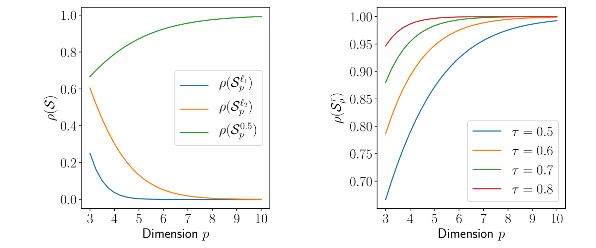
Figure 3: Evolution of the Ratio Volume with dimension $p$.

Remark 4

(Selection of $\tau$) With a high reduction of the probability simplex (i.e. $\tau\to 0$), the vertices are avoided but discriminating the clusters is harder as the $\mathbb{M}$-set tends to the barycenter of the simplex. This trade-off motivates the choice of the threshold $\tau$ and Figure 3 shows the evolution of the ratios $\rho$ for the different manifolds.

The following proposition, whose proof is deferred to the appendix, shows that MEXICO algorithm can be seen as a contraction mapping.

Proposition 2 (Lipschitz mapping)

Given $x_{1},x_{2}\in\mathbb{R}^{p}_{+}$ with norms greater than $t>0$ the application $x\mapsto x\mathbf{W}_{t}^{\star}$ is $\frac{m}{2}$-lipschitz continuous i.e.,

$$||x_{1}\mathbf{W}_{t}^{\star}-x_{2}\mathbf{W}_{t}^{\star}||_{2}\leq\frac{m}{2}||x_{1}-x_{2}||_{2}.$$

Moreover, if $x_{1}$ and $x_{2}$ belong to the same feature cluster $K$ then $||x_{1}\mathbf{W}_{t}^{\star}-x_{2}\mathbf{W}_{t}^{\star}||_{2}\leq\frac{1}{2}||x_{1}-x_{2}||_{2}.$ Hence, the transformation induced by MEXICO can be considered as a cluster contraction mapping (Boyd & Wong, 1969).

Finally, the convergence rate of our method can be analyzed through the non-asymptotic bound on the risks (1) and (2). The following Theorem provides an upper bound for the excess risk. The proof is given in the appendix.

Theorem 2 (Non-asymptotic bound)

Consider the risk $\mathcal{R}_{t_{\gamma}}$ defined in (1) associated to the loss function (4) computed on normalized data. Recall that $k=\lfloor n\gamma\rfloor$ and denote by $\mathbf{W}_{mex}$ the mixture matrix obtained by MEXICO. Then for $\delta\in(0,1)$, $n\geq 1$ and $\tau\leq 1$ we have with probability at least $1-\delta$,

$$\mathcal{R}_{t_{\gamma}}(\mathbf{W}_{mex})-\mathcal{R}_{t_{\gamma}}(\mathbf{W}_{t_{\gamma}}^{\star})\leq\frac{1}{\sqrt{k}}8\sqrt{2(1-\gamma)\log(4/\delta)}\ +$$

$$\frac{1}{k}\bigg{(}\frac{16}{3}\log(4/\delta)+8\sqrt{2(1-\gamma)\log(4/\delta)}+2\bigg{)}+2r_{\infty}^{p}(\tau).$$

The upper bound stated above shows that the convergence rate is of order $O_{\mathbb{P}}(1/\sqrt{k})$ where $k$ is the actual size of the dataset required to estimate the support of extreme. This convergence rate matches the one of Goix et al. (2016).

5 Numerical Experiments

We focus on popular machine learning tasks of feature clustering and anomaly detection to compare the performance of our algorithm against state-of-the-art methods for extreme events. Since the margins distributions of real-world data are unknown, the rank transformation as described in Remark 1 is considered. For ease of reproducibility, the code is available upon request.

5.1 Feature Clustering

Consider the feature clustering task where a new extreme sample $X_{\text{new}}\in\mathbb{R}_{+}^{p}$ is to be analyzed. Since $X_{\text{new}}$ is extreme, our goal is to predict the features that are large simultaneously based on the dependence structure clusters, i.e. the clusters given by MEXICO. For that matter, one can compute the transformed sample $\widetilde{X}_{\text{new}}=X_{\text{new}}\mathbf{W}_{mex}$ and assign the predicted cluster of features by $\text{Pred}(X_{\text{new}})=\mathop{\rm arg\,max}_{1\leq j\leq m}{\widetilde{X}_{\text{new}}^{j}}$.

Since MEXICO is an inductive clustering method, we focus on similar clustering algorithms namely spectral clustering (Ding et al., 2005) and spherical K-means (Janßen et al., 2020). Janßen et al. (2020) studied spherical K-means algorithm as a solution to perform clustering in extremes. We consider simulated data from an (asymmetric) logistic distribution where the dependence structure of extremes can be specified (see Appendix B.2). Given the ground truth class samples, we leverage metrics using conditional entropy analysis: Rosenberg & Hirschberg (2007) define the following desirable objectives for any cluster assignment: Homogeneity (H), each cluster contains only members of a single class; Completeness (C), all members of a given class are assigned to the same cluster; v-Measure (v-M): the harmonic mean of Homogeneity and Completeness.

The parameter setting is the following: dimension $p\in\{75,100,150,200\}$, number of train samples $n_{\text{train}}=1000$ and test samples $n_{\text{test}}=100$. We use the metrics implemented by Scikit-Learn (Pedregosa et al., 2011). The results, obtained over $100$ independently simulated dataset for each value of $p$, are gathered in Table 1, where the values associated to MEXICO transcribe the best performance between projection method with Dykstra’s algorithm and alternating projection. Both methods are detailed in the appendix. For each dimension $p$, bold characters indicate the best method when results are statistically significant using Mann-Whitney and Neyman-Pearson tests.

$p$	Spectral Clustering (Ding et al., 2005)
	H	C	v-M
75	0.925$\pm$ 0.054	0.937$\pm$0.040	0.931 $\pm$0.046
100	0.918$\pm$0.058	0.934$\pm$0.039	0.926$\pm$0.048
150	0.889$\pm$ 0.060	0.925$\pm$0.031	0.906$\pm$ 0.045
200	0.886$\pm$0.047	0.928$\pm$0.024	0.906$\pm$0.034
$p$	Spherical-Kmeans (Janßen et al., 2020)
	H	C	v-M
75	0.950$\pm$0.034	0.972$\pm$0.024	0.961$\pm$0.027
100	0.943$\pm$0.031	0.967$\pm$0.024	0.955$\pm$0.026
150	0.940$\pm$ 0.026	0.962$\pm$0.020	0.951$\pm$0.022
200	0.940$\pm$0.018	0.962$\pm$0.014	0.951$\pm$0.015
$p$	MEXICO
	H	C	v-M
75	0.978$\pm$0.025	0.976$\pm$0.024	0.977$\pm$0.024
100	0.978$\pm$0.020	0.979$\pm$0.021	0.978$\pm$0.020
150	0.976$\pm$0.015	0.980$\pm$0.013	0.978$\pm$0.014
200	0.970$\pm$0.015	0.975$\pm$0.012	0.972$\pm$0.013

Table 1: Comparison of Homogeneity (H), Completeness (C) and v-Measure (v-M) on Simulated Data.

5.2 Anomaly Detection

To predict whether a new extreme sample $X_{\text{new}}\in\mathbb{R}_{+}^{p}$ is an anomaly, one may use the value of the loss function $\ell(X_{\text{new}},\mathbf{W}_{\text{mex}})$ as an anomaly score. If it is small then the dependence structure of $X_{\text{new}}$ is well captured by the mixture $\mathbf{W}_{{mex}}$ and the behavior is rather normal. Conversely, a high value means that $X_{\text{new}}$ cannot be approximated by a mixture of $\mathbf{W}_{mex}$ i.e. it is more likely to be an outlier. The behavior of the extreme sample $X_{\text{new}}$ can be predicted using any decreasing function of the loss function $\ell$. In the experiment we use the inverse of the loss though one could consider the opposite of the loss as in (Goix et al., 2016).

We perform a comparison of three algorithms for anomaly detection in extreme regions: Isolation Forest (Liu et al., 2008), DAMEX (Goix et al., 2017) and our method MEXICO. The algorithms are trained and tested on the same datasets, the test set being restricted to extreme regions. Five reference AD datasets are studied: shuttle, forestcover, http, SF and SA. Table 5 in the Appendix provides further dataset details. The experiments are performed in a semi-supervised framework where the training set consists of normal data only. More details about the preprocessing, model tuning and additional results are available in the appendix. The results of means and standard deviations are obtained over $100$ runs and summarized in Table 2. Better performance are obtained with our anomaly detection approach compared to competing anomaly detection methods.

Dataset	ROC-AUC	AP
	iForest (Liu et al., 2008)
SA	0.886$\pm$0.032	0.879$\pm$0.031
SF	0.381$\pm$0.086	0.393$\pm$0.081
http	0.656$\pm$0.094	0.658$\pm$0.099
shuttle	0.970$\pm$0.020	0.826$\pm$0.055
forestcover	0.654$\pm$0.096	0.894$\pm$0.037
	DAMEX (Goix et al., 2016)
SA	0.982$\pm$0.002	0.938$\pm$0.012
SF	0.710$\pm$0.031	0.650$\pm$0.034
http	0.996$\pm$0.002	0.968$\pm$0.009
shuttle	0.990$\pm$0.003	0.864$\pm$0.026
forestcover	0.762$\pm$0.008	0.893$\pm$0.010
	MEXICO
SA	0.983$\pm$0.031	0.950$\pm$0.011
SF	0.892$\pm$0.013	0.812$\pm$0.016
http	0.997$\pm$0.002	0.972$\pm$0.012
shuttle	0.990$\pm$0.003	0.864$\pm$0.037
forestcover	0.863$\pm$0.015	0.958$\pm$0.006

Table 2: Comparison of Area Under Curve of Receiver Operating Characteristic (ROC-AUC) and Average Precision (AP).

6 Conclusion

Understanding the impact of shocks, i.e., extremely large input values on systems is of critical importance in diverse fields ranging from security or finance to environmental sciences and epidemiology. In this paper, we have developed a a rigorous methodological framework for clustering features in extreme regions, relying on the non-parametric theory of regularly varying random vectors. We illustrated our algorithm performance for both feature clustering and anomaly detection on simulated and real data. Our approach does not scan all the multiple possible subsets and outperforms existing algorithms. Future work will focus on the statistical properties of the developed algorithm by further exploring links with kernel methods.

Section A gathers the proofs of theorems and propositions. Section B details the probabilistic framework of EVT through Pareto standardization and logistic distributions. Section C highlights links with self-supervised methods related to MEXICO. Section D is dedicated to numerical experiments: the preprocessing of the data, models selection and additional results. Further numerical experiments and variants are gathered in Section E.

Appendix A Proofs of Theorems & Propositions

A.1 Proof of Proposition 1

proof.  Proposition 1 can be derived from Engelke et al. (2018)[Theorem 2] and we provide another proof for the sake of clarity. $X$ is a standard regularly varing where with margin tails equivalent to Pareto distribution. Using the characterization of Basrak et al. (2002), we have the following equivalence between the behavior of the vector and its components

$$\left(X\text{ is regularly varying}\right)\iff\left(\forall u\in\mathbb{R}^{p},\langle u,X\rangle\text{ is univariate regularly varying}\right)$$

Each column $\widetilde{X}^{j}$ of $\widetilde{X}=XW$ is given by the linear combination $\widetilde{X}^{j}=\sum_{k=1}^{p}X^{k}W_{k}^{j}$. Therefore, any linear combination of the form $\langle\widetilde{u},\widetilde{X}\rangle$ with $\widetilde{u}\in\mathbb{R}^{m}$ is actually a linear combination of the form $\langle u,X\rangle$. Indeed, we have for $\widetilde{u}\in\mathbb{R}^{m}$,

$$\langle\widetilde{u},\widetilde{X}\rangle=\sum_{j=1}^{m}\widetilde{u}_{j}\widetilde{X}^{j}=\sum_{j=1}^{m}\widetilde{u}_{j}\left(\sum_{k=1}^{p}X^{k}W_{k}^{j}\right)=\sum_{k=1}^{p}\left(\sum_{j=1}^{m}\widetilde{u}_{j}W_{k}^{j}\right)X^{k}.$$

Since $X$ is regularly varying then any linear combination of the form $\langle\widetilde{u},\widetilde{X}\rangle$ is univariate regularly varying, which exactly means, using the equivalence, that $\widetilde{X}$ is a regularly varying random vector. To find the tail index of the transformed vector, we rely on the following Lemma.

Lemma 1

Let $X\in\mathbb{R}_{+}^{p}$ be a regularly varying random vector with tail index $1$ and $\mathbf{W}\in\mathcal{A}_{p}^{m}$ a mixture matrix. Then the transformed vector $\widetilde{X}=X\mathbf{W}$ is regularly varying with tail index $\alpha=1$.

proof.  Following Lemma 3.9 from Jessen & Mikosch (2006), let $\mathcal{A}_{W^{j}}$ denote the set $\{x,\langle W^{j},x\rangle>1\}$ where $W^{j}$ is the $j$-th column of $\mathbf{W}$, we want to show that $\mu(\mathcal{A}_{W^{j}})>0$. Let $\epsilon=\max_{1\leq i\leq p}W_{i}^{j}$. It follows that $\epsilon>0$ otherwise $W^{j}=0$ and it would not belong to $\Delta_{p}$. Let $i^{*}=\arg\max_{i\leq p}W_{i}^{j}$ i.e. $\epsilon=W_{i^{*}}^{j}$. As $W_{i^{*}}^{j}$ and $V_{i^{*}}$ are positive, we have $\langle W^{j},X\rangle\geq W_{i^{*}}^{j}X_{i^{*}}=\epsilon X_{i^{*}}.$ Therefore, $\{\epsilon X_{i^{*}}\geq t\}\subset\{\langle W^{j},X\rangle\geq t\}$ and $t\mathbb{P}\left(\epsilon X_{i^{*}}\geq t\right)\leq t\mathbb{P}\left(\langle W^{j},X\rangle\geq t\right)$. By taking the limit on both sides of the equation, we obtain $0<\epsilon\leq\mu(\mathcal{A}_{W^{j}})$ and conclude that each marginal of the transformed vector $\widetilde{X}=X\mathbf{W}$ is regularly varying with tail index $\alpha=1$ thus $\widetilde{X}$ is regularly varying with tail index $1$.     

Since the random vectors $X$ and $\widetilde{X}$ are regularly varying, we have the existence of nonzero Radon measures $\mu$ and $\widetilde{\mu}$ that are independent of the considered norm. Moreover, in virtue of Lemma 1, $\widetilde{X}$ is regularly varying with tail index $\alpha=1$, and considering the complementary of the unit sphere, defined by $\Omega_{m,||.||_{p}}^{c}=\{x\in\mathbb{R}_{+}^{m},\|x\|_{p}>1\}$. We have by definition

$$\widetilde{\mu}(\Omega_{m,||.||_{1}}^{c})=\lim_{t\to\infty}t\mathbb{P}\left(t^{-1}\widetilde{V}\in\Omega_{m,||.||_{1}}^{c}\right)=\lim_{t\to\infty}t\mathbb{P}\left(||\widetilde{V}||_{1}>t\right).$$

Using that $(1/m)||\widetilde{V}||_{1}\leq||\widetilde{V}||_{\infty}=\max_{1\leq j\leq m}\widetilde{V}_{j}=\max_{1\leq j\leq m}\left(\sum_{k=1}^{p}V^{k}W_{k}^{j}\right)$ and $W_{k}^{j}\in[0,1]$, we have

$$\mathbb{P}\left(||\widetilde{V}||_{\infty}>t\right)=\mathbb{P}\left(\max_{1\leq j\leq m}\widetilde{V}_{j}>t\right)\leq\mathbb{P}\left(\sum_{k=1}^{p}V^{k}>t\right).$$

We recognize the $\ell_{1}$-norm of the random vector $V\in\mathbb{R}^{p}_{+}$ and obtain

$$\forall t>1,\quad t\mathbb{P}\left(||\widetilde{V}||_{1}>tm\right)\leq t\mathbb{P}\left(||\widetilde{V}||_{\infty}>t\right)\leq t\mathbb{P}\left(||V||_{1}>t\right).$$

Taking the limit $t\to\infty$ on both sides provides the desired result $(1/m)\widetilde{\mu}(\Omega_{m,||.||_{1}}^{c})\leq\widetilde{\mu}(\Omega_{m}^{c})\leq\mu(\Omega_{p}^{c})$.     

A.2 Proof of Proposition 2

Let $x_{1},x_{2}$ be two extreme samples and $W^{\star}$ being a minimizer of $\mathcal{R}_{t}$, for the sake of simplicity we consider that $W^{\star^{j}}$ represents the cluster $K_{j}$ for $j\leq m$. Let $\tilde{x}_{i}=x_{i}W^{\star}\in\mathbb{R}^{m}_{+}$ for $i\in\{1,2\}$. By definition,

$$\|\tilde{x}_{1}-\tilde{x}_{2}\|_{2}^{2}=\|(x_{1}-x_{2})W^{\star}\|_{2}^{2}=\sum_{l=1}^{m}\bigg{(}\big{|}\sum_{i=1}^{p}(x_{1}^{i}-x_{2}^{i})W_{i}^{\star^{l}}\big{|}\bigg{)}^{2}=\sum_{l=1}^{m}\frac{1}{|K_{l}|^{2}}\left|\sum_{i\in K_{l}}(x_{1}^{i}-x_{2}^{i})\right|^{2}$$

which gives the upper bound

$$\|\tilde{x}_{1}-\tilde{x}_{2}\|_{2}^{2}\leq\sum_{l=1}^{m}\frac{1}{|K_{l}|^{2}}\sum_{i=1}^{p}|x_{1}^{i}-x_{2}^{i}|^{2}|K_{l}|=\sum_{l=1}^{m}\frac{1}{|K_{l}|}\sum_{i=1}^{p}|x_{1}^{i}-x_{2}^{i}|^{2}\leq\frac{m}{|K_{l}|}\sum_{i=1}^{p}|x_{1}^{i}-x_{2}^{i}|^{2}.$$

As $\forall l\leq m,2\leq|K_{l}|\leq p$, $\theta\mapsto\theta W^{\star}$ is $(m/2)$-lipschitz continuous. Given the information that $x_{1}$ and $x_{2}$ belong to the same cluster $K_{l}$ the conclusion follows the same steps when considering solely the $l$-th column of $W^{\star}$ representing the cluster $K_{l}$.

A.3 Proof of Theorem 1

First, recall the hypervolume of the $p$-simplex with side length $a$ and the hypervolume of the Euclidian ball of radius $R$ in dimension $p$: $\mathcal{V}ol(\Delta_{p},a)=(\sqrt{p}/(p-1)!)\left(a/\sqrt{2}\right)^{p-1}$ and $\mathcal{V}ol\left(B_{2,p}(0,R)\right)=\pi^{p/2}R^{p}/\Gamma\left(\frac{p}{2}+1\right).$

Probability simplex $\Delta_{p}$. The probability simplex we consider has a side length of $a=\sqrt{2}$ which gives the value of $\mathcal{V}ol(\Delta_{p})$.
$\ell_{1}$-incircle. Regarding the $\ell_{1}$-ball, it is the scaled simplex whose side length is given by the distance between two face centers of $\Delta_{p}$. This length is equal to $\sqrt{2}/(p-1)$ and we deduce the volume $\mathcal{V}ol(\mathcal{S}_{p}^{\ell_{1}})$.
$\ell_{2}$-incircle. For the $\ell_{2}$-ball, denote $\mathcal{B}=(e_{1},\ldots,e_{p})$ the canonical basis and let $x\in\mathcal{S}_{p}^{\ell_{2}},x=\sum_{i=1}^{p}\langle x,e_{i}\rangle e_{i}=\sum_{i=1}^{p}x_{i}e_{i}$. The vector $e_{p}^{{}^{\prime}}=\sqrt{p}\bar{x}=(1/\sqrt{p},\ldots,1/\sqrt{p})$ is unitary and orthogonal to the simplex $\Delta_{p}$ with $\Delta_{p}\subset Span(e_{p}^{{}^{\prime}})^{\perp}$. We have $\langle x,e_{p}^{{}^{\prime}}\rangle=0$ and we can complete the vector $e_{p}^{{}^{\prime}}$ into an orthonormal basis $\mathcal{B^{\prime}}=(e_{1}^{{}^{\prime}},\ldots,e_{p}^{{}^{\prime}})$ with $P=\mathcal{P}_{\mathcal{B},\mathcal{B^{\prime}}}$ and $x=\sum_{i=1}^{p}\langle x,e_{i}\rangle e_{i}=\sum_{i=1}^{p-1}\langle x,e_{i}^{{}^{\prime}}\rangle e_{i}^{{}^{\prime}}.$ The hypervolume is invariant by translation so we make the projection of $\mathcal{S}_{p}^{\ell_{2}}$ onto $\mathbb{R}^{p-1}$ to see that $\mathcal{V}ol(\mathcal{S}_{p}^{\ell_{2}})=\mathcal{V}ol\left(B_{2,p-1}(0,r_{p})\right)$ with $r_{p}=1/\sqrt{p(p-1)}$ the radius of the $\ell_{2}$ inscribed ball of $\Delta_{p}$. This gives the value of $\mathcal{V}ol(\mathcal{S}_{p}^{\ell_{2}})$.
$\mathbb{M}$-set. Finally for the $\mathbb{M}$-set, we cut off with a threshold $\tau$ the length $L=\sqrt{(p-1)/p}$ between the barycenter $\bar{x}$ and a vertex $e_{i}$. We get $p$ smaller simplices and the volume we want is nothing but the difference between the volume of the simplex $\Delta_{p}$ and $p$ times the volume of a small simplex. To compute the hypervolume of one small simplex, we need to find its side length, knowing that its height is $(1-\tau)L$. We find a side length equal to $\sqrt{2}(1-\tau)(p-1)/p$ and can conclude for the value $\mathcal{V}ol(\mathcal{S}_{p}^{\tau})$.     

We present in Figure 4 the evolution of the ratio $\rho(\mathcal{S}^{\tau})$ of the $\mathbb{M}$-set for different values of threshold $\tau$ and dimension $p$.

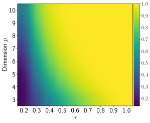
Figure 4: Evolution of $\rho(\mathcal{S}^{\tau})$ with varying values of ($\tau,p$).

A.4 Proof of Theorem 2

As stated in the introduction and in the preliminaries from Section 2, one can work with the angular measure $\Phi$ or the exponent measure $\mu$ in an equivalent way when studying the limit distribution of extremes. In this proof, we focus on the angular components $\theta_{i}$ induced by the normalization $\theta_{i}=\Theta(X_{i})=X_{i}/\|X_{i}\|_{\infty}$ so that the loss function is bounded in $[0,1]$. The proof relies on classical risk decompositions involving generalization and optimization errors. We have

$$\mathcal{R}_{t_{\gamma}}(\mathbf{W}_{mex})-\mathcal{R}_{t_{\gamma}}(\mathbf{W}_{t_{\gamma}}^{\star})=\underbrace{\left[\mathcal{R}_{t_{\gamma}}(\mathbf{W}_{mex})-\widehat{\mathcal{R}}_{k}(\mathbf{W}_{mex})\right]}_{generalization}+\underbrace{\left[\widehat{\mathcal{R}}_{k}(\mathbf{W}_{mex})-\widehat{\mathcal{R}}_{k}(\widehat{\mathbf{W}_{k}})\right]}_{optimization}+\underbrace{\left[\widehat{\mathcal{R}}_{k}(\widehat{\mathbf{W}_{k}})-\mathcal{R}_{t_{\gamma}}(\widehat{\mathbf{W}_{k}})\right]}_{generalization}+$$

$$\underbrace{\left[\mathcal{R}_{t_{\gamma}}(\widehat{\mathbf{W}_{k}})-\widehat{\mathcal{R}}_{k}(\widehat{\mathbf{W}_{k}})\right]}_{generalization}+\underbrace{\left[\widehat{\mathcal{R}}_{k}(\widehat{\mathbf{W}_{k}})-\widehat{\mathcal{R}}_{k}(\mathbf{W}_{t_{\gamma}}^{\star})\right]}_{\leq 0}+\underbrace{\left[\widehat{\mathcal{R}}_{k}(\mathbf{W}_{t_{\gamma}}^{\star})-\mathcal{R}_{t_{\gamma}}(\mathbf{W}_{t_{\gamma}}^{\star})\right]}_{generalization}.$$

Therefore,

$$\left|\mathcal{R}_{t_{\gamma}}(\mathbf{W}_{mex})-\mathcal{R}_{t_{\gamma}}(\mathbf{W}_{t_{\gamma}}^{\star})\right| \leq\left|\widehat{\mathcal{R}}_{k}(\mathbf{W}_{mex})-\widehat{\mathcal{R}}_{k}(\widehat{\mathbf{W}_{k}})\right|+\left|\mathcal{R}_{t_{\gamma}}(\mathbf{W}_{mex})-\widehat{\mathcal{R}}_{k}(\mathbf{W}_{mex})\right|+$$

$$\left|\mathcal{R}_{t_{\gamma}}(\widehat{\mathbf{W}_{k}})-\widehat{\mathcal{R}}_{k}(\widehat{\mathbf{W}_{k}})\right|+\left[\mathcal{R}_{t_{\gamma}}(\widehat{\mathbf{W}_{k}})-\widehat{\mathcal{R}}_{k}(\widehat{\mathbf{W}_{k}})\right]+\left|\mathcal{R}_{t_{\gamma}}(\mathbf{W}_{t_{\gamma}}^{\star})-\widehat{\mathcal{R}}_{k}(\mathbf{W}_{t_{\gamma}}^{\star})\right|,$$

Thus by taking the supremum over $\mathbf{W}$, on the latter term we finally obtain

$$\mathcal{R}_{t_{\gamma}}(\mathbf{W}_{mex})-\mathcal{R}_{t_{\gamma}}(\mathbf{W}^{\star}_{t_{\gamma}})\leq 4\sup_{\mathbf{W}}|\mathcal{R}_{t_{\gamma}}(\mathbf{W})-\widehat{\mathcal{R}}_{k}(\mathbf{W})|+|\widehat{\mathcal{R}}_{k}(\mathbf{W}_{mex})-\widehat{\mathcal{R}}_{k}(\mathbf{\widehat{W}}_{k})|$$ (9)

The right-hand side of the Eq. (9) is composed of two terms. The former, known as the generalization error, measures the gap between the true risk and its empirical counterpart whereas the latter is the optimization error between the solution $\mathbf{W}_{mex}$ found by MEXICO and the minimizer $\widehat{\mathbf{W}}_{k}$ of the empirical risk $\widehat{\mathcal{R}}_{k}$. The remainder of this proof relies on the following steps. We first provide a bound on the optimization error (Step 1) and then we upper-bound the generalization error (Step 2). This last term involves two quantities which are treated separately (Steps 2.1 and 2.2) on events with probability at least $(1-\delta/2)$. Collecting these two bounds and invoking the union bound concludes the proof (Step 3).

Step 1 - Optimization error $|\widehat{\mathcal{R}}_{k}(\mathbf{W}_{mex})-\widehat{\mathcal{R}}_{k}(\widehat{\mathbf{W}}_{k})|$. Up to rescaling the $\mathbb{M}$-set, the optimization error is bounded as follows:

$$|\widehat{\mathcal{R}}_{k}(\mathbf{W}_{mex})-\widehat{\mathcal{R}}_{k}(\widehat{\mathbf{W}}_{k})|\leq 2r_{\infty}^{p}(\tau).$$

For the sake of simplicity, assume that the columns of $\mathbf{W}_{mex}$ correspond to the columns of $\widehat{\mathbf{W}}_{k}$ for any cluster $K_{j}$ with $j\leq m$. Up to permutation of the columns, the former assumption may be withdrawn. We have

$$|\widehat{\mathcal{R}}_{k}(\mathbf{W}_{mex})-\widehat{\mathcal{R}}_{k}(\widehat{\mathbf{W}}_{k})|\leq\frac{1}{kp}\sum_{i=1}^{k}||\theta_{(i)}||_{1}||(\mathbf{W}_{mex}-\widehat{\mathbf{W}}_{k})^{\phi[(i)]}||_{\infty}\leq\frac{1}{k}\sum_{i=1}^{k}||(\mathbf{W}_{mex}-\widehat{\mathbf{W}}_{k})^{\phi[(i)]}||_{\infty}\leq 2r_{\infty}^{p}(\tau),$$

where we used that both mixture matrices belong to the $\mathbb{M}$-set $\mathcal{S}_{p}^{\tau}$.

Step 2 - Generalization error $\sup_{W}|\mathcal{R}_{t_{\gamma}}(\mathbf{W})-\widehat{\mathcal{R}}_{k}(\mathbf{W})|$. Recall that $k=\lfloor n\gamma\rfloor$ along with the formula of the empirical risk $\widehat{\mathcal{R}}_{k}(\mathbf{W})$ and consider the surrogate empirical risk $\widetilde{R}_{k}(\mathbf{W})$ defined by:

$$\widetilde{R}_{k}(\mathbf{W})=\frac{1}{k}\sum_{i=1}^{k}\ell(X_{(i)},\mathbf{W}),\qquad\widetilde{R}_{k}(\mathbf{W})\stackrel{{\scriptstyle\rm def}}{{=}}\frac{1}{k}\sum_{i=1}^{n}\ell(\theta_{i},\mathbf{W})\mathds{1}_{\{||X_{i}||_{\infty}\geq t_{\gamma}\}}$$

The generalization error may decomposed into

$$\mathcal{R}_{t_{\gamma}}(\mathbf{W})-\widehat{\mathcal{R}}_{k}(\mathbf{W})=\underbrace{\left[\mathcal{R}_{t_{\gamma}}(\mathbf{W})-\widetilde{R}_{k}(\mathbf{W})\right]}_{A}+\underbrace{\left[\widetilde{R}_{k}(\mathbf{W})-\widehat{R}_{k}(\mathbf{W})\right]}_{B}$$

Step 2.1 - Bound on A. The first term is bounded as follows

$$A =\mathcal{R}_{t_{\gamma}}(\mathbf{W})-\widetilde{R}_{k}(\mathbf{W})$$

$$={{\mathbb{E}}}\left[\ell(\Theta(X),W)\mid||X||_{\infty}\geq t_{\gamma}\right]-\frac{1}{k}\sum_{i=1}^{n}\ell(\theta_{i},\mathbf{W})\mathds{1}_{\{||X_{i}||_{\infty}\geq t_{\gamma}\}}$$

$$=\frac{1}{\gamma}{{\mathbb{E}}}\left[\ell(\Theta(X),W)\mathds{1}_{\{||X||_{\infty}\geq t_{\gamma}\}}\right]-\frac{1}{k}\sum_{i=1}^{n}\ell(\theta_{i},\mathbf{W})\mathds{1}_{\{||X_{i}||_{\infty}\geq t_{\gamma}\}}$$

$$=\left(\frac{1}{\gamma}-\frac{n}{k}\right){{\mathbb{E}}}\left[\ell(\Theta(X),W)\mathds{1}_{\{||X||_{\infty}\geq t_{\gamma}\}}\right]-\frac{1}{k}\sum_{i=1}^{n}\left(\ell(\theta_{i},\mathbf{W})\mathds{1}_{\{||X_{i}||_{\infty}\geq t_{\gamma}\}}-{{\mathbb{E}}}\left[\ell(\Theta(X),W)\mathds{1}_{\{||X||_{\infty}\geq t_{\gamma}\}}\right]\right)$$

Using that the loss $\ell(\cdot)$ is upper bounded by $1$ and ${{\mathbb{E}}}\left[\mathds{1}_{\{||X||_{\infty}\geq t_{\gamma}\}}\right]=\mathbb{P}(||X||_{\infty}\geq t_{\gamma})=\gamma$, we can bound the first term as

$$\left|\left(\frac{1}{\gamma}-\frac{n}{k}\right){{\mathbb{E}}}\left[\ell(\Theta(X),W)\mathds{1}_{\{||X||_{\infty}\geq t_{\gamma}\}}\right]\right|\leq\left|\left(\frac{1}{\gamma}-\frac{n}{k}\right)\gamma\right|\leq\frac{|k-n\gamma|}{k}\leq\frac{1}{k},$$

Therefore we have

$$|A|=\left|\mathcal{R}_{t_{\gamma}}(\mathbf{W})-\widetilde{R}_{k}(\mathbf{W})\right|\leq\frac{1}{k}+\frac{1}{k}\left|\sum_{i=1}^{n}\left(\ell(\theta_{i},\mathbf{W})\mathds{1}_{\{||X_{i}||_{\infty}\geq t_{\gamma}\}}-{{\mathbb{E}}}\left[\ell(\Theta(X),W)\mathds{1}_{\{||X||_{\infty}\geq t_{\gamma}\}}\right]\right)\right|.$$

We shall treat the last term with Bernstein inequality. Denote by $S_{n}=\sum_{i=1}^{n}U_{i}$ with $U_{i}=\ell(\theta_{i},\mathbf{W})\mathds{1}_{\{||X_{i}||_{\infty}\geq t_{\gamma}\}}$ and note that $\mathbb{E}[U_{i}]={{\mathbb{E}}}\left[\ell(\Theta(X),W)\mathds{1}_{\{||X||\geq t_{\gamma}\}}\right]$, $E_{n}=\sum_{i=1}^{n}\mathbb{E}[U_{i}]$, $V_{n}=\sum_{i=1}^{n}Var(U_{i})\leq n\gamma(1-\gamma)$.

Bernstein inequality implies, for $y>0$, $\mathbb{P}\left(|S_{n}-E_{n}|/k>y\right)\leq 2\exp\{-(y^{2}k^{2}/2)/(n\gamma(1-\gamma)+yk/3)\}:=\delta$. Solving the latter bound for $y$ yields $y=\frac{1}{k}\left(\frac{1}{3}\log(2/\delta)+\sqrt{(1/3\log(2/\delta))^{2}+2n\gamma(1-\gamma)\log(2/\delta)}\right)$. Simplifying the latter bound using that for $a,b>0$, $\sqrt{a+b}\leq\sqrt{a}+\sqrt{b}$, and that $n\gamma\leq k+1$, we obtain that with probability $1-\delta$,

$$|A|\leq\sqrt{\frac{2}{k}(1-\gamma)\log(2/\delta)}+\frac{1}{k}\left(\frac{2}{3}\log(2/\delta)+\sqrt{2(1-\gamma)\log(2/\delta)}+1\right)$$ (10)

Step 2.2 - Bound on B. The second term is bounded as follows

$$B =\widetilde{R}_{k}(\mathbf{W})-\widehat{R}_{k}(\mathbf{W})$$

$$=\frac{1}{k}\sum_{i=1}^{n}\ell(\theta_{i},\mathbf{W})\mathds{1}_{\{\|X_{i}\|_{\infty}\geq t_{\gamma}\}}-\frac{1}{k}\sum_{i=1}^{n}\ell(\theta_{i},\mathbf{W})\mathds{1}_{\{\|X_{i}\|_{\infty}\geq\|X_{(k)}\|_{\infty}\}}$$

$$=\frac{1}{k}\sum_{i=1}^{n}\ell(\theta_{i},\mathbf{W})\left[\mathds{1}_{\{\|X_{i}\|_{\infty}\geq t_{\gamma}\}}-\mathds{1}_{\{\|X_{i}\|_{\infty}\geq\|X_{(k)}\|_{\infty}\}}\right]$$

Again, using that the loss $\ell(\cdot)$ is upper bounded by $1$ and by triangle inequality we get

$$|B| \leq\frac{1}{k}\sum_{i=1}^{n}\left|\mathds{1}_{\{\|X_{i}\|_{\infty}\geq t_{\gamma}\}}-\mathds{1}_{\{\|X_{i}\|_{\infty}\geq\|X_{(k)}\|_{\infty}\}}\right|$$

To analyze this term, we shall consider whether $\|X_{(k)}\|_{\infty}\geq t_{\gamma}$ or not. We have

$$\sum_{i=1}^{n}\left|\mathds{1}_{\{\|X_{i}\|_{\infty}\geq t_{\gamma}\}}-\mathds{1}_{\{\|X_{i}\|_{\infty}\geq\|X_{(k)}\|_{\infty}\}}\right| =\begin{cases}\sum_{i=k+1}^{n}\mathds{1}_{\{\|X_{(i)}\|_{\infty}\geq t_{\gamma}\}}&\text{ if }\|X_{(k)}\|_{\infty}\geq t_{\gamma}\\ \sum_{i=1}^{k}\mathds{1}_{\{\|X_{(i)}\|_{\infty}<t_{\gamma}\}}&\text{ otherwise }\end{cases}$$

$$=\begin{cases}\sum_{i=1}^{n}\mathds{1}_{\{\|X_{(i)}\|_{\infty}\geq t_{\gamma}\}}-\frac{k}{k}&\text{ if }\|X_{(k)}\|_{\infty}\geq t_{\gamma}\\ \sum_{i=1}^{n}\mathds{1}_{\{\|X_{(i)}\|_{\infty}<t_{\gamma}\}}-\frac{n-k}{k}&\text{ otherwise }\end{cases}$$

$$=\left|\sum_{i=1}^{n}\mathds{1}_{\{\|X_{i}\|_{\infty}\geq t_{\gamma}\}}-1\right|$$

Therefore

$$|B|\leq\frac{1}{k}\left|\sum_{i=1}^{n}\mathds{1}_{\{\|X_{i}\|_{\infty}\geq t_{\gamma}\}}-1\right|$$

Denote by $S_{n}=\sum_{i=1}^{n}Z_{i}$ with $Z_{i}=\mathds{1}_{\{\|X_{i}\|_{\infty}\geq t_{\gamma}\}}$ and observe that $\mathbb{E}[S_{n}]=n\gamma$. We finally have

$$|B|\leq\frac{\left|S_{n}-n\gamma\right|}{k}+\frac{1}{k}$$

Similarly to the bound on A, we obtain that with probability $1-\delta$,

$$B\leq\sqrt{\frac{2}{k}(1-\gamma)\log(2/\delta)}+\frac{1}{k}\left(\frac{2}{3}\log(2/\delta)+\sqrt{2(1-\gamma)\log(2/\delta)}+1\right)$$ (11)

Step 3 - Final upper-bound. Using the union bound and combining the inequalities (10) and (11) from Steps 2.1 and 2.2, we obtain that with probability at least $(1-\delta)$,

$$\sup_{W}|\mathcal{R}_{t_{\gamma}}(\mathbf{W})-\widehat{\mathcal{R}}_{k}(\mathbf{W})|\leq\frac{1}{\sqrt{k}}2\sqrt{2(1-\gamma)\log(4/\delta)}+\frac{1}{k}\left(\frac{4}{3}\log(4/\delta)+2\sqrt{2(1-\gamma)\log(4/\delta)}+2\right),$$

and plug the bound on the optimization error (Step 1) into the decompostion (9) to conclude the proof.     

Appendix B Probabilistic Framework & Dependence of Extremes

B.1 On the Pareto Standardization $T$ and its Empirical Counterpart $\widehat{T}$

As the components of a random vector are not necessarily on the same scale, componentwise standardisation is a natural and necessary preliminary step. The Pareto standardization $T$ (and its empirical counterpart $\widehat{T}$) is mentionned in Algorithm 1. Following common practice in multivariate extreme value analysis (Beirlant et al., 2006), the input data $(X_{i})_{i\in\{1,\ldots,n\}}$ is standardised by applying the rank-transformation:

$$\widehat{T}(x)=\bigg{(}1/\Big{(}1-\widehat{F}_{j}(x)\Big{)}\bigg{)}_{j=1,\ldots,d}$$

for all $x=(x^{1},\ldots,x^{p})\in\mathbb{R}^{p}$ where $\widehat{F}_{j}(x)\stackrel{{\scriptstyle\rm def}}{{=}}\frac{1}{n+1}\sum_{i=1}^{n}\mathds{1}\{X_{i}^{j}\leq x\}$ is the $j^{th}$ empirical marginal distribution. Denoting by $\widehat{V}_{i}$ the standardized variables, $\forall i\in\{1,\ldots,n\},\widehat{V}_{i}=\widehat{T}(X_{i})$. The marginal distributions of $\widehat{V}_{i}$ are well approximated by standard Pareto distribution. The approximation error comes from the fact that the empirical c.d.f’s are used in $\widehat{T}$ instead of the genuine marginal c.d.f.’s $F_{j}$. After this standardization step, the selected extreme samples are $\{\widehat{V}_{i},\|\widehat{V}_{i}\|_{\infty}\geq V_{(\lfloor n\gamma\rfloor)}\}$.

B.2 Logistic distribution - An illustration of extremes dependence structure

The logistic distribution with dependence parameter $\delta\in(0,1]$ is defined in $\mathbb{R}^{p}$ by its c.d.f. $F(x)=\exp\big{\{}-(\sum_{j=1}^{p}{x^{(j)}}^{\frac{1}{\delta}})^{\delta}\big{\}}$. It can be considered as a simplified counterpart of the asymmetric logistic. Samples from both asymmetric logistic distribution and logstic distribution can be simulated according to algorithms proposed in Stephenson (2003). Figure 5 illustrates the logistic with various values of $\delta$. As $\delta$ gets close to $1$ extremes tend to occur in a non concomitant design, i.e. the probability of a simultaneous excess of a high threshold by more than one vector component is negligible. Conversely, as of $\delta$ gets close to $0$, extreme values are more likely to occur simultaneously.

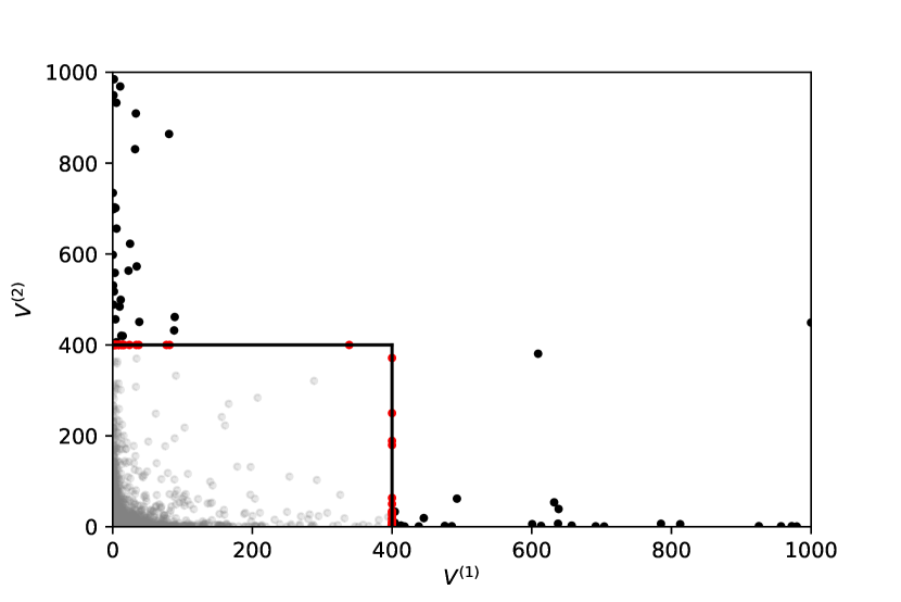
(a) low tail dependence

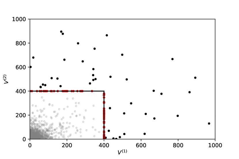
(b) moderate tail dependence

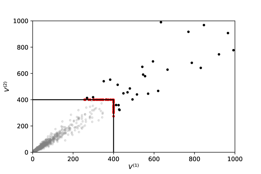
(c) high tail dependence

Figure 5: Illustration of the distribution of the angle $\Theta(X)$ obtained with bivariate samples $X$ generated from a logistic model with different coefficients of dependence ranging from near asymptotic independence 5(a) ($\delta=0.9$) to high asymptotic dependence 5(c) ($\delta=0.1$) including moderate dependence 5(b) ($\delta=0.5$). Non extreme samples are depicted in gray, extreme samples are represented with black dots and the angles $\Theta(X)$ (extreme samples projected on the $\ell_{\infty}$ sphere) are plotted in red. Note that not all extremes are shown since the plot was truncated for a better visualization. However all projections on the sphere are shown.

B.3 Structure Dependence

A common approach for modeling extreme events is to use some flexible parametric subclass of distributions (Stephenson, 2009). Let $F$ denote a multivariate extreme value c.d.f. Each univariate marginal distribution of $F$ is then a generalized extreme value distribution. More precisely, for $j\in\llbracket 1,p\rrbracket$, the $j$-th univariate marginal c.d.f is given by

$$F^{j}\left(x^{j}\right)=\exp\left[-\left(1+\xi_{j}\left(x_{j}-\mu_{j}\right)/\sigma_{j}\right)_{+}^{-1/\xi_{j}}\right]$$

where $\mu_{j},\xi_{j}$ and $\sigma_{j}>0$ are respectively the location, shape and scale parameters for the $j$-th marginal distribution.

The asymmetric logistic model provides perhaps the most popular parametric subclass of multivariate extreme value distributions. It is defined as follows.

Definition 4

(Asymmetric logistic, (Tawn, 1990)) Define $y_{j}=-1/\log F^{j}\left(x^{j}\right)$ for $j\in\llbracket 1,p\rrbracket$. The $p$-dimensional asymmetric logistic c.d.f is

$$F\left(x\right)=\exp\left[-\sum_{K\subset\llbracket 1,p\rrbracket}\left\{\sum_{j\in K}\left(\beta_{j,K}y_{j}\right)^{1/\alpha_{K}}\right\}^{\alpha_{K}}\right],$$

where $\alpha_{K}$ are the dependence parameters and $\beta_{j,K}$ are the asymmetry parameters.

Appendix C Self-supervised Learning

The task tackled in this paper revolves around understanding the dependence structure of extremes. At first glance, one may sum up our goal as a self-supervised learning problem where the objective would be to predict the $\ell_{1}$ norm of an extreme sample relying on subgroups of features best contributing to these features being extreme. Following Kolesnikov et al. (2019), given an extreme input $x$ one could build a preformulated label to be predicted as $||x||_{1}$, a regular linear regression model could be trained on the resulting trivial labeled dataset $\{(X_{(i)},Y_{(i)})\}_{i=1}^{k}$ with $Y_{(i)}=||X_{(i)}||_{1}$ and analyse the parameters of the linear regression model. Although, to the best of our knowledge there is no linear regression models which directly deals with non-predefined groups of features best contributing to the $\ell_{1}$ norm. For the sake of completeness we detail below the linear models involving such group analysis:

• Group Lasso (Yuan & Lin, 2006). The fomulation of our problem of interest as a group lasso supposes that the $p$ predictors are divided into $L$ groups, where $p_{l}$ represents the number of features in group $l$. The self-supervised learning problem rewrites as

  $$\min_{\beta_{l}\in\mathbb{R}^{p}}\left\|\|X\mathds{1}\|_{1}-\sum_{l=1}^{L}X_{l}\beta_{l}\right\|_{2}^{2}+\lambda\sum_{l=1}^{L}\sqrt{p_{l}}\|\beta_{l}\|_{2},$$

  where $\mathds{1}=(1,\ldots,1)^{T}$ denotes the column vector of size $k$ solely containing $1$ and $\lambda\in\mathbb{R}$. However, the group of features $L$ in the solution are predefined before solving the optimization problem. In that aspect, our framework differs from Group Lasso as we seek to find the groups of features.

• Sparse Group Lasso (Friedman et al., 2010). Sparse group lasso consists of a linear combination of group lasso and a lasso penalization that provide solutions that are both between and within group sparse. The minimization problem is the following

  $$\min_{\beta_{l}\in\mathbb{R}^{p}}\left\|\|X\mathds{1}\|_{1}-\sum_{l=1}^{L}X_{l}\beta_{l}\right\|_{2}^{2}+\tau\lambda\sum_{l=1}^{L}|\beta_{l}|+(1-\tau)\lambda\sum_{l=1}^{L}\sqrt{p_{l}}\|\beta_{l}\|_{2},$$ (12)

  where $\tau\in[0,1]$ balances the relative importance of sparsity term lasso or the group in the optimization problem. Although, in that setting the different groups of features still remain to be set in advance.

• Adaptive Group Lasso (Wang & Leng, 2008) & Adaptive Sparse Group Lasso (Mendez-Civieta et al., 2020).  Adaptive Group Lasso and Adaptive Sparse Group Lasso consist in setting a penalizations parameter $\lambda_{l}$ fot each features group $l\leq L$ in Eq. 12. Once again, the $L$ groups of features must be predefined and do no fit our setting as these groups are unknown and considering the total number of combination ($2^{p}-1$) could be computationally limiting as $p$ gets large.

Appendix D Numerical Experiments Details

D.1 Model Selection

DAMEX and Isolation Forest hyperparameters are the same as in Goix et al. (2016, 2017). Note that the performance of DAMEX and Isolation Forest in Table 6 differ from results from Table $4$ in Goix et al. (2016) since they report performance combining both the extreme and non-extreme regions: they rely on DAMEX for samples falling in the extreme regions and Isolation Forest on the non-extreme regions as they depict in their Figure 5. MEXICO parameters are set according to Remarks 2 and 4. Note that all performance reported in Tables 6 are solely computed on test samples considered as extreme since we focus on extreme regions.

D.2 Additional Results Feature Clustering

We present the full results of the performance of MEXICO regarding the feature clustering task. The projection step is either performed using alternating projections based on the method POCS (Projection Onto Convex Sets) or with the more elaborate technique Dykstra.

$p$	Spectral Clustering (Ding et al., 2005)			Spherical-Kmeans (Janßen et al., 2020)			MEXICO (POCS)
	H	C	v-M	H	C	v-M	H	C	v-M
75	0.925$\pm$0.054	0.937$\pm$0.040	0.931$\pm$0.046	0.950$\pm$0.034	0.972$\pm$0.024	0.961$\pm$0.027	0.978$\pm$0.025	0.976$\pm$0.024	0.977$\pm$0.024
100	0.918$\pm$0.058	0.934$\pm$0.039	0.926$\pm$0.048	0.943$\pm$0.031	0.967$\pm$0.024	0.955$\pm$0.026	0.976$\pm$0.020	0.979$\pm$0.021	0.976$\pm$0.020
150	0.889$\pm$0.060	0.925$\pm$0.031	0.906$\pm$0.045	0.940$\pm$ 0.026	0.962$\pm$0.020	0.951$\pm$0.022	0.973$\pm$0.015	0.977$\pm$0.013	0.975$\pm$0.014
200	0.886$\pm$0.047	0.928$\pm$0.024	0.906$\pm$0.034	0.940$\pm$0.018	0.962$\pm$0.014	0.951$\pm$0.015	0.970$\pm$0.015	0.975$\pm$0.012	0.972$\pm$0.013

Table 3: Comparison of Homogeneity (H), Completeness (C) and v-Measure (v-M) from prediction scores for Sppectral Clusterings Spherical-Kmeans and Mexico with alternating projections on simulated data with different dimension $p$.

$p$	Spectral Clustering (Ding et al., 2005)			Spherical-Kmeans (Janßen et al., 2020)			MEXICO (Dykstra)
	H	C	v-M	H	C	v-M	H	C	v-M
75	0.925$\pm$0.054	0.937$\pm$0.040	0.931$\pm$0.046	0.950$\pm$0.034	0.972$\pm$0.024	0.961$\pm$0.027	0.977$\pm$0.025	0.975$\pm$0.024	0.976$\pm$0.024
100	0.918$\pm$0.058	0.934$\pm$0.039	0.926$\pm$0.048	0.943$\pm$0.031	0.967$\pm$0.024	0.955$\pm$0.026	0.978$\pm$0.020	0.979$\pm$0.021	0.978$\pm$0.020
150	0.889$\pm$0.060	0.925$\pm$0.031	0.906$\pm$0.045	0.940$\pm$ 0.026	0.962$\pm$0.020	0.951$\pm$0.022	0.976$\pm$0.015	0.980$\pm$0.013	0.978$\pm$0.014
200	0.886$\pm$0.047	0.928$\pm$0.024	0.906$\pm$0.034	0.940$\pm$0.018	0.962$\pm$0.014	0.951$\pm$0.015	0.967$\pm$0.015	0.972$\pm$0.012	0.970$\pm$0.013

Table 4: Comparison of Homogeneity (H), Completeness (C) and v-Measure (v-M) from prediction scores for Spherical-Kmeans and Mexico with Dykstra projection on simulated data with different dimension $p$.

D.3 Additional Results on Anomaly detection

Real world data preprocessing.  We present the details about the preprocessing of the real world datasets.

Dataset	Size	Anomalies	$p$	$\tau$	$\lambda$
SF	73 237	3298 (4.5%)	4	0.8	10
SA	100 655	3377 (3.4%)	41	0.7	5
http	58 725	2209 (3.8%)	3	0.5	10
shuttle	49 097	3511 (7.2%)	9	0.7	5
forestcover	286 048	2747 (0.9%)	54	0.7	5

Table 5: Datasets Description and Parameter Configuration

The shuttle dataset is the fusion of the training and testing datasets available in the UCI repository (Lichman, 2013). The data have 9 numerical attributes, the first one being time. Labels from 7 different classes are also available. Class 1 instances are considered as normal, the others as anomalies. We use instances from all different classes but class 4, which yields an anomaly ratio (class 1) of 7.2%.

In the forestcover data, also available at UCI repository (Lichman, 2013), the normal data are the instances from class 2 while instances from class 4 are anomalies, other classes are omitted, so that the anomaly ratio for this dataset is 0.9%.

The last three datasets belong to the KDD Cup 99 dataset (KDDCup, 1999; Tavallaee et al., 2009), produced by processing the tcpdump portions of the 1998 DARPA Intrusion Detection System (IDS) Evaluation dataset, created by MIT Lincoln Lab (Lippmann et al., 2000). The artificial data was generated using a closed network and a wide variety of hand-injected attacks (anomalies) to produce a large number of different types of attack with normal activity in the background. Since the original demonstrative purpose of the dataset concerns supervised AD, the anomaly rate is very high (80%), which is unrealistic in practice, and inappropriate for evaluating the performance on realistic data. We thus take standard preprocessing steps in order to work with smaller anomaly rates.

For datasets SF and http we proceed as described in (Yamanishi et al., 2004): SF is obtained by picking up the data with positive logged-in attribute, and focusing on the intrusion attack, which gives an anomaly proportion of 4.5%. The dataset http is a subset of SF corresponding to a third feature equal to ’http’. Finally, the SA dataset is obtained as in (Eskin et al., 2002) by selecting all the normal data, together with a small proportion (3.4%) of anomalies.

Further Experimental details on Anomaly Detection. We present the full results of the performance of MEXICO regarding the anomaly detection task. The projection step is either performed using alternating projections based on the method POCS (Projection Onto Convex Sets) or with the more elaborate technique Dykstra.

Dataset	iForest (Liu et al., 2008)	DAMEX (Goix et al., 2016)	MEXICO (POCS)	MEXICO (Dykstra)
SF	0.381$\pm$0.086	0.710$\pm$0.031	0.892$\pm$0.013	0.710$\pm$0.030
SA	0.886$\pm$0.032	0.982$\pm$0.002	0.981$\pm$0.006	0.983$\pm$0.031
http	0.656$\pm$0.094	0.996$\pm$0.002	0.995$\pm$0.005	0.997$\pm$0.002
shuttle	0.970$\pm$0.020	0.990$\pm$0.003	0.990$\pm$0.003	0.989$\pm$0.003
forestcover	0.654$\pm$0.096	0.762$\pm$0.008	0.863$\pm$0.015	0.851$\pm$0.008

Table 6: Comparison of Area Under Curve of Receiver Operating Characteristic (ROC-AUC)from prediction scores of each method on different anomaly detection datasets.

Dataset	iForest (Liu et al., 2008)	DAMEX (Goix et al., 2016)	MEXICO (POCS)	MEXICO (Dykstra)
SF	0.393$\pm$0.081	0.650$\pm$0.034	0.812$\pm$0.016	0.661$\pm$0.031
SA	0.879$\pm$0.031	0.938$\pm$0.012	0.940$\pm$0.031	0.950$\pm$0.011
http	0.658$\pm$0.099	0.968$\pm$0.009	0.972$\pm$0.012	0.971$\pm$0.008
shuttle	0.826$\pm$0.055	0.864$\pm$0.026	0.864$\pm$0.037	0.818$\pm$0.024
forestcover	0.894$\pm$0.037	0.893$\pm$0.010	0.958$\pm$0.006	0.954$\pm$0.004

Table 7: Comparison of Average Precision (AP) from prediction scores of each method on different anomaly detection datasets.

Appendix E Further Numerical Experiments

E.1 MEXICO - Further Experimental Results

Cutler & Breiman (1994) provide an archetypal analysis of the Swiss Army dataset. This dataset consists of $6$ head dimensions from $200$ Swiss soldiers. The data was gathered to construct face masks for the Swiss army. Few samples of the dataset are presented in Table 8.

The first measurement (MFB) corresponds to the width of the face just above the eyes. The second feature (BAM) corresponds to the width of the face just below the mouth. The third measurement (TFH) is the distance from the top of the nose to the chin. The fourth feature (LGAN) is the length of the nose. The fifth measurement (LTN) is the distance from the ear to the top of the head while the sixth (LTG) is the distance from the ear to the bottom of the face. For a better visualization of the dataset, we made simple drawings of the different samples. Figure 6(a) illustrates the $6$ measurements.

id	MFB	BAM	TFH	LGAN	LTN	LTG
0	113.2	111.7	119.6	53.9	127.4	143.6
1	117.6	117.3	121.2	47.7	124.7	143.9
2	112.3	124.7	131.6	56.7	123.4	149.3
3	116.2	110.5	114.2	57.9	121.6	140.9
4	112.9	111.3	114.3	51.5	119.9	133.5

Table 8: Extract of the Swiss Army dataset.

A question that naturally rises is to figure out subgroups of face features that get large simultaneously. MEXICO algorithm performed on the standardized dataset provides the following groups of features : $\{5,6\}$(green), $\{1,3\}$(blue) and $\{2,4\}$(red), as illustrated in Figure 6(b). These results step in the direction of interpretability of feature clusters that may be large concomitantly in a real world dataset.

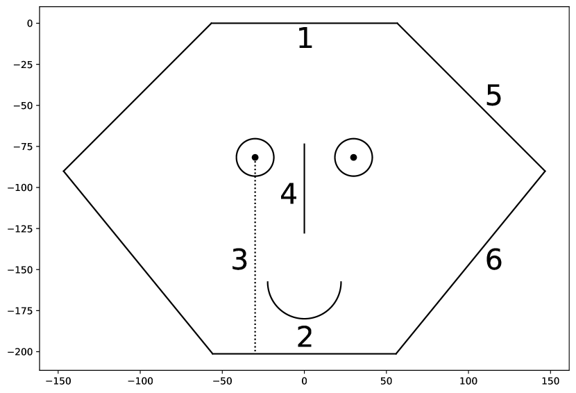
(a)

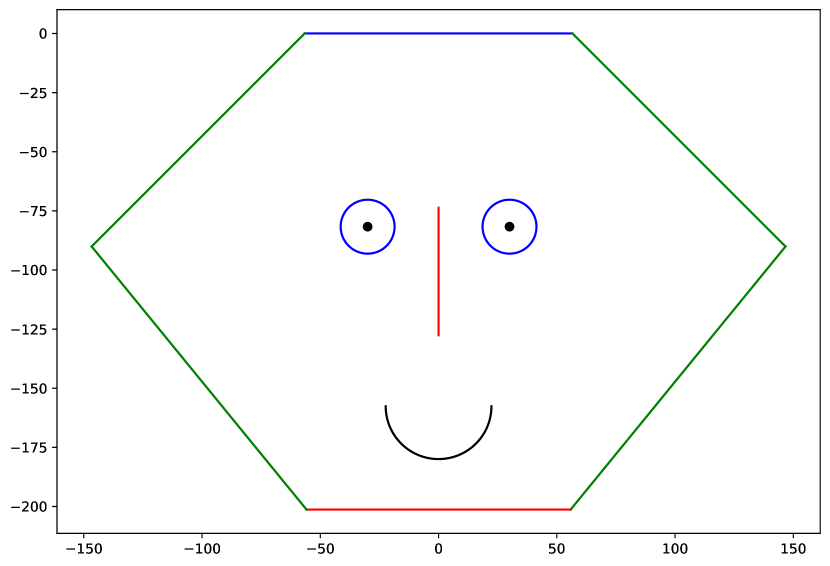
(b)

Figure 6: Illustration of the $6$ measurements (a) and subgroups that tend to be large simultaneously (b).

E.2 Classification in Extremes after Dimension Reduction.

In this section, we compare the influence on a downstream classification task of dimension reduction resulting from MEXICO and two other methods applied to extreme samples, namely PCA and Sparse PCA. The considered task is binary classification in extremes. Following the experiments from Jalalzai et al. (2018), we generate $5\cdot 10^{3}$ i.i.d samples in $\mathbb{R}_{+}^{4}$ following a logistic distribution with dependence parameter $\delta=0.2$. These points are labeled $+1$. Similarly we generate $5\cdot 10^{3}$ i.i.d samples in $\mathbb{R}_{+}^{4}$ following a logistic distribution with parameter $\delta=0.4$. These points are labeled $-1$. The samples are projected in lower-dimensional subspace according to methods summarized in Table 9. Random Forest is the considered class of classifiers. The number of trees is set to $10$. The norm is the $\ell_{\infty}$ norm. The value of $k$ is set to $100$. In Figure 7, boxplots obtained over $100$ runs show the test error rate in extremes for a Random Forest classifier after any dimension reduction method from Table  9.

Method	Initial dimension	Resulting dimension	Sparsity	Extreme Dependence Structure
PCA	$p$	$m$
Sparse PCA	$p$	$m$	✓
MEXICO	$p$	$m$	✓	✓

Table 9: Summary of Dimension Reduction Methods in Extremes.

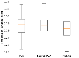
Figure 7: Classification Error in Extremes after Dimension Reduction.

E.3 Contraction mapping

Figure 8 depicts the contraction mapping property induced by MEXICO in the following example: Logistic data (see Section B.2 above) is generated in $\mathbb{R}^{4}$ with two different dependence structures $K_{1}=\{1,2\}$ and $K_{2}=\{3,4\}$ thus the total number of clusters $m$ is equal to $2$. The number of generated samples is $n=10^{6}$ and $k$ is set to $\sqrt{n}$. The violin plot on the left represents the distributional distance between $2$ standardized random extreme samples after normalization $\theta_{i}=X_{i}/\|X_{i}\|_{\infty},\theta_{2}=X_{2}/\|X_{2}\|_{\infty}$ while the violin plot on the right reports the distances between $2$ transformed and normalized data $\widetilde{\theta}_{i}=\widetilde{X}_{i}/\|\widetilde{X}_{i}\|_{\infty},\widetilde{\theta}_{2}=\widetilde{X}_{2}/\|\widetilde{X}_{2}\|_{\infty}$. All distances are computed on normalized data for the sake of visualization. The lower (resp. upper) part of the violin plot depicts the intra-cluster (resp. intra-cluster) $\ell_{2}$ distance.
First, We focus on the lower part of the violin plots: the distribution of intra-cluster distance is twice as big with the original data when compared to the transformed data. Second, it is worth noting that the inter cluster distances (i.e. upper part of the violin plot) tends to be smaller after transformation when compared with the original data.

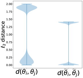
Figure 8: (Left)Violin plots of $l_{2}$ pairwise distances between normalized extreme samples $\theta_{i},\theta_{j}$ and (Right) corresponding pairwise distances for transformed samples $\widetilde{\theta}_{i},\widetilde{\theta}_{j}$.

E.4 Angular MEXICO

Theorem 2 provides a bound of the excess risk of MEXICO algorithm when working with normalized data. As suggested by the correspondance between the angular and exponent measures (see Definitions 2), the analysis of the dependence structure of extremes clusters of features with the normalized data (thus relying on the angular measure $\Phi$) is equivalent to the analysis with the non-normalized data (thus relying on the exponent measure $\mu$). Algorithm 2 is the counterpart of MEXICO as detailed in Algorithm 1 relying on the normalized extremes (i.e. $\{\Theta(X_{(i)})\}_{i\leq k}$). It follows Janßen et al. (2020) and exploits the normalized data to assess the dependence structure of extremes.

Input data or normalized data provide similar output matrix $\mathbf{W}_{mex}$ as illustrated in Figure 9 when dealing with the dataset detailed in Section E.3. The $\mathbf{W}_{mex}$ matrix associated to Algorithm 1 or Algorithm 2 both recovers the feature dependence structure of extremes as the first column of both matrices is associated to the cluster $\{0,1\}$ while the second column of both matrices is associated to the cluster $\{2,3\}$. Note that working on angular data implies normalizing samples which adds complexity to solve our problem of interest.

Algorithm 2 Angular MEXICO

0:  Training data $(X_{1},\ldots,X_{n}),0<m<p,\lambda>0$ and rank $k(=\lfloor n\gamma\rfloor)$.

1:  Initialize $(\mathbf{W}_{0},\mathbf{Z}_{0})\in\mathcal{A}_{p}^{m}\times\mathcal{A}_{m}^{n}$.

2:  Standardize the data $\widehat{V}_{(i)}=\widehat{T}(X_{(i)})$ (see Remark 1).

3:  Sort training data by decreasing order of magnitude $\|\widehat{V}_{(1)}\|_{\infty}\geq\ldots\geq\|\widehat{V}_{(n)}\|_{\infty}$.

4:  Consider the set of $k$ extreme training data $\widehat{V}_{(1)},\ldots,\widehat{V}_{(k)}$.

5:  Normalize the $k$ extreme data $\theta_{i}=\widehat{V}_{(i)}/\|\widehat{V}_{(i)}\|_{\infty}$.

6:  Compute $(\mathbf{W}_{mex},\mathbf{Z}_{mex})\in\mathop{\rm arg\,max}_{(\mathbf{W},\mathbf{Z})}f_{\lambda}(\mathbf{W},\mathbf{Z})$ using update rule (8) on the normalized data.

7:  Given a new input ${X}_{\text{new}}$ standardized as $\widehat{V}_{\text{new}}$ with $\|\widehat{V}_{\text{new}}\|_{\infty}\geq\|\widehat{V}_{(k)}\|_{\infty}$ and normalized as $\theta_{\text{new}}$compute $\widetilde{\theta}_{\text{new}}=\theta_{\text{new}}\mathbf{W}_{mex}$.

8:  Compute predicted cluster $\varphi_{0}=\mathop{\rm arg\,max}_{1\leq j\leq m}{\widetilde{\theta}_{\text{new}}^{j}}$.

9:  (FC) Return cluster $\varphi_{0}$. (AD) Return score $\ell(\widetilde{\theta}_{\text{new}},\mathbf{W}_{{mex}})$.

(a) MEXICO - Algorithm 1

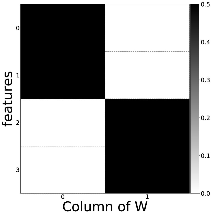
(b) Angular MEXICO - Algorithm 2

Figure 9: Matrix $\mathbf{W}_{mex}$ of Algorithm 1 (9(a)) and Algorithm 2 (9(b)).

Conclusions on experimental findings. Hereafter, we summarize the empirical findings detailed above:
First, working with extremes or their normalized counterparts provide similar results to estimate the support of extremes with MEXICO algorithm as illustrated in Section E.4. This empirical evidence is expected because of the one-to-one correspondance between the angular measure and the exponent measure. Second, while we make no claim that MEXICO outperforms PCA or Sparse PCA, it is worthy of attention that the dimension reduction induced by MEXICO remains competitive on a downstream classification task as detailed in Section E.2. Finally, the transformation induced by MEXICO can be considered as a contraction mapping as illustrated in Section E.3 for disjoint clusters. Future work will explore the analysis of MEXICO algorithm on overlapping clusters.

References

- Basrak et al. (2002) Basrak, B., Davis, R. A., and Mikosch, T. A characterization of multivariate regular variation. Annals of Applied Probability, pp. 908–920, 2002.
- Beirlant et al. (2006) Beirlant, J., Goegebeur, Y., Segers, J., and Teugels, J. L. Statistics of extremes: theory and applications. John Wiley & Sons, 2006.
- Bourbaki (2007) Bourbaki, N. Topologie générale: Chapitres 1 à 4. Springer Science & Business Media, 2007.
- Boyd & Wong (1969) Boyd, D. W. and Wong, J. S. On nonlinear contractions. Proceedings of the American Mathematical Society, 20(2):458–464, 1969.
- Boyle & Dykstra (1986) Boyle, J. P. and Dykstra, R. L. A method for finding projections onto the intersection of convex sets in hilbert spaces. In Advances in order restricted statistical inference, pp. 28–47. Springer, 1986.
- Bregman et al. (2003) Bregman, L. M., Censor, Y., Reich, S., and Zepkowitz-Malachi, Y. Finding the projection of a point onto the intersection of convex sets via projections onto half-spaces. Journal of Approximation Theory, 124(2):194–218, 2003.
- Calamai & Moré (1987) Calamai, P. H. and Moré, J. J. Projected gradient methods for linearly constrained problems. Mathematical programming, 39(1):93–116, 1987.
- Candès et al. (2006) Candès, E. J., Romberg, J., and Tao, T. Robust uncertainty principles: Exact signal reconstruction from highly incomplete frequency information. IEEE Transactions on information theory, 52(2):489–509, 2006.
- Candes et al. (2006) Candes, E. J., Romberg, J. K., and Tao, T. Stable signal recovery from incomplete and inaccurate measurements. Communications on Pure and Applied Mathematics: A Journal Issued by the Courant Institute of Mathematical Sciences, 59(8):1207–1223, 2006.
- Chautru (2015) Chautru, E. Dimension reduction in multivariate extreme value analysis. Electronic journal of statistics, 9(1):383–418, 2015.
- Chen & Ye (2011) Chen, Y. and Ye, X. Projection onto a simplex. arXiv preprint arXiv:1101.6081, 2011.
- Chiapino & Sabourin (2016) Chiapino, M. and Sabourin, A. Feature clustering for extreme events analysis, with application to extreme stream-flow data. In International Workshop on New Frontiers in Mining Complex Patterns, pp. 132–147. Springer, 2016.
- Chiapino et al. (2019) Chiapino, M., Sabourin, A., and Segers, J. Identifying groups of variables with the potential of being large simultaneously. Extremes, 22(2):193–222, 2019.
- Clifton et al. (2011) Clifton, D. A., Hugueny, S., and Tarassenko, L. Novelty detection with multivariate extreme value statistics. J Signal Process Syst., 65:371–389, 2011.
- Condat (2016) Condat, L. Fast projection onto the simplex and the ball. Mathematical Programming, 158(1):575–585, Jul 2016. ISSN 1436-4646. doi: 10.1007/s10107-015-0946-6. URL https://doi.org/10.1007/s10107-015-0946-6.
- Cooley & Thibaud (2019) Cooley, D. and Thibaud, E. Decompositions of dependence for high-dimensional extremes. Biometrika, 106(3):587–604, 2019.
- Cutler & Breiman (1994) Cutler, A. and Breiman, L. Archetypal analysis. Technometrics, 36(4):338–347, 1994.
- Daubechies et al. (2008) Daubechies, I., Fornasier, M., and Loris, I. Accelerated projected gradient method for linear inverse problems with sparsity constraints. journal of fourier analysis and applications, 14(5-6):764–792, 2008.
- De Haan & Ferreira (2007) De Haan, L. and Ferreira, A. Extreme value theory: an introduction. Springer Science & Business Media, 2007.
- Devijver et al. (2015) Devijver, E. et al. Finite mixture regression: a sparse variable selection by model selection for clustering. Electronic journal of statistics, 9(2):2642–2674, 2015.
- Ding et al. (2005) Ding, C., He, X., and Simon, H. D. On the equivalence of nonnegative matrix factorization and spectral clustering. In Proceedings of the 2005 SIAM international conference on data mining, pp. 606–610. SIAM, 2005.
- Drees & Sabourin (2019) Drees, H. and Sabourin, A. Principal component analysis for multivariate extremes. arXiv preprint arXiv:1906.11043, 2019.
- Duchi et al. (2008) Duchi, J., Shalev-Shwartz, S., Singer, Y., and Chandra, T. Efficient projections onto the l 1-ball for learning in high dimensions. In Proceedings of the 25th international conference on Machine learning, pp. 272–279. ACM, 2008.
- Dunn (1987) Dunn, J. C. On the convergence of projected gradient processes to singular critical points. Journal of Optimization Theory and Applications, 55(2):203–216, 1987.
- Dykstra (1983) Dykstra, R. L. An algorithm for restricted least squares regression. Journal of the American Statistical Association, 78(384):837–842, 1983.
- Embrechts et al. (1999) Embrechts, P., Resnick, S. I., and Samorodnitsky, G. Extreme value theory as a risk management tool. North American Actuarial Journal, 3(2):30–41, 1999.
- Embrechts et al. (2013) Embrechts, P., Klüppelberg, C., and Mikosch, T. Modelling extremal events: for insurance and finance, volume 33. Springer Science & Business Media, 2013.
- Engelke & Hitz (2018) Engelke, S. and Hitz, A. S. Graphical models for extremes. arXiv preprint arXiv:1812.01734, 2018.
- Engelke & Ivanovs (2020) Engelke, S. and Ivanovs, J. Sparse structures for multivariate extremes. arXiv preprint arXiv:2004.12182, 2020.
- Engelke et al. (2018) Engelke, S., De Fondeville, R., and Oesting, M. Extremal behaviour of aggregated data with an application to downscaling. Biometrika, 106(1):127–144, 12 2018. ISSN 0006-3444. doi: 10.1093/biomet/asy052. URL https://doi.org/10.1093/biomet/asy052.
- Eskin et al. (2002) Eskin, E., Arnold, A., Prerau, M., Portnoy, L., and Stolfo, S. A Geometric Framework for Unsupervised Anomaly Detection, pp. 77–101. Springer US, 2002.
- Friedman et al. (2010) Friedman, J., Hastie, T., and Tibshirani, R. A note on the group lasso and a sparse group lasso. arXiv preprint arXiv:1001.0736, 2010.
- Goix et al. (2016) Goix, N., Sabourin, A., and Clémençon, S. Sparse representation of multivariate extremes with applications to anomaly ranking. In Artificial Intelligence and Statistics, pp. 75–83, 2016.
- Goix et al. (2017) Goix, N., Sabourin, A., and Clémençon, S. Sparse representation of multivariate extremes with applications to anomaly detection. Journal of Multivariate Analysis, 161:12–31, 2017.
- Gubin et al. (1967) Gubin, L., Polyak, B. T., and Raik, E. The method of projections for finding the common point of convex sets. USSR Computational Mathematics and Mathematical Physics, 7(6):1–24, 1967.
- Jalalzai et al. (2018) Jalalzai, H., Clémençon, S., and Sabourin, A. On binary classification in extreme regions. In Advances in Neural Information Processing Systems, pp. 3092–3100, 2018.
- Jalalzai et al. (2020) Jalalzai, H., Colombo, P., Clavel, C., Gaussier, É., Varni, G., Vignon, E., and Sabourin, A. Heavy-tailed representations, text polarity classification & data augmentation. In Advances in Neural Information Processing Systems 33: Annual Conference on Neural Information Processing Systems 2020, NeurIPS 2020, December 6-12, 2020, virtual, 2020.
- Janßen et al. (2020) Janßen, A., Wan, P., et al. -means clustering of extremes. Electronic Journal of Statistics, 14(1):1211–1233, 2020.
- Jessen & Mikosch (2006) Jessen, H. A. and Mikosch, T. Regularly varying functions. Publications de l’Institut Mathematique, 80(94):171–192, 2006.
- Karamata (1933) Karamata, J. Sur un mode de croissance régulière. théorèmes fondamentaux. Bulletin de la Société Mathématique de France, 61:55–62, 1933.
- KDDCup (1999) KDDCup. The third international knowledge discovery and data mining tools competition dataset. 1999.
- Kolesnikov et al. (2019) Kolesnikov, A., Zhai, X., and Beyer, L. Revisiting self-supervised visual representation learning. In Proceedings of the IEEE/CVF Conference on Computer Vision and Pattern Recognition, pp. 1920–1929, 2019.
- Lee & Seung (2001) Lee, D. D. and Seung, H. S. Algorithms for non-negative matrix factorization. In Advances in neural information processing systems, pp. 556–562, 2001.
- Lichman (2013) Lichman, M. UCI machine learning repository, 2013. URL http://archive.ics.uci.edu/ml.
- Lippmann et al. (2000) Lippmann, R., Haines, J. W., Fried, D., Korba, J., and Das, K. Analysis and results of the 1999 darpa off-line intrusion detection evaluation. In RAID, pp. 162–182. Springer, 2000.
- Liu et al. (2008) Liu, F. T., Ting, K. M., and Zhou, Z.-H. Isolation forest. In 2008 Eighth IEEE International Conference on Data Mining, pp. 413–422. IEEE, 2008.
- Meilă (2006) Meilă, M. The uniqueness of a good optimum for k-means. In Proceedings of the 23rd international conference on Machine learning, pp. 625–632, 2006.
- Meilă (2007) Meilă, M. Comparing clusterings—an information based distance. Journal of multivariate analysis, 98(5):873–895, 2007.
- Mendez-Civieta et al. (2020) Mendez-Civieta, A., Aguilera-Morillo, M. C., and Lillo, R. E. Adaptive sparse group lasso in quantile regression. Advances in Data Analysis and Classification, pp. 1–27, 2020.
- Meyer & Wintenberger (2019) Meyer, N. and Wintenberger, O. Sparse regular variation. arXiv preprint arXiv:1907.00686, 2019.
- Niculae et al. (2018) Niculae, V., Martins, A. F., Blondel, M., and Cardie, C. Sparsemap: Differentiable sparse structured inference. arXiv preprint arXiv:1802.04223, 2018.
- Pedregosa et al. (2011) Pedregosa, F., Varoquaux, G., Gramfort, A., Michel, V., Thirion, B., Grisel, O., Blondel, M., Prettenhofer, P., Weiss, R., Dubourg, V., et al. Scikit-learn: Machine learning in Python. JMLR, 12:2825–2830, 2011.
- Resnick (1987) Resnick, S. Extreme Values, Regular Variation, and Point Processes. Springer Series in Operations Research and Financial Engineering, 1987.
- Resnick (1986) Resnick, S. I. Point processes, regular variation and weak convergence. Advances in Applied Probability, 18(1):66–138, 1986.
- Roberts (1999) Roberts, S. Novelty detection using extreme value statistics. IEE P-VIS IMAGE SIGN, 146:124–129, Jun 1999.
- Rosenberg & Hirschberg (2007) Rosenberg, A. and Hirschberg, J. V-measure: A conditional entropy-based external cluster evaluation measure. In Proceedings of the 2007 joint conference on empirical methods in natural language processing and computational natural language learning (EMNLP-CoNLL), pp. 410–420, 2007.
- Sabourin & Naveau (2014) Sabourin, A. and Naveau, P. Bayesian dirichlet mixture model for multivariate extremes: A re-parametrization. Comput. Stat. Data Anal., 71:542–567, 2014.
- Simon et al. (2013) Simon, N., Friedman, J., Hastie, T., and Tibshirani, R. A sparse-group lasso. Journal of computational and graphical statistics, 22(2):231–245, 2013.
- Stephenson (2003) Stephenson, A. Simulating multivariate extreme value distributions of logistic type. Extremes, 6(1):49–59, 2003.
- Stephenson (2009) Stephenson, A. High-dimensional parametric modelling of multivariate extreme events. Australian & New Zealand Journal of Statistics, 51:77–88, 2009.
- Tavallaee et al. (2009) Tavallaee, M., Bagheri, E., Lu, W., and Ghorbani, A. A detailed analysis of the kdd cup 99 data set. In IEEE CISDA, volume 5, pp. 53–58, 2009.
- Tawn (1990) Tawn, J. Modelling multivariate extreme value distributions. Biometrika, 77:245–253, 1990.
- Thomas et al. (2017) Thomas, A., Clemencon, S., Gramfort, A., and Sabourin, A. Anomaly detection in extreme regions via empirical mv-sets on the sphere. In AISTATS, pp. 1011–1019, 2017.
- Tipping & Bishop (1999) Tipping, M. E. and Bishop, C. M. Probabilistic principal component analysis. Journal of the Royal Statistical Society: Series B (Statistical Methodology), 61(3):611–622, 1999.
- Tsaig & Donoho (2006) Tsaig, Y. and Donoho, D. L. Extensions of compressed sensing. Signal processing, 86(3):549–571, 2006.
- Vignotto & Engelke (2018) Vignotto, E. and Engelke, S. Extreme value theory for open set classification–gpd and gev classifiers. arXiv preprint arXiv:1808.09902, 2018.
- Wang & Leng (2008) Wang, H. and Leng, C. A note on adaptive group lasso. Computational statistics & data analysis, 52(12):5277–5286, 2008.
- Wold et al. (1987) Wold, S., Esbensen, K., and Geladi, P. Principal component analysis. Chemometrics and intelligent laboratory systems, 2(1-3):37–52, 1987.
- Yamanishi et al. (2004) Yamanishi, K., Takeuchi, J.-I., Williams, G., and Milne, P. On-line unsupervised outlier detection using finite mixtures with discounting learning algorithms. Data Mining and Knowledge Discovery, 8(3):275–300, 2004.
- Yuan & Lin (2006) Yuan, M. and Lin, Y. Model selection and estimation in regression with grouped variables. Journal of the Royal Statistical Society: Series B (Statistical Methodology), 68(1):49–67, 2006.
- Şimşekli et al. (2015) Şimşekli, U., Liutkus, A., and Cemgil, A. T. Alpha-stable matrix factorization. IEEE Signal Processing Letters, 22(12):2289–2293, 2015.