1 Abstract

Two decades of U.S. government legislative outcomes, as well as the policy preferences of rich people, the general population, and diverse interest groups, were captured in a detailed dataset curated and analyzed by Gilens, Page et al. (2014). They found that the preferences of the rich correlated strongly with policy outcomes, while the preferences of the general population did not, except via a linkage with rich people’s preferences. Their analysis applied the tools of classical statistical inference, in particular logistic regression. In this paper we analyze the Gilens dataset using the complementary tools of Random Forest classifiers (RFs), from Machine Learning.

We present two primary findings, concerning respectively prediction and inference: (i) Holdout test sets can be predicted with approximately 70% balanced accuracy by models that consult only the preferences of rich people and a small number of powerful interest groups, as well as policy area labels. These results include retrodiction, where models trained on pre-1997 cases predicted “future” (post-1997) cases. The 20% gain in accuracy over baseline (chance), in this detailed but noisy dataset, indicates the high importance of a few wealthy players in U.S. policy outcomes, and aligns with a body of research indicating that the U.S. government has significant plutocratic tendencies.
(ii) The feature selection methods of RF models identify especially salient subsets of interest groups (economic players). These can be used to further investigate the dynamics of governmental policy making, and also offer an example of the potential value of RF feature selection methods for inference on datasets such as this.

2 Introduction

In 2014, Gilens and Page presented their ground-breaking paper “Testing Theories of American Politics: Elites, Interest Groups, and Average Citizens” [1], based on their research into the influence of various actors (power groups) on the outcome of important policy outcomes in the United States. The dataset spanned two decades, from 1981 to 2002, and consisted of policy cases determined to be of high importance. They identified and described an extensive array of independent variables in their paper and in their book “Affluence and Influence: Economic Inequality and Power in America” [2].

The two most important independent variables (hereafter “features”) outlined in their work were:

(i) The 90^th income percentile’s opinion (P90);

(ii) The net Interest Group Alignment (“netIGA”), a single derived variable combining the effects of 43 powerful interest groups (IGs).

They showed that public opinion at the 50^th percentile had little to no effect on the odds of policy adoption, challenging received notions of democracy in the United States.

Additional research over the years has further questioned notions of American democracy. Thomas Ferguson’s research into the effect of major investors and money on election outcomes has shown that money flows are an excellent predictor of U.S. congressional races outcomes [3] [4]. In 2016, the United States was downgraded by the UK-based Economic Intelligence Unit from“Full Democracy” to “Flawed Democracy” [5]. Bartel’s work has shown that the policy preferences of “affluent” Americans correlate closely with senators’ roll-call votes and government policy [6].

Gilens and Page applied classical methods of statistics and regression to analyse their dataset. Increasingly, Machine Learning (ML) methods are making their way into social science research [7], and offer a distinct, complementary approach and set of tools for dataset analysis, one focused on prediction rather than inference [8].

In the political sphere, ML methods have been applied to Supreme Court rulings [9], and to passage of bills in the U.S. Congress based on text in the bills [12, 10, 11]. Prediction does not require interpretability, and some ML methods are largely “black-boxes” (e.g. neural nets). But some ML methods (e.g. Random Forests) have interpretable aspects, and are thus potentially useful for inference [13].

Logistic regression (used by Gilens and Page) includes an intrinsic, strong assumption of linearity [14] (for details see Appendix). Random Forests (RFs) in contrast are flexible, non-linear classifiers [15] that can handle large numbers of sparsely-represented features such as the preferences of the 43 individual IGs in the Gilens dataset [16]. In addition, RFs have natural metrics to assess the relative importance of each feature. Thus RFs allow us to probe the dataset in complementary ways to Gilens and Page’s use of a calculated netIGA and logistic regression.

In this work we apply RF methods to the Gilens dataset with two goals, prediction and inference: We use RFs to build predictive models of U.S. policy; and we extend Gilens and Page’s inferential findings as to the influence of various actors on U.S. policy outcomes. We offer two main findings:
(i) Policy outcomes on holdout sets can be predicted with approximately 70% balanced accuracy (vs 50% chance baseline) using only a few feature categories from the Gilens dataset: Rich voters’ preferences, a subset (as few as 14 out of 43) of individual IGs’ preferences, and policy area labels.
(ii) The RF feature importance metrics enable further understanding and analysis of the salience of individual actors, and also provide an example of RFs’ potential usefulness for inference on datasets of this kind.

3 Methods

3.1 Dataset

The dataset consists of 1,836 major U.S. federal government policy cases dating from 1981 to 2002. In terms of prediction, the dependent variable $y$ is case outcome (“adopted” or “not adopted”). We reduced the large array of features in Gilens’ dataset to three primary categories, described below: (i) voter preferences (in particular, of the wealthy) (ii) IG alignments, and (iii) policy descriptors (such as “Foreign”, “Social Welfare”, etc). Corresponding abbreviations are listed in Table 1.

Table 1: Feature abbreviations

P90	Voter preference of 90th income %ile
netIGA	Net Interest Group Alignment
IGs	Individual Interest Groups (preferences)
PAs	Policy Areas
PDs	Policy Domains (a coarser version of PAs)

Voter preferences (P90):

Preferences of different wealth tranches were obtained from national surveys of the general public, where participants were asked whether they favored or opposed a proposed policy change. Preferences of the different wealth tranches were then imputed at various income percentiles, viz 90^th, 50^th, and 10^th (hereafter P90, P50, P10). Gilens and Page noted that P90 was a (rough) indicator of the preferences of even higher income percentiles (e.g. P99). One of their key findings was that, among voter preferences, only P90 impacted case outcomes. Our models used P90 as the sole voter preference feature (use of P50 or P10 as features degraded model accuracy).

Interest groups (IGs and netIGA):

The dataset includes alignments, on each case, for a total of 43 distinct IGs. These IGs were mostly business groups such as the American Bankers Association, and also some social IGs such as the AARP (American Association of Retired Persons). The alignment of each IG toward each case was assigned an ordinal value between 2 and -2 (Strongly Support, Somewhat Support, Neutral, Somewhat Oppose, or Strongly Oppose). Routinely, a given IG had no opinion in a particular case, so non-neutral (non-zero) values were sparse.

To aid their analysis, Gilens and Page combined the alignments of all the individual IGs to create a single feature, the “netIGA” as follows:

$$\text{netIGA}=log(F_{2}+0.5F_{1}+1)~{}-~{}log(O_{2}+0.5O_{1}+1),\text{ where}$$ (1)

$F_{2}$ = number of IGs strongly in favor, $F_{1}$ = number somewhat in favor, $O_{2}$ = number strongly opposed, and $O_{1}$ = number somewhat opposed. The $log(~{})$ accounts for diminishing effects of multiple IGs weighing in on the same side of a given case.

Because RFs readily handle large numbers of features, we set aside the netIGA and instead used each IG’s alignment value as a separate feature.

Policy areas (PAs):

The Gilens dataset includes an in-depth policy descriptor category which we refer to as policy area (PA) labels, e.g. Campaign Finance, Welfare Reform, etc.

A full list of the 19 PAs is given in the Appendix. PAs were expressed as features via one-hot encoding (i.e. one feature per PA, taking values 0 or 1, according as the case was in that PA). Each case is assigned to exactly one PA.

Policy Domains (PDs):

The Gilens dataset also includes six broader policy domain (PD) labels (Economic, Foreign, Social welfare, Religious, Guns, and Miscellaneous). In general, several PAs are contained in one PD, though some PAs are also PDs (e.g. Foreign Policy). PDs were one-hot encoded. Table 2 shows a breakdown of positive (i.e. adopted) and negative (i.e. not adopted) cases by PD over the full dataset, as well as over just the post-1997 test set (used for retrodiction).

PDs were used for feature selection: We grouped cases by PD, trained a different RF model for each PD using P90 and individual IGs as features, then selected the most salient IGs for each PD based on these models.

Table 2: Positive and negative case counts. Number of positive (“adopted”) and negative (“not adopted”) cases, as well as percentage of cases that were positive, for each PD, over the full dataset (numbers over post-1997 cases are in parentheses). Economic policy and Foreign policy are fairly evenly-balanced, while other PDs skew negative. In some PDs (e.g. Social Welfare, Guns) the distribution of positive/negative cases differed pre- vs post-1997.
 

Domain	Pos	Neg	%Pos
Economic	160 (36)	248 (38)	39% (49%)
Foreign	244 (77)	196 (59)	55% (57%)
Social Welfare	101 (20)	310 (152)	25% (12%)
Religious	43 (18)	123 (68)	26% (21%)
Guns	18 (1)	81 (49)	18% (2%)
Misc	77 (36)	235 (95)	25% (27%)
Total	643 (188)	1193 (461)	35% (29%)

3.2 Train/test splits

We trained models in two regimes: (i) Random train/test splits drawn from the full dataset ( N = 25 draws, ratio 67%, 33%). This provided robust error bars on our prediction accuracy results since each train/test split was different. (ii) Future prediction (more precisely, retrodiction): All pre-1997 cases in training and all post-1997 cases (including 1997) in testing (ratio 65%, 35%).

Retrodiction tested stability over time, with the possibility that individual IGs might gain or lose relevance over the two decade duration of the dataset.

3.3 Reported metrics

We report two figures of merit: maximum Balanced Accuracy, and Area Under the Curve (AUC) of the ROC curve. Evaluated on the test set, these are standard measures of a model’s classifying abilities. Maximum balanced accuracy is defined as

$$balanced~{}accuracy=\frac{sensitivity+specificity}{2},$$ (2)

where sensitivity is the percentage of positive cases correctly classified, and specificity is the percentage of negative cases correctly classified. The operating point (decision threshold) used to predict test cases is that which gives maximum balanced accuracy on the training set (this threshold typically gives lower test set accuracy than would be possible given oracle knowledge of test set behavior).

We report balanced rather than raw accuracy for two reasons. First, it has a clear, consistent baseline accuracy (50% = chance). Second, in this dataset, negative cases outnumber positive ones, by substantial margins in some policy domains (cf. Table 2). Given a class imbalance, raw accuracy blurs the differences between models because all models can leverage the imbalance by effectively betting on system inertia (i.e. the fact that most legislation is not adopted).

3.4 Random Forest models

RFs are flexible, robust, non-linear classifiers [15] based on ensembles of decision trees. In a RF, many decision trees are generated, each of which trains on a random subset of the training data. At each node of a given tree, a randomly-chosen feature splits the data. The final prediction of a test case is an average of the trees’ predictions of that case. RFs are adept at handling sparse datasets with large number of features [16], though removing uninformative features can improve model accuracy.

Our code was written in Python [17] and used the sklearn library [18]. Full codebase can be found at [19].

The accuracies of two other flexible classifiers, XGBoost [20] (a flavor of RF) and Neural Nets, were similar to standard RFs (results not reported).

3.5 Feature selection

To rank the importance of the various IGs as features, cases were divided into 6 groups according to Policy Domain. For each domain, RFs were trained on random train/test splits (N = 21), using P90 and the 43 IGs as features. The averaged feature importance scores were then ranked. For more details see the Appendix.

4 Results

Results are divided into two sections: Inference (feature selection by RFs); and Prediction (including retrodiction).

4.1 Inference

The goal of Inference was to identify the most salient IGs by ranking their power as predictors. The 43 IGs were ranked as predictors for each Policy Domain as described above. A typical feature ranking (for the Foreign Policy domain) is shown in Table 3. Similar tables of IG rankings for other PDs are in the Appendix.

The ranking extracted those IGs with the most impact on policy outcomes, which has direct relevance to the study of policy decision-making in the U.S. We note three points about the rankings:

(1) Saliency (defined as maximizing model accuracy) is not the same as effectiveness of influence, because an IG’s success is also a function of the difficulty of the particular cases it lobbied for or against (by analogy, a baseball player’s batting average is partly a function of the pitchers they face).

(2) Bias can be introduced into the rankings based on various predictor attributes [22]. For example, less-sparse features (IGs with more at-bats) tend to have higher rankings. In this dataset, restricting by Policy Domain mitigates this difference in sparsity since IGs tend to be especially active in a particular PD.

(3) An IG can have predictive saliency due to negative correlations.

Correlations between IG preferences and case outcomes are given in Column 3 of Table 3. To calculate this correlation, only cases where the IG was not neutral (i.e. was “at bat”) were considered:

$$corr(IG)=\frac{0.5}{\#at~{}bats}\left(\sum\limits_{i|y_{i}=1}x_{i}~{}-\sum\limits_{i|y_{i}=0}x_{i}\right),\text{ where }$$ (3)

$x_{i}$ = IG preference $\in${ -2, -1, +1, +2} and $y_{i}$ = outcome $\in${ 0 or 1}, for the i^th case. The 0.5 term normalizes the IG preference values. For these calculations, P90 values were rescaled from [0,1] to [-2, 2] and then values in [-0.4, 0.4] (i.e. noncommittal) were set to 0, to allow comparison with IGs.

Table 3: Feature importance scores in Foreign policy. Feature importance scores, IG stance vs case outcome correlations, and IG at-bats, given as mean $\pm$ std dev over 25 random train/test splits of the full dataset, restricted to Foreign policy cases only. “at-bats” gives the number of test cases for which the IG had a non-neutral stance (out of 147 $\pm$ 7 foreign policy test cases).

	RF	IG-outcome	at-bats
IG	score	correlation	(out of 147)
P90	41 $\pm$ 3	20 $\pm$ 3	93 $\pm$ 6
Defense industry	12 $\pm$ 3	41 $\pm$ 13	39 $\pm$ 5
AIPAC	7 $\pm$ 2	-18 $\pm$ 11	17 $\pm$ 4
Auto companies	5 $\pm$ 1	48 $\pm$ 15	13 $\pm$ 2
UAW union	5 $\pm$ 1	-59 $\pm$ 14	41 $\pm$ 3
Oil companies	4 $\pm$ 1	37 $\pm$ 33	5 $\pm$ 2
Airlines	4 $\pm$ 1	54 $\pm$ 23	8 $\pm$ 2

Columns 2 and 3 are scaled by 100$\times$.

For example, in the Foreign policy domain (cf Table 3, Defense Contractors’ stance was positively correlated with outcomes (mean $\pm$ std dev: 41 $\pm$ 13), AIPAC’s stance had mixed correlation (18 $\pm$ 11), and Labor Unions’ stances were negatively correlated (-59 $\pm$ 14). Note that negative correlation does not mean that the IG “lost”: Its actions may have averted worse outcomes, or modified the case’s legislative details in desired ways.

The most salient IGs for each Policy Domain, as determined by RF feature selection, were as follows:
1. Foreign policy: Defense contractors; then AIPAC, auto companies and auto workers union.
2. Economic policy: Construction and realtors; then tobacco companies and a union.
3. Social welfare policy: the AARP and investment companies; then governors, pharmaceutical companies, universities, teachers, and health insurance companies.
4. Religious policy: Christian and anti-abortion groups; then doctors, teachers, beer companies, tobacco companies, health insurance companies, and broadcasters.
5. Gun policy: the NRA (no other IG was active).
6. Miscellaneous: Chamber of Commerce; then two unions (AFL-CIO and government workers), automobile companies; then oil companies, Christian Coalition, and trial lawyers.
The preferences of the wealthy (P90) outranked every IG in every policy domain except Social Welfare, where the AARP dominated.

Tables of IG data for each Policy Domain (feature importance, correlations with outcomes, and number of “at-bats”) are given in the Appendix.

4.1.1 Advantages of RF’s nonlinear flexibility in feature selection

RFs do not have the built-in linear structure of logistic regression. In the inference context, this flexibility means that RFs can give insights into feature salience which are unavailable to logistic regression.

An example from the foreign policy domain data is described here. The highest ranked features for the RF model were P90 and Defense Contractors. The logistic regression model for the foreign policy domain ranked P90 and Defense Contractors as the 2nd and 6th most salient features, respectively. We examined policy cases involving P90 and Defense Contractors to gain some comparative understanding.

When Defense Contractors strongly favor a policy change, they almost always get their way, even when the wealthy are opposed. However, when the Defense Contractors oppose a policy change, P90 has a strong positive correlation with outcomes. Logistic regression fails to parse this effect, giving many False Negatives (see Fig 1). RFs handle this readily, yielding 95% balanced accuracy for the RF vs 79% for logistic regression. That is, the high importance of P90 in Foreign policy cases depends on a relationship more readily encoded by the RF model.

We note that RFs selected significantly more salient features than did logistic regression. For details see the Appendix, section 6.2.

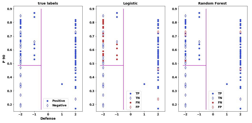
Fig 1: Benefit of nonlinear splits. Foreign policy outcomes on cases where Defense Contractors had a non-neutral stance. y-axis = P90, x-axis = Defense Contractors’ preference. Solid dots are positive outcomes, open diamonds are negatives. TP = true positive, TN = true negative, FN = false negative, FP = false positive. left: True outcomes. There are three regions, marked by magenta lines: When Defense Contractors favored a case it almost always passed, regardless of P90 (right half of plot). When Defense Contractors opposed a case then either: it failed if P90 opposed it (lower left) or it had reasonable odds of passing if P90 favored it (upper left). middle: Logistic predictions (blue = correct, red = wrong), with many errors in the upper left region. right: RF predictions (blue = correct, red = wrong). RFs readily parse all three regions.

4.2 Prediction

The goal of Prediction was to examine to what degree U.S. legislative outcomes might be predicted from the preferences of rich voters and Interest Groups, and which actors were most informative.

Our key finding is that legislative outcomes can be accurately predicted using P90, policy descriptors (PDs or PAs), and individual IGs. Balanced accuracy on test sets of the trained RF reached $\approx$70%, a gain of 20% over baseline chance.

P90 was a vital feature, in the sense that excluding it always degraded accuracy. Inclusion of P50 (median wealth voter preferences) as a feature slightly degraded accuracy, consistent with the finding of P50’s irrelevance in [1]. Use of either PD or PA labels as a feature increased accuracy. Training and then combining separate models for each Policy Domain did not increase overall accuracy (results not reported).

We report results for RF models using four feature sets (listed below), in two train/test scenarios: (i) Multiple random train/test splits of the full dataset (“Random Draw” in Table 4); and (ii) Retrodiction (i.e., train on pre-1997 cases and test on post-1997 cases, a single train/test split).

Feature sets used were:

Set A: P90 and netIGA (Baseline, from [1]).

Set B: P90, PDs, and all 43 individual IGs.

Set C: P90, PDs, and 14 IGs chosen by RF feature selection (Gini impurity).

Set D: P90, PAs, and all 43 IGs.

Balanced accuracies and AUCs for RF models using the four Feature Sets and in the two regimes are given in Table 4. We offer the following observations:

(1) All feature sets used P90, which was always the most important. The feature sets differed in how they used IGs, and how they used Policy descriptors.

(2) Sets B - D substantially outperformed Set A (e.g. 11% mean increase in AUC).
Use of individual IGs vs the simplified netIGA was the main factor behind this improvement in prediction accuracy. Figure 2 shows the mean improvement in accuracy of Set B over Set A, broken out by individual IGs (“Random Draw” regime).

(3) Set C had equivalent performance to Set B, indicating that a small subset of 14 IGs (chosen by RF feature selection) carried as much salience as the full set of 43 IGs. We note this does not imply that these 14 IGs were the only ones that mattered: Certainly they were important actors, but they likely also encoded correlated salience of other IGs.

(4) Set D posted better performance than Model B, indicating that Policy Area labels had more salience than the coarser Policy Domain labels.

(5) Set D gave the best results (70% balanced accuracy, 78% AUC). The full list of features for Model D, with their importance rankings, is given in Table 10 in the Appendix.

Table 4: RF accuracy with various feature sets. Balanced Accuracy and AUC for RFs given various feature sets. “PD” means Policy Domains. “PA” means Policy Areas. Results are given as percentages, mean $\pm$ 1 std dev (N = 25).

Model	Random Draw		Retrodiction
	Bal Acc %	AUC %	Bal Acc %	AUC %
A: P90, netIGA	61.5 $\pm$ 1.7	66.2 $\pm$ 2.1	64.6 $\pm$ 0.6	70.2 $\pm$ 0.3
B: P90, 43 IGs, PDs	67.3 $\pm$ 1.6	74.9 $\pm$ 1.7	69.0 $\pm$ 0.7	75.7 $\pm$ 0.2
C: P90, 14 IGs, PDs	67.3 $\pm$ 1.6	75.1 $\pm$ 1.6	68.8 $\pm$ 0.5	75.7 $\pm$ 0.2
D: P90, 43 IGs, PAs	70.1 $\pm$ 1.5	77.7 $\pm$ 1.5	71.3 $\pm$ 0.7	76.5 $\pm$ 0.4

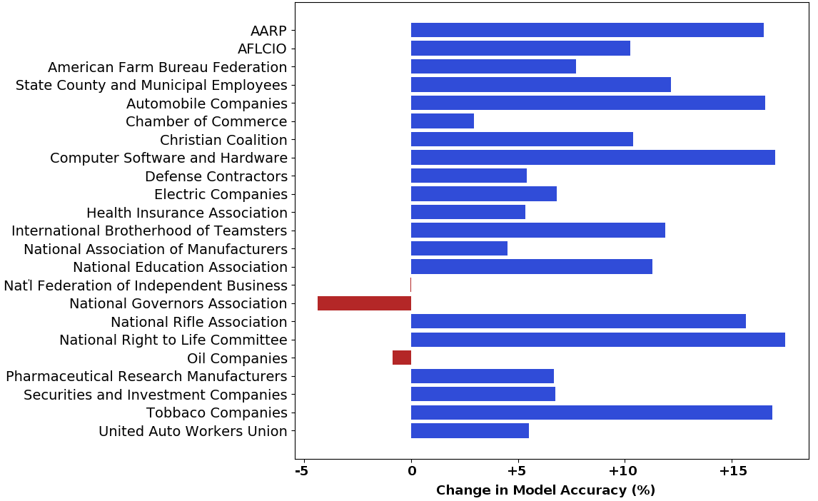
Fig 2: Gain in accuracy per IG, Set B vs Set A. Set B used P90, all 43 IGs and Policy Domains. Set A used P90 and netIGA only. For each IG, we measured test set accuracy on those cases where the IG was “strongly in favor” or “strongly opposed” and plotted accuracy(Set B) - accuracy(Set A). Set B consistently improved accuracy on these IG-based groups of cases. Random draw regime, N = 25. Each IG shown had at least 20 cases in the test set.

5 Discussion

In this work we applied the tools of Machine Learning to the Gilens dataset, as an aid to inference as well as for prediction. RF algorithms readily handle sparse datasets that can be difficult for traditional regression techniques. RF methods enabled prediction of policy outcomes with surprising accuracy, especially considering the intrinsic noisiness of the dataset. They also enabled us to examine the role of individual IGs and the effects of various features of the dataset. Additionally, we have shown how RFs can provide insights into feature saliency distinct from and arguably superior to traditional regresssion techniques such as logistic regression.

We found that case outcomes on test sets were predictable with $\approx$70% balanced accuracy using only the preferences of the wealthy (P90), individual Interest Groups, and Policy Area labels as features. Inclusion of the wishes of median income voters (P50) always reduced predictive accuracy. These results also held for a retrodiction split, training on pre-1997 cases and testing on post-1997 cases. We believe that the high predictability of policy outcomes using models based on only a few wealthy actors (P90 and certain IGs) reinforces Gilens and Page’s findings about the plutocratic tendencies of U.S. government.

We suspect that the 90^th percentile serves as a proxy for the opinions of the very wealthy, and we expect that predictive accuracy would further improve given better measures of the opinions of the “very wealthy” (e.g. the 99^th income percentile).

There has been effort in recent years to capture the policy opinions of the very wealthy as distinct from the general population. A unique study led by Benjamin Page effectively captured, via surveys and interviews, the policy preferences of those in, or near, the top 1% of income in the United States [24]. The results indicated, among other things, that the very wealthy held policy preferences that were much more conservative in such important domains as social welfare programs, taxation, and regulation of the economic system. Their research also showed that the very wealthy were much more politically active, with significantly higher rates of financial contributions to, and contact with, public officials. This highlights the importance of quantitatively capturing the opinions of the very wealthy in the future, in order to better understand their impact on policy adoption by the U.S. government.

6 Appendix

6.1 Logistic regression

Given a feature-label pair {$\bm{x},y$}, logistic regression gives an estimate $\hat{y}$ of the class $y$, using features $\bm{x}$, by passing a linear combination of feature values $\bm{\beta x}$ through a (non-linear) sigmoid function $\sigma(s)=\frac{1}{1-e^{-s}}$. The coefficients $\bm{\beta}$ are the fitted parameters.

$$\hat{y}=\frac{1}{1-e^{-\bm{\beta x}}}$$ (4)

6.2 Feature selection details

In order to identify the most important IGs, we used RF’s standard Gini impurity method [21], indicated for this dataset because the features were sparse, non-categorical, and similarly scaled (in range [-2, 2]) [16] (because IGs were ranked for each Policy Domain separately, the PDs were not features.)

For feature ranking purposes, P90 scores were rescaled from [0,1] to [-2, 2] to match the IG preference range. Unlike Gini impurity, RF’s Permutation method had unstable results (IG rankings changed if P90 was excluded). In general, the RFs selected different subsets of important IGs than those selected via the $\beta$ coefficients of logistic regression.

Features selected by RF (Gini impurity) significantly out-performed features selected by logistic regression, in the sense that using RF-Gini features gave a model (either RF or logistic regression) much higher accuracy than using features selected by logistic regression. Features chosen by FR’s Permutation method landed between the two. Table 5 shows the gain in accuracy due to RF (Gini)-chosen features vs logistic-chosen features.

We note that for a fixed set of features, RF and logistic regression models gave similar accuracies (in general, RF accuracy was slightly but not significantly better, consistent with [23]). The key advantage of RFs lay not in prediction per se, but rather in selecting much more salient features (i.e. inference).

Table 5: Difference in salience of IGs chosen by RF vs logistic regression. Balanced accuracy (balAcc) and AUC of RF and logistic models on test sets, using either RF-chosen IGs or logistic-chosen IGs, given as mean $\pm$ std dev. The gains in accuracy (RF-chosen minus Logistic-chosen) are shown in bold. (N= 21 train/test splits).

Setup		Full data		Retrodiction
Model	IG type	balAcc	AUC	balAcc	AUC
	RF-chosen (Gini)	63.5 $\pm$ 1.6	68.2 $\pm$ 2.2	66.4 $\pm$ 2.4	69.7 $\pm$ 1.0
RF	Logistic-chosen	56.7 $\pm$ 1.7	61.1 $\pm$ 1.9	53.4 $\pm$ 2.7	53.9 $\pm$ 2.7
	Gain	6.8 $\pm$ 1.9	7.0 $\pm$ 1.6	13.0 $\pm$ 4.4	15.8 $\pm$ 3.3
	RF-chosen (Gini)	59.5 $\pm$ 1.8	61.4 $\pm$ 2.1	59.3	62.6
Logistic	Logistic-chosen	55.0 $\pm$ 1.6	56.6 $\pm$ 1.6	52.6	51.6
	Gain	4.5 $\pm$ 1.9	4.7 $\pm$ 1.7	6.7	10.9

“Gain” is the mean of differences (not difference of means).

Logistic regression is deterministic on non-separable data, so its prediction of the post-1997 data has 0 std dev.

6.3 IG rankings by Policy Domain

Importance rankings, correlations with case outcomes, and number of “at-bats” for IGs, for various Policy Domains, are given in Tables 6 - 9. For more details, and for a table of Foreign policy results, see section 4.1.

Table 6: Economic policy. Correlations for the most salient IGs, given as mean $\pm$ std dev. Each test set had 130 $\pm$ 6 Economics cases.

	RF	IG-outcome	at-bats
IG	score	correlation	(out of 130)
P90	21 $\pm$ 2	12 $\pm$ 4	94 $\pm$ 5
Nat’l Assoc Homebuilders	6 $\pm$ 2	23 $\pm$ 7	41 $\pm$ 5
Nat’l Assoc Realtors	6 $\pm$ 2	46 $\pm$ 11	22 $\pm$ 4
Tobacco Companies	5 $\pm$ 1	18 $\pm$ 11	31 $\pm$ 6
Teamsters union	5 $\pm$ 1	40 $\pm$ 11	19 $\pm$ 3

Columns 2 and 3 are scaled by 100$\times$.

Table 7: Social Welfare policy. Correlations for the most salient IGs, given as mean $\pm$ std dev. The AARP had strong positive correlation with outcomes, while 90^th %ile was mixed and investment interests had negative correlations. Each test set had 137 $\pm$ 7 Social Welfare cases.

	RF	IG-outcome	at-bats
IG	score	correlation	(out of 137)
AARP	23 $\pm$ 2	60 $\pm$ 8	71 $\pm$ 7
P90	18 $\pm$ 2	-3 $\pm$ 5	88 $\pm$ 9
Invest & Securities Assoc	13 $\pm$ 2	-94 $\pm$ 8	15 $\pm$ 3
Nat’l Governors Assoc	6 $\pm$ 1	4 $\pm$ 20	22 $\pm$ 4
Pharmaceuticals	5 $\pm$ 1	48 $\pm$ 22	13 $\pm$ 4
Universities	5 $\pm$ 2	55 $\pm$ 50	3 $\pm$ 1
Nat’l Education Assoc	4 $\pm$ 1	27 $\pm$ 25	16 $\pm$ 3
Health insurance Assoc	4 $\pm$ 1	36 $\pm$ 22	21 $\pm$ 3

Columns 2 and 3 are scaled by 100$\times$.

Table 8: Religious policy. Correlations for the most salient IGs, given as mean $\pm$ std dev. Only 12 IGs had non-zero alignments on Religious cases, and only 2 IGs were often non-zero. Most features, including P90, had mixed correlations with outcomes. Anti-abortion groups had negative correlations. Each test set had 56 $\pm$ 5 Religious cases.

	RF	IG-outcome	at-bats
IG	score	correlation	(out of 56)
P90	36 $\pm$ 3	6 $\pm$ 5	30 $\pm$ 4
Nat’l Right to Life	23 $\pm$ 2	-55 $\pm$ 19	16 $\pm$ 4
Christian Coalition	10 $\pm$ 2	-14 $\pm$ 14	43 $\pm$ 4
Am. Medical Assoc	7 $\pm$ 2	-21 $\pm$ 38	4 $\pm$ 1
Nat’l Education Assoc	6 $\pm$ 2	65 $\pm$ 26	5 $\pm$ 1
Beer Companies	4 $\pm$ 1	-34 $\pm$ 72	2 $\pm$ 1
Tobacco Companies	4 $\pm$ 1	-11 $\pm$ 55	4 $\pm$ 1

Columns 2 and 3 are scaled by 100$\times$.

Table 9: Gun policy. Correlations for the most salient IGs, given as mean $\pm$ std dev. The NRA was the only active IG, and it had strong positive correlation with outcomes. P90 (and P50) had low overall correlation with outcomes, but paradoxically had much higher importance scores (both RF and Logistic) than did the NRA. P90’s high RF importance score was likely due to its non-linear splitting ability even while it did not “get what it wanted” (similar to the situation described in section 4.1.1). Each test set had 33 $\pm$ 6 Gun cases.

	RF	IG-outcome	at-bats
IG	score	correlation	(out of 33)
P90	96 $\pm$ 1	-11 $\pm$ 11	28 $\pm$ 5
Nat’l Rifle Assoc	4 $\pm$ 1	51 $\pm$ 16	32 $\pm$ 5

Columns 2 and 3 are scaled by 100$\times$.

6.4 Set D feature importances.

Feature Set D gave the most accurate predictions. Features consisted of: P90 (continuous values $\in$ [0,1]); 43 individual interest groups (values $\in$ {-2, -1, 0, 1, 2}); and 19 Policy Areas (Budget, Campaign Finance, Civil Rights, Defense, Economics and Labor, Education, Environment, Foreign Policy, Government Reform, Guns, Health, Immigration, Miscellaneous, Race, Religion, Social Welfare, Taxation, Terrorism, Welfare Reform, all one-hot encoded). Table 10 shows feature rankings found by RFs (Gini impurity) for Set D. Note that because this feature set combines one-hot and ordinal value encodings, the caveats in [16] and [22] may apply.

Table 10: Set D feature importances. Mean scores (N = 50 runs) of the top 25 most salient features. Policy Area features indicated by “(PA)” before the feature. RF importance scores are scaled by 100$\times$.

Feature	Mean RF score
P90	27.3
AARP	8.9
(PA) Foreign Policy	7.9
Defense Contractors	4.9
Chamber of Commerce	2.8
(PA) Social Welfare	2.1
National Association of Realtors	2
National Right to Life Committee	2
Health Insurance Association	1.8
Christian Coalition	1.8
National Rifle Association	1.7
(PA) Health	1.7
AFLCIO	1.5
(PA) Campaign Finance	1.5
(PA) Defense	1.4
American Farm Bureau Federation	1.3
American Israel Public Affairs Committee	1.3
(PA) Guns	1.2
Securities and Investment Companies	1.2
National Federation of Independent Business	1.2
National Association of Manufacturers	1.1
Automobile Companies	1.1
United Auto Workers Union	1
Tobbaco Companies	1

References

- 1. Gilens M, Page, B. “Testing Theories of American Politics: Elites, Interest Groups, and Average Citizens”. Perspectives on Politics, 2014
- 2. Gilens M. “Affluence and Influence: Economic Inequality and Political Power in America”. Princeton University Press, 2012.
- 3. Ferguson T, Jorgensen PD, Chen J. “How Money Drives U.S. Congressional Elections: More Evidence”. Inst for New Economic Thinking Ann Conf, 2015.
- 4. Ferguson, T. “Golden Rule: The Investment Theory of Party Competition and the Logic of Money-Driven Political Systems”. Chicago: U of Chicago Press, 1995.
- 5. Economist Intelligence Unit. “Democracy Index 2016: Revenge of the ‘deplorables’ ”, 25 January 2017.
- 6. Bartels, L. “Unequal Democracy: The Political Economy of the New Gilded Age”. Russell Sage Foundation and Princeton University Press, 2008.
- 7. Molina M, Garip F. “Machine learning for sociology”. Ann Rev of Sociology, 2019.
- 8. Breiman L. “Statistical Modeling: The Two Cultures”. Stat Sci, 2001.
- 9. Katz DM, Bommarito MJ, Blackman J. “A general approach for predicting the behavior of the Supreme Court of the United States”. PLOS One, 2017.
- 10. Yano T, Smith NA, Wilkerson JD. “Textual Predictors of Bill Survival in Congressional Committees”. Proc 2012 Conf N Amer Chapter Assoc Comp Linguistics, Human Language Technologies, 2012.
- 11. Gerrish SM, Blei DM. “Predicting legislative roll calls from text”. ICML, 2011.
- 12. Nay, J. “Predicting and Understanding Law Making with Word Vectors and an Ensemble Model.” PLOS One, 2017.
- 13. Domingos P.“The Master Algorithm: How the Quest for the Ultimate Learning Machine Will Remake Our World”. New York: Basic Books, 2015.
- 14. Pampel F. “Logistic Regression”. Sage Publishing, 2000.
- 15. Breiman L. “Random Forests”. Machine Learning, 2001.
- 16. Karlsson, B. “Handling Sparsity with Random Forests When Predicting Adverse Drug Events from Electronic Health Records”, 2014 IEEE Int’l Conf on Healthcare Informatics, Verona, 2014.
- 17. Van Rossum G, Drake FL. “Python 3 Reference Manual”. Scotts Valley, CA: CreateSpace, 2009.
- 18. Pedregosa et al. “Scikit-learn: Machine Learning in Python”. JMLR, 2011.
- 19. https://github.com/shawn-mcguire/predictingPolicyOutcomes
- 20. Chen T and Guestrin C. “XGBoost: A Scalable Tree Boosting System”. Proc 22nd ACM SIGKDD Int Conf on Knowledge Discovery and Data Mining, 2016.
- 21. Breiman L, Friedman J. “Classification and regression trees”. Taylor & Francis, 1984.
- 22. Strobl, C, Boulesteix, A, Zeileis, A, et al. “Bias in random forest variable importance measures: Illustrations, sources and a solution”. BMC Bioinformatics, 2007.
- 23. Couronné, R., Probst, P. Boulesteix, A. Random forest versus logistic regression: a large-scale benchmark experiment. BMC Bioinformatics, 2018.
- 24. Page B, Bartels L, Seawright, J. “Democracy and the Policy Preferences of Wealthy Americans”. Perspectives on Politics, 2013.