Learning game-theoretic models of multiagent trajectories using implicit layers^*

Abstract

For prediction of interacting agents’ trajectories, we propose an end-to-end trainable architecture that hybridizes neural nets with game-theoretic reasoning, has interpretable intermediate representations, and transfers to downstream decision making. It uses a net that reveals preferences from the agents’ past joint trajectory, and a differentiable implicit layer that maps these preferences to local Nash equilibria, forming the modes of the predicted future trajectory. Additionally, it learns an equilibrium refinement concept. For tractability, we introduce a new class of continuous potential games and an equilibrium-separating partition of the action space. We provide theoretical results for explicit gradients and soundness. In experiments, we evaluate our approach on two real-world data sets, where we predict highway drivers’ merging trajectories, and on a simple decision-making transfer task.

1 Introduction

Prediction of interacting agents’ trajectories has recently been advanced by flexible, tractable, multi-modal data-driven approaches. But it remains a challenge to use them for safety-critical domains with additional verification and decision-making transfer requirements, like automated driving or mobile robots in interaction with humans. Towards addressing this challenge, the following seem sensible intermediate goals: (1) incorporation of well-understood principles, prior knowledge and reasoning of the multiagent domain, allowing to generalize well and to transfer to robust downstream decision making; (2) interpretability of models’ latent variables, allowing for verification beyond just testing the final output; (3) theoretical analysis of soundness.

In this paper, we take a step towards addressing multiagent trajectory prediction including these intermediate goals, while trying to keep as much as possible of the practical strength of data-driven approaches. For this, we hybridize neural learning with game-theoretic reasoning – because game theory provides well-established explanations of agents’ behavior based on the principle of instrumental rationality, i.e., viewing agents as utility maximizers. Roughly speaking, we “fit a game to the observed trajectory data”.

Along this hybrid direction one major obstacle – and a general reason why game theory often remains in abstract settings – lies in classic game-theoretic solution concepts like the Nash equilibrium (NE) notoriously suffering from computational intractability. As one way to overcome this, we build on local NE (Ratliff, Burden, and Sastry 2013, 2016). We combine this with a specific class of games – (continuous) potential games (Monderer and Shapley 1996) – for which local NE usually coincide with local optima of a single objective function, simplifying search. Another challenge lies in combining game theory with neural nets in a way that makes the overall model still efficiently trainable by gradient-based methods. To address this, we build on implicit layers (Amos and Kolter 2017; Bai, Kolter, and Koltun 2019). Implicit layers specify the functional relation between a layer’s input and its output not in closed form, but only implicitly, usually via an equation. Nonetheless they allow to get exact gradients by “differentiating through” the equation, based on the implicit function theorem.

Figure 1: Bottom: Our full architecture (Sec. 3.2). Top: Example (stylized): highway merging scenario, where reliable models of (human) driver interaction are key for safe automated driving. Top left: input $x$: initial trajectories of drivers. Top right: prediction of future trajectory $y$: depicted are two modes ${\prescript{1}{}{\hat{y}}},{\prescript{2}{}{\hat{y}}}$ corresponding to two local Nash eq. ${\prescript{1}{}{a^{*}}},{\prescript{2}{}{a^{*}}}$: red going first vs. yellow first.

Main contributions and outline.

We propose a modular architecture that outputs a multi-modal prediction of interacting agents’ joint trajectory (where modes are interpretable as local Nash equilibria), from their past trajectory as input (Sec. 3). The architecture is depicted in Fig. 1, alongside the motivating example of highway drivers’ merging trajectories. It builds on the following components:

• a tractable, differentiable game solver implicit layer (Sec. 3.1) with explicit gradient formula, mapping game parameters to local Nash equilibria (Thm. 1). It is based on a new class of continuous-action trajectory games that allow to encode prior knowledge on agents’ preferences (Def. 4). We prove that they are potential games (Lem. 1). And it builds on an equilibrium-separating concave partition of the action space that we introduce to ensure tractability (Def. 5).

• Furthermore, the architecture contains a neural net that reveals the agents’ preferences from their past, and a net that learns an equilibrium refinement concept (Sec. 3.2).

This architecture forms a model class where certain latent representations have clear game-theoretic interpretations and certain layers encode game-theoretic principles that help induction (also towards strategically-robust decision-making). At the same time, it has neural net-based capacity for learning, and is end-to-end trainable with analytic gradient formula. Furthermore:

• In Sec. 4, we give two concrete example scenarios that provably satisfy our approach’s conditions (Prop. 1, etc.).

• In the experiments reported in Sec. 5, we apply our architecture to prediction of real-world highway on-ramp merging driver interaction trajectories, on one established and one new data set we publish alongside this paper. We also apply it to a simple decision-making transfer task.

Keep in mind that proofs are available in Sec. A and that the present paper is an extended version of (Geiger and Straehle 2021). In what follows, we first discuss related work and introduce setting and background (Sec. 2).

Closest related work.

Regarding general multiagent model learning from observational behavioral data with game-theoretic components: closest related is work by Ling, Fang, and Kolter (2018, 2019), who use game solvers as differentiable implicit layers, learning these layers’ input (i.e., agents’ preferences) from covariates. They focus on discrete actions while we address continuous trajectory prediction. And they use different solution concepts, and do not consider equilibrium refinement. There is further work more broadly related in this direction (Kita 1999; Kita, Tanimoto, and Fukuyama 2002; Liu et al. 2007; Kang and Rakha 2017; Tian et al. 2018; Li et al. 2018; Fox et al. 2018; Camara et al. 2018; Ma et al. 2017; Sun, Zhan, and Tomizuka 2018), sometimes also studying driver interaction, but they have no or little data-driven aspects (in particular no implicit layers) and/or use different approximations to rationality than our local NE, such as level-k reasoning, and often are less general than us, often focusing on discrete actions. More broadly related is multiagent inverse reinforcement learning (IRL) (Wang and Klabjan 2018; Reddy et al. 2012; Zhang et al. 2019; Etesami and Straehle 2020), often discrete-action.

For multiagent trajectory prediction, there generally is a growing number of papers on the machine learning side, often building on deep learning principles and allowing multi-modality – but without game-theoretic components. Without any claim to completeness, there is work using long-short term memories (LSTMs) (Alahi et al. 2016; Deo and Trivedi 2018; Salzmann et al. 2020), generative adversarial networks (GANs) (Gupta et al. 2018), and attention-based encoders (Tang and Salakhutdinov 2019). Kuderer et al. (2012) uses a partition (“topological variants”) of the trajectory space related to ours. There is also work related to the principle of “social force” (Helbing and Molnar 1995; Robicquet et al. 2016; Blaiotta 2019), and related rule-based driver modeling approaches (Treiber, Hennecke, and Helbing 2000; Kesting, Treiber, and Helbing 2007).

Regarding additional game-theoretic elements: W.r.t. the class of trajectory potential games we introduce (Def. 4), the closest related work we are aware of is (Zazo et al. 2016) who consider a related class, but they do not allow agents’ utilities to have differing additive terms w.r.t. their own actions. Worth mentioning is further related work based on games (different ones than ours though), but towards pure control (not prediction) tasks (Peters et al. 2020; Zhang et al. 2018; Spica et al. 2018; Fisac et al. 2019). Peters et al. (2020) use a latent variable for the equilibrium selection, similar to our equilibrium weighting. For further related work see Sec. E in the appendix.

2 General Setting, Goals and Background

We consider scenes, each consisting of:

• a set $I:=\{1,\ldots,n\}$ of agents.

• Each agent $i\in I$ at each time $t\in[0,T]$ has an individual state $y^{i}_{t}\in\operatorname*{\mathbb{R}}^{d_{Y}}$. They yield an individual trajectory $y^{i}=(y^{i}_{t})_{t\in[0,T]}$ (think of 0 as the present time point and $T$ as the horizon up to which we want to predict).

• And $y:=((y^{1}_{t},\ldots,y^{n}_{t}))_{t\in[0,T]}\in Y$ denotes the agents’ joint (future) trajectory.

• We assume that the past joint trajectory $x\in X$ of the agents until time point 0 is available as side information.

Now, besides the other goals mentioned in Sec. 1, we formulate the main (passive) predictive problem as follows:

• goal: in a new scene, predict the future joint trajectory $y$ by a list of pairs $(\hat{y},\hat{q})$, corresponding to $y$’s modes, where each $\hat{y}$ is a point prediction of $y$, and $\hat{q}$ the associated probability (for more details and metrics etc., see Sec. 3.2, 5);

• given: (1) the past trajectory $x$ of that new scene, as well as (2) a training set consisting of previously sampled scenes, i.e., pairs $(x^{\prime},y^{\prime}),(x^{\prime\prime},y^{\prime\prime}),\ldots$ of past and future trajectory (discrete-time subsampled of course). (We assume all scenes sampled from the same underlying distribution.)

We assume that agent $i$’s (future) trajectory $y^{i}$ is parameterized by a finite-dimensional vector $a^{i}\in A^{i}\subseteq\operatorname*{\mathbb{R}}^{d_{A}}$, which we refer to as $i$’s action, with $A^{i}$ the action space of $i$. So, in particular, there is a (joint) trajectory parameterization $r:A\to Y$, with $A:=A^{1}\times\ldots\times A^{n}$ the joint action space. Keep in mind that $a=(a^{1},\ldots,a^{n})$, $a^{-i}$ means $(a^{1},\ldots,a^{i-1},a^{i+1},a^{n})$ and $(a^{i},a^{-i})$ reads $a$.

We use games (Shoham and Leyton-Brown 2008; Osborne and Rubinstein 1994) to model our setting. A game specifies the set of agents (also called “players”), their possible actions and their utility functions. The following formal definition is slightly tailored to our setting: utilities are integrals over the trajectories parameterized by the actions.

Definition 1 (Game).

A (trajectory) game consists of: the set $I$ of agents, and for each agent $i\in I$: the action space $A^{i}\subseteq\operatorname*{\mathbb{R}}^{d_{A}}$, and a utility function $u^{i}\colon A\to\operatorname*{\mathbb{R}}$. We assume $u^{i}$, $i\in I$, to be of the form

$$u^{i}(a)=\int_{0}^{T}u^{i}_{t}(y_{t})d\mu(t),$$

where $a\in A$, $y=r(a)$; $u^{i}_{t}$, $t\in[0,T]$, are the stage-wise utility functions, and $\mu$ is a measure on $[0,T]$.

This game formalizes the agents’ “decision-making problem”. Game theory also provides the “Nash equilibrium” as a concept of how rational agents will/should act to “solve” the game. Here we use a “local” version – for tractability:

Definition 2 (Local Nash equilibrium (NE) (Ratliff, Burden, and Sastry 2016, 2013)).

Given a game, a joint action $a\in A$ is a (pure) local Nash equilibrium (local NE) if there are open sets $S^{i}\subset A^{i}$ such that $a^{i}\in S^{i}$ and for each $i$,

$$u^{i}(a^{i},a^{-i})\geq u^{i}(a^{i\prime},a^{-i}),$$

for any $a^{i\prime}\in S^{i}$. If $S^{i}=A^{i}$ for all $i$, then $a$ is called a (pure, global) NE.

The following type of game can reduce finding local NE to finding local optima of a single objective (“potential function”), allowing for tractable gradient ascent-based search.

Definition 3 (Potential game (Monderer and Shapley 1996)).

A game is called an (exact continuous) potential game, if there is a so-called potential function $\psi$ such that, for all agents $i$, all actions $a^{i},a^{i^{\prime}}$ and remaining actions $a^{-i}$,

$$u^{i}(a^{i^{\prime}},a^{-i})-u^{i}(a^{i},a^{-i})=\psi(a^{i^{\prime}},a^{-i})-\psi(a^{i},a^{-i}).$$

Let us also give some neural net-related background:

Remark 1 (Implicit layers (Amos and Kolter 2017; Amos et al. 2018; Bai, Kolter, and Koltun 2019; El Ghaoui et al. 2019)).

Classically, one specifies a neural net layer by specifying the functional relation between its input $v$ and output $w$ explicitly, in closed form, $w=f(v)$, for some function $f$ (e.g., a softmax). The idea of implicit layers is to specify the relation implicitly, usually via an equation $h(v,w)=0$ (coming from, e.g., a stationarity condition of an optimization or dynamics modeling problem). To ensure that this specification is indeed useful in prediction and training, there are two important requirements: (1) the equation has to determine a unique, tractable function $f$ that maps $v$ to $w$, and (2) $f$ has to be differentiable, ideally with explicitly given analytic gradients.

3 General Approach With Analysis

We now describe our general approach. It consists of (a) a game-theoretic model and differentiable reasoning about how the agents behave (Sec. 3.1), and (b) a neural net architecture that incorporates this game-theoretic model/reasoning as an implicit layer and combines it with learnable modules, with tractable training and decision-making transfer abilities (Sec. 3.2).

3.1 Common-Coupled Games, Equilibrium- Separation and Induced Implicit Layer

For the rest of the paper, let $(\Gamma_{\theta})_{\theta\in\Theta}$, $\Theta\subseteq\operatorname*{\mathbb{R}}^{d_{\Theta}}$, be a parametric family of trajectory games (Def. 1). First let us introduce the following type of trajectory game to strike a balance between adequate modeling and tractability:

Definition 4 (Common-coupled game).

We call $\Gamma_{\theta}$ a common-coupled(-term trajectory) game, if the stage-wise utility functions (Def. 1) have the following form, for all agents $i\in I$, $t\in[0,T]$:

$$u^{i,\theta}_{t}(y_{t}) =u^{\text{com},\theta}_{t}(y_{t})+u^{\text{own},i,\theta}_{t}(y^{i}_{t})+u^{\text{oth},i,\theta}_{t}(y^{-i}_{t}),$$ (1)

where $y=r(a)$ (action parameterizes trajectory, Sec. 2), $u^{\text{com},\theta}_{t}$ is a term that depends on all agents’ trajectories and is common between agents, $u^{\text{own},i,\theta}_{t}$ and $u^{\text{oth},i,\theta}_{t}$ are terms that only depend on agent $i$’s trajectory, or all other agents’ trajectories, respectively, and may differ between agents.

Common-coupled games adequately approximate many multiagent trajectory settings where agents trade off (a) social norms and/or common interests (say, traffic rules or the common interest to avoid crashes), captured by the common utility term $u^{\text{com},\theta}_{t}$, against (b) individual inclinations related to their own state, captured by the terms $u^{\text{own},i,\theta}_{t}$. It is non-cooperative, i.e., utilities differ, but more on the cooperative than adversarial end of games. For tractability we can state:

Lemma 1.

If $\Gamma_{\theta}$ is a common-coupled game, then it is a potential game with the following potential function, where, as usual, $y=r(a)$:

$$\psi(\theta,a)=\int_{0}^{T}u^{\text{com},\theta}_{t}(y_{t})+\sum_{i\in I}u^{\text{own},i,\theta}_{t}(y^{i}_{t})d\mu(t).$$

Note that this implies existence of NE, given continuity of the utilities and compactness (Monderer and Shapley 1996).

We now show how the mappings from parameters $\theta$ to local NE of the game $\Gamma_{\theta}$ can be soundly defined, tractable and differentiable, so that we can use this game-theoretic reasoning as one implicit layer (Rem. 1) in our architecture. For this, a helpful step is to (tractably) partition the action space into subspaces with exactly one equilibrium each – if the game permits this. For the rest of the paper, let $(\tilde{A}_{k})_{k\in K}$ be a finite collection of subspaces of $A$, i.e., $\tilde{A}_{k}\subseteq A$.

Definition 5 (Equilibrium-separating action subspaces).

For a common-coupled game $\Gamma_{\theta}$, we call the action subspace collection $(\tilde{A}_{k})_{k\in K}$ equilibrium-separating (partition) if, for all $k\in K$ and $\theta\in\Theta$, the game’s potential function $\psi(\theta,\cdot)$ is strictly concave on $\tilde{A}_{k}$.

As a simplified example, a first partition towards equilibrium-separation in the highway merging scenario of Fig. 1 would be into two subspaces: (1) those that result in joint trajectories where the red car goes first and (2) those where yellow goes first. More details follow in Scenario 1.

Keep in mind that the equation $\nabla_{a}\psi(\theta,a){=}0$ is a necessary condition for $a$ to be a local NE of $\Gamma_{\theta}$ (for interior points), since local optima of the potential function correspond to local NE. This equation induces an implicit layer:

Assumption 1.

Let $\Gamma_{\theta}$ be a common-coupled game. Let $(\tilde{A}_{k})_{k\in K}$ be equilibrium-separating subspaces for it, and let all $\tilde{A}_{k},k\in K$ be compact, given by the intersection of linear inequality constraints. On each subspace $\Theta\times\tilde{A}_{k},k\in K$, let $\Gamma_{\theta}$’s potential function $\psi$ be continuous.

Theorem 1 (Games-induced differentiable implicit layer).

Let Assumption 1 hold true. Then, for each $k\in K$, there is a continuous mapping $g_{k}:\Theta\to\tilde{A}_{k}$, such that for any $\theta\in\Theta$, if $g_{k}(\theta)$ lies in the interior of $\tilde{A}_{k}$, then

• $g_{k}(\theta)$ is a local NE of $\Gamma_{\theta}$,

• $g_{k}(\theta)$ is given by the unique argmax of $\psi(\theta,\cdot)$ on $\tilde{A}_{k}$, with $\psi$ the game’s potential function (Lem. 1),

• $g_{k}$ is continuously differentiable in $\theta$ with gradient

  $$J_{\theta}g_{k}(\theta)=-\left(H_{a}\psi(\theta,a)\right)^{-1}J_{\theta}\nabla_{a}\psi(\theta,a),$$

  whenever $\psi$ is twice continuously differentiable on an open set containing $(\theta,a)$, for $a=g_{k}(\theta)$, where $\nabla,J$ and $H$ denote gradient, Jacobian and Hessian, respectively.

The specifics of how the $g_{k}$ of Thm. 1 form an implicit layer will be discussed in Sec. 3.2.

Remark on boundaries.

There remain several questions: e.g., whether the action space partition introduces “artificial” local NE at the boundaries of the subspaces; and also regarding what happens to the gradient if $g_{k}(\theta)$ lies at the boundary of $A$ or $\tilde{A}_{k}$. Here we state a preliminary answer to the latter:

Lemma 2.

Assume Assumption 1 and that $\psi$ is twice continuously differentiable on a neighborhood of $\Theta{\times}\tilde{A}_{k},k{\in}K$. If $a{=}g_{k}(\theta)$ lies on exactly one constraining affine hyperplane of $\tilde{A}_{k}$, defined by orthogonal vector $v$, with multiplier $\lambda$ and optimum $\lambda^{*}{>}0$ of $\psi(\theta,a)$’s Lagrangian (details see proof), then $J_{\theta}g_{k}(\theta)$ is the upper left $n{d_{A}}{\times}n{d_{A}}$-submatrix of

$-\left(\begin{array}[]{cc}H_{a}\psi(\theta,a)&v\\ \lambda^{*}v^{T}&0\\ \end{array}\right)^{-1}\left(\begin{array}[]{c}J_{\theta}\nabla_{a}\psi(\theta,a)\\ 0\end{array}\right)$.

Remark on identifiability.

Another natural question is whether the game’s parameters are identifiable from observations, and, especially, whether the $g_{k}$ are invertible. While difficult to answer in general, we investigate this for one scenario in Sec. C in the appendix.

3.2 Full Architecture With Further Modules, Tractable Training and Decision Making

Now for the overall problem of mapping past joint trajectories $x$ to predictions of their future continuations $y$, we propose the architecture depicted in Fig. 1 alongside a training procedure. We call it trajectory game learner (TGL). (Its forward pass is explicitly sketched in Alg. 1 in Sec. B in the appendix.) It contains the following modules (here we leave some of the modules fairly abstract because details depend on size of the data set etc.; for one concrete instances see the experimental setup in Sec. 5), which are well-defined under Assumption 1:

• Preference revelation net: It maps the past joint trajectory $x\in X$ to the inferred game parameters $\theta\in\Theta$ (encoding agents preferences). For example, this can be an LSTM.

• Equilibrium refinement net: This net maps the past joint trajectory $x\in X$ to a subset $\tilde{K}\subset K$(we encode $\tilde{K}$ e.g. via a multi-hot encoding), with $|\tilde{K}|=\tilde{k}$, for $\tilde{k}$ arbitrary but fixed. This subset $\tilde{K}$ selects a subcollection $(\tilde{A}_{k})_{k\in\tilde{K}}$ of the full equilibrium-separating action space partition $(\tilde{A}_{k})_{k\in K}$ (introduced in Sec. 3.1, Def. 5). This directly determines a subcollection of local NE of the game $\Gamma_{\theta}$, denoted by $({\prescript{k}{}{a^{*}}})_{k\in\tilde{K}}$ – those local NE that lie in one of the subspaces $\tilde{A}_{k},k\in\tilde{K}$. The purpose is to narrow down the set of all local NE to a “refined” set of local NE that form the “most likely” candidates to be selected by the agents. The reason why we not directly output the refined local NE (instead of the subspaces) is to simplify training (details follow). As a simple example, take a feed forward net with softmax as final layer to get a probability distribution over $K$, and then take the $\tilde{k}$ most probable $k\in K$ to obtain the set $\tilde{K}$.

• Game solver implicit layer $g:=(g_{k})_{k\in\tilde{K}}$: It maps the revealed game parameters $\theta\in\Theta$ together with the refined $\tilde{K}$ to the refined subcollection $({\prescript{k}{}{a^{*}}})_{k\in\tilde{K}}$ of local NE (described in the equilibrium refinement net above). This is done by performing, for each $k\in\tilde{K}$, the concave optimization over the subspace $\tilde{A}_{k}$:

  $${\prescript{k}{}{a^{*}}}=g_{k}(\theta)=\arg\max_{a\in\tilde{A}_{k}}\psi(\theta,a),$$

  based on Thm. 1. See also Line 1 to 1 in Alg. 1 in Sec. B in the appendix.

• Equilibrium weighting net: It outputs probabilities $({\prescript{k}{}{\hat{q}}})_{k\in\tilde{K}}$ over the refined equilibria, and thus probabilities of the modes of our prediction (introduced in Sec. 2). We think of them as the probabilities of the mixture components in a mixture model, but leave the precise metrics open. As input, in principle the variables $\theta,({\prescript{k}{}{a^{*}}})_{k\in\tilde{K}}$ are allowed, plus possibly the agents’ utilities attained in the respective equilibrium. And one can think of various function classes, for instance a feed forward net with softmax final layer. Its purpose is to (probabilistically) learn agents’ “equilibrium selection” mechanism considered in game theory.

• Trajectory parameterization $r$: This is the pre-determined parameterization from Sec. 2: it maps each local NE’s joint action ${\prescript{k}{}{a^{*}}}$ to the corresponding joint trajectory ${\prescript{k}{}{\hat{y}}}$ that results from it, corresponding to mode $k$ of the prediction, where $k\in\tilde{K}$ are the indices of the refined equilibria.

Training and tractability.

Training of the architecture in principle happens as usual by fitting it to past scenes in the training set, sketched in Alg. 2 in Sec. B in the appendix. The implicit layer’s gradient for backpropagation is given in Thm. 1. By default, we take the mean absolute error (MAE) averaged over the prediction horizon $[0,T]$ (see also Sec. 5). Note that the full architecture – all modules plugged together – is not differentiable, because the equilibrium refinement net’s output is discrete. However, it is easy to see that (1) the equilibrium refinement net and (2) the rest of the architecture can be trained separately and are both differentiable themselves: in training, for each sample $(x,y)$, we directly know which subspace $y$ lies in, so we first only train the equilibrium refinement net with this subspace’s index $k$ as target, and then train the full architecture with the equilibrium refinement net’s weights fixed.

Observe that in training there is an outer (weight fitting) and an inner (game solver, i.e., potential function maximizer, during forward pass) optimization loop, so their speed is crucial. For the game solver, we recommend quasi-Newton methods like L-BFGS, because this is possible due to the subspace-wise concavity of the potential function (Assumption 1). For the outer loop, we recommend recent stochastic quasi-Newton methods (Wang et al. 2017; Li and Liu 2018).

Transferability to decision making.

Once the game $\Gamma_{\theta}$’s parameters $\theta$ are learned (for arbitrary numbers of agents) as described above, it does not just help for prediction – i.e., a model of how an observed set of strategic agents will behave – but also for prescription. This means (among other things) that it tells how a newly introduced agent should decide to maximize its utility, while aware of how the other agents respond to it based on their utilities in $\Gamma_{\theta}$ (think of a self-driving car entering a scene with other – human – drivers). Note: the knowledge of $\Gamma_{\theta}$ cannot resolve the remaining equilibrium selection problem (but the equilibrium weighting net may help). For an example see Sec. 5.2.

4 Concrete Example Scenarios With Analysis

We give two examples of settings alongside games and action space partitions that provably fulfill the conditions for our general approach (Sec. 3) to apply. First we consider a scenario that captures various non-trivial driver interactions like overtaking or merging at on-ramps. Essentially, it consists of a straight road section with multiple (same-directional) lanes, where some lanes can end within the section. Fig. 1 and 2 (left) are examples. This setting will be used in the experiments (Sec. 5).

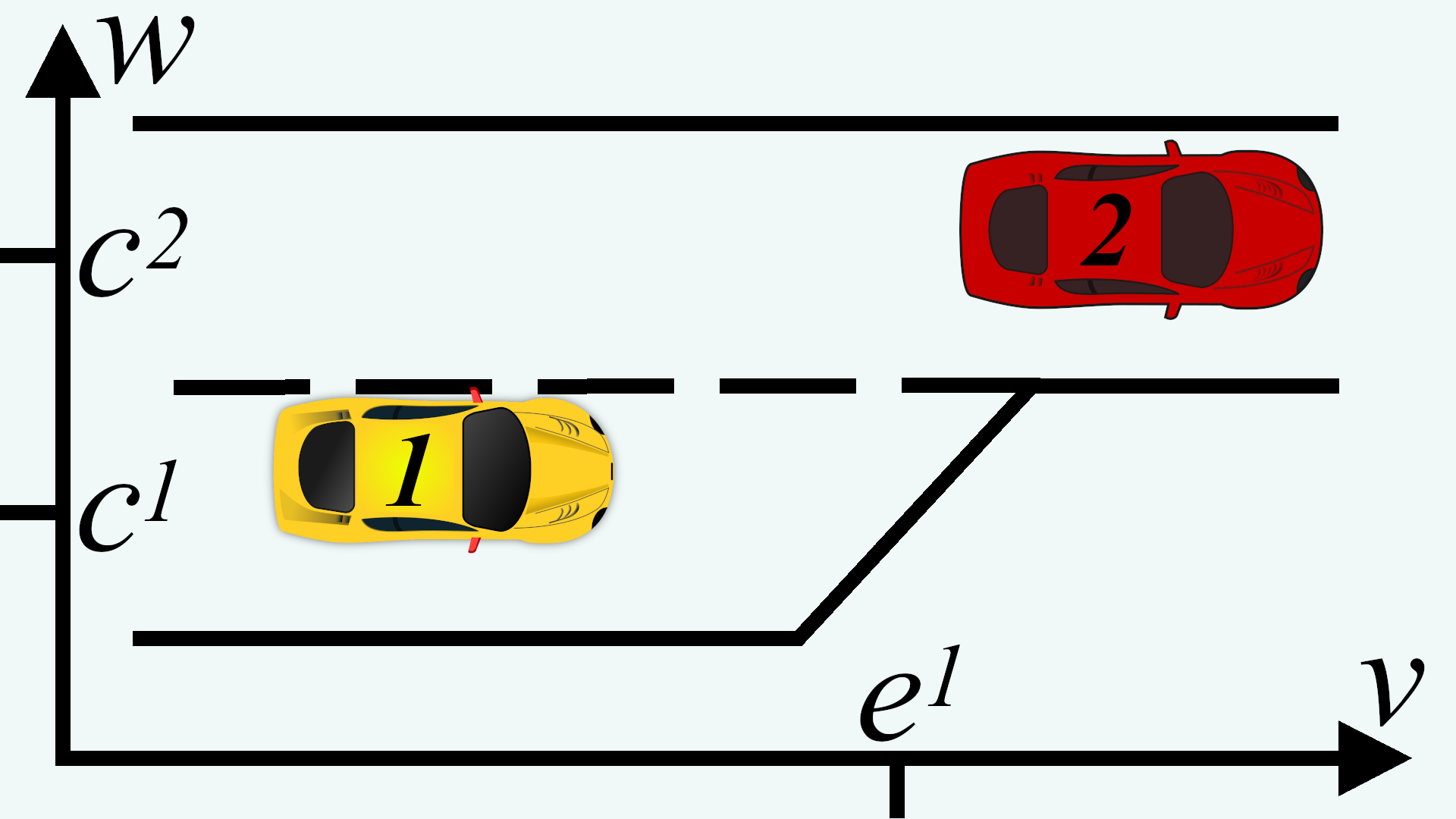
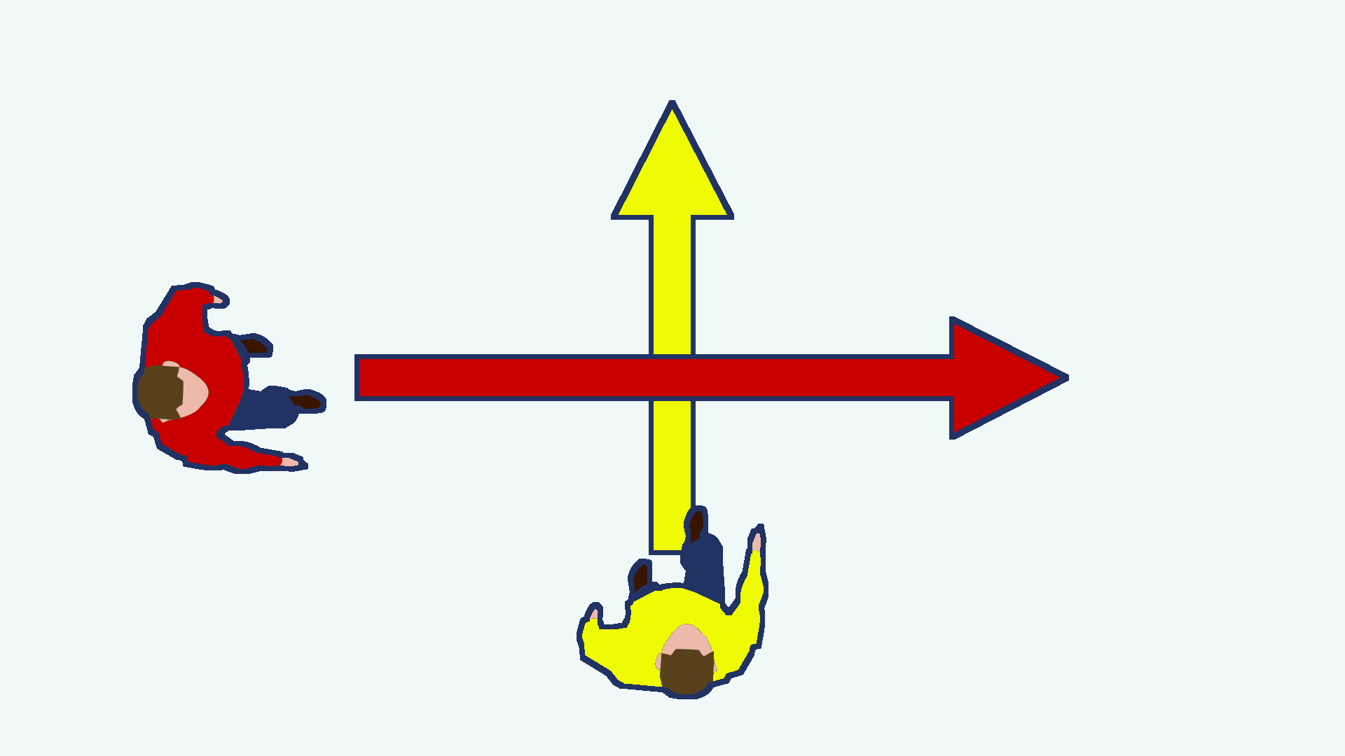
Figure 2: Left: Simple illustration of Scenario 1’s variables. Right: Illustration of simplistic pedestrian encounter scenario (Sec. C in the appendix).

Scenario 1 (Multi-lane driver interaction).

Setting: The set of possible individual states, denote it by $Y_{0}$, is of the form $[b,c]\times[d,e]$ – positions on a road section. There are $m$ parallel lanes (some of which may end), parallel to the x-axis. Agent $i$’s action $a^{i}\in A^{i}$ is given by the sequence of planar (i.e., 2-D) positions denoted $(v^{i}_{t},w^{i}_{t})\in Y_{0},t=0,\ldots,T$, but not allowing backward moves (and possibly other constraints). Define the states $y^{i}_{t}:=((v^{i}_{t},w^{i}_{t}),(v^{i}_{t-1},w^{i}_{t-1}),(v^{i}_{t-2},w^{i}_{t-2}))$. And let $y^{i}$ be the linear interpolation. Game: Let, for $t=0,\ldots,T$, the stage utilities of agent $i$ in the game $\Gamma_{\theta}$ be the following sum of terms for distance between agents, distance to center of lane, desired velocities, acceleration penalty, and end of lane overshooting penalty, respectively:

$$u^{i,\theta}_{t}(y^{i}_{t})=-\theta^{\text{dist}}\sum\frac{1}{|v^{j^{\prime}}_{t}-v^{j}_{t}|{+}\zeta}-\theta^{\text{cen},i}_{t}(w^{i}_{t}{-}c^{i}_{t})^{2}$$ (2a)

$$-\theta^{\text{vel},i}_{t}(\delta v^{i}_{t}-\theta^{\text{v},i})^{2}-\theta^{\text{velw},i}(\delta w^{i}_{t})^{2}-\theta^{\text{acc},i}(\delta^{2}v^{i}_{t})^{2}$$ (2b)

$$-\theta^{\text{end},i}\max(0,v_{t}-e^{i}_{t}),$$ (2c)

where the sum ranges over all $(j,j^{\prime})$ such that driver $j$ is right before $j^{\prime}$ on the same lane; $\zeta>0$ is a constant, $c^{i}_{t}$ is the respective center of the lane, $\delta v^{i}_{t}$ means velocity along lane, $\delta w^{i}_{t}$ means lateral velocity, $\delta^{2}v^{i}_{t}$ means acceleration (vector), $e^{i}_{t}$ is the end of $i$’s lane, if it ends, otherwise $-\infty$; furthermore, $\mu$ is the counting measure on $\{0,\ldots,T\}$ (i.e., discrete). and $\theta{=}(\theta^{\text{dist}},\theta^{\text{cen},i}_{[0:T]},\theta^{\text{vel},i}_{[0:T]},\theta^{\text{v},i},\theta^{\text{velw},i},\theta^{\text{acc},i},\theta^{\text{end},i})_{i\in I}$. Action subspaces: Consider the following equivalence relation on the trajectory space $Y$: two joint trajectories $y,y^{\prime}\in Y$ are equivalent if at each time point $t$, (1) each agent $i$ is on the same lane in $y$ as in $y^{\prime}$, and (2) within each lane, the order of the agents (along the driving direction) is the same in $y$ as in $y^{\prime}$. Now let the subspace collection $(\tilde{A}_{k})_{k\in K}$ be obtained by taking the (closures of the) resulting equivalence classes.

Proposition 1 (Scenario 1’s suitability).

Scenario 1 satisfies Assumption 1. So, in particular, Thm. 1’s implications on the induced implicit layer hold true.

Our general approach (Sec. 3) in principle is also applicable to various other multiagent trajectory settings, such as pedestrian interaction, relevant for mobile robots. We analyze a simplistic such scenario in Sec. C in the appendix, see Fig. 2 (right) for a foretaste.

5 Experiments

We evaluate our approach on (1) an observational prediction task on two real-world data sets (Sec. 5.1), as well as (2) a simple decision-making transfer task (Sec. 5.2).

5.1 Prediction Task on Highway Merging Scenarios in Two Real-World Data Set

2.5 Data set	Metric	TGL (ours)	TGL-D (ours)	CS-LSTM	MFP
highD (Krajewski et al. 2018)	MAE	3.6	2.9	5.0	5.2
	RMSE	4.9	3.7	6.8	7.1
HEE (our new data set; Sec. 5.1)	MAE	3.7	3.2	3.6	3.7
	RMSE	4.7	4.1	4.3	4.8
2.5

Table 1: Prediction task: Our method(s) vs. state-of-the-art (CS-LSTM (Deo and Trivedi 2018), MFP (Tang and Salakhutdinov 2019)) for a prediction task on merging scenarios in two real-world highway data sets, averaged over a 7s prediction horizon.

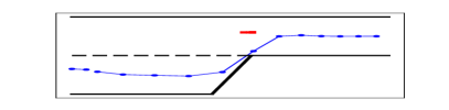
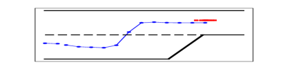
Figure 3: Decision-making transfer task: Solution trajectorie(s) that the (partially learned) game implies for the self-driving car’s decision-making task (each circle/square corresponds to one time step). Left: First local NE: the self-driving car (red) does a full emergency break and the other (blue) merges before it. Right: Second local NE: the other merges after it, both slow down.

We consider a highway merging interaction scenario with two cars similar as sketched in Fig. 1. This is considered a challenging scenario for autonomous driving.

Implementation details for our method for these merging scenario.

We use the following generic implementation of our general approach (Sec. 3), with concrete setting, game and action subspaces from Scenario 1 (with $n=2$), referring to it as TGL (trajectory game learner): We use validation-based early stopping. We combine equilibrium refinement and weighting net into one module, consisting of two nets that predict the weights $({\prescript{k}{}{\hat{q}}})_{k\in\tilde{K}}$ on the combination of (1) merging order (before/after) probabilities via a cross-entropy loss (2 hidden layers: $1\times 16$, $1\times 4$ neurons; dropout 0.6), and (2) Gaussian distribution over merging time point (discretized and truncated, thus the support inducing a refinement; 2 hidden layers: $1\times 64$, $1\times 32$ neurons; dropout 0.6), given $x$. For the preference revelation net we use a feed forward net (two hidden layers: $1\times 16$, $1\times 24$ neurons). As training loss we use mean absolute error (MAE; see also evaluation details below).

Besides this generic instantiation, we also consider a version of it, termed TGL-D: Instead of predicting the desired velocity $\theta^{\text{v},i}$ itself, the preference revelation net predicts the difference to the past velocity, and then squashes this into a sensible range using a sigmoid. (This can be seen as encoding a bit of additional prior knowledge which may not always be easy to specify and depend on the situation.) For further details, see Sec. D in the appendix. Code is available at: https://github.com/boschresearch/trajectory_games_learning.

Baselines.

As baselines we use the state-of-the-art data-driven methods “convolutional social pooling” – specifically: CS-LSTM (Deo and Trivedi 2018) – and “Multiple Futures Prediction” (MFP) (Tang and Salakhutdinov 2019). Evaluation. We use four-fold cross validation (splitting the data into 4 $\times$ 75% train and 25% validation). As metrics, we use rooted mean squared error (RMSE) and MAE (in meters) between predicted future trajectory $\hat{y}$ and truth $y$, averaged over a 7s horizon, with prediction step size of 0.2s, applying this to the most likely mode given by our method.

Data sets (one new one) and filtering:

1st data set: We use the “highD” data set (Krajewski et al. 2018), which consists of car trajectories recorded by drones over several highway sections. It is increasingly used for benchmarking (Rudenko et al. 2019; Zhang et al. 2020). From this data set, we use the recordings done over a section with an on-ramp.

2nd data set: We publish a new data set with this paper, termed HEE (Highway Eagle Eye). It consists of $\sim$12000 individual car trajectories ($\sim$4h), recorded by drones over a highway section (length $\sim$600m) with an entry lane. The link to the data set and further details are in Sec. D.2 in the appendix. Keep in mind that this data set can be useful for studies like ours, but some aspects of it may be noisy, so it is only meant for such experimental purposes.

Selection of merging scenes in both data sets: We filter for all joint trajectories of two cars where one is merging from the on-ramp, one is on the rightmost highway lane, and all other cars are far enough to not interact with these two. This leaves 25 trajectories of highD and 23 of our new data set.

Results.

The results are in Table 1 (with more details in Sec. D in the appendix). Our generic method TGL outperforms CS-LSTM and MFP on highD. And our slightly more hand-crafted method TGL-D outperforms them on both data set. Keep in mind that the data sets are small. So, while the results do indicate the practicality of our method in this small-sample regime, their significance is comparably limited.

5.2 Simple Decision-Making Transfer Task in Simulation

As discussed in Sec. 3.2 the game $\Gamma_{\theta}$ – once $\theta$ is given, e.g., by our learned preference revelation net – naturally transfers to decision-making tasks in situations with multiple strategic agents (something which predictive methods like the above CS-LSTM usually cannot do). To test and illustrate its ability for this, we consider a simple scenario: Take the above two-car highway on-ramp situation (Sec. 5.1, Scenario 1), but assume that the car on the highway lane is a self-driving car. Assume it has a technical failure roughly at the height of the on-ramp’s end, and it should do an emergency break (i.e., desired velocity $\theta^{\text{v},i}$ in (2) is set to 0) while at the same time ensuring that the other car coming from the on-ramp will not crash into it. Which trajectory should it choose? Result. Fed with this situation, our game solver suggests two possible solutions – two local NE, see Fig. 3: (1) the self-driving car completely stops and the on-ramp car will merge in front of it, accepting to touch the on-ramp’s end; (2) the self-driving car moves slowly, but at a non-zero speed, with the other car right behind it (keeping a rational distance). While a toy scenario, we feel that these are sensible solutions. Note that, Additionally, this shows that we (similar to IRL) have a strong ability to reasonably generalize out of sample, since a fully braking vehicle is actually not in the data.

6 Conclusion

For modeling of realistic continuous multiagent trajectories, in this work we proposed an end-to-end trainable model class that hybridizes neural nets with game-theoretic reasoning. We accompanied it with theoretical guarantees as well as an empirical demonstration of its practicality, on real-world highway data. We consider this as one step towards machine learning methods for this task that are more interpretable, verifiable and transferable to decision making. This is particularly relevant for safety-critical domains that involve interaction with humans. A major challenge is to make game-theoretic concepts tractable for such settings, and we were only partially able to address this. Specifically, potential for future work lies in relaxing subspace-wise concavity, common-coupled games and related assumptions we made.

Appendix

Appendix A Proofs and remarks

A.1 Lemma 1

Let us first restate the result.

Lemma 1.

If $\Gamma_{\theta}$ is a common-coupled game, then it is a potential game with the following potential function, where, as usual, $y=r(a)$:

$$\psi(a,\theta)=\int_{0}^{T}u^{\text{com},\theta}_{t}(y_{t})+\sum_{i\in I}u^{\text{own},i,\theta}_{t}(y^{i}_{t})d\mu(t).$$

Proof of Lemma 1.

Recall that based on the definition of a common-coupled game we have have for the stage-wise utility for all $i$ and $t$,

$$u^{i,\theta}_{t}(y_{t}) =u^{\text{com},\theta}_{t}(y_{t})+u^{\text{own},i,\theta}_{t}(y^{i}_{t})+u^{\text{oth},i,\theta}_{t}(y^{-i}_{t}).$$ (3)

Intuitively, the statement directly follows because taking the “derivative”of $i$’s utility above w.r.t. $y^{i}$ will just leave the derivative of the common term and $i$’s own term, because the other is constant in $y^{i}$. And the same happens for $\psi$.

Formally, observe that for all $i$ and $t$,

$$u^{i,\theta}_{t}((y^{i\prime}_{t},y^{-i}_{t}))-u^{i,\theta}_{t}((y^{i}_{t},y^{-i}_{t}))$$

$$=u^{\text{com},\theta}_{t}((y^{i\prime}_{t},y^{-i}_{t}))-u^{\text{com},\theta}_{t}((y^{i}_{t},y^{-i}_{t}))$$

$$+u^{\text{own},i,\theta}_{t}(y^{i\prime}_{t})-u^{\text{own},i,\theta}_{t}(y^{i}_{t})+0$$

$$=u^{\text{com},\theta}_{t}((y^{i\prime}_{t},y^{-i}_{t}))-u^{\text{com},\theta}_{t}((y^{i}_{t},y^{-i}_{t}))$$

$$+u^{\text{own},i,\theta}_{t}(y^{i\prime}_{t})-u^{\text{own},i,\theta}_{t}(y^{i}_{t})+\sum_{j\in I\setminus i}u^{\text{own},j,\theta}_{t}(y^{j}_{t})-\sum_{j\in I\setminus i}u^{\text{own},j,\theta}_{t}(y^{j}_{t}).$$

Integrating w.r.t. $t$ and using the linearity of the integral completes the proof. ∎

A.2 Theorem 1

Let us first restate the result.

Theorem 1 (Game-induced differentiable implicit layer).

Let Assumption 1 hold true. Then, for each $k\in K$, there is a continuous mapping $g_{k}:\Theta\to\tilde{A}_{k}$, such that for any $\theta\in\Theta$, if $g_{k}(\theta)$ lies in the interior of $\tilde{A}_{k}$, then

• $g_{k}(\theta)$ is a local NE of $\Gamma_{\theta}$,

• $g_{k}(\theta)$ is given by the unique argmax of $\psi(\theta,\cdot)$ on $\tilde{A}_{k}$, with $\psi$ the game’s potential function (Lem. 1),

• $g_{k}$ is continuously differentiable in $\theta$ with gradient

  $$J_{\theta}g_{k}(\theta)=-\left(H_{a}\psi(\theta,a)\right)^{-1}J_{\theta}\nabla_{a}\psi(\theta,a),$$

  whenever $\psi$ is twice continuously differentiable on an open set containing $(\theta,a)$, for $a=g_{k}(\theta)$, where $\nabla,J$ and $H$ denote gradient, Jacobian and Hessian, respectively.

Proof of Theorem 1.

Gradient etc.

Based on Lemma 1, the potential function $\psi$ exists. Let $k\in K$ be arbitrary but fixed. Let $g_{k}$ be the function that maps each $\theta$ to the corresponding unique maximum of $\psi(\theta,\cdot)$ on $\tilde{A}_{k}$ (exists and is unique by the assumption of strict concavity and convexity and compactness of the $\tilde{A}_{k}$). From the definition of the potential function and the local Nash equilibrium (NE), it follows directly that a maximum of the potential function is a local NE of the game.

To apply the implicit function theorem, let us consider the point $(\theta,g_{k}(\theta))$. If the minimum $g_{k}(\theta)$ lies in the interior of $\tilde{A}_{k}$, and $\psi$ is continuously differentiable on an open set containing $(\theta,g_{k}(\theta))$, then we have $\nabla_{a}\psi(\theta,a)|_{(\theta,a)=(\theta,g_{k}(\theta))}=0$ and furthermore, by assumption of strict concavity, $J_{a}\nabla_{a}\psi(\theta,a)|_{(\theta,a)=(\theta,g_{k}(\theta))}$ non-singular. Then the implicit function theorem implies that there is a an open set $O$ containing $(\theta,g_{k}(\theta))$, and a unique continuously differentiable function $f:O\to\tilde{A}_{k}$, such that $\nabla_{a}\psi(\theta^{\prime},f(\theta^{\prime}))=0$ for $\theta^{\prime}\in O$, with gradient

$$J_{\theta}f(\theta)=-\left(J_{a}\nabla_{a}\psi(\theta,a)\right)^{-1}J_{\theta}\nabla_{a}\psi(\theta,a)=-\left(H_{a}\psi(\theta,a)\right)^{-1}J_{\theta}\nabla_{a}\psi(\theta,a).$$ (4)

Now on $O$, $f$ and $g_{k}$ coincide since $f$ is uniquely determined (specifically, based on the implicit function theorem, locally, the graph of $f$ coincides with the solution set of $\nabla_{a}\psi(\cdot,\cdot)=0$, and if $f,g_{k}$ would differ in at least one point $\theta^{\prime}$, then there would be a solution $(\theta^{\prime},g_{k}(\theta^{\prime}))$ outside the solution set – a contradiction). Therefore $g_{k}$ is also continuously differentiable on $O$ with gradient

$$J_{\theta}g_{k}(\theta)=J_{\theta}f(\theta).$$ (5)

We can do this for every $\theta$, which completes the proof.

Continuity.

Since $\psi$ is continuous, $\tilde{A}_{k}$ is compact, and the maxima are unique, the maximum theorem implies that the mapping $g_{k}$ is in fact continuous (hemicontinuity reduces to continuity when the correspondence is in fact a function).

∎

A.3 Lemma 2 with remark on zero gradient

Let us first restate the result.

Lemma 2.

Let Assumption 1 hold true and additionally assume $\psi$ to be continuously differentiable on (a neighborhood of) $\Theta\times\tilde{A}_{k},k\in K$. If $a=g_{k}(\theta)$ lies on (exactly) one constraining affine hyperplane of $\tilde{A}_{k}$, defined by orthogonal vector $v$, with multiplier $\lambda$ and optimum $\lambda^{*}>0$ of $\psi(\theta,a)$’s Lagrangian (details in the proof), then $J_{\theta}g_{k}(\theta)=\left[-\left(\begin{array}[]{cc}H_{a}\psi(\theta,a)&v\\ \lambda^{*}v^{T}&0\\ \end{array}\right)^{-1}\left(\begin{array}[]{c}J_{\theta}\nabla_{a}\psi(\theta,a)\\ 0\end{array}\right)\right]_{1:(n\cdot{d_{A}})\times 1:(n\cdot{d_{A}})}$.

Remark on zero gradient.

Note that under the conditions of this lemma, i.e., when $g_{k}(\theta)$ lies at the boundary, then the above gradient $J_{\theta}g_{k}(\theta)$ in fact often becomes zero, which can be a problem for paramter fitting. So the above result is only meant as a first step.

Proof of Lemma 2.

Let $\tilde{A}_{k}$ be defined by the inequality constraints $v_{m}^{T}a\leq b,m=1,\ldots,M$. Consider the Lagrangian

$$\Lambda(\theta,a,\lambda_{1},\ldots,\lambda_{M})=\psi(\theta,a)+\sum_{m}\lambda_{m}(v_{m}^{T}a-b).$$

Then the Karush-Kuhn-Tucker optimality conditions (Boyd and Vandenberghe 2004) (note that we assumed differentiability of $\psi$ on a a neighborhood of $\Theta\times\tilde{A}_{k},k\in K$) include the following equations:

$$\nabla_{a}\Lambda(\theta,a,\lambda_{1},\ldots,\lambda_{M}) =0,$$ (6a)

$$\lambda_{m}(v_{m}^{T}a-b) =0,\ m=1,\ldots,M.$$ (6b)

Now let $a^{*}=g_{k}(\theta)$ and let $\lambda^{*}_{1},\ldots,\lambda^{*}_{M}$ be the (optimal) duals for $a^{*}$. And assume that $a^{*}$ lies on exactly one bounding (affine) hyperplane. W.l.o.g. let this hyperplane correspond to $v_{1},\lambda^{*}_{1}$. Also recall that $g_{k}$ is continuous (as in Theorem 1). Therefore, in a neighborhood of $\theta$, the corresponding optimum will not lie within any of the other boundaries. So in this neighborhood of $\theta$, all corresponding optimal duals will be zero (inactive) except for the assumed one.

Therefore, given a $\theta^{\prime}$ from the mentioned neighborhood of $\theta$, we have that $a,v_{1}$ satisfy the optimality conditions in (6) (for some remaining duals) iff they satisfy the reduced conditions

$$\nabla_{a}\Lambda(\theta^{\prime},a,\lambda_{1},\lambda,0,\ldots,0) =0,$$ (7a)

$$\lambda_{1}(v_{1}^{T}a-b) =0.$$ (7b)

For succinctness, in what follows we write $\lambda$ instead of $\lambda_{1}$, i.e., drop the subscript. Let

$$h(\theta^{\prime},a,\lambda) :=(\nabla_{a}\Lambda(\theta^{\prime},a,\lambda,0,\ldots,0),\lambda(v^{T}a-b))$$

$$=(\nabla_{a}\psi(\theta^{\prime},a)+\nabla_{a}\lambda(v^{T}a-b),\lambda(v^{T}a-b))$$

$$=(\nabla_{a}\psi(\theta^{\prime},a)+\lambda v^{T},\lambda(v^{T}a-b))$$

So the conditions in (7) are

$$h(\theta^{\prime},a,\lambda)=0.$$ (8)

Similar as in Theorem 1, around the point $\theta,a^{*},\lambda^{*}$, $g_{k}$ satisfies (8) (for some $\lambda$’s). So we can apply the implicit function theorem to get its gradient.

We have

$$J_{(\theta,a,\lambda)}h(\theta,a,\lambda)$$

$$=\left(\begin{array}[]{ccc}J_{\theta}\psi(\theta,a)&H_{a}\psi(\theta,a)&v^{T}\\ 0&\lambda v^{T}&v^{T}a-b\\ \end{array}\right).$$

Note that

$$\left(\begin{array}[]{cc}H_{a}\psi(\theta,a^{*})&v^{T}\\ \lambda^{*}v^{T}&v^{T}a^{*}-b\\ \end{array}\right)=\left(\begin{array}[]{cc}H_{a}\psi(\theta,a^{*})&v^{T}\\ \lambda^{*}v^{T}&0\\ \end{array}\right)$$

is invertible, since

$$\det\left(\left(\begin{array}[]{cc}H_{a}\psi(\theta,a^{*})&v^{T}\\ \lambda^{*}v^{T}&0\\ \end{array}\right)\right)=\det(H_{a}\psi(\theta,a^{*}))\det(-\lambda^{*}v^{T}(H_{a}\psi(\theta,a^{*}))^{-1}v)$$

and both factors are non-zero since $H_{a}\psi(\theta,a^{*})$ is positive definite and $\lambda^{*},v$ are non-zero.

Therefore, the implicit function theorem is applicable to the equation, and we get as gradient

$$J_{\theta}g_{k}(\theta)=-\left(\begin{array}[]{cc}H_{a}\psi(\theta,a^{*})&v^{T}\\ \lambda^{*}v^{T}&0\\ \end{array}\right)^{-1}\left(\begin{array}[]{c}J_{\theta}\psi(\theta,a^{*})\\ 0\end{array}\right)$$

∎

A.4 Proposition 1

Let us first restate the result.

Proposition 1 (Scenario 1’s suitability).

Scenario 1 satisfies Assumption 1. So, in particular, Thm. 1’s implications on the induced implicit layer hold true.

Proof of Proposition 1.

Common-coupled game.

It is directly clear from the form of the utilities in Scenario 1, that this forms a common-coupled game.

Strict concavity of the potential function.

Observe that, for each $i$, within any one subspace $\tilde{A}_{k}$, for each $t$,

• $i$ does not changes lane, so $c_{t},e_{t}$ are simple constants.

• For each lane, there is a fixed set of agents. Consider the set $S$ of pairs $(j,j^{\prime})$ of agents that are on this lane and $j$ is right before $j^{\prime}$. This ordering (and thus $S$) is invariant within $\tilde{A}_{k}$. Therefore the agent distance term can be rewritten like

  $$\theta^{\text{dist}}\sum_{\text{$j$ right before $j^{\prime}$ on same lane}}\frac{1}{|v^{j}_{t}-v^{j^{\prime}}_{t}|+\zeta}$$ (9)

  $$=\theta^{\text{dist}}\sum_{{(j,j^{\prime})\in S}}\frac{1}{v^{j^{\prime}}_{t}-v^{j}_{t}+\zeta}$$ (10)

So all terms are concave (the other terms are obviously concave), therefore the overall potential function, which is just a sum of them, is concave.

Futhermore, note that the sum of all velocity and distance to lane center terms is a sum of functions such that for each component of the vector $a$ there is exactly one function of it, and only of it; and each function is strictly concave. This implies that the overall sum is strictly concave in the whole $a$. So the potential function is a sum of concave and a strictly concave term, meaning it is strictly concave.

NB: On the subspaces, the potential function is also differentiable.

Compactness and linearity of constraints.

Besides the constraints that define the compact complete action space $A$, which are obviously linear, the constraints that define the action subspaces $\tilde{A}_{k}$ are given by the intersection of constraints for each time point $t$ that are all of the form

• $w^{i}_{t}\geq\text{const.}$ or $w^{i}_{t}\leq\text{const.}$, or

• $v^{i}_{t}\leq v^{j}_{t}$,

so they are linear.

∎

Appendix B Further details on general architecture

Elaborating on Sec. 3.2: Alg. 1 describes TGL’s forward pass, in particular the parallel local NE search over the refined subspaces. Alg. 2 describes the training more formally, in particular the splitting into first training the equilibrium refinement net alone.

Input: past joint trajectory $x$

Output: modes ${\prescript{k}{}{\hat{y}}}$ and their probabilities ${\prescript{k}{}{\hat{q}}}$, $k\in\tilde{K}$, as prediction for future joint trajectory $y$

1 $\theta$ $=$ preference revelation net $(x)$ ;

2 $\tilde{K}$ $=$ equilibrium refinement net $(x)$;

// Implicit layer $g$:

3 foreach $k\in\tilde{K}$  do

       // Solve for local NE ${\prescript{k}{}{a^{*}}}$ in $\tilde{A}_{k}$:

4       ${\prescript{k}{}{a^{*}}}=g_{k}(\theta)=\arg\max_{a}\psi(\theta,a)$ s.t. ${a\in\tilde{A}_{k}}$;

5      

6$({\prescript{k}{}{\hat{y}}})_{k\in\tilde{K}}$ $=$ trajectory parametrization $r$ $(({\prescript{k}{}{a^{*}}})_{k\in\tilde{K}})$ ;

7 $({\prescript{k}{}{\hat{q}}})_{k\in\tilde{K}}$ $=$ eq. weighting net $(\theta,({\prescript{k}{}{a^{*}}})_{k\in\tilde{K}}),\ldots)$;

Algorithm 1 TGL – forward pass (sketch)

Input: set $S$ of training samples $(x^{\prime},y^{\prime}),(x^{\prime\prime},y^{\prime\prime}),\ldots$

// Train equilibrium refinement net:

1 Train the weights $w_{\text{er}}$ of the equilibrium refinement net on pairs $(x,k)$, where $k\in K$ is the index of the subspace the ground truth $y$ lies in, for $(x,y)\in S$ ;

// Train full architecture but with the equilibrium refinement net’s weights fixed:

2 Perform gradient-based training of the full architecture by training all its weights except for the equilibrium refinement net’s weights $w_{\text{er}}$ which are fixed to the one obtained by the training above. The forward pass is given by Alg. 1. To get gradients via back-propagation, for the implicit layer’s gradient use the formula given by Thm. 1 ;

Algorithm 2 TGL – training (sketch, in particular how to separate the equilibrium refinement net)

Appendix C Further example scenario: simple pedestrian encounter

Figure 4: Simplistic pedestrian encounter.

As indicated in the main text, let us now elaborate the second – pedestrian scenario – our general method applies to. When considering settings with characteristics such as continuous time, even if they still satisfy the conditions of our framework, to prove so can become arbitrarily complex. Here let us give a simplistic but verified second example with properties somewhat different from the first one: Consider two pedestrians who walk with constant velocity (this velocity is their respective action) along straight paths which are orthogonal and intersect such that they could bump into each other (Fig. 4). Formally:

Scenario 2 (Simple pedestrian encounter).

Setting: There are $n=2$ agents, the actions parameterize the trajectories via $y^{1}_{t}=(0,ta^{1}+z^{1})$, $y^{2}_{t}=(ta^{2}+z^{2},0)$ (for ease of notation, we put the intersection to the origin but translations are possible of course), the joint action space is $A=[\frac{z^{1}}{T},c]\times[\frac{z^{2}}{T},c]$, for constants $z^{1},z^{2}<0$ and $c>0$, (the lower bound on the action is to make sure they reach the intersection). Game: Let the final stage utility be given by the following sum of a distance penalty term and a desired velocity term

$$u^{i,\theta}_{T}(y^{i}_{T})=-h(\theta^{\text{dist}},a)\max_{t\in[0,T]}\frac{1}{\|y^{1}_{t}-y^{2}_{t}\|_{1}}$$ (11a)

$$-\theta^{\text{vel},i}(a^{i}-\theta^{\text{v},i})^{2}\text{ ($=-\infty$ if division by 0) },$$ (11b)

for some function $h$, $\theta^{\text{vel},i}>0$, and let $\mu$ be the Dirac measure on $T$. Action subspaces: Let the subspaces $(\tilde{A}_{k})_{k\in K}$ be given by (1) taking the two subspaces that satisfy $a_{k}\geq a_{2-k}+\varepsilon$, for $k=1,2$ respectively, and some small $\varepsilon>0$, i.e., split by which agent is faster, and (2) additionally split by which agent first reaches their paths’ intersection (altogether this yields two or three subspaces).

Proposition 2 (Scenario 2’s suitability and partial identifiability).

Assume Scenario 2 with $h(\theta^{\text{dist}},a)=\frac{1}{a_{k}}$, with $k$ the faster agent in $a$. Then Assumption 1 is satisfied. Furthermore, while the complete game parameter vector $\theta=(\theta^{\text{vel},1},\theta^{\text{v},1},\theta^{\text{vel},2},\theta^{\text{v},2},)$ is not identifiable in general, if $\theta^{\text{vel},i},i=1,2$ is constant, then $(\theta^{\text{v},1},\theta^{\text{v},2})$ is identifiable from $y$ on the pre-image of the interior of $\tilde{A}_{k}$, for any $k$.

C.1 Proof of Proposition 2

Proof of Proposition 2.

Remark on utility form.

Note that in Scenario 2 the stage-utility at time $T$ in its “distance term” uses a form of maximum operator that takes the whole trajectories as input. But according to our Definition 1, actually we allow the stage utility to only depend on respective current state. But this can be resolved by observing that the “distance term” can in fact be rewritten as a function of $(a^{1},a^{2})$, as we will see in Equation 17 below. And $(a^{1},a^{2})$ in turn is given by $(y^{T}_{1}-z^{1},y^{T}_{2}-z^{2})/T$, i.e., determined by $y^{T}$.

Common-coupled game.

It is directly clear from the form of the utilities in Scenario 2, that this forms a common-coupled game.

Strict concavity of the potential function.

Consider all subspaces $\tilde{A}_{k}$ where agent 1 is faster, i.e., $a_{1}>a_{2}$. Note that this can be one or two subspaces: if $y^{0}_{1}>y^{0}_{2}$, then it is one subspace, but otherwise it is two (namely, where 1 or 2 reaches the intersection first, respectively).

On any one of these subspaces, the following holds true:

Regarding the distance-based term, observe that

$$\text{arg min}_{t\in[0,T]}|t\cdot a^{1}+z^{1}|+|t\cdot a^{2}+z^{2}|=-\frac{z^{1}}{a^{1}}.$$ (12)

To see this, observe that the argmin is given by $t$ where agent 1 reaches the intersection, i.e, $t$ where $t\cdot a^{1}+z^{1}=0$, i.e., $t=-\frac{z^{1}}{a^{1}}$. (And this holds regardless of whether 1 or 2 first reaches the intersection.)

To see this in turn, first consider the case that agent $1$ first reaches the intersection. Then, before this $t$, both terms are bigger (both agents are further away from the origin), while at this $t$, the first term is 0, and after it the left term grows faster (because the agent is faster) than the right term decreases (until the right term hits $0$ as well and then also increases again).

Second, consider the case where agent $2$ first reaches the intersection (in case this happens at all – i.e., if 2 starts so much closer to the origin to make this possible). Then, before $2$ reaches the intersection: obviously both terms are bigger than when $2$ reaches the intersection. Between $2$ reaching the intersection and $1$ reaching the intersection: in this time span, the right term grows slower than the left term decreases, therefore the minimum (for this time span) happens when 1 reaches the intersection. Now after 1 has reached the intersection obviously both terms just grow.

Therefore,

$$u^{\text{com},\theta}_{T}(y_{[0,T]}) =-\frac{1}{a^{1}}\max_{t\in[0,T]}\frac{1}{\|(0,t\cdot a^{1}+z^{1})-(t\cdot a^{2}+z^{2},0)\|_{1}}$$ (13)

$$=-\frac{1}{a^{1}}\max_{t\in[0,T]}\frac{1}{|t\cdot a^{1}+z^{1}|+|t\cdot a^{2}+z^{2}|}$$ (14)

$$=-\frac{1}{a^{1}}\frac{1}{|-\frac{z^{1}}{a^{1}}\cdot a^{1}+z^{1}|+|-\frac{z^{1}}{a^{1}}\cdot a^{2}+z^{2}|}$$ (15)

$$=-\frac{1}{a^{1}}\frac{1}{|-\frac{z^{1}}{a^{1}}\cdot a^{2}+z^{2}|}$$ (16)

$$=-\frac{1}{|z^{2}a^{1}-z^{1}a^{2}|}$$ (17)

Keep in mind that for agent $i$, the time when it reaches the intersection is given by $t_{i}=-\frac{z^{i}}{a^{i}}$. Now, if, for the subspace under consideration, agent 1 first reaches the intersection, i.e., $-\frac{z^{1}}{a^{1}}>-\frac{z^{2}}{a^{2}}$, i.e., $\frac{z^{1}}{a^{1}}<\frac{z^{2}}{a^{2}}$, i.e., $z^{1}a^{2}<z^{2}a^{1}$. Then (17) becomes $-\frac{1}{z^{2}a^{1}-z^{1}a^{2}}$, which is obviously concave. Similarly for the case that agent 2 first reaches the intersection.

Regarding the velocity terms, obviously their sum is strictly concave.

So the sum of all terms is strictly concave.

Linearity and compactness of constraints.

The constraints are all of the form $a_{1}\geq a_{2}+\varepsilon$ or $z^{1}a^{2}<z^{2}a^{1}$, i.e., linear.

Identifiability.

Obviously the full $\theta$ cannot be identifiable because there are no (local) diffeomorphisms between spaces of differing dimension.

Keep in mind that the parametrization from $a$ to $y$ is injective, so we just need to show identifiability from $a$. That is, we have to show that $g_{k}$ is invertible on $g_{k}^{-1}(\mathit{int}(\bigcup_{k}\tilde{A}_{k}))$, where $\mathit{int}(\cdot)$ denotes the interior.

Since we fixed $\theta^{\text{vel},i},i=1,2$, consider them as constants, and for what follows, for simplicity let $\theta$ stand for $(\theta^{\text{v},1},\theta^{\text{v},2})$.

W.l.o.g. (the other cases work similarly) assume $\tilde{A}_{k}$ is the subspace where agent 1 is faster and first reaches the intersection, so the potential function becomes

$$\psi(\theta,a)=\frac{1}{z^{2}a^{1}-z^{1}a^{2}}-\theta^{\text{vel},1}(a^{1}-\theta^{\text{v},1})^{2}-\theta^{\text{vel},2}(a^{2}-\theta^{\text{v},2})^{2}.$$ (18)

Now let $a$ be such that $a=g_{k}(\theta)$ for some $\theta$. We have to show that there can only be one such $\theta$. To see this, note that $a$ is a local NE, and thus

$$0=\nabla_{a}\psi(\theta,a)=\left((-1)^{i-1}\frac{z^{3-i}}{(z^{2}a^{1}-z^{1}a^{2})^{2}}+2\theta^{\text{vel},i}a^{i}-2\theta^{\text{vel},i}\theta^{\text{v},i}\right)_{i=1,2}.$$ (19)

But this implies

$$\theta^{\text{v},i}=\frac{(-1)^{i-1}\frac{z^{3-i}}{(z^{2}a^{1}-z^{1}a^{2})^{2}}-2\theta^{\text{vel},i}a^{i}}{2\theta^{\text{vel},i}}.$$ (20)

∎

Appendix D Further details on experiments and implementation

Keep in mind that in the main text (Sec. 5), we already described two implementations/versions we propose as instantiations of our general method (Sec. 3.2) for the highway merging setting:

• TGL,

• TGL-D.

Here we present one further method:

• TGL-DP (also “TGL-P” for short) – building on TGL-D, we use the interpretable representation of the desired velocity parameter predicted by the preference revelation net, which we first validate, and then encode additional prior-knowledge based constraints (e.g., we clip maximum and minimum desired speed) – see Sec. D.1 for details.

Additionally, in this section we provide further details on the new data set (Sec. D.2) as well as more fine-grained empirical evaluations metrics (individual prediction time points) for all methods.

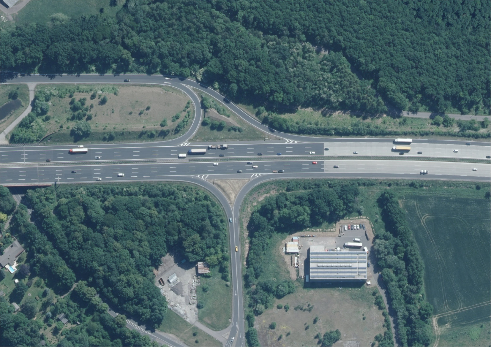
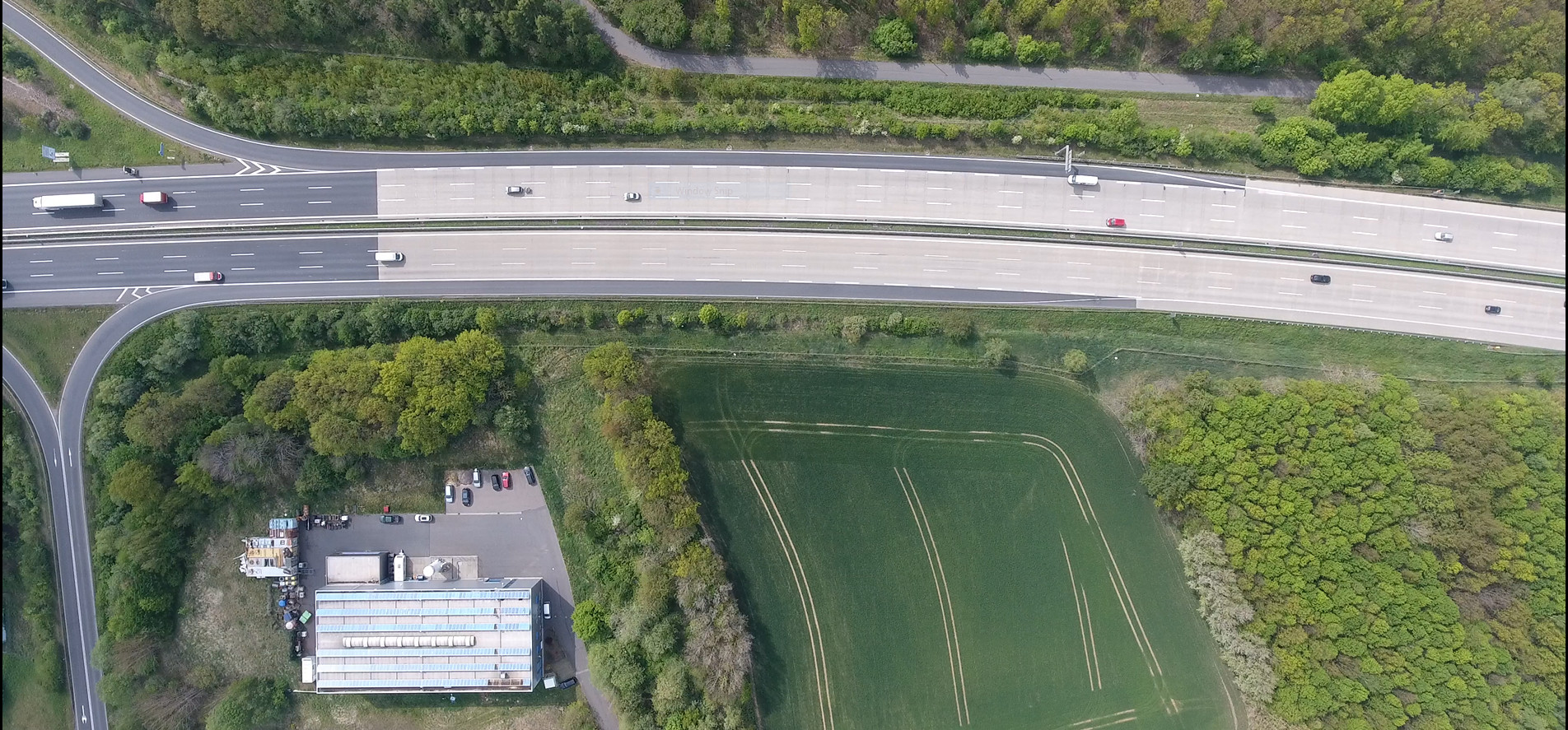
Figure 5: For the new highway data set , this is roughly the recorded highway section (only the lower lane, incl. exit/entry). Note that the recorded section is in fact slightly more to the right than the picture indicates.

Figure 6: This is a zoom-in on roughly the sub-part of the highway section in Fig. 6 that is relevant for the on-ramp merging trajectories used in the experiment.

D.1 More detailed description of TGL-DP

Input: old_vx_other,old_vx_merger // velocities along x-axis at the last step of the past trajectory $x$, where ‘‘merger’’ is the on-ramp car, and ‘‘other’’ is the highway car

 desired_vx_other,desired_vx_merger // output $\theta^{\text{v},2},\theta^{\text{v},1}$ of TGL’s original preference revelation net

 merger_in_front // most probable subspace given by equilibrium refinement/weighting net, whether merger merges before or after other

 big_change // parameter -- factor for allowed big change, for the experiment we used big_change = 1.2

 small_change // parameter -- factor for allowed small change, for the experiment we used small_change = 1.04

1

Output: new_vx_other,new_vx_merger // new desired velocity game parameters $\theta^{\text{v},2},\theta^{\text{v},1}$

2

3

4if merger_in_front == 0 then

       // if the highway vehicle is in front

       // clamp change of highway vehicle desired speed

5       new_vx_other = clamp(desired_vx_other, old_vx_other / small_change, old_vx_other*small_change)

       // only allow accelerating merger vehicle, but limit maximum speed change

6       new_vx_merger = clamp(desired_vx_merger, old_vx_merger, old_vx_merger*big_change)

7else

       // if the merger vehicle is in front

       // clamp desired merger velocity to make it coherent with driving in front of other

8       new_vx_merger = clamp(desired_vx_merger, min( old_vx_merger*big_change, old_vx_other/big_change), old_vx_merger*big_change)

       // also clamp the desired speed of the other, distinguishing between two cases:

9       if new_vx_merger $>$ old_vx_other then

10             new_vx_other = clamp(desired_vx_other, old_vx_other / small_change, old_vx_other*small_change)

11      else

12             new_vx_other = clamp(desired_vx_other, old_vx_other / big_change, old_vx_other)

13      

Algorithm 3 Part of preference revelation net of TGL-P that outputs the desired velocity game parameters $\theta^{\text{v},2},\theta^{\text{v},1}$ and differs compared to TGL

NB: on what follows, we refer to the method TGL-DP also simply by TGL-P:

Let us give further details on our method TGL-P, that was only briefly introduced in Appendix D. This method is the same as TGL-D described in Sec. 5.1 (building on Scenario 1), except that we modified the preference revelation net based on plausible reasoning and using parts of the equilibrium refinement/weighting net. Note that this is still a special case of our general architecture (Sec. 3.2) in the rigorous sense, just with a preference revelation net that incorporates a fair amount of additional reasoning and shares some structure with the equilibrium refinement net.

There are two reasons why we introduce TGL-P: First, the preference revelation net has to be trained together with the local game solver implicit layer. This means that training takes comparably long (we have an outer and an inner optimization loop, as described in Sec. 3.2). And one particular problem we experienced and have not fully solved yet, is that often the preference revelation net already starts overfitting while the game parameters that are learned “globally”, i.e., not inferred from the past trajectory by the preference revelation net, are not properly learned yet. Now TGL-P allows to demonstrate what we believe TGL itself can also achieve once the mentioned problems are overcome; in particular, it shows that the game model class ($\Gamma_{\theta}$) has a substantial capacity to resemble the future trajecories. Second, TGL-P shows how the intermediate representation $\theta$ can be inspected and high level knowledge/reasoning about agents’ preferences/utilities and behavior can be incoporated.

Specifically, TGL-P can be described as being the same as TGL, except that the part of preference revelation net of TGL that outputs $\theta^{\text{v},2},\theta^{\text{v},1}$ is replaced by Alg. 3 (on page 3). The function $clamp(\cdot)$ is, as usual, defined by

$$clamp(z,m,M)=\max(m,\min(z,M)),$$

i.e., clipping values to $m$ / $M$ if they are below / above. While the details of the algorithm may look complex, the main idea is simple: we clip the outputs of the preference revelation net if they are too far off compared to what one would expect given initial velocities and output of the equilibrium refinement/weighting net. The algorithm has two parameters $big\_change$ and $small\_change$, for which we used the values 1.2 and 1.04, respectively, in the experiment.

Note that, while in general, the equilibrium refinement/weighting net and the preference revelation net serve separate purposes, the reason why in TGL-P we share structure between them is mainly a pragmatic one: the equilibrium refinement/weighting net can be trained separately from the implicit layer and thus much faster – and we made the experience that it learns a reliable signal to predict the future (subspaces / selected equilibria).

D.2 Additional details and link for new highway data set HEE published alongside this paper

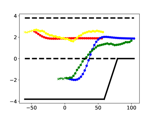
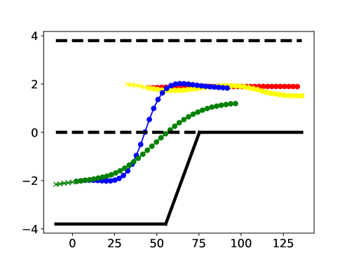
Figure 7: Example joint trajectories on highD data set (top) and our new highway data set (bottom). The ground truth future $y$ is green and yellow for on-ramp and highway car, respectively, with the past trajectory segment $x$ (at the very beginning) depicted by ’x’ markers. The prediction $\hat{y}$ (most likely mode) of our method TGL-P is in blue and red, respectively. Note that x- and y-axis are in meters; in particular, the x-axis is significantly squeezed.

One of the data sets we used in the experiment is a new one which we publish along this paper (introduced in Sec. 5.1). We refer to it as HEE (Highway Eagle Eye) data set. Here are the links relevant for the data set:

• Data set itself: https://github.com/boschresearch/hee_dataset.

• For example code of how to load/preprocess trajectories from the raw data set, please look at the code repository for this paper: https://github.com/boschresearch/trajectory_games_learning. Note that this repository also contains the precise filtered data set of two-player highway merge scenes that we used in the experiments.

Further remarks on HEE:

• The full recorded highway section in HEE is roughly as the lower lane (incl. exit/entry) in Fig. 6 (on page 6) (the recorded section is in fact slightly more to the right than the picture indicates). For the experiments we focused on merging scene trajectories, which roughly take place within the smaller highway section depicted in Fig. 6 (on page 6). Note that the images in Fig. 1 are a stylized (significantly squashed in the x-dimension) version of Fig. 6.

• Note that the recorded highway section in our data set – length $\sim 600$m – is longer compared to the one section with an on-ramp in the highD data set (Krajewski et al. 2018). But highD also contains other highway sections.

• As stated earlier, keep in mind that this HEE data set can be useful for studies like ours, but some aspects of it may be noisy, so it is only meant for experimental purposes.

D.3 More details on experimental results

2.5 Data set	Horizon	TGL (ours)	TGL-D (ours)	TGL-DP (ours)	CS-LSTM	MFP
highD (Krajewski et al. 2018)	1s	0.5	0.5	0.5	1.4	1.2
	2s	1.2	1.1	1.0	2.4	2.3
	3s	2.1	1.7	1.6	3.7	3.6
	4s	3.2	2.6	2.4	4.8	5.0
	5s	4.5	3.6	3.2	6.0	6.6
	6s	6.1	4.8	4.2	7.0	8.2
	7s	7.9	6.1	5.4	10.1	9.8
New data set (Sec. 5.1)	1s	0.8	0.7	0.8	0.8	0.8
	2s	1.5	1.4	1.5	1.6	1.6
	3s	2.4	2.2	2.3	2.3	2.4
	4s	3.5	3.1	3.0	3.3	3.6
	5s	4.6	4.0	3.9	4.4	4.6
	6s	5.9	4.9	4.7	5.3	5.8
	7s	7.3	5.9	5.6	7.2	7.1
2.5

Table 2: Mean absolute error (MAE) for all prediction horizons for all methods.

2.5 Data set	Horizon	TGL (ours)	TGL-D (ours)	TGL-DP (ours)	CS-LSTM	MFP
highD (Krajewski et al. 2018)	1s	0.6	0.5	0.5	1.8	1.6
	2s	1.4	1.2	1.2	3.2	3.0
	3s	2.7	2.1	2.0	5.0	4.8
	4s	4.3	3.2	3.0	6.3	6.8
	5s	6.1	4.5	4.2	7.7	9.0
	6s	8.4	6.1	5.7	9.1	11.2
	7s	11.0	8.0	7.6	14.5	13.6
New data set (Sec. 5.1)	1s	0.8	0.7	0.8	0.9	1.0
	2s	1.8	1.7	1.7	2.0	1.9
	3s	3.1	2.8	2.8	2.8	3.1
	4s	4.4	3.9	3.9	4.0	4.5
	5s	5.9	5.2	5.1	5.1	6.0
	6s	7.6	6.6	6.4	6.5	7.6
	7s	9.4	8.1	7.7	8.7	9.3
2.5

Table 3: Root mean square error (RMSE) for all prediction horizons for all methods.

In the main text we only gave results averaged over all prediction horizons. Here, Tables 3, 3 (on page 3) give the results – MAE and RMSE for all methods (including CS-LSTM (Deo and Trivedi 2018), MFP (Tang and Salakhutdinov 2019)) – for each prediction horizon individually, from 1s to 7s.

Additionally, in Fig. 7 (on page 7) we show example joint trajectories on highD data set and our new highway data set: the past trajectory $x$, the prediction $\hat{y}$ (most likely mode) of our method TGL-DP, and the ground truth future trajectory $y$. Note that the x-axis is significantly squeezed in these figures.

Appendix E Further related work

Regarding work that combines machine learning and game theory, noteworthy is also (Hartford, Wright, and Leyton-Brown 2016) who learn solution concepts, but not equilibrium refinement concepts. Generally, learning agent behavior, but in an active/experimental settings, is also extensively studied, e.g., in multiagent reinforcement learning (Shoham and Leyton-Brown 2008). Recently, also other related setting have been studied, e.g., where a computational assistant interacts with agents to learn their preferences and based on this support their coordination in the game-theoretic sense of equilibrium selection (Geiger et al. 2019).

Regarding imitation learning of agents’ interaction from observational data when there may be relevant unobserved confounders, there is also work based on causal models with a focus on identifiability analysis (Etesami and Geiger 2020; P. Haan 2018; Geiger, Hofmann, and Schölkopf 2016).

Beyond inverse reinforcement learning mentioned already in the introduction, our work is closely related to the general area of imitation learning (Osa et al. 2018).

Regarding probabilistic (multi-)agent trajectory prediction, on the machine learning side there are also recent methods using normalizing flows (Bhattacharyya et al. 2019, 2020).

Regarding implicit layers, the following work is also worth mentioning explicitly: Amos and Kolter (2017) take a (constrained) optimizer as implicit layer and derive the implicit layer’s gradient formula from the (Lagrangian/Karush-Kuhn-Tucker) optimality condition. Note that this is similar to one part of our Thm. 1, which, after the reduction to potential games, also derives the implicit layer’s gradient formula from an optimality condition. But our Thm. 1 contains additional elements in the sense of the precise preconditions to fit with the rest of our setting, the parallelization of solving for several local optima/equilibria, and the continuity implication for the $g_{k}$, which follows easily but which, so far, we have not seen in other work. Also note Amos et al. (2018) who differentiate through (single-agent) model predictive control (MPC) conditions. Worth mentioning are also Li et al. (2020), who also use implicit differentiation to learn about games.

Appendix F Remarks on rationality, local Nash equilibria, equilibrium selection, etc.

Let us make some high level remarks.

• As a remark on the (local) rationality principle in our model: We do not think that humans are perfectly instrumentally rational (i.e., strategic utility maximizers) in general, and in many multiagent trajectory settings bounded rationality and other phenomena may play an important role. Nonetheless, we believe that instrumental rationality is reasonably good approximation in many settings. And of course, game-theoretic rationality has the advantage that there is an elegant theory for it.

• In fact we use the local Nash equilibrium, which can also be seen as a bounded form of rationality. However, we feel that it can often be a better, more advanced approximation (to reality and/or rationality) than other concepts like level-k game theory (Stahl and Wilson 1995). In particular, we found it interesting that the local Nash equilibria can in fact correspond to intuitive modes of the joint trajectories, like which car goes first in Fig. 1. A reason for this may be that, while there may be one perfect solution (say a global Nash), due to errors and stochasticity of the environment the agents may be perturbed towards ending up at a state where a previously local Nash equilibrium may in fact now be a global Nash equilibrium.

• The problem of equilibrium selection mentioned in the main text may be seen as a form of incompleteness of game theory – it cannot always make a unique prediction (or prescription). Our equilibrium refinement and weighting nets can be seen as a data-driven approach to fill this incompleteness. An interesting question in this context is whether the missing information is actually contained in the preferences of the agents, or if there is additional (hidden) information required to find the unique solution/prediction.

• In some situations, it may be that knowledge of an (local-)equilibrium-separating partition may in fact tractably tell us the global Nash equilibrium (because if we know all local optima then we can also know the global optimum of a function). But this does not always seem to be the case for general common-coupled/potential games and, in particular, also because we do not require the equilibrium-separation to cover all possible equilibria.

References

- Alahi et al. (2016) Alahi, A.; Goel, K.; Ramanathan, V.; Robicquet, A.; Fei-Fei, L.; and Savarese, S. 2016. Social lstm: Human trajectory prediction in crowded spaces. In Proceedings of the IEEE conference on computer vision and pattern recognition, 961–971.
- Amos et al. (2018) Amos, B.; Jimenez, I.; Sacks, J.; Boots, B.; and Kolter, J. Z. 2018. Differentiable MPC for end-to-end planning and control. In Advances in Neural Information Processing Systems, 8289–8300.
- Amos and Kolter (2017) Amos, B.; and Kolter, J. Z. 2017. Optnet: Differentiable optimization as a layer in neural networks. In Proceedings of the 34th International Conference on Machine Learning-Volume 70, 136–145. JMLR. org.
- Bai, Kolter, and Koltun (2019) Bai, S.; Kolter, J. Z.; and Koltun, V. 2019. Deep equilibrium models. In Advances in Neural Information Processing Systems, 688–699.
- Bhattacharyya et al. (2019) Bhattacharyya, A.; Hanselmann, M.; Fritz, M.; Schiele, B.; and Straehle, C.-N. 2019. Conditional flow variational autoencoders for structured sequence prediction. NeurIPS Workshop on Machine Learning for Autonomous Driving .
- Bhattacharyya et al. (2020) Bhattacharyya, A.; Straehle, C.-N.; Fritz, M.; and Schiele, B. 2020. Haar Wavelet based Block Autoregressive Flows for Trajectories. German Conference on Pattern Recognition .
- Blaiotta (2019) Blaiotta, C. 2019. Learning generative socially aware models of pedestrian motion. IEEE Robotics and Automation Letters 4(4): 3433–3440.
- Boyd and Vandenberghe (2004) Boyd, S.; and Vandenberghe, L. 2004. Convex optimization. Cambridge university press.
- Camara et al. (2018) Camara, F.; Romano, R.; Markkula, G.; Madigan, R.; Merat, N.; and Fox, C. 2018. Empirical game theory of pedestrian interaction for autonomous vehicles. In Proceedings of Measuring Behavior 2018. Manchester Metropolitan University.
- Deo and Trivedi (2018) Deo, N.; and Trivedi, M. M. 2018. Convolutional social pooling for vehicle trajectory prediction. In Proceedings of the IEEE Conference on Computer Vision and Pattern Recognition Workshops, 1468–1476.
- El Ghaoui et al. (2019) El Ghaoui, L.; Gu, F.; Travacca, B.; and Askari, A. 2019. Implicit deep learning. arXiv preprint arXiv:1908.06315 .
- Etesami and Geiger (2020) Etesami, J.; and Geiger, P. 2020. Causal Transfer for Imitation Learning and Decision Making under Sensor‐shift. In Proceedings of the Thirty-Third AAAI Conference on Artificial Intelligence (AAAI).
- Etesami and Straehle (2020) Etesami, J.; and Straehle, C.-N. 2020. Non-cooperative Multi-agent Systems with Exploring Agents. arXiv preprint arXiv:2005.12360 .
- Fisac et al. (2019) Fisac, J. F.; Bronstein, E.; Stefansson, E.; Sadigh, D.; Sastry, S. S.; and Dragan, A. D. 2019. Hierarchical game-theoretic planning for autonomous vehicles. In 2019 International Conference on Robotics and Automation (ICRA), 9590–9596. IEEE.
- Fox et al. (2018) Fox, C.; Camara, F.; Markkula, G.; Romano, R.; Madigan, R.; Merat, N.; et al. 2018. When should the chicken cross the road?: Game theory for autonomous vehicle-human interactions .
- Geiger et al. (2019) Geiger, P.; Besserve, M.; Winkelmann, J.; Proissl, C.; and Schölkopf, B. 2019. Coordinating users of shared facilities based on data-driven assistants and game-theoretic analysis. In Proceedings of the 35th Conference on Uncertainty in Artificial Intelligence (UAI).
- Geiger, Hofmann, and Schölkopf (2016) Geiger, P.; Hofmann, K.; and Schölkopf, B. 2016. Experimental and causal view on information integration in autonomous agents. In Proceedings of the 6th International Workshop on Combinations of Intelligent Methods and Applications (CIMA 2016).
- Geiger and Straehle (2021) Geiger, P.; and Straehle, C.-N. 2021. Learning game-theoretic models of multiagent trajectories using implicit layers. In Proceedings of the Thirty-Fourth AAAI Conference on Artificial Intelligence (AAAI).
- Gupta et al. (2018) Gupta, A.; Johnson, J.; Fei-Fei, L.; Savarese, S.; and Alahi, A. 2018. Social GAN: Socially acceptable trajectories with generative adversarial networks. In Proceedings of the IEEE Conference on Computer Vision and Pattern Recognition, 2255–2264.
- Harsanyi, Selten et al. (1988) Harsanyi, J. C.; Selten, R.; et al. 1988. A general theory of equilibrium selection in games, volume 1. The MIT Press.
- Hartford, Wright, and Leyton-Brown (2016) Hartford, J. S.; Wright, J. R.; and Leyton-Brown, K. 2016. Deep learning for predicting human strategic behavior. In Advances in Neural Information Processing Systems, 2424–2432.
- Helbing and Molnar (1995) Helbing, D.; and Molnar, P. 1995. Social force model for pedestrian dynamics. Physical review E 51(5): 4282.
- Kang and Rakha (2017) Kang, K.; and Rakha, H. A. 2017. Game theoretical approach to model decision making for merging maneuvers at freeway on-ramps. Transportation Research Record 2623(1): 19–28.
- Kesting, Treiber, and Helbing (2007) Kesting, A.; Treiber, M.; and Helbing, D. 2007. General lane-changing model MOBIL for car-following models. Transportation Research Record 1999(1): 86–94.
- Kita (1999) Kita, H. 1999. A merging–giveway interaction model of cars in a merging section: a game theoretic analysis. Transportation Research Part A: Policy and Practice 33(3-4): 305–312.
- Kita, Tanimoto, and Fukuyama (2002) Kita, H.; Tanimoto, K.; and Fukuyama, K. 2002. A game theoretic analysis of merging-giveway interaction: a joint estimation model. Transportation and Traffic Theory in the 21st Century 503–518.
- Krajewski et al. (2018) Krajewski, R.; Bock, J.; Kloeker, L.; and Eckstein, L. 2018. The highD Dataset: A Drone Dataset of Naturalistic Vehicle Trajectories on German Highways for Validation of Highly Automated Driving Systems. In 2018 IEEE 21st International Conference on Intelligent Transportation Systems (ITSC).
- Kuderer et al. (2012) Kuderer, M.; Kretzschmar, H.; Sprunk, C.; and Burgard, W. 2012. Feature-based prediction of trajectories for socially compliant navigation. In Robotics: science and systems.
- Li et al. (2020) Li, J.; Yu, J.; Nie, Y.; and Wang, Z. 2020. End-to-end learning and intervention in games. Advances in Neural Information Processing Systems 33.
- Li et al. (2018) Li, N.; Kolmanovsky, I.; Girard, A.; and Yildiz, Y. 2018. Game theoretic modeling of vehicle interactions at unsignalized intersections and application to autonomous vehicle control. In 2018 Annual American Control Conference (ACC), 3215–3220. IEEE.
- Li and Liu (2018) Li, Y.; and Liu, H. 2018. Implementation of Stochastic Quasi-Newton’s Method in PyTorch. arXiv preprint arXiv:1805.02338 .
- Ling, Fang, and Kolter (2018) Ling, C. K.; Fang, F.; and Kolter, J. Z. 2018. What game are we playing? End-to-end learning in normal and extensive form games. In IJCAI-ECAI-18: The 27th International Joint Conference on Artificial Intelligence and the 23rd European Conference on Artificial Intelligence.
- Ling, Fang, and Kolter (2019) Ling, C. K.; Fang, F.; and Kolter, J. Z. 2019. Large scale learning of agent rationality in two-player zero-sum games. In Proceedings of the AAAI Conference on Artificial Intelligence, volume 33, 6104–6111.
- Liu et al. (2007) Liu, H. X.; Xin, W.; Adam, Z.; and Ban, J. 2007. A game theoretical approach for modelling merging and yielding behaviour at freeway on-ramp sections. Transportation and traffic theory 3: 197–211.
- Ma et al. (2017) Ma, W.-C.; Huang, D.-A.; Lee, N.; and Kitani, K. M. 2017. Forecasting interactive dynamics of pedestrians with fictitious play. In Proceedings of the IEEE Conference on Computer Vision and Pattern Recognition, 774–782.
- Monderer and Shapley (1996) Monderer, D.; and Shapley, L. S. 1996. Potential games. Games and economic behavior 14(1): 124–143.
- Osa et al. (2018) Osa, T.; Pajarinen, J.; Neumann, G.; Bagnell, J. A.; Abbeel, P.; and Peters, J. 2018. An algorithmic perspective on imitation learning. arXiv preprint arXiv:1811.06711 .
- Osborne and Rubinstein (1994) Osborne, M. J.; and Rubinstein, A. 1994. A course in game theory. MIT press.
- P. Haan (2018) P. Haan, D. Jayaraman, S. L. 2018. Causal Confusion in Imitation Learning. In NIPS Workshop.
- Peters et al. (2020) Peters, L.; Fridovich-Keil, D.; Tomlin, C. J.; and Sunberg, Z. N. 2020. Inference-Based Strategy Alignment for General-Sum Differential Games. arXiv preprint arXiv:2002.04354 .
- Ratliff, Burden, and Sastry (2013) Ratliff, L. J.; Burden, S. A.; and Sastry, S. S. 2013. Characterization and computation of local Nash equilibria in continuous games. In 2013 51st Annual Allerton Conference on Communication, Control, and Computing (Allerton), 917–924. IEEE.
- Ratliff, Burden, and Sastry (2016) Ratliff, L. J.; Burden, S. A.; and Sastry, S. S. 2016. On the characterization of local Nash equilibria in continuous games. IEEE Transactions on Automatic Control 61(8): 2301–2307.
- Reddy et al. (2012) Reddy, T. S.; Gopikrishna, V.; Zaruba, G.; and Huber, M. 2012. Inverse reinforcement learning for decentralized non-cooperative multiagent systems. In 2012 IEEE International Conference on Systems, Man, and Cybernetics (SMC), 1930–1935. IEEE.
- Robicquet et al. (2016) Robicquet, A.; Sadeghian, A.; Alahi, A.; and Savarese, S. 2016. Learning social etiquette: Human trajectory understanding in crowded scenes. In European conference on computer vision, 549–565. Springer.
- Rudenko et al. (2019) Rudenko, A.; Palmieri, L.; Herman, M.; Kitani, K. M.; Gavrila, D. M.; and Arras, K. O. 2019. Human motion trajectory prediction: A survey. arXiv preprint arXiv:1905.06113 .
- Salzmann et al. (2020) Salzmann, T.; Ivanovic, B.; Chakravarty, P.; and Pavone, M. 2020. Trajectron++: Multi-Agent Generative Trajectory Forecasting With Heterogeneous Data for Control. arXiv preprint arXiv:2001.03093 .
- Shoham and Leyton-Brown (2008) Shoham, Y.; and Leyton-Brown, K. 2008. Multiagent systems: Algorithmic, game-theoretic, and logical foundations. Cambridge University Press.
- Spica et al. (2018) Spica, R.; Falanga, D.; Cristofalo, E.; Montijano, E.; Scaramuzza, D.; and Schwager, M. 2018. A real-time game theoretic planner for autonomous two-player drone racing. arXiv preprint arXiv:1801.02302 .
- Stahl and Wilson (1995) Stahl, D. O.; and Wilson, P. W. 1995. On players’ models of other players: Theory and experimental evidence. Games and Economic Behavior 10(1): 218–254.
- Sun, Zhan, and Tomizuka (2018) Sun, L.; Zhan, W.; and Tomizuka, M. 2018. Probabilistic prediction of interactive driving behavior via hierarchical inverse reinforcement learning. In 2018 21st International Conference on Intelligent Transportation Systems (ITSC), 2111–2117. IEEE.
- Tang and Salakhutdinov (2019) Tang, C.; and Salakhutdinov, R. R. 2019. Multiple futures prediction. In Advances in Neural Information Processing Systems, 15398–15408.
- Tian et al. (2018) Tian, R.; Li, S.; Li, N.; Kolmanovsky, I.; Girard, A.; and Yildiz, Y. 2018. Adaptive game-theoretic decision making for autonomous vehicle control at roundabouts. In 2018 IEEE Conference on Decision and Control (CDC), 321–326. IEEE.
- Treiber, Hennecke, and Helbing (2000) Treiber, M.; Hennecke, A.; and Helbing, D. 2000. Congested traffic states in empirical observations and microscopic simulations. Physical review E 62(2): 1805.
- Wang and Klabjan (2018) Wang, X.; and Klabjan, D. 2018. Competitive multi-agent inverse reinforcement learning with sub-optimal demonstrations. arXiv preprint arXiv:1801.02124 .
- Wang et al. (2017) Wang, X.; Ma, S.; Goldfarb, D.; and Liu, W. 2017. Stochastic quasi-Newton methods for nonconvex stochastic optimization. SIAM Journal on Optimization 27(2): 927–956.
- Zazo et al. (2016) Zazo, S.; Macua, S. V.; Sánchez-Fernández, M.; and Zazo, J. 2016. Dynamic potential games with constraints: Fundamentals and applications in communications. IEEE Transactions on Signal Processing 64(14): 3806–3821.
- Zhang et al. (2020) Zhang, C.; Zhu, J.; Wang, W.; and Xi, J. 2020. Spatiotemporal Learning of Multivehicle Interaction Patterns in Lane-Change Scenarios. arXiv preprint arXiv:2003.00759 .
- Zhang et al. (2018) Zhang, Q.; Filev, D.; Tseng, H.; Szwabowski, S.; and Langari, R. 2018. Addressing Mandatory Lane Change Problem with Game Theoretic Model Predictive Control and Fuzzy Markov Chain. In 2018 Annual American Control Conference (ACC), 4764–4771. IEEE.
- Zhang et al. (2019) Zhang, X.; Zhang, K.; Miehling, E.; and Basar, T. 2019. Non-Cooperative Inverse Reinforcement Learning. In Advances in Neural Information Processing Systems, 9482–9493.