Simulation of plasma accelerators with the Particle-In-Cell method
Abstract
We present the standard electromagnetic Particle-in-Cell method, starting from the discrete approximation of derivatives on a uniform grid. The application to second-order, centered, finite-difference discretization of the equations of motion and of Maxwell’s equations is then described in one dimension, followed by two and three dimensions. Various algorithms are presented, for which we discuss the stability and accuracy, introducing and elucidating concepts like “numerical stochastic heating”, “CFL limit” and “numerical dispersion”. The coupling of the particles and field quantities via interpolation at various orders is detailed, together with its implication on energy and momentum conserving. Special topics of relevance to the modeling of plasma accelerators are discussed, such as moving window, optimal Lorentz boosted frame, the numerical Cherenkov instability and its mitigation. Examples of simulations of laser-driven and particle beam-driven accelerators are given, including with mesh refinement. We conclude with a discussion on high-performance computing and a brief outlook.
keywords:
Plasma-based acceleration; Computer simulations; Particle-in-cell method; high-performance-computing.1 Introduction
Computer simulations have had a profound impact on the design and understanding of past and present plasma acceleration experiments [1, 2, 3, 4], with accurate modeling of wake formation, electron self-trapping and acceleration requiring fully kinetic methods (usually Particle-In-Cell) using large computational resources (due to the wide range of space and time scales involved). Numerical modeling complements and guides the design and analysis of advanced accelerators, and can reduce development costs significantly. Despite the major recent experimental successes[5, 6, 7, 8, 9], the various advanced acceleration concepts need significant progress to fulfill their potential. To this end, large-scale simulations will continue to be a key component toward reaching a detailed understanding of the complex interrelated physics phenomena at play.
For such simulations, the most popular algorithm is the Particle-In-Cell (or PIC) technique, which represents electromagnetic fields on a grid and particles by a sample of macroparticles. These simulations are extremely computationally intensive, due to the need to resolve the evolution of a driver (laser or particle beam) and an accelerated beam into a structure that is orders of magnitude longer and wider than the accelerated beam. Hence, various techniques or reduced models have been developed to allow multidimensional simulations at manageable computational costs: quasistatic approximation [10, 11, 12, 13, 14], ponderomotive guiding center (PGC) models [11, 12, 14, 15, 16], simulation in an optimal Lorentz boosted frame [17, 18, 19, 20, 21, 22, 23, 24, 25, 26, 27, 28, 29], expanding the fields into a truncated series of azimuthal modes [30, 31, 32, 33, 34], fluid approximation [12, 35, 15] and scaled parameters [36, 37].
It is beyond the scope of the present report to review all or even most of the methods that have been developed. We will focus on the detailed presentation of the standard electromagnetic Particle-In-Cell method, as it is the most complete (as based on the first-principle Maxwell and particle motion equations) and versatile (as it can be applied to plasma and beam simulations way beyond plasma acceleration). For completeness, however, the quasistatic and ponderomotive guiding center models are given in Appendix A and B.
2 The electromagnetic Particle-In-Cell method
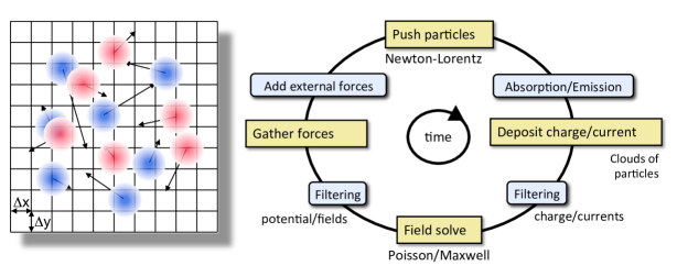
In the electromagnetic Particle-In-Cell method [38], the electromagnetic fields are solved on a grid, usually using Maxwell’s equations
| (1a) | |||||
| (1b) | |||||
| (1c) | |||||
| (1d) | |||||
given here in natural units (), where is time, and are the electric and magnetic field components, and and are the charge and current densities. The charged particles are advanced in time using the Newton-Lorentz equations of motion
| (2a) | ||||
| (2b) | ||||
where , , , and are respectively the mass, charge, position, velocity and relativistic factor of the particle given in natural units (). The charge and current densities are interpolated on the grid from the particles’ positions and velocities, while the electric and magnetic field components are interpolated from the grid to the particles’ positions for the velocity update.
If Eq. (1c) and Eq. (1d) are verified at a given time, they are also verified at any later time provided that Eq. (1a) and Eq. (1b) are verified together with the continuity equation . Hence Eq. (1c) and Eq. (1d) are often not solved explicitly in many codes.
2.1 Discretization of differential operations
A Taylor expansion of a function defined on a uniform grid of cell size writes
| (3a) | |||||
| (3b) | |||||
leading to the following first order approximations of the first derivatives
| (4a) | |||||
| (4b) | |||||
Substracting these two first-order approximations leads to the second-order centered finite-difference approximation
| (5) |
2.2 Particle push
2.2.1 Simple particle integrator
Neglecting relativity and magnetic fields, the motion equations
| (6a) | ||||
| (6b) | ||||
can be discretized - using the second-order centered finite-difference approximation - as
| (7a) | |||||
| (7b) | |||||
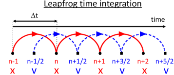
In this case, the quantities were staggered by half a time step, such that all finite-differences are centered and second-ordered. Such a scheme, which is represented graphically in Fig. 2, is called a “leapfrog” time integrator.
Stability
Let us consider the simple case of a linear force of the form , i.e. of a linear oscillator
| (8) |
The leapfrog discretization of this equation leads to
| (9) |
on which we perform a Von Neumann stability anaIysis. Inserting the ansatz into the last equation gives
| (10) |
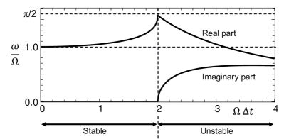
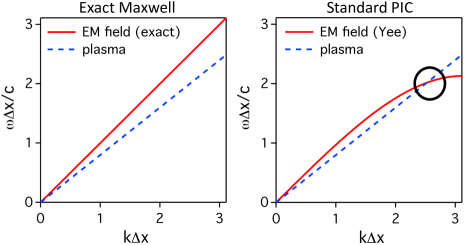
The solution to the last expression is plotted in Fig. 3. For , the scheme is stable. For the entire stable region, the frequency of the oscillations is higher than the real solution. The magnitude of the error on the frequency vanishes at and grows with . For , the scheme is unstable. The metastable solution at is called the Courant-Friedrichs-Lewy, or CFL, condition, which is one of the very common limits (but not the only one) on the time step that can be used in time-dependent computer simulations.
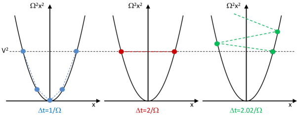
The origin of the CFL is easy to understand more intuitively by looking at the plot of the kinetic energy versus position for a harmonic oscillator initialized at rest with initial potential energy . The evolution of the kinetic energy is shown in Fig. 4 for a time step below the CFL (), a time step at the CFL () and a time step above the CFL ( ).
Numerical heating
Due to various approximations, it is common to introduce errors that can be interpreted as a random forces that give random velocity kicks . The average change in kinetic energy from these random kicks during one time step is given by
| (11a) | |||||
| (11b) | |||||
| (11c) | |||||
since . Hence, the average energy change after time steps is given by
| (12) |
This result shows that even if the numerical errors that affect the motion of the particles are random and average to zero, they will still result in a numerical “stochastic heating” that grows linearly in time and is proportional to the square of the time step. Since this type of error is typically unavoidable, it is important to always have it in mind when performing computer simulations.
2.2.2 Full particle integrator
The extension of the leapfrog integrator to the full set of relativistic Newton-Lorentz equations of motion is given by
| (13a) | ||||
| (13b) | ||||
Here again, all the quantities are centered properly to result in second-order centered finite-differences. This forces the velocity term that is involved in the magnetic rotation to be expressed as some average term to be determined. In order to close the system, must be expressed as a function of the other quantities. Some of the most popular implementations are presented below.
Boris pusher
Setting , the system of equations can be written as
| (15a) | |||||
| (15b) | |||||
| (15c) | |||||
Hence, the push is separated into one-half acceleration with the electric field, one rotation with the magnetic field and a second half acceleration with the electric field. The rotation is solved very efficiently by the Boris’ method using the following sequence:
| (16a) | ||||
| (16b) | ||||
where and where is given by .
The Boris implementation is second-order accurate, time-reversible and fast. Its implementation is very widespread and used in the vast majority of PIC codes.
Vay pusher
It was shown in [40] that the Boris formulation does not capture properly the case of complete - of near-complete - cancellation of the electric acceleration and magnetic rotation, compromising for example the modeling of ultra-relativistic charged particle beams.
An alternate velocity average was thus considered
| (17) |
which was shown to treat accurately the complete - of near-complete - cancellation of the electric acceleration and magnetic rotation.
The proposed velocity average leads to a system that is solvable analytically (see [40] for a detailed derivation), giving the following velocity update:
| (18a) | ||||
| (18b) | ||||
where , , , , and .
Higuera-Cary pusher
The solution proposed by Higuera and Cary [41] adopted the same form for the velocity average as Boris
| (19) |
but is now given by
| (20) |
Similarly to the Boris, pusher, we have
| (21a) | |||||
| (21b) | |||||
| (21c) | |||||
with , and where
| (22) |
with , , and .
Like the Boris pusher, the Higuera-Cary pusher is strictly “volume-preserving”, while the Vay pusher is not. Some comparison of the various pushers have been reported but there is not yet an exhaustive comparison of the three pushers for the modeling of plasma acceleration. This is an active area of research.
2.3 Field solve
Various methods are available for solving Maxwell’s equations on a grid, based on finite-differences, finite-volume, finite-element, spectral, or other discretization techniques that apply most commonly on single structured or unstructured meshes, and less commonly on multiblock multiresolution grid structures. In this chapter, we summarize the widespread second-order finite-difference time-domain (FDTD) algorithm, its extension to non-standard finite-differences, as well as the pseudo-spectral analytical time-domain (PSATD) algorithm.
2.3.1 Simple one-dimensional Leapfrog Maxwell solver
For simplicity, we consider first a one-dimensional wave equation without source term:
| (23a) | ||||
| (23b) | ||||
Similarly to the particle pusher, this system of equations can easily be discretized using Leapfrog space- and time-centered finite-differencing, giving
| (24a) | ||||
| (24b) | ||||
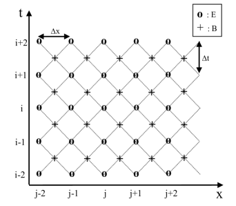
The electric and magnetic field components are defined on space-time grids that are staggered by half a space grid cell and half a time step, as depicted on Fig. 5.
Numerical accuracy and stability analyses
Performing a Von Neumann stability analysis, one makes the ansatz for waves propagating in the forward or backward direction. Applying to the terms in Eq. 24b at gives
| (25a) | ||||
| (25b) | ||||
| (25c) | ||||
| (25d) | ||||
Inserting into Eq. 24b and simplifying leads to
| (26) |
The phase and group velocities are thus given by
| (27a) | ||||
| (27b) | ||||
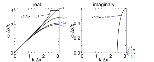
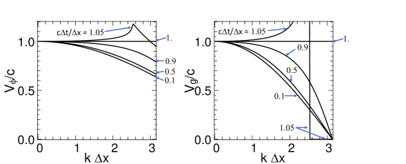
The values of , and are plotted in Fig. 6 as a function of , for various values of , leading to the following observations:
-
•
: the imaginary part of is null and the scheme is stable. The phase and group velocities are below the physical value , respectively as low as and at the Nyquist cutoff.
-
•
: the physical result is recovered, and all quantities are exact at all wavelengths. The time step is sometimes referred to as the “magical time step”.
-
•
: the imaginary part is positive, meaning that the solution is unstable and grows exponentially in time.
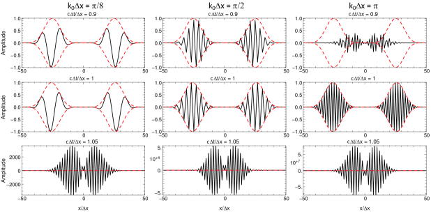
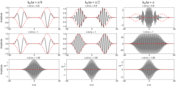
Snapshots from simulations using the Maxwell solver for various wavelengths and time steps are shown in Fig. 7, illustrating the findings of the numerical analysis. A driving signal is imposed on the field at the central grid point of the simulation grid, of the form where is the Harris function for and otherwise, with , and where is the number of grid cells. Plots are given for and .
For , the accuracy of the wave propagation deteriorates with increasing , to the point of being very inaccurate at the Nyquist limit. At , the pulses are correctly propagated, with the correct phase and amplitude, as expected. With , the instability of the solver is clearly visible, with the largest growth rate at the Nyquist wavelength .
One-dimensional wave solver with source term
While the analysis and the numerical experiment shows that the algorithm is stable and accurate for , it is illuminating to look at the response of the algorithm to a prescribed source term.
The wave equation with source term writes as:
| (28a) | ||||
| (28b) | ||||
Similarly to the particle pusher, this system of equations can easily be discretized using leapfrogged space- and time-centered finite-differencing, giving
| (29a) | ||||
| (29b) | ||||
Snapshots from simulations using the Maxwell solver with a prescribed source term, driven at various wavelengths and time steps are shown in Fig. 8. The most notable differences with the scheme without source is that the signal grows to larger amplitudes at the Nyquist wavelength, especially for . Indeed, analysis shows that the response of Eq. 29a-29b to a source oscillating at is of the form , exhibiting a linear amplitude growth in time. This indicates that when coupling with particles, it is important to remove any signal at the Nyquist wavelength. This can be done efficiently by applying a bilinear filter (see section 2.6) on the source term at each time step.
2.3.2 The Yee or Finite-Difference Time-Domain (FDTD) Maxwell solver
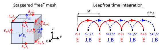
The most popular algorithm for electromagnetic PIC codes is the Yee, also known as Finite-Difference Time-Domain (or FDTD), solver [42]. It defines the electromagnetic field components on a staggered grid, such that all the operations in the discretized Maxwell’s equations are properly centered. The layout of the components is given in Fig. 9, where the electric field components are located between nodes and the magnetic field components are located in the center of the cell faces. The time integration follows the leapfrop scheme, where, knowing the current densities at half-integer steps, the electric field components are updated alternately with the magnetic field components at integer and half-integer steps respectively.
The algorithm can be written
| (30a) | |||||
| (30b) | |||||
with the following definitions of the operators:
| (31a) | |||||
| (31b) | |||||
| (31c) | |||||
| (31d) | |||||
| (31e) | |||||
where , , and are respectively the time step and the grid cell sizes along , and , respectively, and where is the time index and , and are the spatial indices along , and respectively.
For example, the update of is given explicitly by:
| (32) | ||||
| (33) | ||||
| (34) |
The updates for , , , and are obtained similarly.
Numerical accuracy and stability analysis A Von Neumann analysis leads to the following relation of dispersion
| (35a) | |||||
| (35b) | |||||
in two and three dimensions, respectively. This results in the following CFL conditions:
| (36a) | |||||
| (36b) | |||||
When and , the CFL conditions reduce to and in 2D and 3D, respectively.
The phase and group velocities are given respectively by
| (37a) | ||||
| (37b) | ||||
in 2-D, and
| (38a) | ||||
| (38b) | ||||
in 3-D.
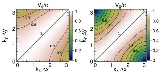
The maps of the 2-D phase and group velocities are plotted in Fig. 10, using the time step at the Courant limit , with . In this case, the phase and group velocities are exact for , i.e. for a planar wave propagating at 45 degrees from the grid axes. At other angles, both the phase and group velocities are below the physical value, down to and to for the phase and group velocities respectively, at the Nyquist wavelength along the grid axes.
In 3-D, the phase and group velocities are exact along the main diagonal of the grid when using the time step at the Courant limit , with . At other angles, both the phase and group velocities are below the physical value.
In the modeling of laser-driven plasma acceleration, it is convenient to launch the laser along one of the main axes, and the numerical dispersion of the Yee solver can lead to significant errors. To remedy this issue, it has become common to adopt solvers based on Non-Standard Finite-Difference Time-Domain (NSFDTD) or Pseudo-Spectral Analytical Time-Domain solvers, which will be presented next.
2.3.3 Non-Standard Finite-Difference Time-Domain (NSFDTD)
In [43, 44], Cole introduced an implementation of the source-free Maxwell’s wave equations for narrow-band applications based on non-standard finite-differences (NSFD). In [45], Karkkainen et al. adapted it for wideband applications. At the Courant limit for the time step and for a given set of parameters, the stencil proposed in [45] has no numerical dispersion along the principal axes, provided that the cell size is the same along each dimension (i.e. cubic cells in 3D). The “Cole-Karkkainnen” (or CK) solver uses the non-standard finite difference formulation (based on extended stencils) of the Maxwell-Ampere equation. The extension for electromagnetic PIC with the source term is given in [26] and reads:
| (39a) | |||||
| (39b) | |||||
The NSFD differential operator (see layout in Fig. 11) is given by
| (40) |
where
| (41) |
with
| (42a) | |||||
| (42b) | |||||
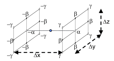
is a sample vector component, while , and are constant scalars satisfying . As with the FDTD algorithm, the quantities with half-integer are located between the nodes (electric field components) or in the center of the cell faces (magnetic field components). The operators along and , i.e. , , , , , , , and , are obtained by circular permutation of the indices.
For example, the update of is given explicitly by:
| (43) |
The updates of and are obtained by circular permutations. The updates of , and are the same as for the Yee algorithm.
Numerical accuracy and stability analysis A Von Neumann analysis leads to the following relation of dispersion
| (44a) | |||||
with
| (45a) | |||||
| (45b) | |||||
| (45c) | |||||
and
| (46a) | |||||
| (46b) | |||||
| (46c) | |||||
As shown in [45], assuming , and setting , and leads to a CFL limit of .
The maps of the 2-D phase and group velocities are plotted in Fig. 12, using the time step at the Courant limit , with . In this case, the phase and group velocities are exact along the main axes. At any angle from the axes, both the phase and group velocities are below the physical value, down to and to for the phase and group velocities respectively, at the Nyquist wavelength along the diagonal.
In 3-D, the phase and group velocities are exact along the main axes of the grid when using the time step at the Courant limit , with . At other angles, both the phase and group velocities are below the physical value.
Hence, assuming cubic cells (), the coefficients given in [45] (, and ) allow for the Courant condition to be at , which equates to having no numerical dispersion along the principal axes. The algorithm reduces to the FDTD algorithm with and . Prescriptions for the coefficients are provided by Cowan, et al. in 3-D in [46] and by Pukhov in 2-D in [47], that enable no numerical dispersion along the direction of the smallest cell size when using non-cubic cells. An alternative NSFDTD implementation that enables superluminous waves along one axis is also given by Lehe et al. in [48].
Enabling low or no numerical dispersion at all angles necessitates the use of higher-order finite-differences, which is more efficiently handled with Fourier-based spectral solvers.
2.3.4 Pseudo Spectral Analytical Time Domain (PSATD)
High-order approximations to the first spatial derivative can be obtained by using a larger stencil that involves more points on the grid. At the limit of infinite order, the approximate derivative is considered exact. It can be shown that at the limit of infinite order approximation of the spatial derivatives and infinitely small time steps, the algorithm is exact for all wavelengths and directions.
Even for high finite order and small, but finite, sub time steps, such an algorithm would be too costly and impractical. Solving instead Maxwell’s equation in Fourier space enables the evaluation of the derivative at any order, and analytical integration in time, thanks to the linearity of the equations.
Maxwell’s equations in Fourier space are given by
| (47a) | |||||
| (47b) | |||||
| (47c) | |||||
| (47d) | |||||
where is the Fourier Transform of the quantity . As with the real space formulation, provided that the continuity equation is satisfied, then the last two equations will automatically be satisfied at any time if satisfied initially and do not need to be explicitly integrated.
Decomposing the electric field and current between longitudinal and transverse components and gives
| (48a) | |||||
| (48b) | |||||
| (48c) | |||||
with .
If the sources are assumed to be constant over a time interval , the system of equations is solvable analytically and is given by (see [49] for the original formulation and [50] for a more detailed derivation):
| (49a) | |||||
| (49b) | |||||
| (49c) | |||||
with and .
Combining the transverse and longitudinal components gives
| (50a) | |||||
| (50b) | |||||
| (50c) | |||||
For fields generated by the source terms without the self-consistent dynamics of the charged particles, this algorithm is free of numerical dispersion and is not subject to a Courant condition. Furthermore, this solution is exact for any time step size, subject to the initial assumption that the current source is constant over that time step, which turns out to be a standard assumption in the Particle-In-Cell method.
The PSATD formulation that was just given applies to the field components located at the nodes of the grid. As noted in [51], they can also be easily recast on a staggered Yee grid by multiplication of the field components by the appropriate phase factors to shift them from the collocated to the staggered locations. The choice between a collocated and a staggered formulation is application-dependent.
Finite-order PSATD-p method
Spectral solvers used to be very popular in the years 1970s to early 1990s, before being replaced by finite-difference methods with the advent of parallel supercomputers that favored local methods. However, it was shown recently that standard domain decomposition with Fast Fourier Transforms that are local to each subdomain could be used effectively with PIC spectral methods [50], at the cost of truncation errors in the guard cells that could be neglected under some conditions. Furthermore, using very high - but finite - order enables the use of pseudo-spectral solver with ultrahigh accuracy and a compact support that permits domain decomposition and scaling to a very large number of subdomains, for parallel simulations on multiple computer nodes (see Section 3.4). A detailed analysis of the effectiveness of the method with exact evaluation of the magnitude of the effect of the truncation error is given in [52] for stencils of arbitrary order (up-to the infinite “spectral” order).
The PSATD algorithm is generalized to an arbitrary order by simply substituting the exact spatial derivatives in Fourier space by the representation of the -order finite-difference of the operator in Fourier space. I.e., the first derivative of the quantity along the axis in Fourier space is approximated by
| (51) |
with (for a staggered grid)
| (52) |
where is the Fornberg coefficients ([53]) at order . Similar approximations and are performed along the other axes.
The phase and group velocities for the 2-D PSATD solver at order , versus wavenumbers, are given in Fig. 13 (assuming discretization on a staggered grid). In that case, the phase and group velocities have very low numerical dispersion at all angles and a very wide fraction of the spectrum. Note that in this case, since the algorithm is based on an analytic integration in time, there is no CFL condition, and the phase and group velocities in vacuum are thus independent of the time step value.
2.4 Current deposition
The current densities are deposited on the computational grid from the particle position and velocities, employing splines of various orders [54].
| (53a) | |||||
where is a spline of order that is given by the convolution of the rectangular function by itself. Hence, the Fourier transform of the spline of order is given by
| (54) |
In most applications, it is essential to prevent the accumulation of errors resulting from the violation of the discretized Gauss’ Law. This is accomplished by providing a method for depositing the current from the particles to the grid that preserves the discretized Gauss’ Law, or by providing a mechanism for “divergence cleaning” [38, 55, 56, 57, 58]. For the former, schemes that allow a deposition of the current that is exact when combined with the Yee solver is given in [59] for linear splines and in [60] for splines of arbitrary order.
Note that the NSFDTD formulations given above and in [47, 26, 46, 48] apply to the Maxwell-Faraday equation, while the discretized Maxwell-Ampere equation uses the FDTD formulation. Consequently, the charge conserving algorithms developed for current deposition [59, 60] apply readily to those NSFDTD-based formulations.
2.5 Field gather
In general, the field is gathered from the mesh onto the macroparticles using splines of the same order as for the current deposition . Two variations are considered:
-
•
“energy conserving”: fields are interpolated from the staggered Yee grid to the macroparticles using for , for , for , for , for and for ,
-
•
“momentum conserving”: fields are interpolated from the grid nodes to the macroparticles using for all field components (since the fields are known at staggered positions, they are first interpolated to the nodes, usually using linear interpolation).
Diagrams illustrating the two schemes in the standard case of linear splines () are given in Fig.15.
As shown in [38, 61, 62], the energy and momentum conserving schemes conserve energy or momentum respectively at the limit of infinitesimal time steps and generally offer better conservation of the respective quantities for a finite time step. Neither method is intrinsically superior to the other, and it can be useful to implement both methods and test whether one converges faster than the other for a given class of problems.
2.6 Filtering
It is common practice to apply digital filtering to the current density in Particle-In-Cell simulations as a complement or an alternative to using higher order splines [38]. As seen above in the section on the field solvers, the group velocity often vanishes at the Nyquist wavelength, and the Leapfrog Maxwell integrator is not stable at this wavelength. It is thus prudent to completely remove the Nyquist wavelength from the source term. Since the group velocity of the neighboring wavelengths are usually very inaccurate, it may also be beneficial to damp them.

A commonly used filter in PIC simulations is the three points filter
| (56) |
where is the filtered quantity. This filter is called a “bilinear” filter when . Assuming and , the filter gain is given as a function of the filtering coefficient and the wavenumber by
| (57) |
The total attenuation for successive applications of filters of coefficients … is given by . A sharper cutoff in space is provided by using , so that . Such step is called a “compensation” step [38]. For the bilinear filter (), the compensation factor is . For a succession of applications of the bilinear factor, it is .
Examples of gains of commonly used filters are shown in Fig.16.
2.7 Energy and momentum conservation

As mentioned above, and discussed in detail in [38, 61], there are schemes that can preserve energy or momentum, but only at the infinitesimal limit. When using finite time steps, as required in practice, neither is strictly preserved. It is thus important to have in mind these limitations and explore what set of parameters work best for a given problem.
To illustrate the energy and momentum conservation properties of the standard PIC using the Yee algorithms, histories of the global energy and momentum are given in Fig. 17 from simulations of a uniform warm plasma at rest, using either the “energy-conserving” or the “momentum-conserving” algorithm with deposition and gathering splines of orders 1 (linear), 2 (quadratic) or 3 (cubic).
As expected, the simulations using the “energy-conserving” gather do better at preserving the energy while the ones using the “momentum-conserving” gather preserved the momentum better. As explained above, the linear growth of energy is due to numerical “stochastic heating” from random errors from the fields acting on the particle motion. Using higher order splines reduces the magnitude of these random errors and thus the growth rate [54, 61, 38].
3 Application to the modeling of plasma-based accelerators
3.1 Moving window and optimal Lorentz boosted frame
The simulations of plasma accelerators from first principles are extremely computationally intensive, due to the need to resolve the evolution of a driver (laser or particle beam) and an accelerated particle beam into a plasma structure that is orders of magnitude longer and wider than the accelerated beam. As is customary in the modeling of particle beam dynamics in standard particle accelerators, a moving window is commonly used to follow the driver, the wake and the accelerated beam. This results in huge savings, by avoiding the meshing of the entire plasma that is orders of magnitude longer than the other length scales of interest.
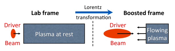
Even using a moving window, however, a full PIC simulation of a plasma accelerator can be extraordinarily demanding computationally, as many time steps are needed to resolve the crossing of the short driver beam with the plasma column. As it turns out, choosing an optimal frame of reference that travels close to the speed of light in the direction of the laser or particle beam (as opposed to the usual choice of the laboratory frame) enables speedups by orders of magnitude [17, 28]. This is a result of the properties of Lorentz contraction and dilation of space and time. In the frame of the laboratory, a very short driver (laser or particle) beam propagates through a much longer plasma column, necessitating millions to tens of millions of time steps for parameters in the range of the BELLA or FACET-II experiments. As sketched in Fig. 18, in a frame moving with the driver beam in the plasma at velocity (where is the speed of light in vacuum), the beam length is now elongated by while the plasma contracts by (where is the relativistic factor associated with the frame velocity). The number of time steps that is needed to simulate a “longer” beam through a “shorter” plasma is now reduced by up to (a detailed derivation of the speedup is given in [28]). For simulations of multi-GeV stages in the linear regime, the group velocity of the laser can reach , leading to speedups .
The modeling of a plasma acceleration stage in a boosted frame involves the fully electromagnetic modeling of a plasma propagating at near the speed of light, for which Numerical Cerenkov [63, 49] is a potential issue, as explained in more details below. In addition, for a frame of reference moving in the direction of the accelerated beam (or equivalently the wake of the laser), waves emitted by the plasma in the forward direction expand while the ones emitted in the backward direction contract, following the properties of the Lorentz transformation. If one had to resolve both forward and backward propagating waves emitted from the plasma, there would be no gain in selecting a frame different from the laboratory frame. However, the physics of interest for a laser wakefield is the laser driving the wake, the wake, and the accelerated beam. Backscatter is weak in the short-pulse regime, and does not interact as strongly with the beam as do the forward propagating waves which stay in phase for a long period. It is thus often assumed that the backward propagating waves can be neglected in the modeling of plasma accelerator stages. The accuracy of this assumption has been demonstrated by comparison between explicit codes that include both forward and backward waves with envelope or quasistatic codes that neglect backward waves [2, 37, 64].
3.2 Numerical Cherenkov Instability and alternate formulation in a Galilean frame
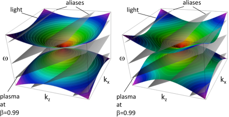
The “Numerical Cherenkov Instability” (NCI) [65] is the most serious numerical instability affecting multidimensional PIC simulations of relativistic particle beams and streaming plasmas [25, 22, 26, 66, 67, 68]. It arises from coupling between possibly numerically distorted electromagnetic modes and spurious beam modes, the latter due to the mismatch between the Lagrangian treatment of particles and the Eulerian treatment of fields [69] (See Fig. 19). In recent papers, the electromagnetic dispersion relations for the numerical Cherenkov instability were derived and solved for both FDTD [67, 70] and PSATD [71, 72] algorithms.
Several solutions have been proposed to mitigate the NCI [73, 72, 71, 74, 75, 76]. Although these solutions reduce efficiently the growth rate of the numerical instability, they typically introduce either strong smoothing of the currents and fields, or arbitrary numerical corrections, which are tuned specifically against the NCI and go beyond the natural discretization of the underlying physical equation. Therefore, it is sometimes unclear to what extent these added corrections could impact the physics at stake for a given resolution.
For instance, NCI-specific corrections include periodically smoothing the electromagnetic field components [25], using a special time step [22, 26] or applying a wide-band smoothing of the current components [22, 26, 27]. Another set of mitigation methods involves scaling the deposited currents by a carefully-designed wavenumber-dependent factor [70, 72] or slightly modifying the ratio of electric and magnetic fields () before gathering their value onto the macroparticles [71, 74]. Yet another set of NCI-specific corrections [75, 76] consists in combining a small timestep , a sharp low-pass spatial filter, and a spectral or high-order scheme that is tuned so as to create a small, artificial “bump” in the dispersion relation [75]. While most mitigation methods have only been applied to Cartesian geometry, this last set of methods ([75, 76]) has the remarkable property that it can be applied [76] to both Cartesian geometry and quasi-cylindrical geometry (i.e. cylindrical geometry with azimuthal Fourier decomposition [31, 32, 33]). However, the use of a small timestep proportionally slows down the progress of the simulation, and the artificial “bump” is again an arbitrary correction that departs from the underlying physics.
A new scheme was recently proposed, in [77, 78], which completely eliminates the NCI for a plasma drifting at a uniform relativistic velocity – with no arbitrary correction – by simply integrating the PIC equations in Galilean coordinates (also known as comoving coordinates). More precisely, in the new method, the Maxwell equations in Galilean coordinates are integrated analytically, using only natural hypotheses, within the PSATD framework (Pseudo-Spectral-Analytical-Time-Domain [49, 79]).
The idea of the proposed scheme is to perform a Galilean change of coordinates, and to carry out the simulation in the new coordinates:
| (58) |
where and are the position vectors in the standard and Galilean coordinates respectively. The new equations and algorithm derived in the Galilean frame are given in Appendix C.
As shown in [77, 78], the elimination of the NCI with the new Galilean integration is verified empirically via PIC simulations of uniform drifting plasmas and laser-driven plasma acceleration stages, and confirmed by a theoretical analysis of the instability.
When choosing , where is the speed of the bulk of the relativistic plasma, the plasma does not move with respect to the grid in the Galilean coordinates – or, equivalently, in the standard coordinates , the grid moves along with the plasma. The heuristic intuition behind this scheme is that these coordinates should prevent the discrepancy between the Lagrangian and Eulerian point of view, which gives rise to the NCI [69].
An important remark is that the Galilean change of coordinates (58) is a simple translation. Thus, when used in the context of Lorentz-boosted simulations, it does of course preserve the relativistic dilatation of space and time which gives rise to the characteristic computational speedup of the boosted-frame technique.
Another important remark is that the Galilean scheme is not equivalent to a moving window (and in fact the Galilean scheme can be independently combined with a moving window). Whereas in a moving window, gridpoints are added and removed so as to effectively translate the boundaries, in the Galilean scheme the gridpoints themselves are not only translated but in this case, the physical equations are modified accordingly. Most importantly, the assumed time evolution of the current within one timestep is different in a standard PSATD scheme with moving window and in a Galilean PSATD scheme [78].
3.3 Examples
3.3.1 3-D example of LWFA and PWFA

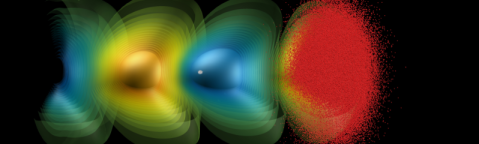
The application of the standard electromagnetic PIC method is illustrated here with 3-D simulations of a laser-driven and a charged-particle-beam-driven plasma accelerator. Renderings are shown in Fig. 20, showing the driver beams and the wakes created by the driver propagating through the plasma column.
These examples are from simulations using a moving window in the laboratory frame. They used the Yee Maxwell solver, “energy-conserving” gather, splines of order 3 and smoothing in the longitudinal direction (4 passes of bilinear filter + 1 pass of compensation).
3.3.2 Diagnostics from boosted frame simulations
As explained above, simulating in a Lorentz boosted frame can speedup the simulations by orders of magnitude when using extra precaution to control the numerical Cherenkov instability. In addition, input and output need special treatment to convert the input data from the laboratory frame to the boosted frame and the output data from the boosted frame to the laboratory.
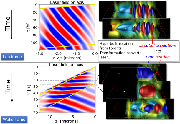
In addition to analyzing the output data in the laboratory frame, it is instructive to analyze the data in the boosted frame, as the physics looks different and may lead to alternate insight for the physical phenomena as well as for numerical considerations. It is especially true for the modeling of laser-driven plasma accelerators, where the group velocity of the laser in the plasma is usually low enough to be used as the Lorentz boosted frame.
This is illustrated in Fig. 21 that shows snapshots of the same 3-D simulation of the previous section in the laboratory frame, as well as from a simulation of the same setup in a Lorentz boosted frame propagating at the group velocity of the laser in the plasma. The time histories of the laser field oscillations on axis are also shown for each simulation. While spatial laser oscillations are clearly visible while the laser is propagating through the plasma in the laboratory frame simulation, the hyperbolic rotation of the Lorentz transformation converts them into pure time beating while the laser is propagating through the plasma in the boosted frame simulation. The usual spatial oscillations naturally occur again as the laser exits the plasma. One important consequence of this observation is that the relative content in short wavelength is reduced in boosted frame simulations, enabling more aggressive smoothing (if needed) [27] or potentially a coarser longitudinal resolution (relative to the laser wavelength in vacuum).
3.3.3 Convergence
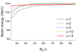

Given that all PIC simulations are approximations of the real system, it is essential to conduct convergence studies with regard to mesh size in every direction, number of macroparticles and time step size. An example of convergence study, using the final accelerated electron beam energy and transverse emittance as metrics, is shown in Fig. 22 as the longitudinal resolution is varied between 24 and 96 mesh points per laser wavelength. The transverse resolution was kept constant, as well as the total number of macroparticles in the accelerated electron beam. The number of macroparticles of plasma per cell was also kept constant, hence the total number of plasma macroparticles was rising with the longitudinal resolution. The time step was adjusted automatically relative to the CFL limit and was thus decreased as the longitudinal resolution was decreased. The study was repeated for various values of the relativistic factor of the Lorentz boosted frame of the simulation.
Both the beam energy and emittance converge nicely as the longitudinal resolution is increased. However, they do not converge to the same value in each boosted frame. This is an indication that the simulation is not converge along all its components, hence most likely with regard to the transverse resolution as it was kept constant in this study. Increasing the transverse resolution did indeed improve the convergence in this case. Convergence of plasma acceleration simulations can be even more demanding for simulations that involve trapping, such as for the study of injection scheme. A detailed study of convergence of boosted frame simulations of a laser-driven injection scheme is given in [80].
3.3.4 Mesh refinement
With the standard PIC method, the entire simulation domain is covered with a grid at the same resolution everywhere, regardless of the underlying physical spatial scales. Hence, the grid cell must be a fraction of the smallest spatial feature to be resolved. If the concerned volume is only a small subset of the entire domain, it can be very expensive.
There are typically two approaches to enable variable resolution: mesh refinement of Cartesian meshes or use of irregular meshes (often with the finite element method). The PIC extension to irregular meshes is quite complicated, and the tracking of macroparticles through an irregular mesh tends to be very expensive. We will thus concentrate here on mesh refinement.
Mesh refinement (MR) is quite common in fluid dynamics but much less in electromagnetic simulations, especially when coupled to particles as with the electromagnetic PIC method. One reason is that standard MR methods, which are based on interpolation of field quantities between grids at different resolution, do cause reflection with amplification of electromagnetic modes that are resolved on the finer grid but not on the coarser one. To make matters worse, the reflection is typically associated with amplification [81]. Hence, using standard MR method that are based on interpolation between grids with the electromagnetic PIC code leads to unstable methods or need a very high level of numerical damping to stabilize the system, with an associated cost on physical accuracy.
Several methods have been proposed to add MR to electromagnetic PIC without interpolation between fields at different levels of refinement [82, 83, 84, 85]. In [82, 83], the linearity of Maxwell’s equation is used to decouple the field solution in the MR area in three parts: parent grid, coarse patch and fine patch. In this scheme, the update of Maxwell’s equations on the parent grid is done without modification of the standard PIC. The effect of MR is accounted for by adding a “correction” from the combination of the field computed on the coarse and fine patches, each surrounded by Perfectly Matched Layers [86] to absorb all outgoing waves, avoiding spurious reflections.
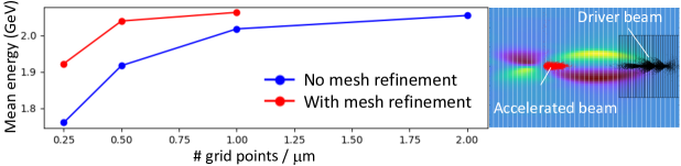
An example of 3-D simulation using this method is shown in Fig. 23, where the formation of the wake by a charged particle beam is highly sensitive to the grid resolution. A refinement patch is thus applied on the volume occupied by the driver beam. The benefit of mesh refinement is measured on the dependency of the accelerated beam moments with regard to grid resolution on the parent. In this particular example, the application of the MR patch around the driver beam only enables convergence to a precision nearly identical to the one obtained using a fine grid covering the entire simulation domain.
3.4 High-performance computing
Even using the Lorentz boosted frame technique, mesh refinement, reduced dimensions by expanding the fields into a truncated series of azimuthal modes, the quasistatic approximation, ponderomotive guiding center (PGC) models, or combination of these or other advanced algorithms, the modeling of plasma accelerators is computationally very demanding and often calls for high-performance computing. This is especially true for the potential future application of plasma accelerators to high-energy physics colliders, where chains of tens to thousands of multi-GeV plasma accelerators are needed to reach multi-TeV energy range in the center of mass of the collision.
The codes that are used for the modeling of plasma accelerators are thus in general parallelized, to enable the use of many computer nodes at once. The parallelization is usually based on domain decomposition, where the simulation domain is decomposed in subdomains, each handled by one computer nodes. The decomposition is typically uniform Cartesian and the same for fields and particles. At each time step, field information is needed from neighboring nodes to compute the finite spatial derivatives of fields on the grid, in order to update the Maxwell field solver to the next time step. Hence, messages are sent and received between neighboring nodes that contain the field information that is needed for the update. Similarly, macroparticles may move from one subdomain to another and need to be passed via message passing. Since the distribution of macroparticles may evolve during the simulations and may be highly non-uniform (e.g. the plasma electrons in the bubble regime), a uniform Cartesian domain decomposition is not always optimal. Hence, irregular domain decomposition (which may also be different for fields and particles) is needed, with periodic remapping to enable dynamic load balancing among computer nodes.
In addition, each computer node may contain multiple processor units, including graphical processing units (GPUs). This requires additional levels of parallelization and writing of portions of codes using annotations and language extensions. The writing of codes that are fully optimized with multiple levels of parallelisms and can scale to many nodes has thus become very specialized, and it is sometimes handled by teams of two or more.
4 Outlook
The development of plasma-based accelerators, and in particular high-energy physics colliders, depends critically on high-performance, high-fidelity modeling to capture the full complexity of acceleration processes that develop over a large range of space and time scales. The field will continue to be a driver for pushing the state-of-the-art in the detailed modeling of relativistic plasmas. The modeling of tens to thousands of multi-GeV stages, as envisioned for plasma-based high-energy physics colliders, will require further advances in algorithmic, and depends critically on codes’ readiness for the upcoming era of exascale supercomputing. This requires coordination within the community with team efforts.
The emergence of standards for the output data (e.g. the open Particle Mesh Data - or openPMD - standard) and code inputs (e.g. the Particle-In-Cell Modeling Interface - or PICMI - standard), if successfully adopted, can pave the way for an integrated ecosystem of new breeds of codes that would great simplify the work of many developers and users, thereby leading to speed up of discovery and novel designs of plasma accelerators that would not be possible otherwise. Standardization of output data will also greatly facilitate a systematic and coordinated development and adoption of ultrafast Machine Learning surrogate models for real-time optimization and control of particle accelerators from simulation (and experimental) data, with a potential for dramatic acceleration of discovery.
Further down the road, the emerging and largely unexplored area of quantum computing offers new opportunities for the modeling of plasma accelerators that are yet to be imagined.
Acknowledgements
I would like to thank all my mentors, collaborators, colleagues and students who have taught me, pushed me to learn deeper and are continuously driving us toward more understanding, novel solutions and new questions.
This work was supported by US-DOE Contract DE-AC02-05CH11231 and by the Exascale Computing Project (17-SC-20-SC), a collaborative effort of the U.S. Department of Energy Office of Science and the National Nuclear Security Administration.
References
- [1] Fs Tsung, W Lu, M Tzoufras, Wb Mori, C Joshi, Jm Vieira, Lo Silva, and Ra Fonseca. Simulation Of Monoenergetic Electron Generation Via Laser Wakefield Accelerators For 5-25 Tw Lasers. Physics Of Plasmas, 13(5):56708, may 2006.
- [2] C G R Geddes, D L Bruhwiler, J R Cary, W B Mori, J.-L. Vay, S F Martins, T Katsouleas, E Cormier-Michel, W M Fawley, C Huang, X Wang, B Cowan, V K Decyk, E Esarey, R A Fonseca, W Lu, P Messmer, P Mullowney, K Nakamura, K Paul, G R Plateau, C B Schroeder, L O Silva, C Toth, F S Tsung, M Tzoufras, T Antonsen, J Vieira, and W P Leemans. Computational Studies And Optimization Of Wakefield Accelerators. In Journal of Physics: Conference Series, volume 125, page 012002 (11 Pp.), 2008.
- [3] Cgr Geddes It Et Al. Laser Plasma Particle Accelerators: Large Fields For Smaller Facility Sources. In Scidac Review 13, page 13, 2009.
- [4] C Huang, W An, V K Decyk, W Lu, W B Mori, F S Tsung, M Tzoufras, S Morshed, T Antonsen, B Feng, T Katsouleas, R A Fonseca, S F Martins, J Vieira, L O Silva, E Esarey, C G R Geddes, W P Leemans, E Cormier-Michel, J.-L. Vay, D L Bruhwiler, B Cowan, J R Cary, and K Paul. Recent Results And Future Challenges For Large Scale Particle-In-Cell Simulations Of Plasma-Based Accelerator Concepts. Journal of Physics: Conference Series, 180(1):012005 (11 Pp.), 2009.
- [5] W P Leemans, A J Gonsalves, H.-S. Mao, K Nakamura, C Benedetti, C B Schroeder, Cs. Tóth, J Daniels, D E Mittelberger, S S Bulanov, J.-L. Vay, C G R Geddes, and E Esarey. Multi-GeV Electron Beams from Capillary-Discharge-Guided Subpetawatt Laser Pulses in the Self-Trapping Regime. Phys. Rev. Lett., 113(24):245002, dec 2014.
- [6] Ian Blumenfeld, Christopher E Clayton, Franz-Josef Decker, Mark J Hogan, Chengkun Huang, Rasmus Ischebeck, Richard Iverson, Chandrashekhar Joshi, Thomas Katsouleas, Neil Kirby, Wei Lu, Kenneth A Marsh, Warren B Mori, Patric Muggli, Erdem Oz, Robert H Siemann, Dieter Walz, and Miaomiao Zhou. Energy doubling of 42[thinsp]GeV electrons in a metre-scale plasma wakefield accelerator. Nature, 445(7129):741–744, feb 2007.
- [7] Bulanov S V and Wilkens J J and Esirkepov T Zh and Korn G and Kraft G and Kraft S D and Molls M and Khoroshkov V S. Laser ion acceleration for hadron therapy. Physics-Uspekhi, 57(12):1149, 2014.
- [8] S Steinke, J van Tilborg, C Benedetti, C G R Geddes, C B Schroeder, J Daniels, K K Swanson, A J Gonsalves, K Nakamura, N H Matlis, B H Shaw, E Esarey, and W P Leemans. Multistage coupling of independent laser-plasma accelerators. Nature, 530(7589):190–193, feb 2016.
- [9] A. J. Gonsalves, K. Nakamura, J. Daniels, C. Benedetti, C. Pieronek, T. C.H. De Raadt, S. Steinke, J. H. Bin, S. S. Bulanov, J. Van Tilborg, C. G.R. Geddes, C. B. Schroeder, Cs Tóth, E. Esarey, K. Swanson, L. Fan-Chiang, G. Bagdasarov, N. Bobrova, V. Gasilov, G. Korn, P. Sasorov, and W. P. Leemans. Petawatt Laser Guiding and Electron Beam Acceleration to 8 GeV in a Laser-Heated Capillary Discharge Waveguide. Physical Review Letters, 122(8), feb 2019.
- [10] P Sprangle, E Esarey, and A Ting. Nonlinear-Theory Of Intense Laser-Plasma Interactions. Physical Review Letters, 64(17):2011–2014, apr 1990.
- [11] T M Antonsen and P Mora. Self-Focusing And Raman-Scattering Of Laser-Pulses In Tenuous Plasmas. Physical Review Letters, 69(15):2204–2207, oct 1992.
- [12] J Krall, A Ting, E Esarey, and P Sprangle. Enhanced Acceleration In A Self-Modulated-Laser Wake-Field Accelerator. Physical Review E, 48(3):2157–2161, sep 1993.
- [13] P Mora and Tm Antonsen. Kinetic Modeling Of Intense, Short Laser Pulses Propagating In Tenuous Plasmas. Phys. Plasmas, 4(1):217–229, jan 1997.
- [14] C Huang, V K Decyk, C Ren, M Zhou, W Lu, W B Mori, J H Cooley, T M Antonsen Jr., and T Katsouleas. Quickpic: A Highly Efficient Particle-In-Cell Code For Modeling Wakefield Acceleration In Plasmas. Journal of Computational Physics, 217(2):658–679, sep 2006.
- [15] C Benedetti, C B Schroeder, E Esarey, C G R Geddes, and W P Leemans. Efficient Modeling Of Laser-Plasma Accelerators With Inf&Rno. Aip Conference Proceedings, 1299:250–255, 2010.
- [16] Benjamin M Cowan, David L Bruhwiler, Estelle Cormier-Michel, Eric Esarey, Cameron G R Geddes, Peter Messmer, and Kevin M Paul. Characteristics Of An Envelope Model For Laser-Plasma Accelerator Simulation. Journal of Computational Physics, 230(1):61–86, 2011.
- [17] J.-L. Vay. Noninvariance Of Space- And Time-Scale Ranges Under A Lorentz Transformation And The Implications For The Study Of Relativistic Interactions. Physical Review Letters, 98(13):130405/1–4, 2007.
- [18] D L Bruhwiler, J R Cary, B M Cowan, K Paul, C G R Geddes, P J Mullowney, P Messmer, E Esarey, E Cormier-Michel, W Leemans, and J.-L. Vay. New Developments In The Simulation Of Advanced Accelerator Concepts. In Aip Conference Proceedings, volume 1086, pages 29–37, 2009.
- [19] J.-L. Vay, D L Bruhwiler, C G R Geddes, W M Fawley, S F Martins, J R Cary, E Cormier-Michel, B Cowan, R A Fonseca, M A Furman, W Lu, W B Mori, and L O Silva. Simulating Relativistic Beam And Plasma Systems Using An Optimal Boosted Frame. Journal of Physics: Conference Series, 180(1):012006 (5 Pp.), 2009.
- [20] J.-L. Vay it Et Al. Application Of The Reduction Of Scale Range In A Lorentz Boosted Frame To The Numerical Simulation Of Particle Acceleration Devices. In Proc. Particle Accelerator Conference, Vancouver, Canada, 2009.
- [21] S F Martins It Et Al. Boosted Frame Pic Simulations Of Lwfa: Towards The Energy Frontier. In Proc. Particle Accelerator Conference, Vancouver, Canada, 2009.
- [22] J . L Vay, C G R Geddes, C Benedetti, D L Bruhwiler, E Cormier-Michel, B M Cowan, J R Cary, and D P Grote. Modeling Laser Wakefield Accelerators In A Lorentz Boosted Frame. Aip Conference Proceedings, 1299:244–249, 2010.
- [23] S F Martins, R A Fonseca, W Lu, W B Mori, and L O Silva. Exploring Laser-Wakefield-Accelerator Regimes For Near-Term Lasers Using Particle-In-Cell Simulation In Lorentz-Boosted Frames. Nature Physics, 6(4):311–316, apr 2010.
- [24] S F Martins, R A Fonseca, J Vieira, L O Silva, W Lu, and W B Mori. Modeling Laser Wakefield Accelerator Experiments With Ultrafast Particle-In-Cell Simulations In Boosted Frames. Physics Of Plasmas, 17(5):56705, may 2010.
- [25] Samuel F Martins, Ricardo A Fonseca, Luis O Silva, Wei Lu, and Warren B Mori. Numerical Simulations Of Laser Wakefield Accelerators In Optimal Lorentz Frames. Computer Physics Communications, 181(5):869–875, may 2010.
- [26] J L Vay, C G R Geddes, E Cormier-Michel, and D P Grote. Numerical Methods For Instability Mitigation In The Modeling Of Laser Wakefield Accelerators In A Lorentz-Boosted Frame. Journal of Computational Physics, 230(15):5908–5929, jul 2011.
- [27] Jl Vay, C G R Geddes, E Cormier-Michel, and D P Grote. Effects Of Hyperbolic Rotation In Minkowski Space On The Modeling Of Plasma Accelerators In A Lorentz Boosted Frame. Physics Of Plasmas, 18(3):30701, mar 2011.
- [28] J L. Vay, C G R Geddes, E Esarey, C B Schroeder, W P Leemans, E Cormier-Michel, and D P Grote. Modeling Of 10 Gev-1 Tev Laser-Plasma Accelerators Using Lorentz Boosted Simulations. Physics Of Plasmas, 18(12), dec 2011.
- [29] Peicheng Yu, Xinlu Xu, Asher Davidson, Adam Tableman, Thamine Dalichaouch, Fei Li, Michael D. Meyers, Weiming An, Frank S. Tsung, Viktor K. Decyk, Frederico Fiuza, Jorge Vieira, Ricardo A. Fonseca, Wei Lu, Luis O. Silva, and Warren B. Mori. Enabling Lorentz boosted frame particle-in-cell simulations of laser wakefield acceleration in quasi-3D geometry. Journal of Computational Physics, 316:747–759, jul 2016.
- [30] B B Godfrey and MISSION RESEARCH CORP ALBUQUERQUE NM. The IPROP Three-Dimensional Beam Propagation Code. Defense Technical Information Center, 1985.
- [31] A F Lifschitz, X Davoine, E Lefebvre, J Faure, C Rechatin, and V Malka. Particle-in-Cell modelling of laser plasma interaction using Fourier decomposition. Journal of Computational Physics, 228(5):1803–1814, 2009.
- [32] A. Davidson, A. Tableman, W. An, F.S. Tsung, W. Lu, J. Vieira, R.A. Fonseca, L.O. Silva, and W.B. Mori. Implementation of a hybrid particle code with a PIC description in r–z and a gridless description in into OSIRIS. Journal of Computational Physics, 281:1063–1077, 2015.
- [33] Rémi Lehe, Manuel Kirchen, Igor A. Andriyash, Brendan B. Godfrey, and Jean-Luc Vay. A spectral, quasi-cylindrical and dispersion-free Particle-In-Cell algorithm. Computer Physics Communications, 203:66–82, 2016.
- [34] Igor A. Andriyash, Remi Lehe, and Agustin Lifschitz. Laser-plasma interactions with a Fourier-Bessel particle-in-cell method. Physics of Plasmas, 23(3), mar 2016.
- [35] B A Shadwick, C B Schroeder, and E Esarey. Nonlinear Laser Energy Depletion In Laser-Plasma Accelerators. Physics Of Plasmas, 16(5):56704, may 2009.
- [36] E Cormier-Michel, C G R Geddes, E Esarey, C B Schroeder, D L Bruhwiler, K Paul, B Cowan, and W P Leemans. Scaled Simulations Of A 10 Gev Accelerator. In Aip Conference Proceedings, volume 1086, pages 297–302, 2009.
- [37] C G R Geddes It Et Al. Scaled Simulation Design Of High Quality Laser Wakefield Accelerator Stages. In Proc. Particle Accelerator Conference, Vancouver, Canada, 2009.
- [38] C K Birdsall and A B Langdon. Plasma Physics Via Computer Simulation. Adam-Hilger, 1991.
- [39] Jp Boris. Relativistic Plasma Simulation-Optimization of a Hybrid Code. In Proc. Fourth Conf. Num. Sim. Plasmas, pages 3–67, Naval Res. Lab., Wash., D. C., 1970.
- [40] J L Vay. Simulation Of Beams Or Plasmas Crossing At Relativistic Velocity. Physics Of Plasmas, 15(5):56701, may 2008.
- [41] A. V. Higuera and J. R. Cary. Structure-preserving second-order integration of relativistic charged particle trajectories in electromagnetic fields. Physics of Plasmas, 24(5), may 2017.
- [42] Ks Yee. Numerical Solution Of Initial Boundary Value Problems Involving Maxwells Equations In Isotropic Media. Ieee Transactions On Antennas And Propagation, Ap14(3):302–307, 1966.
- [43] Jb Cole. A High-Accuracy Realization Of The Yee Algorithm Using Non-Standard Finite Differences. Ieee Transactions On Microwave Theory And Techniques, 45(6):991–996, jun 1997.
- [44] Jb Cole. High-Accuracy Yee Algorithm Based On Nonstandard Finite Differences: New Developments And Verifications. Ieee Transactions On Antennas And Propagation, 50(9):1185–1191, sep 2002.
- [45] M Karkkainen, E Gjonaj, T Lau, and T Weiland. Low-Dispersionwake Field Calculation Tools. In Proc. Of International Computational Accelerator Physics Conference, pages 35–40, Chamonix, France, 2006.
- [46] Benjamin M Cowan, David L Bruhwiler, John R Cary, Estelle Cormier-Michel, and Cameron G R Geddes. Generalized algorithm for control of numerical dispersion in explicit time-domain electromagnetic simulations. Physical Review Special Topics-Accelerators And Beams, 16(4), apr 2013.
- [47] A Pukhov. Three-dimensional electromagnetic relativistic particle-in-cell code VLPL (Virtual Laser Plasma Lab). Journal of Plasma Physics, 61(3):425–433, apr 1999.
- [48] R Lehe, A Lifschitz, C Thaury, V Malka, and X Davoine. Numerical growth of emittance in simulations of laser-wakefield acceleration. Physical Review Special Topics - Accelerators and Beams, 16(2):021301, feb 2013.
- [49] I Haber, R Lee, Hh Klein, and Jp Boris. Advances In Electromagnetic Simulation Techniques. In Proc. Sixth Conf. Num. Sim. Plasmas, pages 46–48, Berkeley, Ca, 1973.
- [50] Jean-Luc Vay, Irving Haber, and Brendan B Godfrey. A domain decomposition method for pseudo-spectral electromagnetic simulations of plasmas. Journal of Computational Physics, 243:260–268, jun 2013.
- [51] Y Ohmura and Y Okamura. Staggered Grid Pseudo-Spectral Time-Domain Method For Light Scattering Analysis. Piers Online, 6(7):632–635, 2010.
- [52] H. Vincenti and J.-L. Vay. Detailed analysis of the effects of stencil spatial variations with arbitrary high-order finite-difference Maxwell solver. Computer Physics Communications, 200:147–167, mar 2016.
- [53] Bengt Fornberg. High-order finite differences and the pseudospectral method on staggered grids. SIAM Journal on Numerical Analysis, 27(4):904–918, 1990.
- [54] H Abe, N Sakairi, R Itatani, and H Okuda. High-Order Spline Interpolations In The Particle Simulation. Journal of Computational Physics, 63(2):247–267, apr 1986.
- [55] A B Langdon. On Enforcing Gauss Law In Electromagnetic Particle-In-Cell Codes. Computer Physics Communications, 70(3):447–450, jul 1992.
- [56] B Marder. A Method For Incorporating Gauss Law Into Electromagnetic Pic Codes. Journal of Computational Physics, 68(1):48–55, jan 1987.
- [57] J.-L. Vay and C Deutsch. Charge Compensated Ion Beam Propagation In A Reactor Sized Chamber. Physics Of Plasmas, 5(4):1190–1197, apr 1998.
- [58] Cd Munz, P Omnes, R Schneider, E Sonnendrucker, and U Voss. Divergence Correction Techniques For Maxwell Solvers Based On A Hyperbolic Model. Journal of Computational Physics, 161(2):484–511, jul 2000.
- [59] J Villasenor and O Buneman. Rigorous Charge Conservation For Local Electromagnetic-Field Solvers. Computer Physics Communications, 69(2-3):306–316, 1992.
- [60] Tz Esirkepov. Exact Charge Conservation Scheme For Particle-In-Cell Simulation With An Arbitrary Form-Factor. Computer Physics Communications, 135(2):144–153, apr 2001.
- [61] R W Hockney and J W Eastwood. Computer simulation using particles. 1988.
- [62] H.Ralph Lewis. Variational algorithms for numerical simulation of collisionless plasma with point particles including electromagnetic interactions. Journal of Computational Physics, 10(3):400–419, 1972.
- [63] Jp Boris and R Lee. Nonphysical Self Forces In Some Electromagnetic Plasma-Simulation Algorithms. Journal of Computational Physics, 12(1):131–136, 1973.
- [64] B Cowan, D Bruhwiler, E Cormier-Michel, E Esarey, C G R Geddes, P Messmer, and K Paul. Laser Wakefield Simulation Using A Speed-Of-Light Frame Envelope Model. In Aip Conference Proceedings, volume 1086, pages 309–314, 2009.
- [65] Bb Godfrey. Numerical Cherenkov Instabilities In Electromagnetic Particle Codes. Journal of Computational Physics, 15(4):504–521, 1974.
- [66] L Sironi and A Spitkovsky. No Title, 2011.
- [67] Brendan B Godfrey and Jean-Luc Vay. Numerical stability of relativistic beam multidimensional {PIC} simulations employing the Esirkepov algorithm. Journal of Computational Physics, 248(0):33–46, 2013.
- [68] Xinlu Xu, Peicheng Yu, Samual F Martins, Frank S Tsung, Viktor K Decyk, Jorge Vieira, Ricardo A Fonseca, Wei Lu, Luis O Silva, and Warren B Mori. Numerical instability due to relativistic plasma drift in EM-PIC simulations. Computer Physics Communications, 184(11):2503–2514, 2013.
- [69] Bb Godfrey. Canonical Momenta And Numerical Instabilities In Particle Codes. Journal of Computational Physics, 19(1):58–76, 1975.
- [70] Brendan B. Godfrey and Jean Luc Vay. Suppressing the numerical Cherenkov instability in FDTD PIC codes. Journal of Computational Physics, 267:1–6, 2014.
- [71] Brendan B. Godfrey, Jean Luc Vay, and Irving Haber. Numerical stability analysis of the pseudo-spectral analytical time-domain PIC algorithm. Journal of Computational Physics, 258:689–704, 2014.
- [72] Brendan B. Godfrey, Jean Luc Vay, and Irving Haber. Numerical stability improvements for the pseudospectral EM PIC algorithm. IEEE Transactions on Plasma Science, 42(5):1339–1344, 2014.
- [73] Brendan B Godfrey, Jean-Luc Vay, and Irving Haber. Numerical stability analysis of the pseudo-spectral analytical time-domain {PIC} algorithm. Journal of Computational Physics, 258(0):689–704, 2014.
- [74] Brendan B. Godfrey and Jean Luc Vay. Improved numerical Cherenkov instability suppression in the generalized PSTD PIC algorithm. Computer Physics Communications, 196:221–225, 2015.
- [75] Peicheng Yu, Xinlu Xu, Viktor K. Decyk, Frederico Fiuza, Jorge Vieira, Frank S. Tsung, Ricardo A. Fonseca, Wei Lu, Luis O. Silva, and Warren B. Mori. Elimination of the numerical Cerenkov instability for spectral EM-PIC codes. Computer Physics Communications, 192:32–47, jul 2015.
- [76] Peicheng Yu, Xinlu Xu, Adam Tableman, Viktor K. Decyk, Frank S. Tsung, Frederico Fiuza, Asher Davidson, Jorge Vieira, Ricardo A. Fonseca, Wei Lu, Luis O. Silva, and Warren B. Mori. Mitigation of numerical Cerenkov radiation and instability using a hybrid finite difference-FFT Maxwell solver and a local charge conserving current deposit. Computer Physics Communications, 197:144–152, dec 2015.
- [77] M. Kirchen, R. Lehe, B.B. Godfrey, I. Dornmair, S. Jalas, K. Peters, J.-L. Vay, and A.R. Maier. Stable discrete representation of relativistically drifting plasmas. Physics of Plasmas, 23(10), 2016.
- [78] Remi Lehe, Manuel Kirchen, Brendan B. Godfrey, Andreas R. Maier, and Jean-Luc Vay. Elimination of numerical Cherenkov instability in flowing-plasma particle-in-cell simulations by using Galilean coordinates. Physical Review E, 94(5):053305, nov 2016.
- [79] Jean Luc Vay, Irving Haber, and Brendan B. Godfrey. A domain decomposition method for pseudo-spectral electromagnetic simulations of plasmas. Journal of Computational Physics, 243:260–268, 2013.
- [80] P. Lee and J. L. Vay. Convergence in nonlinear laser wakefield accelerators modeling in a Lorentz-boosted frame. Computer Physics Communications, 238:102–110, may 2019.
- [81] Jean-Luc Vay. An Extended FDTD Scheme for the Wave Equation: Application to Multiscale Electromagnetic Simulation. Journal of Computational Physics, 167:72–98, 2001.
- [82] J.-L. Vay, J.-C. Adam, and A Heron. Asymmetric Pml For The Absorption Of Waves. Application To Mesh Refinement In Electromagnetic Particle-In-Cell Plasma Simulations. Computer Physics Communications, 164(1-3):171–177, dec 2004.
- [83] J.-L. Vay, D P Grote, R H Cohen, and A Friedman. Novel methods in the particle-in-cell accelerator code-framework warp. Computational Science and Discovery, 5(1):014019 (20 pp.), 2012.
- [84] Boris Lo, Victor Minden, and Phillip Colella. A REAL-SPACE GREEN’S FUNCTION METHOD FOR THE NUMERICAL SOLUTION OF MAXWELL’S EQUATIONS BORIS LO, VICTOR MINDEN AND PHILLIP COLELLA msp A REAL-SPACE GREEN’S FUNCTION METHOD FOR THE NUMERICAL SOLUTION OF MAXWELL’S EQUATIONS. COMM. APP. MATH. AND COMP. SCI, 11(2), 2016.
- [85] Boris Lo and Phillip Colella. An adaptive local discrete convolution method for the numerical solution of Maxwell’s equations. Communications in Applied Mathematics and Computational Science, 14(1):105–119, 2019.
- [86] Jp Berenger. A Perfectly Matched Layer For The Absorption Of Electromagnetic-Waves. Journal of Computational Physics, 114(2):185–200, oct 1994.
- [87] K. V. Lotov. Simulation of ultrarelativistic beam dynamics in plasma wake-field accelerator. Physics of Plasmas, 5(3):785, 1998.
- [88] K. V. Lotov. Fine wakefield structure in the blowout regime of plasma wakefield accelerators. Physical Review Special Topics - Accelerators and Beams, 6(6):061301, jun 2003.
- [89] T Mehrling, C Benedetti, C B Schroeder, and J Osterhoff. HiPACE: a quasi-static particle-in-cell code. Plasma Physics and Controlled Fusion, 56(8):084012, aug 2014.
- [90] Weiming An, Viktor K. Decyk, Warren B. Mori, and Thomas M. Antonsen. An improved iteration loop for the three dimensional quasi-static particle-in-cell algorithm: QuickPIC. Journal of Computational Physics, 250:165–177, 2013.
- [91] Daniel F Gordon, W B Mori, and Thomas M Antonsen. A Ponderomotive Guiding Center Particle-in-Cell Code for Efficient Modeling of Laser–Plasma Interactions. IEEE TRANSACTIONS ON PLASMA SCIENCE, 28(4), 2000.
- [92] Carlo Benedetti, Carl B. Schroeder, Eric Esarey, and Wim P. Leemans. Efficient Modeling of Laser-plasma Accelerators Using the Ponderomotive-based Code INF&RNO. In ICAP, page THAAI2, Rostock-Warnemünde, Germany, 2012. Jacow.
Appendix A The electromagnetic quasi-static method
The electromagnetic quasi-static method was developed earlier than the Lorentz boosted frame method, as a way to tackle the large separation of length and time scales between the plasma and the driver. The quasi-static approximation [10] takes advantage of the facts that (a) the laser or particle beam driver is moving close to the speed of light, and is hence very rigid with a slow time response, and (b) the plasma response is extremely fast, in comparison to the driver’s. The separation of the driver and plasma time responses enables a separation in the treatment of the two components as follows.
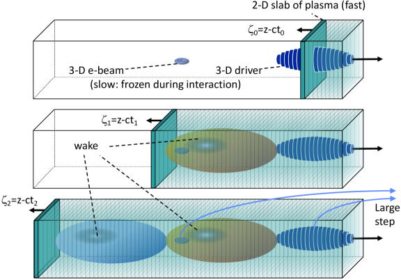
Assuming the driver at a given time and position, its high rigidity enables the approximation that it is quasi-static during the time that it takes for traversing a transverse slice of the plasma (assumed to be unperturbed by the driver ahead of it). The response of the plasma can thus be computed by following the evolution of the plasma slice as the driver propagates through it (See Fig. 24). The reconstruction of the longitudinal and transverse structure of the wake from the succession of transverse slices gives the full electric and magnetic field map for evolving the beam momenta and positions on a time scale that is commensurate with its rigidity.
Most formulations use the speed-of-light frame, defined as , to follow the evolution of the plasma slices. Assuming a slice initialized ahead of the driver, the evolution of the plasma particles inside the slice is given by:
| (59) | |||||
| (60) |
The plasma charge and current densities are computed by accumulating the contributions of each plasma macro-particle , corrected by the time taken by the particle to cross an interval of :
| (61) | |||||
| (62) |
In contrast, the evolution of a charged particle driver or witness beam (assumed to propagate near the speed of light), is given using the standard equations of motion:
| (63) | |||||
| (64) |
while their contributions to the charge and current densities are
| (65) | |||||
| (66) |
The electric and magnetic fields are obtained by either solving the equations of the scalar and vector potentials in the Coulomb or Lorentz gauge [13, 14] or directly the Maxwell’s equations [87, 88, 89, 90] which, under the quasi-static assumption
| (67) |
become
| (68) | |||
| (69) | |||
| (70) | |||
| (71) | |||
| (72) | |||
| (73) |
The set of equations on the potentials or the fields can then be rearranged in a set of 2-D Poisson-like equations that are solved iteratively with the particle motion equations. Unlike the Particle-In-Cell method, there is no single way of marching the set of equations together and the reader should refer to the descriptions of implementations in the various codes for more specific details [13, 14, 87, 88, 89, 90].
Appendix B The Ponderomotive Guiding Center approximation
For laser pulses with envelopes that are long compared to the laser oscillations, it is advantageous to average over the fast laser oscillations and solve the laser evolution with an envelope equation [13, 91, 14, 16, 92]. Assuming a laser pulse in the form of an envelope modulating a plane wave traveling at the speed of light,
| (74) |
the average response of a plasma to the fast laser oscillations can be described by a ponderomotive force that inserts into a modified equation of motion:
| (75) |
with
| (76) |
| (77) |
while the more complete envelope equation
| (78) |
that retains the second time derivative is solved in the code INF&RNO [92]. The latter equation is more exact, enabling the accurate simulation of the laser depletion into strongly depleted stages. As noted in [92], in order to avoid numerical inaccuracies, or having to grid the simulation very finely in the longitudinal direction, it is advantageous to use the polar representation of the laser complex field, namely , rather than the more common Cartesian splitting between the real and imaginary parts . As it turns out, the functions and are much smoother functions with respect to than and , which both exhibit very short wavelength oscillations in , leading to more accurate numerical differentiation along of the polar representation at a given longitudinal resolution.
Appendix C Electromagnetic PSATD PIC algorithm in a Galilean frame
In the Galilean coordinates , the equations of particle motion and the Maxwell equations take the form
| (79a) | ||||
| (79b) | ||||
| (79c) | ||||
| (79d) | ||||
where denotes a spatial derivative with respect to the Galilean coordinates .
Integrating these equations from to results in the following update equations (see [78] for the details of the derivation):
| (80a) | ||||
| (80b) | ||||
where we used the short-hand notations , as well as:
| (81a) | |||
| (81b) | |||
| (81c) | |||
| (81d) | |||