Controlling the spread of
COVID-19 on college campuses
Abstract
This research was done during the DOMath program at Duke University from May 18 to July 10, 2020. At the time, Duke and other universities across the country were wrestling with the question of how to safely welcome students back to campus in the Fall. Because of this, our project focused on using mathematical models to evaluate strategies to suppress the spread of the virus on campus, specifically in dorms and in classrooms. For dorms, we show that giving students single rooms rather than double rooms can substantially reduce virus spread. For classrooms, we show that moving classes with size above some cutoff online can make the basic reproduction number , preventing a wide spread epidemic. The cutoff will depend on the contagiousness of the disease in classrooms.
1 Introduction
As most readers know, the COVID-19 pandemic began in China in December 2019, then slowly spread around the world. Among its impacts on the US are changes to the education system. After Spring Break 2020, many colleges sent students home and switched to remote learning. During the summer, the big question became what to do in the fall. Colleges across the US have moved classes online, restricted the number of students on campus, and have modified semester schedules to run from mid-August to Thanksgiving with no breaks. To further control the spread of the virus on campus, they have made dining halls take-out only and reconfigured public spaces to encourage social distancing. In addition, there will be daily symptom reporting, increased testing, as well as quarantine and contact tracing for infected individuals.
In this paper we will consider two methods to suppress the spread of the virus. In Section 2, we ask the question: How much would spread be reduced if all students in dorms have single rooms? This is a significant issue for Duke because undergraduates are required to live on campus three of their four years, so at any time more than 80% live in dorms. By using a generalization of the household model [1], we show that the reduction can be substantial.
In Section 3, we turn our attention to classrooms and ask a two part question inspired by Gressman and Peck [2], who analyzed a complex stochastic agent based model to determine the impact of having large classes be online-only. The first part is: How does the distribution of class sizes affect virus spread? To approach this question, we considered two scenarios for a college that has students, each taking classes. In Scenario 1, all classes have size . In Scenario , 1/4 of the classes have size 60, and 3/4 have size 20. By calculating the maximum eigenvalue of the matrix that governs the spread in the second case, we show that the basic reproduction number is 48% larger in scenario 2 due to increased spread in larger classes.
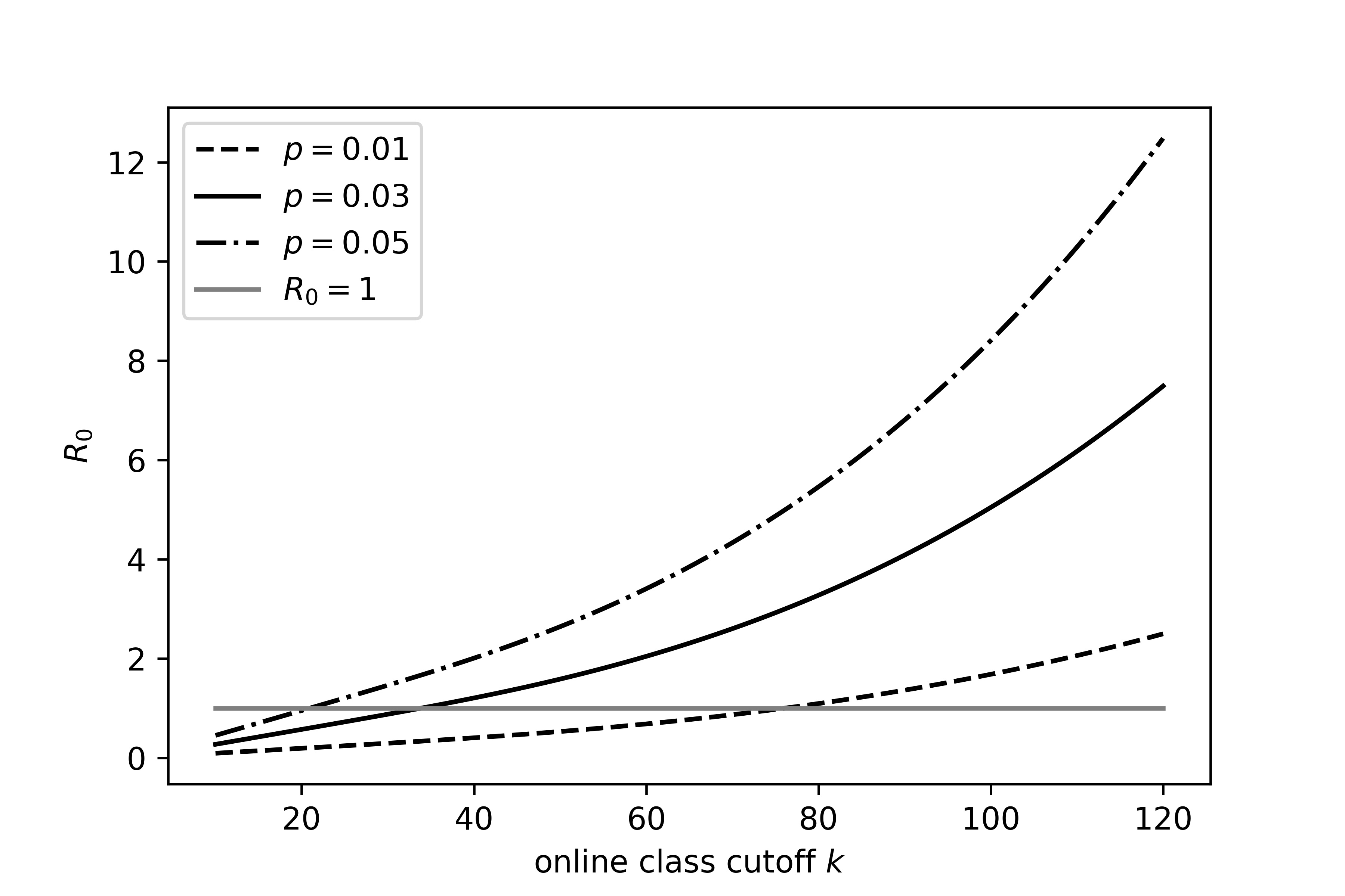
Knowing that larger classes promote virus spread, it is natural to move classes above a certain threshold online. Thus, the second question we ask in Section 3 is: Where should the threshold be for moving classes online? To address this question, we consider a scenario where 2405 students take three classes each and there is one class of each size from through . This is not a very realistic situation but it does allow us to investigate a wide range of cutoffs. We find that the threshold for moving classes online to reduce the basic reproduction number and hence stop the spread of the epidemic depends on the basic infection probability p in the model. For the values we investigate, the threshold can be as large as 70 or as small as 30.
2 Household model and college dorms
The question that motivates this section is: To what extent would the spread of COVID-19 on the Duke campus be reduced if all students had single rooms? To answer this question, we will use results that have been developed for the household model. See [1] and references therein. The household model improves slightly on a homogeneous mixing model by partitioning the population into multiple households with the probability of infecting an individual being larger for individuals in the same household.
We will review the necessary theory on the household model in Section 2.1. In Section 2.2, we examine the case where all students have single rooms by viewing dorms as households and applying the household model. In Section 2.3, where we examine double rooms, we still view dorms as households, but generalize our approach on computing the dynamics within a household.
2.1 Household model
Let the population of size be split into households of size . For simplicity, we consider the case of fixed infection time. Let be the probability an individual infects individual who is another member of the same house. Let be the probability of infecting individual who is not in the same house as individual . is used to denote household, and is used to denote global.
Step 1: Connect each pair of individuals in the same house with probability .
Let be the probability an individual belongs to a cluster of size . Let be the mean cluster size, and let be the generating function of the cluster size.
Step 2: Make long distance connections between individuals in different households with probability .
The number of long distance infections caused by one person is Poisson() if is large. The generating function of is .
From step 1 and 2, we see that
To compute the generating function, we recall that if are independent with generating functions and , then has generating function . This implies that the generating function of the number of individuals infected by a cluster of size is and hence that the number of individuals infected by the cluster of a randomly chosen individual is
A well-known result for branching processes implies that the probability of a large epidemic is the solution of
| (1) |
When we apply the household model to our dorm models by viewing a dorm as a household, will vary between models since the choice of single or double rooms results in a slightly altered local spread within a dorm. On the other hand, since the global spread of the infection is unaffected by room size, will be the same for the two dorm scenarios.
2.2 Single Rooms
In adapting the household model to the spread of infection in a college dorm, will instead be written as , since we are concerned with a dorm rather than a household. Similarly, will instead be written as , with the superscript 1 indicating single rooms.
We first compute . Consider dorms with single rooms, where population size . If is large, e.g., 120 is the size of a typical freshman dorm at Duke, then the total number of individuals infected in one dorm as a result of one infected is the total progeny of a branching process. The branching process will have the offspring distribution Poisson(), where . We assume so that the mean of the total progeny is
| (2) |
Each individual infected in the dorm infects an average of individuals outside the dorm so the basic reproduction number is
| (3) |
Now, we solve for . Breaking things down according to the number of individuals directly infected by the first individual, the generating function of the size of the epidemic within the dorm caused by one infected is
| (4) |
where , the generating function of the spread of the infection within the dorm. One method for solving (4) is through iteration. We start with , which corresponds to 1 individual in generation 0, and then iterate
| (5) |
is the generating function of the number of individuals infected in the first generations of the process, so , a solution of the recursion.
In the case of single rooms, an explicit solution for can be found by taking the derivative of equation (4) to get the differential equation
with the boundary condition . It is well known that the solution to the differential equation is
| (6) |
where is the Lambert function which is defined by .

By (1), the probability of a large epidemic is the largest solution of
| (7) |
This can be further simplified. Plugging in yields
Multiplying through by , then applying to both sides gives
Recalling that and simplifying, we obtain
which is the survival probability for a branching process with a Poisson() distribution. We do not have an intuitive understanding of why this is true.
2.3 Double Rooms
Suppose now that we have dorms with double rooms, so that . For the sake of comparison, we let the number of people in a dorm be the same, regardless of whether they have only single rooms or only double rooms, i.e., . Let be the probability of infecting your roommate, and be the probability of infecting an individual within your dorm. To find the analogue of in this scenario, we think of a generation as having a first step where the ancestor splits into two with probability , stays 1 with probability and then a second step in which long range connections are formed within the dorm. The offspring distribution is now a mixture of two Poissons:
The mean number of infections in one generation, , will be the sum of the means of the two Poisson distributions so .
Imitating calculations in Section 2.2, if , the mean of the total progeny of the branching process is
| (8) |
and the basic reproduction number is
| (9) |
To compute , the analogue of for the double room scenario, we note that the generating function of the number of infections in one generation is
so satisfies
| (10) |
can then be solved with the iteration method described in Section 2.2.
Having computed we can compute the probability of a large epidemic as in the previous case by numerically solving
| (11) |
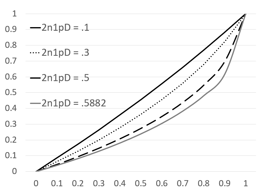
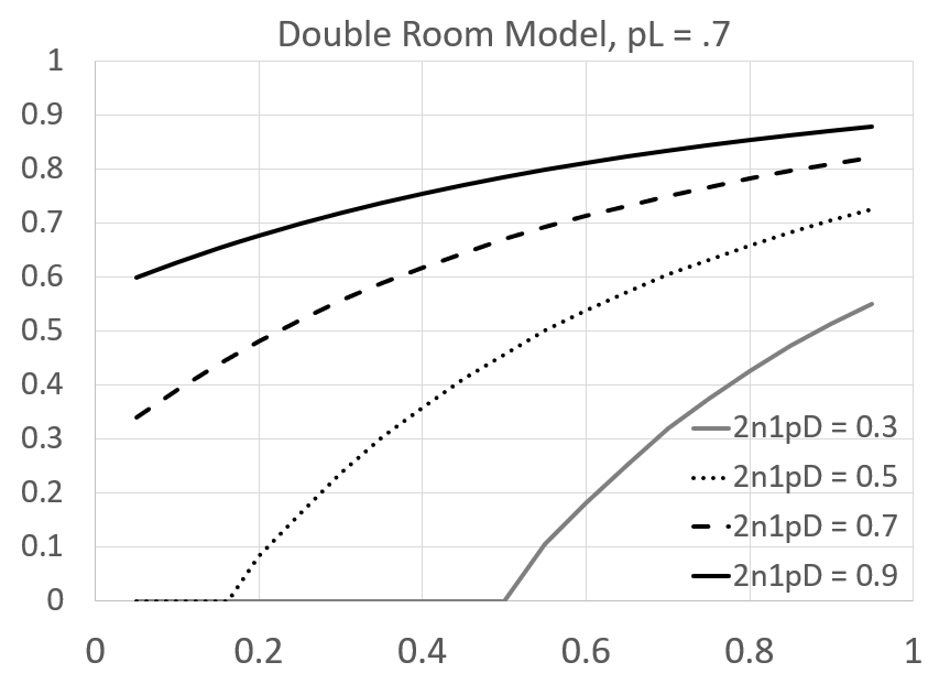
A comparison of the epidemic probabilities for double-room and single-room dorms is given in Figure 3. Note that in the double-room situation when or 0.9, there is a positive probability of a large epidemic within a single dorm, so the curves are positive when . When or 0.5, needs to exceed a positive threshold for there to be an epidemic in a university with double-room dorms, but those thresholds are higher when there are only single-room dorm.

3 Spread of infection in college classes
This section addresses two questions. The first asks how different class size distributions affect pandemic spread. The second asks whether taking classes above a certain size online can prevent outbreaks.
To address these questions, we consider some simplified models in which each student takes three classes. The situation can be described by a graph in which there are students and classes with sizes , and there is an edge from each student to the three classes they are enrolled in. Each classroom is assumed to be homogeneously mixing. To formulate the dynamics, we say that the three class members that correspond to one student are their alter egos.
An individual that is infected in class at time, adds his two alter egos (his presence in other classes) to the infected population at time and then infections at time are produced. None of the infecteds from time are present at time .
3.1 Equal class sizes reduce spread
To show that class sizes impact spread, we compare two scenarios for a college with that each take three classes.
Scenario 1. 100 classes of size 30. An individual infected in class at time 0 will produce a Poisson() number of new infected individuals in class at time 1. His two alter egos are equally likely to be in classes 2-100, and each alter ego will produce Poisson() infecteds in whichever class they are in. So if is the mean number of infecteds in class at time 1 from a single infected person in class , then
From this we see that an infected at time 0 produces an average of infecteds at time 1 so
| (12) |
Scenario 2. 25 classes of size 60 () and 75 of size 20 (). Let be the expected number of infections in class caused by one infected student in . and represent that sizes of class i and j respectively. In this scenario, the probability that an individual in class has an alter ego in a different class is , where is the size of class . The comes from alter egos. Thus, we have
Since the eigenvector associated with the maximum eigenvalue will have for and for , the eigenvalue problem for the matrix can be reduced to the eigenvalue problem for the matrix with entries
Solving a quadratic shows that this matrix has eigenvalues and . Thus,
| (13) |
This value is 48% larger than the for scenario 1, and suggests that larger classes increase virus transmission.
3.2 Stochastic model for scenarios 1 and 2
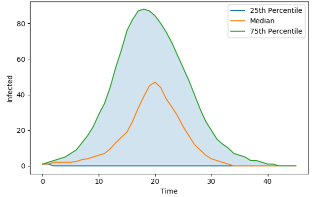
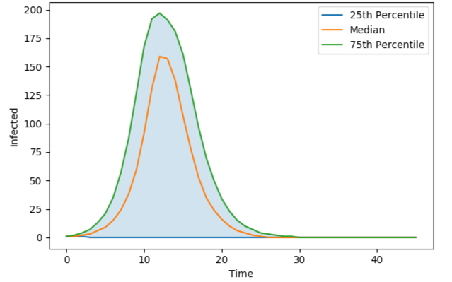
For a more detailed look at the two scenarios, we turn to a stochastic model. As in the previous section the model takes place in discrete time. Each time step is roughly one class meeting, so that two time steps are roughly equivalent to a week in real time. An infected person in a class infects each other individual with probability and has a 0.5 probability of entering quarantine. Using (12) we see that in scenario 1. (13) implies that . is a commonly used value for an uncontrolled COVID-19 epidemic. Figures 4 and 5 confirm that Scenario 2 is worse than Scenario 1.
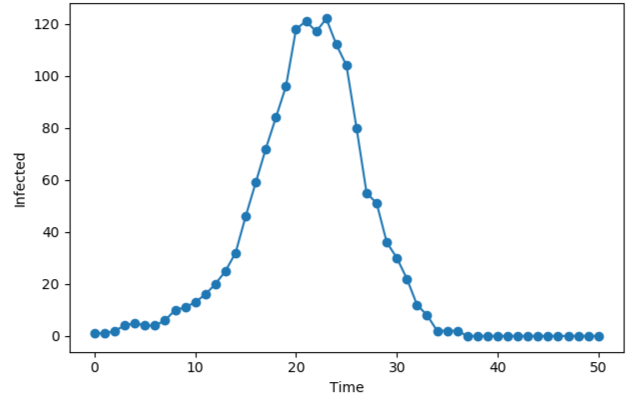
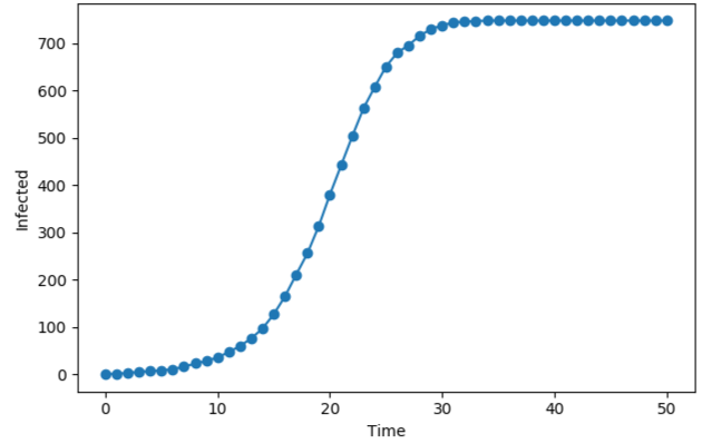
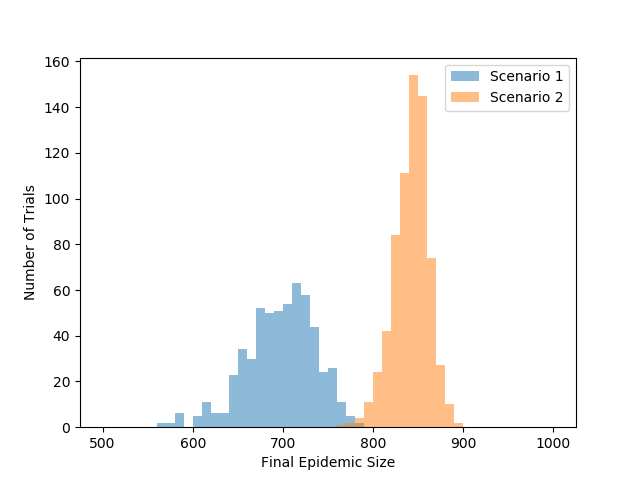
The next figure compares the equal class size and 60–20 scenarios. In both scenarios, the outbreak generally grows out of control within a few weeks and infects the majority of students. In Scenario 2, the outbreaks tend to develop faster, have a higher peak, and vary less in size and dynamics. Scenario 2 also produces a higher probability a large outbreak will occur from one individual, and larger final epidemic sizes. Thus, it is clear that the presence of larger classes, even if average class size remains the same, increases the risks for students on campus.
3.3 Moving Classes Online
In this section, we consider the effects of moving classes above a given size online. To do so, we consider a university with 111 classes, one each of sizes ranging from 10, 11… 120. The total class size is and there are students. To begin, we first consider when all classes are in person.
Following the calculations for scenario 2 in Section 3.1, we see that the average number fo people infected in classroom by an infected individual in classroom is
Similar to the previous scenarios in this section, we find the largest eigenvalue of the above matrix to determine . Although we were unable to find the eigenvalue analytically, we used Python to determine that
When , .
We now look at the situation where the university moves all of its classes of size . Viruses can’t spread through online classes, we have
The other values of remain unchanged. The change in depending on and various can be seen in Figure 7, which makes clear that establishing a cutoff can sharply reduce virus spread through classes. Although Gressman and Peck suggested a cutoff of based on their stochastic simulations for spread in universities [2], our results in Figure 7 suggest that the optimal cutoff depends largely on . For sufficiently small , even cutoffs as high as can be effective.
References
- [1] Ball, F., Mollison, D., and Scalia-Tomba, G. (1997) Epidemics with two levels of mixing. Annals Applied Probability. 7, 46–89
- [2] Gressman, P.T., and Peck, J.R. (2020) Simulating COVID-19 in a University Environment arXiv:2006.03175