Forward and inverse reinforcement learning sharing network weights and hyperparameters

Abstract

This paper proposes model-free imitation learning named Entropy-Regularized Imitation Learning (ERIL) that minimizes the reverse Kullback-Leibler (KL) divergence. ERIL combines forward and inverse reinforcement learning (RL) under the framework of an entropy-regularized Markov decision process. An inverse RL step computes the log-ratio between two distributions by evaluating two binary discriminators. The first discriminator distinguishes the state generated by the forward RL step from the expert’s state. The second discriminator, which is structured by the theory of entropy regularization, distinguishes the state-action-next-state tuples generated by the learner from the expert ones. One notable feature is that the second discriminator shares hyperparameters with the forward RL, which can be used to control the discriminator’s ability. A forward RL step minimizes the reverse KL estimated by the inverse RL step. We show that minimizing the reverse KL divergence is equivalent to finding an optimal policy. Our experimental results on MuJoCo-simulated environments and vision-based reaching tasks with a robotic arm show that ERIL is more sample-efficient than the baseline methods. We apply the method to human behaviors that perform a pole-balancing task and describe how the estimated reward functions show how every subject achieves her goal.

1 Introduction

Reinforcement Learning (RL) is a computational framework for investigating the decision-making processes of both biological and artificial systems that can learn an optimal policy by interacting with an environment (Sutton and Barto, 1998; Doya, 2007; Kober et al., 2013). Modern RL algorithms have achieved remarkable performance in playing Atari games (Mnih et al., 2015), Go (Silver et al., 2017), Dota 2 (OpenAI et al., 2019), and Starcraft II (Vinyals et al., 2019). They have also been successfully applied to dexterous manipulation tasks (OpenAI et al., 2019), folding a T-shirt (Tsurumine et al., 2019), quadruped locomotion (Haarnoja et al., 2018), the optimal state feedback control of nonaffine nonlinear systems (Wang and Qiao, 2019), and non-zero-sum game output regulation problems (Odekunle et al., 2020). However, one critical open question in RL is designing and preparing an appropriate reward function for a given task. Although it is easy to design a sparse reward function that gives a positive reward when a task is accomplished and zero otherwise, such an approach complicates finding an optimal policy due to prohibitive learning times. On the other hand, we can accelerate the learning speed with a complicated function that generally gives a non-zero reward signal. However, optimized behaviors often deviate from an experimenter’s intention if the reward function is too complicated (Doya and Uchibe, 2005).

In some situations, it is easier to prepare examples of a desired behavior provided by an expert than handcrafting an appropriate reward function. Behavior Cloning (BC) is a straightforward approach in imitation learning formulated as supervised learning. BC minimizes the forward Kullback-Leibler (KL) divergence, which is known as moment projection (M-projection). Forward KL is the expectation of the log-likelihood ratio under expert distribution. Although BC requires no interaction with the environment, it suffers from a state covariate shift problem: small errors in actions introduce the learner to unseen states that are not included in the training dataset (Ross et al., 2011). Also, BC shows poor performance if the model is misspecified because minimizing the forward KL has a mode-covering property. To overcome the covariate shift problem, several inverse RL (Ng and Russell, 2000) and apprenticeship learning (Abbeel and Ng, 2004) methods have been proposed to retrieve a reward function from expert behaviors and implement imitation learning. Currently available applications include a probabilistic driver route prediction system (Vogel et al., 2012; Liu et al., 2013), modeling risk anticipation and defensive driving (Shimosaka et al., 2014), investigating human behaviors in table tennis (Muelling et al., 2014), robot navigation tasks (Kretzschmar et al., 2016; Xia and El Kamel, 2016), analyzing animal behaviors (Ashida et al., 2019; Hirakawa et al., 2018; Yamaguchi et al., 2018), and parser training (Neu and Szepesvári, 2009). A recent functional magnetic resonance imaging (fMRI) study suggests that the anterior part of the dorsomedial prefrontal cortex (dmPFC) is likely to encode the inverse reinforcement learning algorithm (Collette et al., 2017). Combining inverse RL with a standard RL is a promising approach to find an optimal policy from expert demonstrations. Hereafter, we use the term “forward” reinforcement learning to clarify the difference.

Recently, some works (Fu et al., 2018; Ho and Ermon, 2016) have connected forward and inverse RL and Generative Adversarial Networks (GANs) (Goodfellow et al., 2014), which exhibited remarkable success in image generation, video prediction, and machine translation domains. In this view, inverse RL is interpreted as a GAN discriminator whose goal is to determine whether experiences are drawn from an expert or generated by a forward RL step. The GAN generator is implemented by a forward RL step and creates experiences that are indistinguishable by an inverse RL. Generative Adversarial Imitation Learning (GAIL) (Ho and Ermon, 2016) showed that the iterative process of forward and inverse RL produces policies that outperformed BC. However, GAIL minimizes the Jensen-Shannon divergence, which has a similar forward KL property. In addition, GAIL is sample-inefficient because an on-policy RL algorithm used in the forward RL step simply trains a policy from a reward calculated by the inverse RL step. To improve the sample efficiency in the forward RL step, Jena et al. (2020) added BC loss to the loss of the GAIL generator. Kinose and Taniguchi (2020) integrated the GAIL discriminator with reinforcement learning, in which the policy is trained with both the original reward and additional rewards calculated by the discriminator. However, their approaches remain sample-inefficient. Utilizing the result of the inverse RL step to the forward RL step and vice versa is difficult because the discriminator’s structure is designed independently from the generator.

To further improve the sample efficiency, this paper proposes a model-free imitation learning algorithm named Entropy-Regularized Imitation Learning (ERIL), which minimizes the information projection or the I-projection, which is also known as the reverse KL divergence between two probability distributions induced by a learner and an expert. A reverse KL, which is the expectation of the log-likelihood ratio under the learner’s distribution, has a mode-seeking property that focuses on the distribution mode that the policy can represent. A reverse KL is more appropriate than a forward KL when the policy is misspecified. Unfortunately, reverse KL divergence cannot be computed because the expert distribution is unknown. Our idea applies the density ratio trick (Sugiyama et al., 2012) to evaluate the log-ratio between two distributions from samples drawn from them. In addition, we exploit the framework of the entropy-regularized Markov Decision Process (MDP), where the reward function is augmented by the differential entropy of a learner’s policy and the KL divergence between the learner and expert policies. Consequently, the log-ratio can be computed by training two binary discriminators. One is a state-only discriminator, which distinguishes the state generated by the learner from the expert’s state. The second discriminator, which is a function of a tuple of a state, an action, and the next state, also distinguishes between the experiences of learners and experts. The second discriminator is represented by reward, a state value function, and the log-ratio of the first discriminator. We show that Adversarial Inverse Reinforcement Learning (AIRL) (Fu et al., 2018) and Logistic Regression-based Inverse RL (LogReg-IRL) (Uchibe and Doya, 2014; Uchibe, 2018) discriminators are a special case of an ERIL. The loss function is essentially identical as that of GAN for training discriminators, which are efficiently trained by logistic regression.

After evaluating the log-ratio, the forward RL in ERIL minimizes the estimated I-projection. We show that its minimization is equivalent to maximizing the entropy-regularized reward. Consequently, the forward RL algorithm is implemented by off-policy reinforcement learning that resembles Dynamic Policy Programming (Azar et al., 2012), Soft Actor-Critic (SAC) (Haarnoja et al., 2018), and conservative value iteration (Kozuno et al., 2019). In the forward RL step, the state value, the state-action value, and the stochastic policy are trained by the actor-critic algorithm, and the reward function estimated by the inverse RL step is fixed. This step allows the learner to generalize the expert policy to unseen states that are not included in the demonstrations.

We experimented with the MuJoCo benchmark tasks (Todorov et al., 2012) in the OpenAI gym (Brockman et al., 2016). Our experimental results demonstrate that ERIL resembles some modern imitation learning algorithms in terms of the number of trajectories from expert data and outperformed sample efficiency in terms of the number of trajectories in the forward RL step. Ablation studies show that entropy regularization plays a critical role in improving sample efficiency. Next we conducted a vision-based target-reaching task with a manipulator in three-dimensional space and demonstrated that using two discriminators is vital when the learner’s initial state distribution differs from the expert one. Then we applied ERIL to human behaviors for performing a pole-balancing task. Since the actions of human subjects are not observable, the task is an example of realistic situations. ERIL recovers the subjects’ policies better than the baselines. We also showed that the estimated reward functions show how every subject achieved her goal.

The following are the main contributions of our paper: (1) We proposed a structured discriminator with hyperparameters derived from entropy-regularized reinforcement learning. (2) The hyperparameters, which are shared between forward and inverse RL, can be used to control the discriminator’s ability. (3) The state value function is trained by both forward and inverse RL, which improves the sample efficiency in terms of the number of environmental interactions.

2 Related Work

2.1 Regularization in RL

The role of regularization is to prevent overfitting and to encourage generalization. Many regularization methods have been proposed from various aspects, such as dropout (Liu et al., 2021), temporal difference error (Parisi et al., 2019), value function difference (Ohnishi et al., 2019), and manifold regularization for feature representation learning (Li et al., 2018). Amit et al. (2020) investigated the property of a discount factor as a regularizer.

The most widely used regularization method is entropy regularization (Ziebart et al., 2008; Belousov and Peters, 2019). It supports exploration by favoring more stochastic policies (Haarnoja et al., 2018) and smoothens the optimization landscape (Ahmed et al., 2019). The advantage of entropy regularization in inverse RL is its robustness against noisy and stochastic demonstrations because an optimal policy becomes stochastic.

2.2 Behavior cloning

BC directly maximizes the log-likelihood of an expert action. Pomerleau (1989) achieved an Autonomous Land Vehicle In a Neural Network (ALVINN), which is a potential precursor of autonomous driving cars. ALVINN’s policy is implemented by a 3-layer neural network and learns mappings from video and range finder inputs to steering directions by supervised learning. However, ALVINN suffers from the covariate shift problem. To reduce covariate shift, Ross et al. (2011) proposed an iterative method called Dataset Aggregation (DAGGER), where the learner runs its policy while the expert provides the correct action for the states visited by the learner. Laskey et al. (2017) proposed Disturbances for Augmented Robot Trajectories (DART), which collects expert datasets with injected noise.

It is often difficult to provide such expert data as state-action pairs in such realistic situations as analyzing animal behaviors and learning from videos. Torabi et al. (2018) studied a situation in which expert action is unavailable and proposed Behavioral Cloning from Observation (BCO) that estimates actions from an inverse dynamics model. Soft Q Imitation Learning (SQIL) (Reddy et al., 2020) is a BC with a regularization term that penalizes large squared soft Bellman error. SQIL is implemented by SAC, which assigns the reward of the expert data to 1 and the generated data to 0. SQIL can learn from both the expert and learner’s samples because SAC is an off-policy algorithm.

2.3 Generative adversarial imitation learning

GAIL (Ho and Ermon, 2016), which is a very popular imitation learning algorithm, formulates the objectives of imitation learning as GAN training objectives. Its discriminator differentiates between generated state-action pairs and those of experts, and the generator acts as a forward reinforcement learning algorithm to maximize the sum of rewards computed by the discriminator. There are several extensions of GAN. AIRL (Fu et al., 2018) used an optimal discriminator whose expert distribution was approximated by a disentangled reward function. A similar, independently proposed discriminator (Uchibe and Doya, 2014; Uchibe, 2018) was derived from the framework of entropy-regularized reinforcement learning and density ratio estimation. AIRL experimentally showed that the learned reward function can be transferred to new, unseen environments. Situated GAIL (Kobayashi et al., 2019) extended GAIL to learn multiple reward functions and multiple policies by introducing a task variable to both the discriminator and the generator.

As discussed in the previous section, expert action is not always available. IRLGAN (Henderson et al., 2018) is a special GAN case where the discriminator is given as a state function. Torabi et al. (2019) proposed Generative Adversarial Imitation from Observation (GAIfO) whose functions are characterized by state transitions. Sun and Ma (2014) proposed Action Guided Adversarial Imitation Learning (AGAIL) that can deal with expert demonstrations with incomplete action sequences. AGAIL uses mutual information between expert and generated actions as an additional regularizer for training objectives.

To reduce the number of interactions in the forward RL step, Blondé and Kalousis (2019) proposed Sample-efficient Adversarial Mimic (SAM), which adopts an off-policy method called the Deep Deterministic Policy Gradients (DDPG) algorithm (Lillicrap et al., 2016). SAM maintains three different neural networks, which approximate a reward function, a state-action value function, and a policy. The reward function is estimated in the same way as in GAN, and the state-action value function and the policy are trained by DDPG. Kostrikov et al. (2019) showed that GAIL’s reward function is biased and that the absorbing states are not treated appropriately. They proposed a preprocessing technique for expert data before learning and developed the Discriminator Actor-Critic (DAC) algorithm. DAC utilizes the Twin Delayed Deep Deterministic policy gradient (TD3) algorithm (Fujimoto et al., 2018), which is an extension of DDPG. Sasaki et al. (2019) exploited the Bellman equation to represent a reward function, and a reward’s exponential transformation is trained as a kind of discriminator. They improved the policy using an off-policy actor-critic (Degris et al., 2012). Zuo et al. (2020) proposed a Deterministic GAIL that adopts the modified DDPG algorithm that incorporates the behavior cloning loss in the forward RL step. Discriminator Soft Actor-Critic (Nishio et al., 2020) extended SQIL by estimating the reward function by an AIRL-like discriminator. Ghasemipour et al. (2019) and Ke et al. (2020) described the relationship between several imitation learning algorithms from the viewpoint of objective functions. Since our study focuses on sample efficiency with respect to the number of interactions with the environment, the most related works are SAM, DAC, and Sasaki’s method. We compared our method with these three methods in the experiments.

3 Preliminaries

3.1 Markov decision process

Here we briefly introduce MDP for a discrete-time domain. Let $\mathcal{X}$ and $\mathcal{U}$ be continuous or discrete state and action spaces. At time step $t$, a learning agent observes environmental current state $\bm{x}_{t}\in\mathcal{X}$ and executes action $\bm{u}_{t}\in\mathcal{U}$ sampled from stochastic policy $\pi(\bm{u}_{t}\mid\bm{x}_{t})$. Consequently, the learning agent receives from the environment immediate reward $\tilde{r}(\bm{x}_{t},\bm{u}_{t})$, which is an arbitrary bounded function that evaluates the goodness of action $\bm{u}_{t}$ at state $\bm{x}_{t}$. The environment shifts to next state $\bm{x}_{t}^{\prime}=\bm{x}_{t+1}\in\mathcal{X}$ according to state transition probability $p_{T}(\bm{x}_{t}^{\prime}\mid\bm{x}_{t},\bm{u}_{t})$.

Forward reinforcement learning’s goal is to construct optimal policy $\pi(\bm{u}\mid\bm{x})$ that maximizes the given objective function. Among several available objective functions, the most widely used is a discounted sum of rewards:

$$V(\bm{x})\triangleq\mathbb{E}\left[\sum_{t=0}^{\infty}\gamma^{t}\tilde{r}(\bm{x}_{t},\bm{u}_{t})\mid\bm{x}_{0}=\bm{x}\right],$$

where $\gamma\in[0,1)$ is called the discount factor. The optimal state value function for the discounted reward setting satisfies the following Bellman optimality equation:

$$V(\bm{x})=\max_{\bm{u}}\left[\tilde{r}(\bm{x},\bm{u})+\gamma\mathbb{E}_{\bm{x}^{\prime}\sim p_{T}(\cdot\mid\bm{x},\bm{u})}\left[V(\bm{x}^{\prime})\right]\right],$$ (1)

where $\mathbb{E}_{p}[\cdot]$ hereafter denotes the expectation with respect to $p$. The state-action value function for the discounted reward setting is also defined:

$$Q(\bm{x},\bm{u})=\tilde{r}(\bm{x},\bm{u})+\gamma\mathbb{E}_{\bm{x}^{\prime}\sim p_{T}(\cdot\mid\bm{x},\bm{u})}\left[V(\bm{x}^{\prime})\right].$$

Eq. (1), which is nonlinear due to the max operator, usually struggles to find an action that maximizes its right hand side.

3.2 Entropy-regularized Markov decision process

Next we consider entropy-regularized MDP (Azar et al., 2012; Haarnoja et al., 2018; Kozuno et al., 2019; Ziebart et al., 2008), in which the reward function is regularized by the following form:

$$\tilde{r}(\bm{x},\bm{u})=r(\bm{x},\bm{u})+\frac{1}{\kappa}\mathcal{H}(\pi(\cdot\mid\bm{x}))-\frac{1}{\eta}\mathrm{KL}(\pi(\cdot\mid\bm{x})\parallel b(\cdot\mid\bm{x})),$$ (2)

where $r(\bm{x},\bm{u})$ is a standard reward function that is unknown in the inverse RL setting. $\kappa$ and $\eta$ are the positive hyperparameters determined by the experimenter, $\mathcal{H}(\pi(\cdot\mid\bm{x}))$ is the (differential) entropy of policy $\pi(\bm{u}\mid\bm{x})$, and $\mathrm{KL}(\pi(\cdot\mid\bm{x})\parallel b(\cdot\mid\bm{x}))$ is the relative entropy, which is also known as the Kullback-Leibler (KL) divergence between $\pi(\bm{u}\mid\bm{x})$ and baseline policy $b(\bm{u}\mid\bm{x})$. When the reward function is regularized by the entropy functions (2), we can analytically maximize the right hand side of Eq. (1) by a method using Lagrange multipliers. Consequently, the optimal state value function can be represented:

$$V(\bm{x})=\frac{1}{\beta}\ln\int\exp\left(\beta Q(\bm{x},\bm{u})\right)\mathrm{d}\bm{u},$$ (3)

where $\beta$ is a positive hyperparameter defined by

$$\beta\triangleq\frac{\kappa\eta}{\kappa+\eta},$$

and $Q(\bm{x},\bm{u})$ is the optimal soft state-action value function:

$$Q(\bm{x},\bm{u})=r(\bm{x},\bm{u})+\frac{1}{\eta}\ln b(\bm{u}\mid\bm{x})+\gamma\mathbb{E}_{\bm{x}^{\prime}\sim p_{T}(\cdot\mid\bm{x},\bm{u})}\left[V(\bm{x}^{\prime})\right].$$ (4)

When the action is discrete, the right hand side of Eq. (3) is a log-sum-exp function, also known as a softmax function. The corresponding optimal policy is given:

$$\pi(\bm{u}\mid\bm{x})=\frac{\exp(\beta Q(\bm{x},\bm{u}))}{\exp(\beta V(\bm{x}))},$$ (5)

where $\exp(\beta V(\bm{x}))$ represents a normalizing constant of $\pi(\bm{u}\mid\bm{x})$.

For later reference, the update rules are described here. The soft state-action value function is trained to minimize the soft Bellman residual. The soft state value function is trained to minimize the squared residual error derived from Eq. (5). The policy is improved by directly minimizing the expected KL divergence in Eq. (5):

$$J_{\mathrm{ER}}(\bm{w}_{\pi})=\mathbb{E}_{\bm{x}\sim p(\bm{x})}\left[\mathrm{KL}\left(\pi(\cdot\mid\bm{x})\parallel\frac{\exp(\beta Q(\bm{x},\cdot))}{\exp(\beta V(\bm{x}))}\right)\right].$$

The derivative of the KL divergence is given by

$$\nabla\mathrm{KL}=\mathbb{E}_{\bm{u}\sim\pi(\cdot\mid\bm{x})}\left[\nabla_{\bm{w}_{\pi}}\ln\pi(\cdot\mid\bm{x})\left[\ln\pi(\cdot\mid\bm{x})-\beta(Q(\bm{x},\cdot)-V(\bm{x}))+B(\bm{x})\right]\right],$$ (6)

where $B(\bm{x})$ is a baseline function that does not change the gradient (Peters and Schaal, 2008) and is often used to reduce the variance of the gradient estimation.

3.3 Generative adversarial networks

GANs are a class of neural networks that can approximate probability distribution based on a game theoretic scenario (Goodfellow et al., 2014). Standard GANs consist of a generator and a discriminator. Suppose that $p^{E}(\bm{z})$ and $p^{L}(\bm{z})$ denote the probability distributions over data $\bm{z}$ of the expert and a generator. A discriminator, which is a function that distinguishes samples from a generator and an expert, is denoted by $D(\bm{z})$ and minimizes the following negative log-likelihood (NLL):

$$J_{\mathrm{GAN}}^{(D)}=-\mathbb{E}_{\bm{z}\sim p^{L}}[\ln D(\bm{z})]-\mathbb{E}_{\bm{z}\sim p^{E}}[\ln(1-D(\bm{z}))].$$ (7)

The optimal discriminator has the following shape (Goodfellow et al., 2014):

$$D^{\ast}(\bm{z})=\frac{p^{L}(\bm{z})}{p^{L}(\bm{z})+p^{E}(\bm{z})}.$$ (8)

The generator minimizes $-J_{\mathrm{GAN}}^{(D)}$:

$$J_{\mathrm{GAN}}^{(G)}=\mathbb{E}_{\bm{z}\sim p^{L}}[\ln D(\bm{z})],$$ (9)

where the second term on the right hand side of Eq. (7) is removed because it is constant with respect to the generator. Recently, Prescribed GAN (PresGAN) introduced an entropy regularization term to $J_{\mathrm{GAN}}$ to mitigate mode collapse (Dieng et al., 2019).

GAIL (Ho and Ermon, 2016) is an extension of GANs for imitation learning, and its objective function is given by

$$J_{\mathrm{GAIL}}(\bm{w}_{G},\bm{w}_{D}) =-\mathbb{E}_{(\bm{x},\bm{u})\sim\pi^{L}}[\ln D(\bm{x},\bm{u})]-\mathbb{E}_{(\bm{x},\bm{u})\sim\pi^{E}}[\ln(1-D(\bm{x},\bm{u}))]$$

$$\qquad+\lambda_{\mathrm{GAIL}}\mathcal{H}(\pi^{L}),$$

where $\lambda_{\mathrm{GAIL}}$ is a positive hyperparameter. Adding the entropy term is key for an association with the entropy-regularized MDP. The objective function of the GAIL discriminator is essentially identical as that of the GAN discriminator, which updates its policy by Trust Region Policy Optimization (TRPO) (Schaul et al., 2015), where the reward function is defined by

$$r_{\mathrm{GAIL}}=-\ln D(\bm{x},\bm{u}).$$

AIRL (Fu et al., 2018) adopts a special structure for the discriminator:

$$D(\bm{x},\bm{u},\bm{x}^{\prime})=\frac{\pi^{L}(\bm{u}\mid\bm{x})}{\exp(f(\bm{x},\bm{u},\bm{x}^{\prime}))+\pi^{L}(\bm{u}\mid\bm{x})},$$ (10)

where $f(\bm{x},\bm{u},\bm{x}^{\prime})$ is defined using two state-dependent functions, $g(\bm{x})$ and $h(\bm{x})$:

$$f(\bm{x},\bm{u},\bm{x}^{\prime})\triangleq g(\bm{x})+\gamma h(\bm{x}^{\prime})-h(\bm{x}).$$ (11)

Note that the AIRL discriminator (10) has no hyperparameters. A similar discriminator was proposed (Uchibe and Doya, 2014; Uchibe, 2018). AIRL’s reward function is calculated:

$$r_{\mathrm{AIRL}} =-\ln D(\bm{x},\bm{u})+\ln(1-D(\bm{x},\bm{u}))$$

$$=f(\bm{x},\bm{u},\bm{x}^{\prime})-\ln\pi(\bm{u}\mid\bm{x}).$$ (12)

Note that $-\ln D$ and $\ln(1-D)$ are monotonically related.

3.4 Behavior cloning

BC is the most widely used type of imitation learning. It minimizes the “forward” KL divergence, which is also known as M-projection (Ghasemipour et al., 2019; Ke et al., 2020):

$$J_{\mathrm{BC}}(\bm{w}_{\pi})=\mathrm{KL}(\pi^{E}\parallel\pi^{L})=-\mathbb{E}_{\pi^{E}}\left[\ln\pi^{L}(\bm{u}\mid\bm{x})\right]+C,$$ (13)

where $\bm{w}_{\pi}$ is the policy parameter vector of $\pi^{L}(\bm{u}\mid\bm{x})$ and $C$ is a constant with respect to the policy parameter. Since BC does not need to interact with the environment, finding a policy that minimizes Eq. (13) is simply achieved by supervised learning. Unfortunately, it suffers from covariate shift between the learner and the expert (Ross et al., 2011).

4 Entropy-Regularized Imitation Learning

4.1 Objective function

To formally present our approach, we denote the expert’s policy as $\pi^{E}(\bm{u}\mid\bm{x})$ and the learner’s policy as $\pi^{L}(\bm{u}\mid\bm{x})$. Suppose a dataset of transitions generated by

$$\mathcal{D}^{E}=\{(\bm{x}_{i},\bm{u}_{i},\bm{x}_{i}^{\prime})\}_{i=1}^{N^{E}},\quad\bm{u}_{i}\sim\pi^{E}(\cdot\mid\bm{x}_{i}),\quad\bm{x}_{i}^{\prime}\sim p_{T}(\cdot\mid\bm{x}_{i},\bm{u}_{i}),$$

where $N^{E}$ is the number of transitions in the dataset. We consider two joint probability density functions, $\pi^{E}(\bm{x},\bm{u},\bm{x}^{\prime})$ and $\pi^{L}(\bm{x},\bm{u},\bm{x}^{\prime})$, where under a Markovian assumption, $\pi^{E}(\bm{x},\bm{u},\bm{x}^{\prime})$ is decomposed by

$$\pi^{E}(\bm{x},\bm{u},\bm{x}^{\prime})=p_{T}(\bm{x}^{\prime}\mid\bm{x},\bm{u})\pi^{E}(\bm{u}\mid\bm{x})\pi^{E}(\bm{x}),$$ (14)

and $\pi^{L}(\bm{x},\bm{u},\bm{x}^{\prime})$ can be decomposed in the same way.

ERIL minimizes the “reverse” KL divergence given by

$$J_{\mathrm{ERIL}}(\bm{w}_{\pi})=\mathrm{KL}(\pi^{L}\parallel\pi^{E}),$$ (15)

where the reverse KL divergence is often called information projection (I-projection), defined by

$$\mathrm{KL}(\pi^{L}\parallel\pi^{E})=\mathbb{E}_{\pi^{L}}\left[\ln\frac{\pi^{L}(\bm{x},\bm{u},\bm{x}^{\prime})}{\pi^{E}(\bm{x},\bm{u},\bm{x}^{\prime})}\right].$$

The difficulty is how to evaluate the log-ratio, $\ln\pi^{L}(\bm{x},\bm{u},\bm{x}^{\prime})/\pi^{E}(\bm{x},\bm{u},\bm{x}^{\prime})$, because $\pi^{E}(\bm{x},\bm{u},\bm{x}^{\prime})$ is unknown. The basic idea for resolving the problem is to adopt the density ratio trick (Sugiyama et al., 2012), which can be efficiently achieved by solving binary classification tasks. To derive the algorithm, we assume that the expert reward function is given by

$$\tilde{r}(\bm{x},\bm{u})=r_{k}(\bm{x})+\frac{1}{\kappa}\mathcal{H}(\pi^{E}(\cdot\mid\bm{x}))-\frac{1}{\eta}\mathrm{KL}(\pi^{E}(\cdot\mid\bm{x})\parallel\pi_{k}^{L}(\cdot\mid\bm{x})),$$ (16)

where $k$ is the iteration index. $r_{k}(\bm{x})$ is a state-only reward function parameterized by $\bm{w}_{r}$. Although using a state-action reward function is possible, the learned reward function will be a shaped advantage function, and transferability to a new environment is restricted (Fu et al., 2018). When the expert reward function is given by Eq. (16), the expert state-action value function satisfies the following soft Bellman optimality equation:

$$Q_{k}(\bm{x},\bm{u})=r_{k}(\bm{x})+\frac{1}{\eta}\ln\pi_{k}^{L}(\bm{u}\mid\bm{x})+\gamma\mathbb{E}_{\bm{x}^{\prime}\sim p_{T}(\cdot\mid\bm{x},\bm{u})}\left[V_{k}(\bm{x}^{\prime})\right],$$ (17)

where $V_{k}(\bm{x}’)$ is the corresponding state value function at the $k$-th iteration. Fig. 1 shows ERIL’s overall architecture. The inverse RL step estimates reward $r_{k}$ and state value function $V_{k}$ from the expert’s and learner’s datasets. The forward RL step improves learner’s policy $\pi_{k}^{L}$ based on $r_{k}$ and $V_{k}$. The state value function and the expert policy are expressed by Eqs. (3) and Eq. (5).

4.2 Inverse reinforcement learning based on density ratio estimation

Arranging Eqs. (17) and (5) yields the Bellman optimality equation in a different form:

$$\frac{1}{\beta}\ln\frac{\pi^{E}(\bm{u}\mid\bm{x})}{\pi^{L}_{k}(\bm{u}\mid\bm{x})}=r_{k}(\bm{x})-\frac{1}{\kappa}\ln\pi^{L}_{k}(\bm{u}\mid\bm{x})+\gamma\mathbb{E}_{\bm{x}^{\prime}\sim p_{T}(\cdot\mid\bm{x},\bm{u})}\left[V_{k}(\bm{x}^{\prime})\right]-V_{k}(\bm{x}).$$ (18)

With the density ratio trick (Sugiyama et al., 2012), Eq. (18) is re-written:

$$\frac{1}{\beta}\ln\frac{D_{k}^{(2)}(\bm{x},\bm{u},\bm{x}^{\prime})}{1-D_{k}^{(2)}(\bm{x},\bm{u},\bm{x}^{\prime})}=\frac{1}{\beta}\ln\frac{D_{k}^{(1)}(\bm{x})}{1-D_{k}^{(1)}(\bm{x})}-r_{k}(\bm{x})+\frac{1}{\kappa}\ln\pi^{L}_{k}(\bm{u}\mid\bm{x})-\gamma V_{k}(\bm{x}^{\prime})+V_{k}(\bm{x}),$$ (19)

where $D_{k}^{(1)}(\bm{x})$ and $D_{k}^{(2)}(\bm{x},\bm{u},\bm{x}^{\prime})$ denote a discriminator that classifies the expert data from those of the generator. See A.1 for the derivation. Suppose that $\ln D_{k}^{(1)}(\bm{x})/(1-D_{k}^{(1)}(\bm{x}))$ is approximated by $g_{k}(\bm{x})$ parameterized by $\bm{w}_{g}$. Then the first discriminator is constructed:

$$D_{k}^{(1)}(\bm{x})=\frac{1}{1+\exp(-g_{k}(\bm{x}))},$$

and $\bm{w}_{g}$ is obtained by logistic regression. In the same way, Eq. (19) is used to design the second discriminator:

$$D_{k}^{(2)}(\bm{x},\bm{u},\bm{x}^{\prime})=\frac{\exp(\beta\kappa^{-1}\ln\pi_{k}^{L}(\bm{u}\mid\bm{x}))}{\exp(\beta f_{k}(\bm{x},\bm{x}^{\prime}))+\exp(\beta\kappa^{-1}\ln\pi_{k}^{L}(\bm{u}\mid\bm{x}))},$$ (20)

where

$$f_{k}(\bm{x},\bm{x}^{\prime})\triangleq r_{k}(\bm{x})-\beta^{-1}g_{k}(\bm{x})+\gamma V_{k}(\bm{x}^{\prime})-V_{k}(\bm{x}).$$

Note that $V(\bm{x})=0$ is required for absorbing states $\bm{x}\in\mathcal{X}$ so that the process can continue indefinitely without incurring extra rewards. If $\bm{x}^{\prime}$ is an absorbing state, then $f_{k}(\bm{x},\bm{x}^{\prime})=r_{k}(\bm{x})+g_{k}(\bm{x})-V_{k}(\bm{x})$. When $V_{k}(\bm{x})$ is parameterized by $\bm{w}_{V}$, the parameters of $D^{(2)}$ are $\bm{w}_{r}$ and $\bm{w}_{V}$ because $\bm{w}_{g}$ and the policy are fixed during training. Fig. 2 shows the architecture of the ERIL discriminator. The AIRL discriminator (10) is a special case of Eq. (20) that sets $g_{k}(\bm{x})=0$ and $\beta\kappa^{-1}=1$, where LogReg-IRL (Uchibe, 2018) is obtained by $\kappa\to\infty$. Note that the discriminator (20) remains unchanged even if $r_{k}(\bm{x})$ and $V_{k}(\bm{x})$ are modified by $r_{k}(\bm{x})+C$ and $V_{k}(\bm{x})+C/(1-\gamma)$, where $C$ is a constant value. Therefore, we can recover them up to the constant.

Our inverse RL step consists of two parts. First, $g_{k}(\bm{x})$ is evaluated by maximizing the following log-likelihood:

$$J_{D}^{(1)}(\bm{w}_{g})=\mathbb{E}_{\bm{x}\sim\mathcal{D}_{k}^{L}}\left[\ln D_{k}^{(1)}(\bm{x})\right]+\mathbb{E}_{\bm{x}\sim\mathcal{D}^{E}}\left[\ln\left(1-D_{k}^{(1)}(\bm{x})\right)\right],$$ (21)

where $\bm{x}\sim\mathcal{D}$ denotes that the transition data are drawn from $\mathcal{D}$ and $\mathcal{D}^{L}_{k}$ is the dataset of the transitions provided by learner’s policy $\pi^{L}_{k}(\bm{u}\mid\bm{x})$ at the $k$-th iteration. $D_{k}^{(2)}(\bm{x},\bm{u},\bm{x}^{\prime})$ is trained in the same way, in which $g_{k}(\bm{x})$ and $\pi^{L}_{k}(\bm{u}\mid\bm{x})$ are fixed during training. The goal of $D_{k}^{(2)}(\bm{x},\bm{u},\bm{x}^{\prime})$ is to maximize the following log-likelihood:

$$J_{D}^{(2)}(\bm{w}_{r},\bm{w}_{V})=\mathbb{E}_{(\bm{x},\bm{u},\bm{x}^{\prime})\sim\mathcal{D}_{k}^{L}}\left[\ln D_{k}^{(2)}(\bm{x},\bm{u},\bm{x}^{\prime})\right]+\mathbb{E}_{(\bm{x},\bm{u},\bm{x}^{\prime})\sim\mathcal{D}^{E}}\left[\ln\left(1-D_{k}^{(2)}(\bm{x},\bm{u},\bm{x}^{\prime})\right)\right].$$ (22)

This simply minimizes the cross entropy function of binary classifier $D_{k}^{(2)}(\bm{x},\bm{u},\bm{x}^{\prime})$ that separates the generated data from those of the expert. The formulation of the inverse RL algorithm in ERIL is identical to that of the GAN discriminator. Note that $\beta$ is not estimated as an independent parameter.

In practice, $\mathcal{D}_{k}^{L}$ is replaced with $\mathcal{D}^{L}=\cup_{k}\mathcal{D}_{k}^{L}$, which means that the discriminators are trained with all the generated transitions by the learner. Theoretically, we have to use importance sampling to correctly evaluate the expectation, but Kostrikov et al. (2019) showed that it works well without it.

4.3 Forward reinforcement learning based on KL minimization

After estimating the log-ratio by the inverse RL described in Section 4.2, we minimize the reverse KL divergence (15). Then we rewrite Eq. (19) using Eq. (17) and obtain the following equation:

$$\ln\frac{D_{k}^{(2)}(\bm{x},\bm{u},\bm{x}^{\prime})}{1-D_{k}^{(2)}(\bm{x},\bm{u},\bm{x}^{\prime})}=\ln\pi_{k}^{L}(\bm{u}\mid\bm{x})-\beta\left(Q_{k}(\bm{x},\bm{u})-V_{k}(\bm{x})\right)+g_{k}(\bm{x}).$$ (23)

ERIL’s objective function is expressed by

$$J_{\mathrm{ERIL}}(\bm{w}_{\pi})=\mathbb{E}_{\pi^{L}}\left[\ln\pi_{k}^{L}(\bm{u}\mid\bm{x})-\beta\left(Q_{k}(\bm{x},\bm{u})-V_{k}(\bm{x})\right)+g_{k}(\bm{x})\right]$$ (24)

and its derivative by

$$\nabla J_{\mathrm{ERIL}}(\bm{w}_{\pi})=\mathbb{E}_{\pi^{L}}\left[\nabla_{\bm{w}_{\pi}}\ln\pi_{k}^{L}(\bm{u}\mid\bm{x})\left[\ln\pi_{k}^{L}(\bm{u}\mid\bm{x})-\beta(Q_{k}(\bm{x},\bm{u})-V_{k}(\bm{x}))+g_{k}(\bm{x})\right]\right].$$ (25)

When $g_{k}(\bm{x})=B(\bm{x})$, Eq. (25) is essentially identical to Eq. (6).

Our forward RL step updates $V_{k}$ and $Q_{k}$ like the standard SAC algorithm (Haarnoja et al., 2018). The loss function of the state value function is given:

$$J_{\mathrm{ERIL}}^{V}(\bm{w}_{V})=\frac{1}{2}\mathbb{E}_{\bm{x}\sim\mathcal{D}}\left[\left(V(\bm{x})-\mathbb{E}_{\bm{u}\sim\pi_{k}^{L}(\cdot\mid\bm{x})}\left[Q_{k}(\bm{x},\cdot)-\frac{1}{\beta}\ln\pi_{k}^{L}(\cdot\mid\bm{x})\right]\right)^{2}\right].$$ (26)

The state-action value function is trained to minimize the soft Bellman residual

$$J_{\mathrm{ERIL}}^{Q}(\bm{w}_{Q})=\frac{1}{2}\mathbb{E}_{(\bm{x},\bm{u},\bm{x}^{\prime})\sim\mathcal{D}^{L}}\left[\left(Q(\bm{x},\bm{u})-\bar{Q}_{k}(\bm{x},\bm{u},\bm{x}^{\prime})\right)^{2}\right],$$ (27)

with

$$\bar{Q}_{k}(\bm{x},\bm{u},\bm{x}^{\prime})=r_{k}(\bm{x})+\frac{1}{\eta}\ln\pi_{k}^{L}(\bm{u}\mid\bm{x})+\gamma\bar{V}_{k}(\bm{x}^{\prime}),$$

where $\tilde{V}_{k}(\bm{x})$ is the target state value function parameterized by $\bar{\bm{w}}_{V}$. Since our method is a model-free approach, we cannot compute the expected value of Eq. (4). Instead, we use $\bar{Q}(\bm{x},\bm{u},\bm{x}’)$, which is an approximation of $Q(\bm{x},\bm{u})$, and $Q(\bm{x},\bm{u})=\mathbb{E}_{\bm{x}’\sim p_{T}(\cdot\mid\bm{x},\bm{u})}[\bar{Q}(\bm{x},\bm{u},\bm{x}’)]$. Two alternatives can be chosen to update $\bar{\bm{w}}_{V}$. The first is a periodic update, i.e., where the target network is synchronized with current $\bm{w}_{g}$ at regular intervals (Mnih et al., 2015). We use the second alternative, which is a Polyak averaging update, where $\bar{\bm{w}}_{g}$ is updated by a weighted average over the past parameters (Lillicrap et al., 2016):

$$\bar{\bm{w}}_{V}\leftarrow\tau\bm{w}_{V}+(1-\tau)\bar{\bm{w}}_{V},$$ (28)

where $\tau\ll 1$.

Algorithm 1 shows an overview of Entropy-Regularized Imitation Learning. Lines 4-5 and 6-8 represent the inverse RL and forward RL steps. Note that $\bm{w}_{V}$ is updated twice in each iteration. Since the second discriminator depends on the first one, update $\bm{w}_{g}$ first, followed by $\bm{w}_{r}$ and $\bm{w}_{V}$. The order of Lines 6-8 is exchangeable in practice.

Algorithm 1 Entropy-Regularized Imitation Learning

1:Expert dataset $\mathcal{D}^{E}$ and hyperparameters $\kappa$ and $\eta$

2:Learner’s policy $\pi^{L}$ and estimated reward $r(\bm{x})$.

3:Initialize all parameters of networks and replay buffer $\mathcal{D}^{L}$.

4:for $k=0,1,2,\ldots$ do

5:     Sample $\tau_{i}=\{(\bm{x}_{t},\bm{u}_{t},\bm{x}_{t+1})\}_{t=0}^{T}$ with $\pi_{k}^{L}$ and store it in $\mathcal{D}^{L}$.

6:     Update $\bm{w}_{g}$ with the gradient of Eq. (21).

7:     Update $\bm{w}_{r}$ and $\bm{w}_{V}$ with the gradient of Eq. (22).

8:     Update $\bm{w}_{Q}$ with the gradient of Eq. (27).

9:     Update $\bm{w}_{V}$ with the gradient of Eq. (26).

10:     Update $\bm{w}_{\pi}$ with the gradient of Eq. (24).

11:     Update $\bar{\bm{w}}_{V}$ by Eq. (28).

12:end for

4.4 Interpretation of second discriminator

We show the connection between $D^{(2)}$ and the optimal discriminator of GAN shown in Eq. (8). Arranging Eq. (23) and assuming $\lvert\mathcal{D}^{E}\rvert=\lvert\mathcal{D}^{L}\rvert$ yield the second discriminator:

$$D^{(2)}(\bm{x},\bm{u})=\frac{\pi^{L}(\bm{x})\pi^{L}(\bm{u}\mid\bm{x})}{\pi^{E}(\bm{x})\tilde{\pi}^{E}(\bm{u}\mid\bm{x})+\pi^{L}(\bm{x})\pi^{L}(\bm{u}\mid\bm{x})},$$ (29)

where $\tilde{\pi}^{E}(\bm{u}\mid\bm{x})\triangleq\exp(\beta(Q(\bm{x},\bm{u})-V(\bm{x}))$. We omit $\bm{x}^{\prime}$ from the input to $D^{(2)}$ here because it does not depend on the next state. See A.2 for the derivation. By comparing Eqs. (8) and (29), $D^{(2)}$ represents the form of the optimal discriminator, and the expert policy is approximated by the value functions.

4.5 Extension

Here we describe two extensions to deal with more realistic situations. One learns multiple policies from multiple experts. The dataset of experts is augmented by adding conditioning variable $c$ that represents the index of experts:

$$\mathcal{D}^{E}=\{(\bm{x}_{i},\bm{u}_{i},\bm{x}_{i}^{\prime},c)\}_{i=1}^{N^{E}},\quad\bm{u}_{i}\sim\pi^{E}(\cdot\mid\bm{x}_{i},c),\quad\bm{x}_{i}^{\prime}\sim p_{T}(\cdot\mid\bm{x}_{i},\bm{u}_{i}),$$

where $c$ is often encoded as a one-hot vector. Then we introduce universal value function approximators (Schaul et al., 2015) to extend the value functions to be conditioned on the subject index. For example, the second discriminator is extended:

$$D_{k}^{(2)}(\bm{x},\bm{u},\bm{x}^{\prime},c)=\frac{\exp(\beta f_{k}(\bm{x},\bm{x}^{\prime},c))}{\exp(\beta f_{k}(\bm{x},\bm{x}^{\prime},c))+\exp(\beta\kappa^{-1}\ln\pi_{k}^{L}(\bm{u}\mid\bm{x},c))},$$

where $f_{k}(\bm{x},\bm{x}^{\prime},c)\triangleq r_{k}(\bm{x},c)+\beta^{-1}g_{k}(\bm{x},c)+\gamma V_{k}(\bm{x}^{\prime},c)-V_{k}(\bm{x},c)$.

The other extension deals with the case where actions are not observed. ERIL needs to observe the expert action because $\mathcal{D}^{(2)}$ explicitly depends on the action. One simple solution is to set $\kappa^{-1}=0$. This is the special case of ERIL in which the inverse RL step is LogReg-IRL (Uchibe and Doya, 2014; Uchibe, 2018). An alternative is to exploit an inverse dynamics model (Torabi et al., 2018), which is formulated as a maximum-likelihood estimation problem by maximizing the following function:

$$J_{\mathrm{IDM}}(\bm{w}_{a})=\sum_{(\bm{x}_{t},\bm{u}_{t},\bm{x}_{t+1})\in\mathcal{D}^{L}}\ln p(\bm{u}_{t}\mid\bm{x}_{t},\bm{x}_{t+1}),$$

where $\bm{w}_{a}$ is a parameter of the conditional probability density over actions given a specific state transition. Then the expert dataset is augmented:

$$\tilde{\mathcal{D}}^{E}=\{(\bm{x}_{i},\tilde{\bm{u}}_{i},\bm{x}_{i}^{\prime},c)\}_{i=1}^{N^{E}},\quad\tilde{\bm{u}}_{i}\sim p(\cdot\mid\bm{x}_{i},\bm{x}_{i}^{\prime}).$$

Using these inferred actions, we apply ERIL as usual.

5 MuJoCo Benchmark Control Tasks

5.1 Task description

We evaluated ERIL with six MuJoCo-simulated (Todorov et al., 2012) environments, provided by the OpenAI gym (Brockman et al., 2016): Hopper, Walker, Reacher, Half-Cheetah, Ant, and Humanoid. The goal for all the tasks was to move forward as quickly as possible. First, optimal policy $\pi^{E}(\bm{u}\mid\bm{x})$ for every task was trained by TRPO with a reward function provided by the OpenAI gym, and expert dataset $\mathcal{D}^{E}$ was created by executing $\pi^{E}$. Then we evaluated the imitation performance with respect to the sample complexity of the expert data by changing the number of samples in $\mathcal{D}^{E}$ and the number of interactions with the environment. Based on Ho and Ermon (2016), the trajectories constituting each dataset consisted of about 50 transitions $(\bm{x},\bm{u},\bm{x}^{\prime})$. The same demonstration data were used to train all the algorithms for a fair comparison. We compared ERIL with BC, GAIL, Sasaki, DAC, and SAM. The network architectures that approximate the functions are shown in Table 1. We used a Rectified Linear Unit (ReLU) activation function in the hidden layers. The output nodes used a linear activation function, except $\mu(\bm{x})$ and $\sigma(\bm{x})$. Functions $\mu(\bm{x})$ and $\sigma(\bm{x})$ represent the learner’s policy by a Gaussian distribution:

$$\pi^{L}(\bm{u}\mid\bm{x})=\mathcal{N}(\bm{u}\mid\mu(\bm{x}),\sigma(\bm{x})),$$

where $\mu(\bm{x})$ and $\sigma(\bm{x})$ denote the mean and the diagonal covariance matrix. The output nodes of $\mu(\bm{x})$ and $\sigma(\bm{x})$ use tanh and sigmoid functions.

Table 1: Neural network architectures used in MuJoCo benchmark control tasks: $V(\bm{x})$ is approximated by a two-layer fully-connected neural network consisting of (256, 256) hidden units in HalfCheetah and Humanoid tasks.

Function	Number of nodes	Task
$\mu(\bm{x})$	($\dim\mathcal{X}$, 256, 256, $\dim\mathcal{U}$)	HalfCheetah and Humanoid
	($\dim\mathcal{X}$, 100, 100, $\dim\mathcal{U}$)	Other tasks
$\sigma(\bm{x})$	($\dim\mathcal{X}$, 100, $\dim\mathcal{U}$)	All tasks
$r(\bm{x})$	($\dim\mathcal{X}$, 100, 100, 1)	All tasks
$V(\bm{x})$	($\dim\mathcal{X}$, 256, 256, 1)	HalfCheetah and Humanoid
	($\dim\mathcal{X}$, 100, 100, 1)	Other tasks
$Q(\bm{x},\bm{u})$	($\dim\mathcal{X}+\dim\mathcal{U}$, 256, 256, 1)	HalfCheetah and Humanoid
	($\dim\mathcal{X}+\dim\mathcal{U}$, 100, 100, 1)	Other tasks
$g(\bm{x})$	($\dim\mathcal{X}$, 100, 100, 1)	All tasks
$D(\bm{x},\bm{u})$	($\dim\mathcal{X}+\dim\mathcal{U}$, 256, 256, 1)	HalfCheetah and Humanoid
	($\dim\mathcal{X}+\dim\mathcal{U}$, 100, 100, 1)	Other tasks

The number of trajectories generated by $\pi^{L}_{k}(\bm{u}\mid\bm{x})$ was set to 100. In all of our experiments, the hyperparameters for regularizing the rewards were $\kappa=1$ and $\eta=10$, and the discount factor was $\gamma=0.99$ . We trained all the networks with the Adam optimizer (Kingma and Ba, 2015) and a decay learning rate. Following (Fujimoto et al., 2018), we performed evaluations using ten different random seeds.

5.2 Comparative evaluations

Figure 3 shows the normalized return of the evaluation rollouts during training for ERIL, BC, GAIL, Sasaki, DAC, and SAM. A normalized return is defined by

$$\bar{R}=\frac{R-R_{0}}{R^{E}-R_{0}},$$

where $R$, $R_{0}$, and $R^{E}$ respectively denote the total returns of the learner, a randomly initialized Gaussian policy, and an expert trained by TRPO. The horizontal axis depicts the number of interactions with the environment in the logarithmic scale. ERIL, Sasaki, DAC, and SAM have considerably better sample efficiency than BC and GAIL in all the MuJoCo control tasks. In particular, ERIL performed consistently across all the tasks and outperformed the baseline methods in each one. DAC outperformed Sasaki and SAM in Walker2d, HalfCheetah, and Ant, and its performance was competitive with that of Hopper, Reacher, and Humanoid. Sasaki achieved better performance than SAM in Walker2D, and there was no significant difference between Sasaki and SAM in our implementation. GAIL was not very competitive because the on-policy TRPO algorithm used in its forward RL step could not use the technique of experience replay.

Figure 4 shows the normalized return of the evaluation rollout of the six algorithms with respect to the number of demonstrations. ERIL, Sasaki, DAC, and SAM were more sample-efficient than BC and GAIL. ERIL was consistently one of the most sample-efficient algorithms when the number of demonstrations was small. DAC’s performance was comparable to that of ERIL. SAM showed comparable performance to ERIL in Hopper, but its normalized return was worse than ERIL when the number of demonstrations was limited. Although the BC implemented in this paper did not consider the covariate shift problem, the normalized return approached 1.0 with 25 demonstrations. Note that BC is an M-projection that avoids $\pi^{L}=0$ whenever $\pi^{E}>0$. Therefore, the policy trained by BC is averaged over several modes, even if it is approximated by a Gaussian distribution. On the contrary, ERIL is an I-projection that forces $\pi^{L}$ to be zero even if $\pi^{E}>0$. Although the policy trained by ERIL concentrates on a single mode, BC obtained a comparable policy to ERIL because the expert policy obtained by TRPO was also approximated by the Gaussian distribution.

5.3 Ablation study

Next we investigate which ERIL component contributed most to its performance by an ablation study on the Ant environment. We tested five different components:

1. ERIL without the first discriminator, i.e., we set $g_{k}(\bm{x})=0$ for all $\bm{x}$.

2. ERIL without sharing the state value function between the forward and inverse RLs. The forward RL step updates the policy with reward $r_{k}(\bm{x})$.

3. ERIL without sharing the state value function between the forward and inverse RL. The forward RL step updates the policy with shaping reward $r_{k}(\bm{x})+\gamma V_{k}(\bm{x}^{\prime})-V_{k}(\bm{x})$ for state transition $(\bm{x},\bm{x}^{\prime})$.

4. ERIL without sharing the hyperparameters. We set $\beta=0$ and $\kappa=0$ in Eq. (20), and the $\beta$ and $\eta$ of the forward RL step are used as they are.

5. ERIL without the soft Bellman equation. Discriminator $D_{k}^{(3)}(\bm{x},\bm{u},\bm{x}^{\prime})$ is defined by

   $$D_{k}^{(3)}(\bm{x},\bm{u},\bm{x}^{\prime})=\frac{1}{1+\exp(-h_{k}(\bm{x},\bm{u},\bm{x}^{\prime}))},$$

   where $h_{k}(\bm{x},\bm{u},\bm{x}^{\prime})$ is directly implemented by a neural network. Then the reward function is computed by $r=-\ln D_{k}^{(3)}(\bm{x},\bm{u},\bm{x}^{\prime})+\ln(1-D_{k}^{(3)}(\bm{x},\bm{u},\bm{x}^{\prime}))$ like AIRL.

Figure 5 compares the learning curves. In the benchmark tasks, we found no significant difference between the original ERIL and the ERIL without the first discriminator. One possible reason is that $g_{k}(\bm{x})$ did not change the policy gradient, as we explained in Section 4.3. The other reason might be that $g_{k}(\bm{x})$ was close to zero because the state distributions of the experts and learners did not differ significantly due to the small variation of the initial states. Regarding the property of sharing the state value function, the results depended on how the reward was calculated from the results of the inverse RL step. When the policy was trained with $r_{k}(\bm{x})$, it took longer steps to reach the performance of the original ERIL. On the other hand, if the reward is calculated by the form of the shaping reward, there was no significant difference compared with the original ERIL. When we removed the hyperparameters from the second discriminator, slower learning resulted. The ERIL without the soft Bellman equation was the most inefficient sample in the early stage of learning for several reasons. One is that the discriminator is larger than the original ERIL because the it was defined in the joint space of the state, the action, and the next state. As a result, it required more samples for training the discriminator. The second reason is that there were no hyperparameters.

6 Real Robot Experiment

We further investigated the role of the first discriminator by conducting a robot experiment in which the learner’s initial distribution differs from the expert’s initial distribution.

6.1 Task description

We performed a reaching task defined as controlling the end-effector to a target position. We used an upper-body robot called Nextage developed and manufactured by Kawada Industries, Inc.(Fig. 6(a)). Nextage has a head with two cameras, a torso, two 6-axis manipulators, and two cameras attached to its end-effectors. We used the left arm, a camera mounted on it, and the left camera on the head in this task. The head pose was fixed during the experiments. There were two colored blocks as obstacles and one metal can that indicated the goal position in the workspace. We prepared several environmental configurations by changing the arm’s initial pose, the can’s location, and the height of the blocks. To evaluate the effect of the first discriminator, we considered the six initial poses shown in Fig. 6(b). The expert agent controlled the arm with three different initial poses, and the learning agent controlled it with five different initial poses, including the expert’s initial poses. One pose was used to evaluate the learned policies. We prepared blocks of two different heights. Three goal positions were set: two for training and one for testing. The environmental configurations were constructed as follows:

• Expert configuration: An initial pose and a target pose were selected from three possible poses (black-filled circle) and two possible poses (black-filled squares), shown in Fig. 6(b). We randomly chose the short blocks and the tall ones. Consequently, there were $3\times 2\times 2=12$ configurations.

• Learner’s configuration: An initial pose and a target pose were selected from five possible poses (black-filled circle and black-empty circle) and two possible poses (black-filled square). We randomly chose short blocks and tall ones. Consequently, there were $5\times 2\times 2=20$ configurations. Note that eight configurations were not included in the expert configuration.

• Test configuration: An initial pose was the red-filled circle shown in Fig. 6(b). The red-filled square represents the target position. There were $1\times 2\times 2=4$ configurations.

We used MoveIt! (Chitta et al., 2012), which is the most widely used software for motion planning, to create expert demonstrations using the geometric information of the metal can and the colored blocks. Such information was not available for learning the algorithms. MoveIt! generated 20 trajectories for every expert configuration. We recorded the RGB images and joint angles. The sequence of the joint angles was almost deterministic, but that of the RGB images was stochastic and noisy due to the lighting conditions.

The state of this task consists of six joint angles, $\{\theta_{i}\}_{i=1}^{6}$, of the left arm and two $84\times 84$ RGB images, $I_{\mathrm{head}}$ and $I_{\mathrm{hand}}$, captured by Nextage’s cameras. The action is given by the changes in the joint angle from previous position $\{\Delta\theta_{i}\}_{i=1}^{6}$, where $\Delta\theta_{i}$ is the change in the joint angle from the previous position of the $i$-th joint. We provided a deep convolutional encoder to find an appropriate representation from the pixels based on a previous study (Yarats et al., 2020). Fig. 7(a) shows the relationship among the networks used in the experiment. The policy, the reward, the state value, the state-action value, and the first discriminator shared the encoder network. The encoder maps captured images $I_{\mathrm{head}}$ and $I_{\mathrm{hand}}$ to latent variable $\bm{z}$: $\mathrm{enc}(I_{\mathrm{head}},I_{\mathrm{hand}})=\bm{z}$. Then it was concatenated with the joint angles for the input of the first discriminator, the reward, and the state value function. The action vector is also added to the policy and the state-action value function. The decoder is introduced to train the encoder. Fig. 7(b) shows the network architecture of the encoder network.

Based on a suggestion inferred from research by Yarats et al. (2020), we used a deterministic Regularized Autoencoder (RAE) (Ghosh et al., 2020), which imposed an L2 penalty on learned representation $\bm{z}$ and a weight-decay on the decoder parameters. We prevented the gradients of the policy and the state-action value function from updating the convolutional encoder, another idea borrowed from Yarats et al. (2020). See B for details.

6.2 Experimental results

We compared the normal ERIL with (1) the ERIL without the first discriminator, (2) DAC, (3) AIRL, and (4) BC. To measure the performances, we considered a synthetic reward function given by

$$r=\exp\left(-\frac{\|\bm{p}_{t}-\bm{p}_{g}\|_{2}^{2}}{\sigma^{2}}\right),$$

where $\bm{p}_{t}$ and $\bm{p}_{g}$ denote the end-effector’s current and the target position. Parameter $\sigma$ was set to 5. Note that TRPO could not find an optimal policy from the synthetic reward due to the sparseness of the reward.

The averaged learning results based on the three experiments are shown in Fig. 8. The most sample-efficient method was ERIL, which achieved the best asymptotic performance. ERIL without the first discriminator and DAC learned efficiently at the early stage of learning, but their asymptotic performances were worse than that of ERIL. AIRL also achieved the same performance as ERIL without the first discriminator and DAC at the end of learning, and BC achieved the worse performance.

To evaluate the learned policies, we computed NLL for the trajectories generated by MoveIt!. Fig. 9 compares the NLL for the learning configuration (starting from two positions not included in the expert configuration) and those for the test configuration. Note that $g(\bm{x})\neq 0$ for these initial positions in the learning configuration. ERIL obtained a smaller NLL than other methods for both the configurations, suggesting that the policy obtained by ERIL was closer to that of MoveIt!. We found that ERIL assigned a small reward value close to zero around these positions because the first discriminator was more dominant than the second one. These results suggest that the first discriminator plays a role when the learner’s initial distribution differs from the expert one.

7 Human Behavior Analysis

7.1 Task description

Next we evaluated ERIL in a realistic situation by conducting a dynamic motor control experiment in which a human subject solved a planar pole-balancing problem. Fig. 10(a) shows the experimental setup. The subject can move the base in the left, right, top, and bottom directions to swing the pole several times and decelerate it to balance it in the upright position. As shown in Fig. 10(b), the dynamics are described by a six-dimensional state vector, $\bm{x}=[\theta,\dot{\theta},x,\dot{x},z,\dot{z}]^{\top}$, where $\theta$ and $\dot{\theta}$ are the angle and the angular velocity of the pole, $x$ and $z$ are the horizontal and vertical positions of the base, and $\dot{x}$ and $\dot{z}$ are their time derivatives. The state variables are defined in the following ranges: $\theta\in[-\pi,\pi]$ (in [rad]), $\dot{\theta}\in[-4\pi,4\pi]$ (in [rad/s]), $x\in[0,639]$ (in [pixel]), $\dot{x}\in[-5,5]$ (in [pixel/s]), $z\in[0,319]$ (in [pixel]), and $\dot{z}\in[-5,5]$ (in [pixel/s]). Note that no applied forces $F_{x}$ and $F_{z}$ were observed on the pendulum in Fig. 10 in this experiment.

The task was performed under two pole conditions: long (73 cm) and short (29 cm). Each subject had 15 trials to balance the pole in each condition after some practice. Each trial ended when the subject could keep the pole upright for three seconds or after 40 seconds had elapsed. We collected data from seven subjects (five right-handed and two left-handed). We used a trajectory-based sampling method to construct the following three expert datasets: $\mathcal{D}_{i,j,\mathrm{tr}}^{E}$ for training, $\mathcal{D}_{i,j,\mathrm{va}}^{E}$ for validation, and $\mathcal{D}_{i,j,\mathrm{te}}^{E}$ for testing the $i$-th subject. Subscript $j$ indicates 1 for the long-pole conditions and 2 for the short-pole conditions.

Since we had multiple experts whose actions were unavailable, we used the extended ERIL described in Section 4.5. We augmented the ERIL functions by a seven-dimensional conditional one-hot vector $\bm{c}$ and evaluated two ERIL variations. One is where the second discriminator was replaced by the LogReg-IRL by setting $\kappa^{-1}=0$. This method is called ERIL($\kappa^{-1}=0$). The other is the ERIL with IDM, in which the expert action is estimated by the inverse dynamics model. The two ERILs were compared with GAIfO, IRLGAN, and BCO. Since the two ERILs, GAIfO, and IRLGAN improved the policy by forward RL, they require a simulator of the environment. We modeled the dynamics shown in Fig. 10(b) as an X-Z inverted pendulum (Wang, 2012). The physical parameters and the motion of the equations are provided in C.1.

We parameterized the log of the reward function as a quadratic function of the nonlinear features of the state:

$$\ln r_{k}(\bm{x},c)=-\frac{1}{2}(\bm{x}-\bm{m}(\bm{x},\bm{c}))^{\top}\bm{P}(\bm{x},\bm{c})(\bm{x}-\bm{m}(\bm{x},\bm{c})),$$

where $\bm{c}$ is a vector encoding the subject index and condition. $\bm{c}$ is a concatenation of $\bm{c}^{s}$ and $\bm{c}^{c}$ that denotes the one-hot vector to encode the subject and the condition. Since we had seven subjects and two experimental conditions, $\bm{c}$ was a seven-dimensional vector. $\bm{P}(\bm{x},\bm{c})$ is a positive definite square matrix, parameterized by $\bm{P}(\bm{x},\bm{c})=\bm{L}(\bm{x},\bm{c})\bm{L}(\bm{x},\bm{c})^{\top}$, where $\bm{L}(\bm{x},\bm{c})$ is a lower triangular matrix. The $\bm{L}(\bm{x},\bm{c})$ element is a linear output layer of the neural network with exponentially transformed diagonal terms. Table 2 shows the network architecture. As discriminators, note that IRLGAN uses $D(\bm{x},\bm{c})$, and GAIfO uses $D(\bm{x},\bm{x}^{\prime},\bm{c})$.

Table 2: Neural network architectures used in pole-balancing task: For example, $V(\bm{x})$ is approximated by a two-layer fully-connected neural network consisting of (256, 256) hidden units in HalfCheetah and Humanoid tasks.

Function	Number of nodes
$\mu(\bm{x},\bm{c})$	($\dim\mathcal{X}+\dim\bm{c}$, 100, $\dim\mathcal{U}$)
$\sigma(\bm{x},\bm{c})$	($\dim\mathcal{X}+\dim\bm{c}$, 50, $\dim\mathcal{U}$)
$\bm{m}(\bm{x},\bm{c})$	($\dim\mathcal{X}+\dim\bm{c}$, 50, $\dim\mathcal{X}$)
$V(\bm{x},\bm{c})$	($\dim\mathcal{X}+\dim\bm{c}$, 100, 1)
$Q(\bm{x},\bm{u},\bm{c})$	($\dim\mathcal{X}+\dim\mathcal{U}+\dim\bm{c}$, 256, 1)
$g(\bm{x},\bm{c})$	($\dim\mathcal{X}+\dim\bm{c}$, 50, 1)
$D(\bm{x},\bm{c})$	($\dim\mathcal{X}+\dim\bm{c}$, 100, 1)
$D(\bm{x},\bm{x}^{\prime},\bm{c})$	($2\times\dim\mathcal{X}+\dim\bm{c}$, 256, 1)

7.2 Experimental results

Figure 11 shows the learning curves of the seven subjects, indicating quite different learning processes. Subject 7 achieved the best performance for both conditions, and subjects 1 and 3 failed to accomplish the task. Subjects 1 and 5 performed well in the long-pole condition, but they failed to balance the pole in the upright position. Although the trajectories generated by Subjects 1 and 3 were unsuccessful, we used their data as the expert trajectories.

To evaluate the algorithms, we computed the NLL for test datasets $\mathcal{D}_{i,\mathrm{te}}^{E}$:

$$\mathrm{NLL}(i,j)=-\frac{1}{N_{i,\mathrm{te}}^{E}}\sum_{\ell=1}^{N_{i,j,\mathrm{te}}^{E}}\ln\pi^{L}(\bm{x}_{\ell}^{\prime}\mid\bm{x}_{\ell},\bm{c}_{i,j}),$$

where $N_{i,\mathrm{te}}^{E}$ is the number of samples in $\mathcal{D}_{i,\mathrm{te}}^{E}$. $\bm{c}_{i,j}=[\bm{c}_{i}^{s},\bm{c}_{j}^{c}]$ is the conditioning vector, where $\bm{c}_{i}$ represents that the $i$-th element is 1 and otherwise 0. See C.2 for an evaluation of the state transition probability. Fig. 12 shows that ERIL($\kappa^{-1}=0$) obtained a smaller NLL than the other baselines for both conditions. Note that the data in the expert dataset were not even sub-optimal because Subjects 3 and 5 did not fully accomplish the balancing task (Fig. 11). The ERIL with IDM achieved comparable performance to ERIL ($\kappa^{-1}=0$) in the long-pole condition, but a lower performance in the short-pole condition. This result suggests that data augmentation by IDM did not help the discriminator’s training. BCO also augmented the data by IDM, but its NLL was higher than ERIL with IDM. Compared to the IRLGAN and GAIfO results, our methods efficiently represented the policy of the experts, indicating that the structure of the ERIL’s discriminator was critical even if expert actions were unavailable.

Figure 13 shows the reward function of Subjects 2, 4, and 7, estimated by ERIL($\kappa^{-1}=0$), which was projected to subspace $(\theta,\dot{\theta})$; $x,z,\dot{x}$ and $\dot{z}$ were set to zero for visualization. Although they balanced the pole in the long-pole condition, their estimated rewards differed. In the case of Subject 7, the reward function of the long-pole condition was about the same as the short-pole condition, although there was a significant difference in the results of Subject 4, who did not perform well in the short-pole condition (Fig. 11).

Finally, we computed NLL where the policy of the $i$-th subject was evaluated by the test dataset of the $j$-th subject. Fig. 14 shows the ERIL ($\kappa^{-1}=0$), GAIfO, and BCO results. In the upper row, we used the test dataset of Subject 4 in the long-pole condition. For instance, the upper left figure shows the set of NLL computed by

$$\mathrm{NLL}(i,j)=-\frac{1}{N_{4,1,\mathrm{te}}^{E}}\sum_{\ell=1}^{N_{4,1,\mathrm{te}}^{E}}\ln\pi^{L}(\bm{x}_{\ell}^{\prime}\mid\bm{x}_{\ell},\bm{c}_{i,j}).$$

Note that the test dataset and the training data were inconsistent when $i\neq 4$ and $j\neq 1$. The minimum NLL was achieved when the conditioning vector was set properly (i.e., $i=4$ and $j=1$). On the other hand, the policy of Subject 4 in the short-pole condition ($i=4$ and $j=2$) did not fit the test data well in the long-pole condition, suggesting that Subject 4 used different reward functions for different poles.

The bottom row in the figures shows the results when we used the test dataset of Subject 7 in the long-pole condition. The minimum NLL was achieved by a proper conditioning vector. Unlike the case of Subject 4, ERIL ($\kappa^{-1}=0$) found that the policy for the short-pole condition ($i=7$ and $j=2$) also achieved better performance with no significant differences. These results suggest that Subject 7, who was the best performer, used similar reward functions for both poles. No such property was found in GAIfO and BCO.

8 Discussion

8.1 Hyperparameter settings

ERIL has two hyperparameters, $\kappa$ and $\eta$. As with a standard RL, efficiency and performance depend on how the hyperparameters are tuned during learning (Henderson et al., 2018; Zhang et al., 2021). Kozuno et al. (2019) showed that one hyperparameter derived from $\kappa$ and $\eta$ controlled the tradeoff between the noise tolerance and the convergence rate, and beta controls the quality of the asymptotic performance from the viewpoint of the forward RL setting. We adopted a simple grid search method to tune the hyperparameters for every task, although naive grid search methods are sample inefficient and computationally expensive.

One possible way to tune the hyperparameters is to evaluate multiple hyperparameters and update them using a genetic algorithm-like method (Elfwing et al., 2018; Jaderberg et al., 2017). A later version of SAC (Haarnoja et al., 2018) updates the hyperparameter that corresponds to the $\kappa$ of ERIL by a simple gradient descent algorithm. Lee et al. (2020) optimized the state-dependent hyperparameter that corresponds to $\eta$ by the hypergradient on the validation data. Their methods will be helpful for the forward RL step.

However, the ERIL hyperparameters play a different role. The $\kappa$ of ERIL, which is the coefficient of the entropy term of the expert policy, should be determined by the properties of the expert policy. On the other hand, the $\kappa$ of entropy-regularized RL, which is the coefficient of the learner’s policy, determines the softness of the max operator of the Bellman optimality equation. The $\eta$ of ERIL is the coefficient of the KL divergence between the expert and the learner policies, and the entropy-regularized RL is the coefficient of the KL divergence between the learner’s current policy and the previous one. Tuning hyperparameters is future research.

8.2 Kinesthetic teaching

ERIL assumes that experts and learners have identical state transition probabilities. Therefore, the log-ratios of joint distributions can be decomposed into the sum of the policies and the state distributions. However, this assumption limits ERIL’s applicability. For example, for a humanoid robot to imitate human expert behavior, the expert must demonstrate by kinesthetic teaching. To do so, the robot’s gravity compensation mode is activated, and the expert must guide the robot’s body to execute the task. Since this might not be a natural behavior for the expert, kinesthetic teaching is neither a practical nor a viable option to provide demonstrations.

To overcome this problem, we should consider the log-ratio between the state transitions of experts and learners. The log-ratio can be estimated by the density ratio estimation methods, as we did for the first discriminator. We plan to modify ERIL to incorporate the third discriminator.

9 Conclusion

This paper presented ERIL, which is entropy-regularized imitation learning based on forward and inverse reinforcement learning. Unlike previous methods, the update rules of the forward and inverse RL steps are derived from the same soft Bellman equation, and the state value function and hyperparameters are shared between the inverse and forward RL steps. The inverse RL step is done by training two binary classifiers, one of which is constructed by the reward function, the state value function, and the learner’s policy. Therefore, the state value function estimated by the inverse RL step is used to initialize the state value function of the forward RL step. The state value function updated by the forward RL step also provides an initial state value function of the inverse RL step.

Experimental results of the MuJoCo control benchmarks show that ERIL was more sample-efficient than the modern off-policy imitation learning algorithms in terms of environmental interactions in the forward RL step. We also showed that ERIL got better asymptotic performance in a vision-based, target-reaching task whose experimental results demonstrated the importance of the first discriminator, which does not appear in other imitation learning methods. ERIL also showed comparable performance in terms of the number of demonstrations provided by the expert. In pole-balancing experiments, we showed how ERIL can be applied to the analysis of human behaviors.

Appendix A Derivation

A.1 Derivation of Eq. (19)

Since we assume that agent-environment interaction is modeled as a Markov decision process, joint distribution is decomposed by Eq. (14). The log of the density ratio is given by

$$\ln\frac{\pi_{k}^{L}(\bm{x},\bm{u},\bm{x}^{\prime})}{\pi^{E}(\bm{x},\bm{u},\bm{x}^{\prime})}=\ln\frac{\pi_{k}^{L}(\bm{u}\mid\bm{x})}{\pi^{E}(\bm{u}\mid\bm{x})}+\ln\frac{\pi_{k}^{L}(\bm{x})}{\pi^{E}(\bm{x})}.$$ (30)

Assign selector variable $L=1$ to the samples from the learner at the $k$-th iteration and $L=-1$ to the samples from the expert:

$$\pi^{L}_{k}(\bm{x}) \triangleq\Pr(\bm{x}\mid L=1),$$

$$\pi^{E}(\bm{x}) \triangleq\Pr(\bm{x}\mid L=-1)=1-\pi_{k}^{L}(\bm{x}).$$

Then the first discriminator is represented by

$$D_{k}^{(1)}(\bm{x})\triangleq\frac{\Pr(L=1\mid\bm{x})\Pr(L=1)}{\Pr(\bm{x})}.$$

We obtain the following log of the density ratio:

$$\ln\frac{\pi_{k}^{L}(\bm{x})}{\pi^{E}(\bm{x})}=\ln\frac{D_{k}^{(1)}(\bm{x})}{1-D_{k}^{(1)}(\bm{x})}-\ln\frac{\Pr(L=1)}{\Pr(L=-1)}.$$ (31)

The log of density ratio $\ln\pi_{k}^{L}(\bm{x},\bm{u},\bm{x}^{\prime})/\pi^{L}(\bm{x},\bm{u},\bm{x}^{\prime})$ is represented by second discriminator $D_{k}^{(2)}(\bm{x},\bm{u},\bm{x}^{\prime})$ in the same way. Substituting the above results and Eq. (18) into Eq. (30) yields Eq. (19).

A.2 Derivation of Eq. (29)

The probability ratio of the learner and expert samples is simply estimated by the ratio of the number of samples (Sugiyama et al., 2012):

$$\ln\frac{\Pr(L=1)}{\Pr(L=-1)}\approx\ln\frac{\lvert\mathcal{D}^{L}\rvert}{\lvert\mathcal{D}^{E}\rvert}.$$

When $\lvert\mathcal{D}^{L}\rvert=\lvert\mathcal{D}^{E}\rvert$, $\exp(g_{k}(\bm{x}))$ represents the following density ratio:

$$\exp(g_{k}(\bm{x}))=\pi_{k}^{L}(\bm{x})/\pi^{E}(\bm{x}).$$

Arranging Eq. (23) yields

$$D^{(2)}(\bm{x},\bm{u})=\frac{\pi_{k}^{L}(\bm{u}\mid\bm{x})}{\exp(-g_{k}(\bm{x}))\tilde{\pi}^{E}(\bm{u}\mid\bm{x})+\pi_{k}^{L}(\bm{u}\mid\bm{x})},$$

and we immediately obtain Eq. (29). When term $\exp(-g_{k}(\bm{x}))$ is ignored, $D^{(2)}(\bm{x},\bm{u})$ represents the optimal discriminator conditioned on the state.

Appendix B Deterministic Regularized Autoencoders

This appendix briefly explains the deterministic RAE (Ghosh et al., 2020). For notational brevity, captured images and latent variables are denoted by $\bm{x}$ and $\bm{z}$. Suppose that the encoder network is given by mean $\bm{\mu}_{e}$ and covariance parameters $\bm{\sigma}_{e}$:

$$E(\bm{x})=\bm{\mu}_{e}(\bm{x})+\bm{\sigma}_{e}(\bm{x})\odot\bm{\epsilon},\quad\bm{\epsilon}\sim\mathcal{N}(\bm{0},\bm{I}),$$

where $\odot$ denotes the Hadamard product. $\bm{I}$ is the identity matrix. The decoder network is also given by $\bm{\mu}_{d}$ and $\bm{\sigma}_{d}$ in the same way. The loss function of RAE is given by

$$J_{\mathrm{RAE}}(\bm{w}_{e},\bm{w}_{d})=\mathbb{E}_{\bm{x}\sim\mathcal{D}}\left[\|\bm{x}-\bm{\mu}_{d}(E(\bm{x}))\|_{2}^{2}+\lambda_{2}\|\bm{z}\|_{2}^{2}+\lambda_{d}\|\bm{w}_{d}\|_{2}^{2}\right],$$

where $\lambda_{e}$ and $\lambda_{d}$ are hyperparameters. We set $\lambda_{e}=10^{-6}$ and $\lambda_{d}=10^{-7}$ according to a previous work (Yarats et al., 2020). Variables $\bm{w}_{e}$ and $\bm{w}_{d}$ represent the network weights of the encoder and the decoder.

Appendix C Notes on the Pole-balancing Problem

C.1 Equations of motion

Figure 10(b) shows the X-Z inverted pendulum on a pivot driven by horizontal and vertical forces. We used the equations of motion given in a previous work (Wang, 2012):

$$M(M+m)\ddot{x} =Mml\dot{\theta}^{2}\sin\theta+(M+m\cos^{2}\theta)F_{x}-mF_{z}\sin\theta\cos\theta,$$

$$M(M+m)\ddot{z} =Mml\dot{\theta}^{2}\cos\theta-(M+m\sin^{2}\theta)F_{z}-g,$$ (32)

$$Ml\ddot{\theta} =-F_{x}\cos\theta+F_{z}\sin\theta,$$

where $(x,z)$ is the position of the pivot in the $xoz$ coordinate and $(\dot{x},\dot{z})$ and $(\ddot{x},\ddot{z})$ are the speed and acceleration. $M$ and $m$ are the mass of the pivot and the pendulum. $l$ is the distance from the pivot to the center of the pendulum’s mass. $g$ denotes the gravitational acceleration. $F_{x}$ and $F_{z}$ are the horizontal and vertical forces.

The state vector is given by a three-dimensional vector, $\bm{x}=[x,\dot{x},z,\dot{z},\theta,\dot{\theta}]^{\top}$, and the action is represented by a two-dimensional vector, $\bm{u}=[F_{x},F_{z}]^{\top}$. To implement the simulation, the time axis is discretized by $h=0.01$ [s]. The parameters of the X-Z inverted pendulum are described below: $M=0.85$ [kg], $m=0.30$ [kg] (long pole) or $0.12$ [kg] (short pole), and $l=0.73$ [m] (long pole) or $0.29$ [m] (short pole). $g=9.81$ [$\mathrm{m/s^{2}}$]. The inertia of the pendulum is negligible.

C.2 Evaluation of state transition probability

Since no action is available in the pole-balancing task, the learner’s policy cannot be used for evaluation. We exploit the property where a linear transformation of a multivariate Gaussian random vector has a multivariate Gaussian distribution because the policy in this study is also represented by a Gaussian distribution. Using a first-order Taylor expansion, the time-discretized version of Eq. (32) can be expressed by $\bm{x}_{t+1}=\bm{A}_{t}\bm{x}_{t}+\bm{B}_{t}\bm{u}_{t}$.

Acknowledgments

This work was supported by Innovative Science and Technology Initiative for Security Grant Number JPJ004596, ATLA, Japan and JST-Mirai Program Grant Number JPMJMI18B8, Japan to EU. This work was also supported by the Japan Society for the Promotion of Science, KAKENHI Grant Numbers JP16K21738, JP16H06561, and JP16H06563 to KD and JP19H05001 to EU. We thank Shoko Igarashi who collected the data of the human pole-balancing task.

Figure captions

Figure 1: Overall architecture of Entropy-Regularized Imitation Learning (ERIL)

Figure 2: Architecture of two ERIL discriminators: $D_{k}^{(1)}(\bm{x})$ and $D_{k}^{(2)}(\bm{x},\bm{u},\bm{x}^{\prime})$.

Figure 3: Performance with respect to number of interactions in MuJoCo tasks: Solid lines represent average values, and shaded areas correspond to $\pm 1$ standard deviation region.

Figure 4: Performance with respect to number of trajectories provided by expert in MuJoCo tasks: Solid lines represent average values, and shaded areas correspond to $\pm 1$ standard deviation region.

Figure 5: Comparison of learning curves in ablation study

Figure 6: Real robot setting: (a) environment of reaching task, which moves the end-effector of left arm to target position; (b) possible environmental configuration.

Figure 7: Neural networks used in robot experiment: (a) architecture for policy, reward, state value, state-action value, and first discriminator, sharing the encoder; (b) architecture for encoder: Conv. denotes a convolutional neural network. “$n$c” denotes “$n$ channels.”

Figure 8: Performance with respect to number of interactions in real robot experiment

Figure 9: Comparison of NLL in real robot experiment: “ERIL w/o D(1)” denotes ERIL without first discriminator. Note that smaller NLL values indicate a better fit.

Figure 10: Inverted pendulum task solved by a human subject: (a) start and goal positions; (b) state representation. Notations are explained in C.1.

Figure 11: Learning curves of seven subjects: blue: long pole; red: short pole. Trial is considered a failure if subject cannot balance pole in upright position within 40 [s].

Figure 12: Comparison of NLL among imitation learning algorithms: Note that smaller NLL values indicate a better fit.

Figure 13: Estimated reward function of Subjects 2, 4, and 7 projected to subspace $(\theta,\omega)$, $\omega=d\theta/dt$

Figure 14: Comparison of NLL when condition of test dataset was different from training one in human inverted pendulum task. Figs. in upper row (a, b, and c) show results when test dataset is $\mathcal{D}_{4,1,\mathrm{te}}^{E}$. Figs. in lower row (d, e, and f) show results when test dataset is $\mathcal{D}_{7,1,\mathrm{te}}^{E}$.

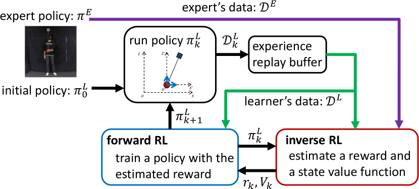
Figure 1: Overall architecture of Entropy-Regularized Imitation Learning (ERIL)

Figure 2: Architecture of two ERIL discriminators: $D_{k}^{(1)}(\bm{x})$ and $D_{k}^{(2)}(\bm{x},\bm{u},\bm{x}^{\prime})$.

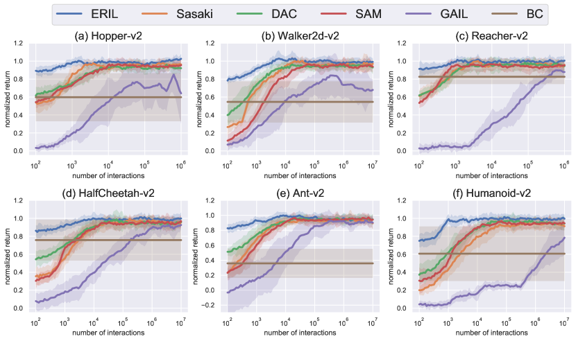
Figure 3: Performance with respect to number of interactions in MuJoCo tasks: Solid lines represent average values, and shaded areas correspond to $\pm 1$ standard deviation region.

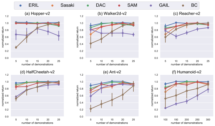
Figure 4: Performance with respect to number of trajectories provided by expert in MuJoCo tasks: Solid lines represent average values, and shaded areas correspond to $\pm 1$ standard deviation region.

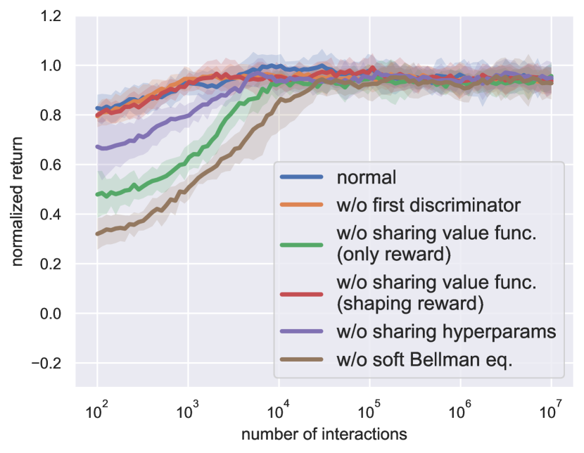
Figure 5: Comparison of learning curves in ablation study

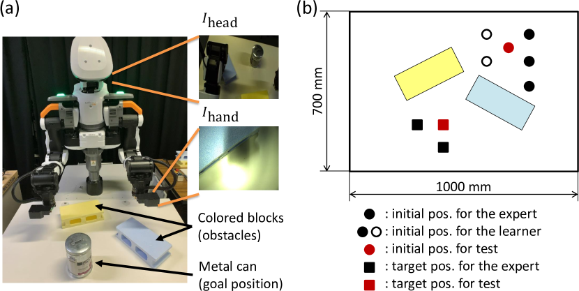
Figure 6: Real robot setting: (a) environment of reaching task, which moves end-effector of left arm to target position; (b) possible environmental configuration.

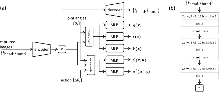
Figure 7: Neural networks used in robot experiment: (a) architecture for policy, reward, state value, state-action value, and first discriminator, sharing the encoder; (b) architecture for encoder: Conv. denotes a convolutional neural network. “$n$c” denotes “$n$ channels.”

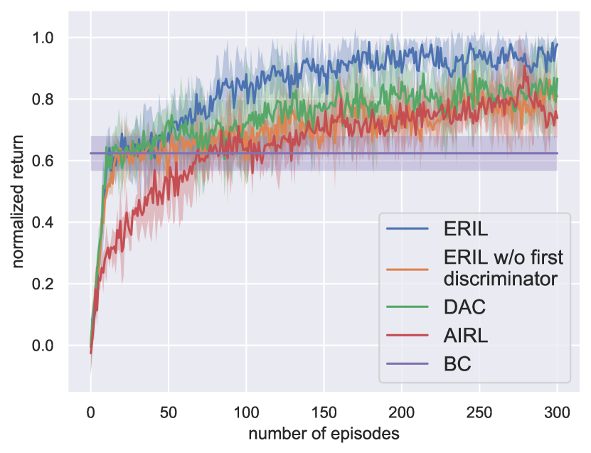
Figure 8: Performance with respect to number of interactions in real robot experiment

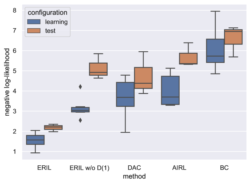
Figure 9: Comparison of NLL in real robot experiment: “ERIL w/o D(1)” denotes ERIL without first discriminator. Note that smaller NLL values indicate a better fit.

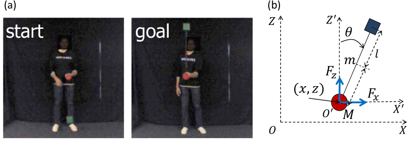
Figure 10: Inverted pendulum task solved by a human subject: (a) start and goal positions; (b) state representation. Notations are explained in C.1.

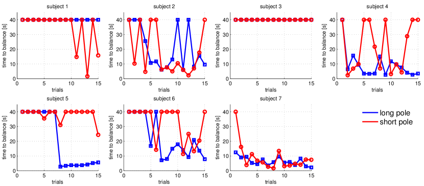
Figure 11: Learning curves of seven subjects: blue: long pole; red: short pole. Trial is considered a failure if subject cannot balance pole in upright position within 40 [s].

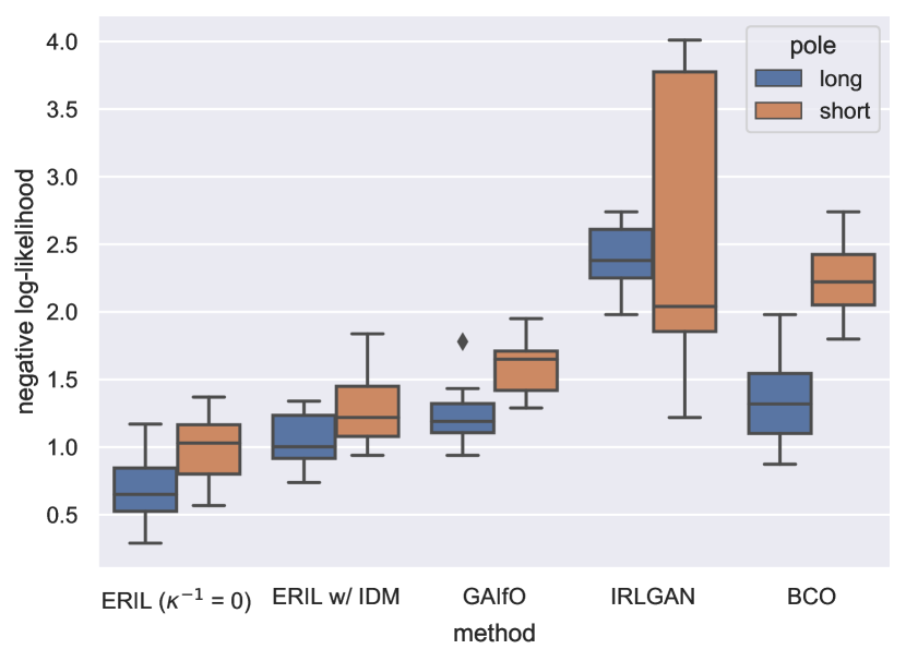
Figure 12: Comparison of NLL among imitation learning algorithms: Note that smaller NLL values indicate a better fit.

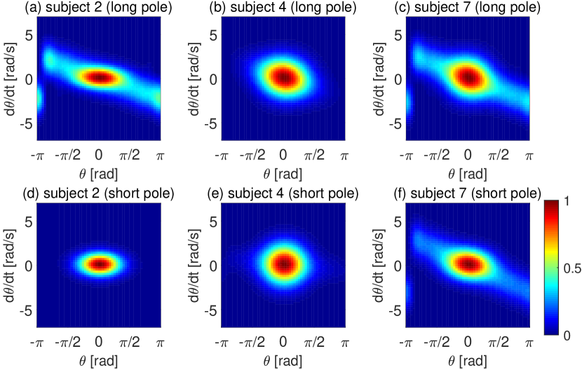
Figure 13: Estimated reward function of Subjects 2, 4, and 7 projected to subspace $(\theta,\omega)$, $\omega=d\theta/dt$

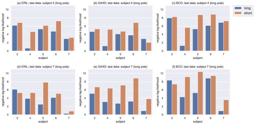
Figure 14: Comparison of NLL when condition of test dataset was different from training one in human inverted pendulum task. Figs. in upper row (a, b, and c) show results when test dataset is $\mathcal{D}_{4,1,\mathrm{te}}^{E}$. Figs. in lower row (d, e, and f) show results when test dataset is $\mathcal{D}_{7,1,\mathrm{te}}^{E}$.

References

- Sutton and Barto (1998) R. Sutton, A. Barto, Reinforcement Learning, MIT Press, 1998.
- Doya (2007) K. Doya, Reinforcement learning: Computational theory and biological mechanisms, HFSP Journal 1 (2007) 30–40.
- Kober et al. (2013) J. Kober, J. A. Bagnell, J. Peters, Reinforcement Learning in Robotics: A Survey, International Journal of Robotics Research 32 (2013) 1238–1274.
- Mnih et al. (2015) V. Mnih, K. Kavukcuoglu, D. Silver, A. A. Rusu, J. Veness, M. G. Bellemare, A. Graves, M. Riedmiller, A. K. Fidjeland, G. Ostrovski, et al., Human-level control through deep reinforcement learning, Nature 518 (2015) 529–533.
- Silver et al. (2017) D. Silver, J. Schrittwieser, K. Simonyan, I. Antonoglou, A. Huang, A. Guez, T. Hubert, et al., Mastering the game of go without human knowledge, Nature 550 (2017) 354–59.
- OpenAI et al. (2019) OpenAI, C. Berner, G. Brockman, B. Chan, V. Cheung, P. Debiak, C. Dennison, et al., Dota 2 with large scale deep reinforcement learning, arXiv preprint (2019).
- Vinyals et al. (2019) O. Vinyals, I. Babuschkin, W. M. Czarnecki, M. Mathieu, A. Dudzik, J. Chung, D. H. Choi, et al., Grandmaster level in StarCraft II using multi-agent reinforcement learning, Nature 575 (2019) 350–54.
- OpenAI et al. (2019) OpenAI, I. Akkaya, M. Andrychowicz, M. Chociej, M. Litwin, B. McGrew, A. Petron, et al., Solving rubik’s cube with a robot hand, arXiv preprint (2019).
- Tsurumine et al. (2019) Y. Tsurumine, Y. Cui, E. Uchibe, T. Matsubara, Deep reinforcement learning with smooth policy update: Application to robotic cloth manipulation, Robotics and Autonomous Systems 112 (2019) 72–83.
- Haarnoja et al. (2018) T. Haarnoja, A. Zhou, K. Hartikainen, G. Tucker, S. Ha, J. Tan, V. Kumar, H. Zhu, A. Gupta, P. Abbeel, S. Levine, Soft actor-critic algorithms and applications, arXiv preprint (2018).
- Wang and Qiao (2019) D. Wang, J. Qiao, Approximate neural optimal control with reinforcement learning for a torsional pendulum device, Neural Networks 117 (2019) 1–7.
- Odekunle et al. (2020) A. Odekunle, M. D. W. Gao, Z.-P. Jiang, Reinforcement learning and non-zero-sum game output regulation for multi-player linear uncertain systems, Automatica 112 (2020).
- Doya and Uchibe (2005) K. Doya, E. Uchibe, The Cyber Rodent project: Exploration of adaptive mechanisms for self-preservation and self-reproduction, Adaptive Behavior 13 (2005) 149–60.
- Ross et al. (2011) S. Ross, G. Gordon, D. Bagnell, A reduction of imitation learning and structured prediction to no-regret online learning, in: Proc. of the 14th International Conference on Artificial Intelligence and Statistics, 2011, pp. 627–35.
- Ng and Russell (2000) A. Y. Ng, S. Russell, Algorithms for inverse reinforcement learning, in: Proc. of the 17th International Conference on Machine Learning, 2000.
- Abbeel and Ng (2004) P. Abbeel, A. Y. Ng, Apprenticeship learning via inverse reinforcement learning, in: Proc. of the 21st International Conference on Machine Learning, 2004.
- Vogel et al. (2012) A. Vogel, D. Ramachandran, R. Gupta, A. Raux, Improving Hybrid Vehicle Fuel Efficiency using Inverse Reinforcement Learning, in: Proc. of the 26th AAAI Conference on Artificial Intelligence, 2012.
- Liu et al. (2013) S. Liu, M. Araujo, E. Brunskill, R. Rossetti, J. Barros, R. Krishnan, Understanding sequential decisions via inverse reinforcement learning, in: Proc. of the 14th IEEE International Conference on Mobile Data Management, IEEE, 2013, pp. 177–186.
- Shimosaka et al. (2014) M. Shimosaka, T. Kaneko, K. Nishi, Modeling risk anticipation and defensive driving on residential roads with inverse reinforcement learning, in: Proc. of the 17th International IEEE Conference on Intelligent Transportation Systems, 2014, pp. 1694–1700.
- Muelling et al. (2014) K. Muelling, A. Boularias, B. Mohler, B. Schölkopf, J. Peters, Learning strategies in table tennis using inverse reinforcement learning., Biological Cybernetics 108 (2014) 603–619.
- Kretzschmar et al. (2016) H. Kretzschmar, M. Spies, C. Sprunk, W. Burgard, Socially compliant mobile robot navigation via inverse reinforcement learning, The International Journal of Robotics Research (2016).
- Xia and El Kamel (2016) C. Xia, A. El Kamel, Neural inverse reinforcement learning in autonomous navigation, Robotics and Autonomous Systems 84 (2016) 1–14.
- Ashida et al. (2019) K. Ashida, T. Kato, K. Hotta, K. Oka, Multiple tracking and machine learning reveal dopamine modulation for area-restricted foraging behaviors via velocity change in caenorhabditis elegans, Neuroscience Letters 706 (2019) 68–74.
- Hirakawa et al. (2018) T. Hirakawa, T. Yamashita, T. Tamaki, H. Fujiyoshi, Y. Umezu, I. Takeuchi, S. Matsumoto, K. Yoda, Can ai predict animal movements? filling gaps in animal trajectories using inverse reinforcement learning, Ecosphere (2018).
- Yamaguchi et al. (2018) S. Yamaguchi, N. Honda, Y. Ikeda, M. Tsukada, S. Nakano, I. Mori, S. Ishii, Identification of animal behavioral strategies by inverse reinforcement learning, PLoS Computational Biology (2018).
- Neu and Szepesvári (2009) G. Neu, C. Szepesvári, Training parsers by inverse reinforcement learning, Machine Learning 77 (2009) 303–337.
- Collette et al. (2017) S. Collette, W. M. Pauli, P. Bossaerts, J. O’Doherty, Neural computations underlying inverse reinforcement learning in the human brain, eLife 6 (2017).
- Fu et al. (2018) J. Fu, K. Luo, S. Levine, Learning robust rewards with adversarial inverse reinforcement learning, in: Proc. of the 6th International Conference on Learning Representations, 2018.
- Ho and Ermon (2016) J. Ho, S. Ermon, Generative adversarial imitation learning, in: Advances in Neural Information Processing Systems 29, 2016, pp. 4565–73.
- Goodfellow et al. (2014) I. Goodfellow, J. Pouget-Abadie, M. Mirza, B. Xu, D. Warde-Farley, S. Ozair, A. Courville, Y. Bengio, Generative adversarial nets, in: Advances in Neural Information Processing Systems 27, 2014, pp. 2672–2680.
- Jena et al. (2020) R. Jena, C. Liu, K. Sycara, Augmenting gail with bc for sample efficient imitation learning, in: Proc. of the 3rd Conference on Robot Learning, 2020.
- Kinose and Taniguchi (2020) A. Kinose, T. Taniguchi, Integration of imitation learning using gail and reinforcement learning using task-achievement rewards via probabilistic graphical model, Advanced Robotics (2020) 1055–1067.
- Sugiyama et al. (2012) M. Sugiyama, T. Suzuki, T. Kanamori, Density ratio estimation in machine learning, Cambridge University Press, 2012.
- Uchibe and Doya (2014) E. Uchibe, K. Doya, Inverse Reinforcement Learning Using Dynamic Policy Programming, in: Proc. of IEEE International Conference on Development and Learning and Epigenetic Robotics, 2014, pp. 222–228.
- Uchibe (2018) E. Uchibe, Model-free deep inverse reinforcement learning by logistic regression, Neural Processing Letters 47 (2018) 891–905.
- Azar et al. (2012) M. G. Azar, V. Gómez, H. J. Kappen, Dynamic policy programming, Journal of Machine Learning Research 13 (2012) 3207–3245.
- Haarnoja et al. (2018) T. Haarnoja, A. Zhou, P. Abbeel, S. Levine, Soft Actor-Critic: Off-policy maximum entropy deep reinforcement learning with a stochastic actor, in: Proc. of the 35th International Conference on Machine Learning, 2018, pp. 1856–1865.
- Kozuno et al. (2019) T. Kozuno, E. Uchibe, K. Doya, Theoretical analysis of efficiency and robustness of softmax and gap-increasing operators in reinforcement learning, in: Proc. of the 22nd International Conference on Artificial Intelligence and Statistics, Okinawa, Japan, 2019, pp. 2995–3003.
- Todorov et al. (2012) E. Todorov, T. Erez, Y. Tassa, MuJoCo: A physics engine for model-based control, in: Proc. of IEEE/RSJ International Conference on Intelligent Robots and Systems, 2012, pp. 5026–5033.
- Brockman et al. (2016) G. Brockman, V. Cheung, L. Pettersson, J. Schneider, J. Schulman, J. Tang, W. Zaremba, OpenAI Gym, arXiv preprint (2016).
- Liu et al. (2021) Z. Liu, X. Li, B. Kang, T. Darrell, Regularization matters in policy optimization – an empirical study on continuous control, in: Proc. of the 9th International Conference on Learning Representations, 2021.
- Parisi et al. (2019) S. Parisi, V. Tangkaratt, J. Peters, M. E. Khan, TD-regularized actor-critic methods, Machine Learning (2019) 1467–1501.
- Ohnishi et al. (2019) S. Ohnishi, E. Uchibe, Y. Yamaguchi, K. Nakanishi, Y. Yasui, S. Ishii, Constrained deep Q-learning gradually approaching ordinary Q-learning, Frontiers in Neurorobotics 13 (2019).
- Li et al. (2018) H. Li, D. Liu, D. Wang, Manifold regularized reinforcement learning, IEEE Transactions on Neural Networks and Learning Systems 29 (2018) 932–43.
- Amit et al. (2020) R. Amit, R. Meir, K. Ciosek, Discount factor as a regularizer in reinforcement learning, in: Proc. of the 37th International Conference on Machine Learning, 2020.
- Ziebart et al. (2008) B. D. Ziebart, A. Maas, J. A. Bagnell, A. K. Dey, Maximum entropy inverse reinforcement learning, in: Proc. of the 23rd AAAI Conference on Artificial Intelligence, 2008.
- Belousov and Peters (2019) B. Belousov, J. Peters, Entropic regularization of Markov decision processes, Entropy 21 (2019) 3207–3245.
- Ahmed et al. (2019) Z. Ahmed, M. N. N. Le Roux, D. Schuurmans, Understanding the impact of entropy on policy optimization, in: Proc. of the 36th International Conference on Machine Learning, 2019, pp. 151–160.
- Pomerleau (1989) D. A. Pomerleau, ALVINN: An autonomous land vehicle in a neural network, in: Advances in Neural Information Processing Systems 1, 1989, pp. 305–313.
- Laskey et al. (2017) M. Laskey, J. Lee, R. Fox, A. Dragan, K. Goldberg, Dart: Noise injection for robust imitation learning, in: Proc. of the 1st Conference on Robot Learning, 2017.
- Torabi et al. (2018) F. Torabi, G. Warnell, P. Stone, Behavioral cloning from observation, in: Proc. of the 27th International Joint Conference on Artificial Intelligence and the 23rd European Conference on Artificial Intelligence, 2018, pp. 4950–57.
- Reddy et al. (2020) S. Reddy, A. D. Dragan, S. Levine, Sqil: Imitation learning via regularized behavioral cloning, in: Proc. of the 8th International Conference on Learning Representations, 2020.
- Kobayashi et al. (2019) K. Kobayashi, T. Horii, R. Iwaki, Y. Nagai, M. Asada, Situated GAIL: Multitask imitation using task-conditioned adversarial inverse reinforcement learning, arXiv preprint (2019).
- Henderson et al. (2018) P. Henderson, W.-D. Chang, P.-L. Bacon, D. Meger, J. Pineau, D. Precup, OptionGAN: Learning joint reward-policy options using generative adversarial inverse reinforcement learning, in: Proc. of the 32nd AAAI Conference on Artificial Intelligence, 2018.
- Torabi et al. (2019) F. Torabi, G. Warnell, P. Stone, Generative adversarial imitation from observation, in: ICML 2019 Workshop on Imitation, Intent, and Interaction, 2019.
- Sun and Ma (2014) M. Sun, X. Ma, Adversarial imitation learning from incomplete demonstrations, in: Proc. of the 28th International Joint Conference on Artificial Intelligence, 2014.
- Blondé and Kalousis (2019) L. Blondé, A. Kalousis, Sample-efficient imitation learning via generative adversarial nets, in: Proc. of the 22nd International Conference on Artificial Intelligence and Statistics, 2019, pp. 3138–3148.
- Lillicrap et al. (2016) T. P. Lillicrap, J. J. Hunt, A. Pritzel, N. Heess, T. Erez, Y. Tassa, D. Silver, D. Wierstra, Continuous control with deep reinforcement learning, in: Proc. of the 4th International Conference on Learning Representations, San Diego, 2016.
- Kostrikov et al. (2019) I. Kostrikov, K. K. Agrawal, D. Dwibedi, S. Levine, J. Tompson, Discriminator-actor-critic: Addressing sample inefficiency and reward bias in adversarial imitation learning, in: Proc. of the 7th International Conference on Learning Representations, 2019.
- Fujimoto et al. (2018) S. Fujimoto, H. van Hoof, D. Meger, Addressing function approximation error in actor-critic methods, in: Proc. of the 35th International Conference on Machine Learning, 2018.
- Sasaki et al. (2019) F. Sasaki, T. Yohira, A. Kawaguchi, Sample efficient imitation learning for continuous control, in: Proc. of the 7th International Conference on Learning Representations, 2019.
- Degris et al. (2012) T. Degris, M. White, R. S. Sutton, Off-policy actor-critic, in: Proc. of the 29th International Conference on Machine Learning, 2012.
- Zuo et al. (2020) G. Zuo, K. Chen, J. Lu, X. Huang, Deterministic generative adversarial imitation learning, Neurocomputing (2020) 60–69.
- Nishio et al. (2020) D. Nishio, D. Kuyoshi, T. Tsuneda, S. Yamane, Discriminator soft actor critic without extrinsic rewards, arXiv preprint (2020).
- Ghasemipour et al. (2019) S. K. S. Ghasemipour, R. Zemel, S. Gu, A divergence minimization perspective on imitation learning methods, in: Proc. of the 3rd Conference on Robot Learning, 2019, pp. 1259–1277.
- Ke et al. (2020) L. Ke, M. Barnes, W. Sun, G. Lee, S. Choudhury, S. Srinivasa, Imitation learning as -divergence minimization, in: Proc. of the 14th International Workshop on the Algorithmic Foundations of Robotics (WAFR), 2020.
- Peters and Schaal (2008) J. Peters, S. Schaal, Reinforcement learning of motor skills with policy gradients, Neural Networks (2008) 1–13.
- Dieng et al. (2019) A. B. Dieng, F. J. R. Ruiz, D. M. Blei, M. K. Titsias, Prescribed generative adversarial networks, arXiv preprint (2019).
- Schaul et al. (2015) T. Schaul, D. Horgan, K. Gregor, D. Silver, Universal value function approximators, in: Proc. of the 32nd International Conference on Machine Learning, 2015, pp. 1312–1320.
- Kingma and Ba (2015) D. Kingma, J. Ba, ADAM: A method for stochastic optimization, in: Proc. of the 3rd International Conference for Learning Representations, 2015.
- Chitta et al. (2012) S. Chitta, I. Sucan, S. Cousins, Moveit! [ROS topics], IEEE Robotics Automation Magazine 19 (2012) 18–19.
- Yarats et al. (2020) D. Yarats, A. Zhang, I. Kostrikov, B. Amos, J. Pineau, R. Fergus, Improving sample efficiency in model-free reinforcement learning from images, arXiv preprint (2020).
- Ghosh et al. (2020) P. Ghosh, M. S. M. Sajjadi, A. Vergari, M. Black, B. Scholkopf, From variational to deterministic autoencoders, in: Proc. of the 7th International Conference on Learning Representations, 2020.
- Wang (2012) J.-J. Wang, Stabilization and tracking control of x-z inverted pendulum with sliding-mode control, ISA Transactions 51 (2012) 763–70.
- Henderson et al. (2018) P. Henderson, R. Islam, P. Bachman, J. Pineau, D. Precup, D. Meger, Deep reinforcement learning that matters, in: Proc. of the 32nd AAAI Conference on Artificial Intelligence, 2018.
- Zhang et al. (2021) B. Zhang, R. Rajan, L. Pineda, N. Lambert, A. Biedenkapp, K. Chua, F. Hutter, R. Calandra, On the importance of hyperparameter optimization for model-based reinforcement learning, in: Proc. of the 24th International Conference on Artificial Intelligence and Statistics, 2021, pp. 4015–23.
- Elfwing et al. (2018) S. Elfwing, E.Uchibe, K. Doya, Online meta-learning by parallel algorithm competition, in: Proc. of the Genetic and Evolutionary Computation Conference, 2018, pp. 426–33.
- Jaderberg et al. (2017) M. Jaderberg, V. Dalibard, S. Osindero, W. M. Czarnecki, J. Donahue, A. Razavi, O. Vinyals, et al., Population based training of neural networks, arXiv preprint (2017).
- Lee et al. (2020) B.-J. Lee, J. Lee, P. Vrancx, D. Kim, K.-E. Kim, Batch reinforcement learning with hyperparameter gradients, in: Proc. of the 37th International Conference on Machine Learning, 2020.