Uncertainty aware Search Framework for Multi-Objective Bayesian Optimization with Constraints

Abstract

We consider the problem of constrained multi-objective (MO) blackbox optimization using expensive function evaluations, where the goal is to approximate the true Pareto set of solutions satisfying a set of constraints while minimizing the number of function evaluations. We propose a novel framework named Uncertainty-aware Search framework for Multi-Objective Optimization with Constraints (USeMOC) to efficiently select the sequence of inputs for evaluation to solve this problem. The selection method of USeMOC consists of solving a cheap constrained MO optimization problem via surrogate models of the true functions to identify the most promising candidates and picking the best candidate based on a measure of uncertainty. We applied this framework to optimize the design of a multi-output switched-capacitor voltage regulator via expensive simulations. Our experimental results show that USeMOC is able to achieve more than 90% reduction in the number of simulations needed to uncover optimized circuits.

1 Introduction

Many engineering and scientific applications involve making design choices to optimize multiple objectives. A representative example includes designing new materials to optimize strength, elasticity, and durability. There are three challenges in solving these kind of optimization problems: 1) The objective functions are unknown and we need to perform expensive experiments to evaluate each candidate design. For example, performing physical lab experiments for material design application. 2) The objectives are conflicting in nature and all of them cannot be optimized simultaneously. 3) The designs that are part of the solution should satisfy a set of constraints. Therefore, we need to find the Pareto optimal set of solutions satisfying the constraints. A solution is called Pareto optimal if it cannot be improved in any of the objectives without compromising some other objective. The overall goal is to approximate the true Pareto set satisfying the constraints while minimizing the number of function evaluations.

Bayesian Optimization (BO) (Shahriari et al. (2016)) is an effective framework to solve blackbox optimization problems with expensive function evaluations. The key idea behind BO is to build a cheap surrogate model (e.g., Gaussian Process (Williams and Rasmussen (2006))) using the real experimental evaluations; and employ it to intelligently select the sequence of function evaluations using an acquisition function, e.g., expected improvement (EI). There is a large body of literature on single-objective BO algorithms (Shahriari et al. (2016); Baptista and Poloczek (2018); Deshwal et al. (2020a, b)) and their applications including hyper-parameter tuning of machine learning methods (Snoek et al. (2012); Kotthoff et al. (2017)). However, there is relatively less work on the more challenging problem of BO for multiple objectives (Knowles (2006); Emmerich and Klinkenberg (2008); Hernández-Lobato et al. (2016); Belakaria et al. (2019, 2020a)) and very limited prior methods to address constrained MO problems (Garrido-Merchán and Hernández-Lobato (2019); Feliot et al. (2017)). PESMOC (Garrido-Merchán and Hernández-Lobato (2019)) is a state-of-the-art approach that relies on the principle of input space entropy search. However, it is computationally expensive to optimize the acquisition function behind PESMOC. A series of approximations are performed to improve the efficiency potentially at the expense of accuracy.

In this paper, we propose a novel Uncertainty-aware Search framework for Multiple Objectives optimizing with Constraints (USeMOC) to overcome the drawbacks of prior methods. The key insight is to improve uncertainty management via a two-stage search procedure to select candidate inputs for evaluation. First, it solves a cheap constrained MO optimization problem defined in terms of the acquisition functions (one for each unknown objective) to identify a list of promising candidates. Second, it selects the best candidate from this list based on a measure of uncertainty. We demonstrate the efficacy of USeMOC over prior methods using a real-world application from the domain of analog circuit design via expensive simulations.

2 Background and Problem Setup

Bayesian Optimization Framework. Let $\mathcal{X}\subseteq\Re^{d}$ be an input space. We assume an unknown real-valued objective function $F:\mathcal{X}\mapsto\Re$, which can evaluate each input $x\in\mathcal{X}$ to produce an evaluation $y$ = $F(x)$. Each evaluation $F(x)$ is expensive in terms of the consumed resources. The main goal is to find an input $x^{*}\in\mathcal{X}$ that approximately optimizes $F$ via a limited number of function evaluations. BO algorithms learn a cheap surrogate model from training data obtained from past function evaluations. They intelligently select the next input for evaluation by trading-off exploration and exploitation to quickly direct the search towards optimal inputs. The three key elements of BO framework are:

1) Statistical Model of $F(x)$. Gaussian Process (GP) (Williams and Rasmussen (2006)) is the most commonly used model. A GP over a space $\mathcal{X}$ is a random process from $\mathcal{X}$ to $\Re$. It is characterized by a mean function $\mu:\mathcal{X}\times\mathcal{X}\mapsto\Re$ and a covariance or kernel function $\kappa$. If a function $F$ is sampled from GP($\mu$, $\kappa$), then $F(x)$ is distributed normally $\mathcal{N}(\mu(x),\kappa(x,x))$ for a finite set of inputs from $x\in\mathcal{X}$.

2) Acquisition Function (Af) to score the utility of evaluating a candidate input $x\in\mathcal{X}$ based on the statistical model. Some popular acquisition functions include expected improvement (EI), upper confidence bound (UCB) and lower confidence bound (LCB). For the sake of completeness, we formally define the acquisition functions employed in this work noting that any other acquisition function can be employed within USeMOC.

$$UCB(x)=\mu(x)+\beta^{1/2}\sigma(x)$$ (1)

$$LCB(x)=\mu(x)-\beta^{1/2}\sigma(x)$$ (2)

$$EI(x)=\sigma(x)(\alpha\Phi(\alpha)+\phi(\alpha)),~{}\alpha=\frac{\tau-\mu(x)}{\sigma(x)}$$ (3)

where $\mu(x)$ and $\sigma(x)$ correspond to the mean and standard deviation of the prediction from statistical model, $\beta$ is a parameter that balances exploration and exploitation; $\tau$ is the best uncovered input; and $\Phi$ and $\phi$ are the CDF and PDF of normal distribution respectively.

3) Optimization Procedure to select the best scoring candidate input according to Af via statistical model, e.g., DIRECT (Jones et al. (1993)).

Multi-Objective Optimization (MOO) Problem with Constraints. Without loss of generality, our goal is to minimize $k\geq 2$ real-valued objective functions $F_{1}(x),F_{2}(x),\cdots,F_{k}(x)$ while satisfying $L$ constraints $C_{1}(x),C_{2}(x),\cdots,C_{L}(x)$ over continuous space $X\subseteq\Re^{d}$. Each evaluation of an input $x\in\mathcal{X}$ produces a vector of objective values $Y$ = $(y_{1},y_{2},\cdots,y_{k})$ where $y_{i}$ = $F_{i}(x)$ for all $i\in\{1,2,\cdots,k\}$ and a vector of constraints values $C$ = $(c_{1},c_{2},\cdots,c_{L})$ where $c_{i}$ = $C_{i}(x)$ for all $i\in\{1,2,\cdots,L\}$. Constraints in real world problems usually take one of the following three forms: [Type 1] $C_{i}$ is a function of the input $x$ and can be expressed declaratively (i.e., white-box constraint); [Type 2] $C_{i}$ is black-box constraint; and [Type 3] $C_{i}$ is a function of both the input $x$ and a combination of the black-box objective functions. We say that a point $x$ Pareto-dominates another point $x^{\prime}$ if $F_{i}(x)\leq F_{i}(x^{\prime})\hskip 2.84526pt\forall{i}$ and there exists some $j\in\{1,2,\cdots,k\}$ such that $F_{j}(x)<F_{j}(x^{\prime})$. The optimal solution of constrained MOO problem is a set of points $\mathcal{X}^{*}\subset\mathcal{X}$ such that no point $x^{\prime}\in\mathcal{X}\setminus\mathcal{X}^{*}$ Pareto-dominates a point $x\in\mathcal{X}^{*}$ and all points in $\mathcal{X}^{*}$ satisfies the problem constraints. The solution set $\mathcal{X}^{*}$ is called the Pareto set and the corresponding set of function values is called the Pareto front. Our goal is to approximate $\mathcal{X}^{*}$ while minimizing the number of function evaluations.

3 Uncertainty-Aware Search Framework

In this section, we provide the details of USeMOC framework for solving constrained multi-objective optimization problems. First, we provide an overview of USeMOC followed by the details of its two main components.

3.1 Overview of USeMOC Framework

USeMOC is an iterative algorithm that involves four key steps. First, We build statistical models $\mathcal{M}_{1},\mathcal{M}_{2},\cdots,\mathcal{M}_{k}$ for each of the $k$ objective functions from the training data in the form of past function evaluations. Second, we select a set of promising candidate inputs $\mathcal{X}_{p}$ by solving a constrained cheap MO optimization problem defined using the statistical models. Specifically, multiple objectives of the cheap MO problem correspond to $\textsc{Af}(\mathcal{M}_{1},x),\textsc{Af}(\mathcal{M}_{2},x),\cdots,\textsc{Af}(\mathcal{M}_{k},x)$ respectively. Any standard acquisition function Af from single-objective BO (e.g., EI, LCB) can be used for this purpose. Additionally, if the constraint is black-box, it is modeled by a GP $\mathcal{M}_{c_{i}}$ and its predictive mean $\mu_{c_{i}}(x)$ is used instead for reasoning. If the value of a constraint $C_{i}$ depends on the evaluation of one (or more) objectives $F_{i}(x)$, we employ the predictive mean $\mu_{i}(x)$. The Pareto set $\mathcal{X}_{p}$ corresponds to the inputs with different trade-offs in the utility space for $k$ unknown functions satisfying the constraints. Third, we select the best candidate input $x_{s}\in\mathcal{X}_{p}$ from the Pareto set that maximizes some form of uncertainty measure for evaluation. Fourth, the selected input $x_{s}$ is used for evaluation to get the corresponding function evaluations: $y_{1}$=$F_{1}(x_{s})$, $y_{2}$=$F_{2}(x_{s})$,$\cdots$,$y_{k}$=$F_{k}(x_{s})$. Algorithm 1 provides the algorithmic pseudocode for USeMOC.

Algorithm 1 USeMOC Framework

Input: $\mathcal{X}$, input space; $F_{1}(x),F_{2}(x),\cdots,F_{k}(x)$, $k$ blackbox objective functions; Af, acquisition function; and $T_{max}$, maximum no. of iterations

1:  Initialize training data of function evaluations $\mathcal{D}$

2:  Initialize statistical models $\mathcal{M}_{1},\cdots,\mathcal{M}_{k},,\mathcal{M}_{C_{0}},\cdots,\mathcal{M}_{C_{m}}$ from $\mathcal{D}$

3:  for each iteration $t$=1 to $T_{max}$ do

4:     // Solve constrained cheap MO problem with objectives Af$(\mathcal{M}_{1},x),\cdots,\textsc{Af}(\mathcal{M}_{k},x)$ to get candidate inputs

5:     $\mathcal{X}_{p}\leftarrow\arg min_{x\in\mathcal{X}}(\textsc{Af}(\mathcal{M}_{1},x),\cdots,\textsc{Af}(\mathcal{M}_{k},x))$     s.t $\mu_{c_{0}},\cdots,\mu_{c_{m}},C_{m+1}\cdots,C_{L}$

6:     // Pick the candidate input with maximum uncertainty

7:     Select $x_{t+1}\leftarrow\arg max_{x\in\mathcal{X}_{p}}\;U_{\beta_{t}}(x)$

8:     Evaluate $x_{t+1}$: $Y_{t+1}\leftarrow(F_{1}(x_{t+1}),\cdots,F_{k}(x_{t+1}))$, $C_{t+1}\leftarrow(C_{0}(x_{t+1}),\cdots,C_{L}(x_{t+1}))$

9:     Aggregate data: $\mathcal{D}\leftarrow\mathcal{D}\cup\{(x_{t+1},Y_{t+1},C_{t+1})\}$

10:     Update models $\mathcal{M}_{1},\cdots,\mathcal{M}_{k},\mathcal{M}_{C_{0}},\cdots,\mathcal{M}_{C_{m}}$ using $\mathcal{D}$

11:     $t\leftarrow t+1$

12:  end for

13:  return Pareto set and Pareto front of $\mathcal{D}$

Advantages. USeMOC has many advantages over prior methods. 1) Provides flexibility to plug-in any acquisition function for single-objective BO. This allows us to leverage existing acquisition functions including EI and LCB. 2) Computationally-efficient to solve constrained MO problems with many objectives. 3) Can handle all three types of constraints (i.e., type 1, type 2, and type 3).

3.2 Key Algorithmic Components of USeMOC

The two main algorithmic components of USeMOC framework are: selecting most promising candidate inputs by solving a cheap constrained MO problem and picking the best candidate via uncertainty maximization. We describe their details below.

Selection of promising candidates. We employ the statistical models $\mathcal{M}_{1},\mathcal{M}_{2},\cdots,\mathcal{M}_{k}$ towards the goal of selecting promising candidate inputs as follows. Given an acquisition function Af (e.g., EI), we construct a constrained cheap multi-objective optimization problem with objectives $\textsc{Af}(\mathcal{M}_{1},x),\textsc{Af}(\mathcal{M}_{2},x),\cdots,\textsc{Af}(\mathcal{M}_{k},x)$, where $\mathcal{M}_{i}$ is the statistical model for unknown function $F_{i}$ and $C_{1},C_{2},\cdots,C_{L}$ are the problem constraints. Generally, there are three types of constraints:

• [Type 1] $C_{i}$ is a function of the input $x$ and can be expressed declaratively (white-box constraint). Such a constraint will take the same form as in the cheap MO problem.

• [Type 2] $C_{i}$ is black-box constraint. In this case, it will be modeled by an independent GP $\mathcal{M}_{c_{i}}$ and predictive mean of its model $\mu_{c_{i}}$ can be used in the optimization process.

• [Type 3] $C_{i}$ is a function of both the input $x$ and a combination of the black-box objective functions. Since verifying constraint $C_{i}$ depends on the evaluation of one (or more) objectives $F_{j}$, we employ the predictive mean(s) $\mu_{i}(x)$ instead.

Without loss of generality and for the sake of notation in Algorithm 1, we suppose that the first $m$ constraints with $0\leq m\leq L$ are black-box.

Since we present the framework as minimization, all AFs will be minimized. The Pareto set $\mathcal{X}_{p}$ obtained by solving this cheap constrained MO problem represents the most promising candidate inputs for evaluation.

$$\mathcal{X}_{p}\leftarrow\arg min_{x\in\mathcal{X}}\; (\textsc{Af}(\mathcal{M}_{1},x),\cdots,\textsc{Af}(\mathcal{M}_{k},x))$$ (4)

$$\textbf{s.t }\mu_{c_{0}},\cdots,\mu_{c_{m}},C_{m+1}\cdots,C_{L}$$

Each acquisition function Af($\mathcal{M}_{i},x$) is dependent on the corresponding surrogate model $\mathcal{M}_{i}$ of the unknown objective function $F_{i}$. Hence, each acquisition function will carry the information of its associated objective function. As iterations progress, using more training data, the models $\mathcal{M}_{1},\mathcal{M}_{2},\cdots,\mathcal{M}_{k}$ will better mimic the true objective functions $F_{1},F_{2},\cdots,F_{k}$. Therefore, the Pareto set of the acquisition function space (solution of Equation 4) becomes closer to the Pareto set of the true functions $\mathcal{X}^{*}$ with increasing iterations.

Intuitively, the acquisition function Af($\mathcal{M}_{i},x$) corresponding to unknown objective function $F_{i}$ tells us the utility of a point $x$ for optimizing $F_{i}$. The input minimizing Af($\mathcal{M}_{i},x$) has the highest utility for $F_{i}$, but may have a lower utility for a different function $F_{j}$ ($j\neq i$). The utility of inputs for evaluation of $F_{j}$ is captured by its own acquisition function Af($\mathcal{M}_{j},x$). Therefore, there is a trade-off in the utility space for all $k$ different functions. The Pareto set $\mathcal{X}_{p}$ obtained by simultaneously optimizing acquisition functions for all $k$ unknown functions will capture this utility trade-off. As a result, each input $x\in\mathcal{X}_{p}$ is a promising candidate for evaluation towards the goal of solving MOO problem. USeMOC employs the same acquisition function for all $k$ objectives. The main reason is to give equivalent evaluation for all functions in the Pareto front (PF) at each iteration. If we use different AFs for different objectives, the sampling procedure would be different. Additionally, the values of various AFs can have considerably different ranges. Thus, this can result in an unbalanced trade-off between functions in the cheap PF leading to the same unbalance in our final PF.

Cheap constrained MO solver. We employ the constrained version of the popular NSGA-II algorithm (Deb et al. (2002a, b)) to solve the MO problem with cheap objective functions and cheap constraints noting that any other algorithm can be used.

Picking the best candidate input. We need to select the best input from the Pareto set $\mathcal{X}_{p}$ obtained by solving the cheap MO problem. All inputs in $\mathcal{X}_{p}$ are promising in the sense that they represent the trade-offs in the utility space corresponding to different unknown functions. It is critical to select the input that will guide the overall search towards the goal of quickly approximating the true Pareto set $\mathcal{X}^{*}$. We employ a uncertainty measure defined in terms of the statistical models $\mathcal{M}_{1},\mathcal{M}_{2},\cdots,\mathcal{M}_{k}$ to select the most promising candidate input for evaluation. In single-objective optimization case, the learned model’s uncertainty for an input can be defined in terms of the variance of the statistical model. For multi-objective optimization case, we define the uncertainty measure as the volume of the uncertainty hyper-rectangle.

$$U_{\beta_{t}}(x)= VOL(\{(LCB(\mathcal{M}_{i},x),UCB(\mathcal{M}_{i},x)\}_{i=1}^{k})$$ (5)

where LCB$(\mathcal{M}_{i},x)$ and UCB$(\mathcal{M}_{i},x)$ represent the lower confidence bound and upper confidence bound of the statistical model $\mathcal{M}_{i}$ for an input $x$ as defined in equations  2 and 3; and $\beta_{t}$ is the parameter value to trade-off exploitation and exploration at iteration $t$. We employ the adaptive rate recommended by (Srinivas et al. (2009)) to set the $\beta_{t}$ value depending on the iteration number $t$. We measure the uncertainty volume measure for all inputs $x\in\mathcal{X}_{p}$ and select the input with maximum uncertainty for function evaluation.

$$x_{t+1}=\arg max_{x\in\mathcal{X}_{p}}\;U_{\beta_{t}}(x)$$ (6)

4 Experiments and Results

In this section, we discuss the experimental evaluation of USeMOC and prior methods on a real-world analog circuit design optimization task. The code for USeMOC is available in github repository: github.com/belakaria/USEMOC.

Analog circuit optimization domain. We consider optimizing the design of a multi-output switched-capacitor voltage regulator via Cadence circuit simulator that imitates the real hardware Belakaria et al. (2020c). Each candidate circuit design is defined by 32 input variables ($d$=32). The first 24 variables are the width, length, and unit of the eight capacitors of the circuit $W_{i},L_{i},M_{i}~{}\forall i\in 1\cdots 8$. The remaining input variables are four output voltage references $V_{ref_{i}}~{}\forall i\in 1\cdots 4$ and four resistances $R_{i}~{}\forall i\in 1\cdots 4$. We optimize nine objectives: maximize efficiency $Eff$, maximize four output voltages $V_{o_{1}}\cdots V_{o_{4}}$, and minimize four output ripples $OR_{1}\cdots OR_{4}$. Our problem has a total of nine constraints:

$${C}_{0}:Cp_{total}\simeq 20nF~{}with~{}Cp_{total}=\sum_{i=1}^{8}(1.955W_{i}L_{i}+0.54(W_{i}+L_{i}))M_{i}$$

$${C}_{1}~{}to~{}{C}_{4}:V_{o_{i}}\geq V_{ref_{i}}~{}\forall\in{1\cdots 4}$$

$${C}_{5}\ to\ {C}_{8\ }:\ \ OR_{lb}\leq OR_{i}\leq OR_{ub}~{}\forall i\ \in{1\cdots 4}$$

$${C}_{9}:Eff\leq 100\%$$

where $OR_{lb}$ and $OR_{ub}$ are the predefined lower-bound and upper-bound of $OR_{i}$ respectively. $Cp_{total}$ is the total capacitance of the circuit. In this problem, $C_{0}$ is a white-box constraint (Type 1), while remaining constraints are combinations of black-box objectives (Type 3).

Multi-objective BO algorithms. We compare USeMOC with the existing BO method PESMOC. Due to lack of BO approaches for constrained MO, we compare to known genetic algorithms (NSGA-II and MOEAD). However, they require large number of function evaluations to converge which is not practical for optimization of expensive functions.

Evaluation Metrics. To measure the performance of baselines and USeMOC, we employ two different metrics, one measuring the accuracy of solutions and another one measuring the efficiency in terms of the number of simulations. 1) Pareto hypervolume (PHV) is a commonly employed metric to measure the quality of a given Pareto front Zitzler (1999). After each iteration $t$ (or number of simulations), we measure the PHV for all algorithms. We evaluate all algorithms for 100 circuit simulations. 2) Percentage gain in simulations is the fraction of simulations our BO algorithm USeMOC is saving to reach the PHV accuracy of solutions at the convergence point of baseline algorithm employed for comparison.

Results and Discussion. We evaluate the performance of USeMOC with two different acquisition functions (EI and LCB) to show the generality and robustness of our approach. We also provide results for the percentage gain in simulations achieved by USeMOC when compared to each baseline method. Figure 1 shows the PHV metric achieved by different multi-objective methods including USeMOC as a function of the number of circuit simulations. We make the following observations: 1) USeMOC with both EI and LCB acquisition functions perform significantly better than all baseline methods. 2) USeMOC is able to uncover a better Pareto solutions than baselines using significantly less number of circuit simulations. This result shows the efficiency of our approach. Table 1 shows that USeMOC achieves percentage gain in simulations w.r.t baseline methods ranging from 90 to 93%.

The analog circuit is implemented in the industry-provided process design kit (PDK) and shows better efficiency and output ripples. Since MOEAD is the best performing baseline optimization method, we use it for the rest of the experimental analysis. Table 2 illustrates the simulated performance of circuit optimized by MOEAD (best baseline) and USeMOC-EI (best variant of our proposed algorithm). Results of both algorithms meet the voltage reference and ripple requirements (100mV) . Compared to MOEAD, the optimized circuit with USeMOC-EI can achieve a higher conversion efficiency of 76.2 % (5.25 % higher than MOEAD, highlighted in red color) with similar output ripples. The optimized circuits can generate the target output voltages within the range of 0.52V-0.61V (1/3x ratio) and 1.07V-1.12V (2/3x ratio) under the loads varying from 14 Ohms to 1697 Ohms (highlighted in black and green colors). Thus, the capability of USeMOC to optimize the parameters of circuit under different output voltage/current conditions is clearly validated. Future work includes improving USeMOC to solve more challenging problems Belakaria et al. (2020b).

Method	MOEAD	NSGA-II	PESMOC
Gain in simulations	90.7%	93.3%	92.5%

Table 1: Percentage gain in simulations achieved by our USeMOC compared to baselines.

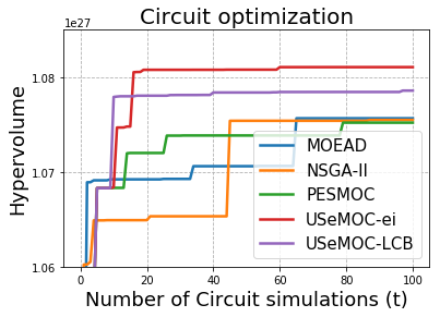
Figure 1: Results of different multi-objective algorithms including USeMOC. The hypervolume metric is shown as a function of the number of circuit design simulations.

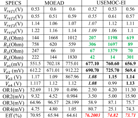
Figure 2: Comparison table of optimized circuit parameters obtained by MOEAD and USeMOC-EI (designs are selected from the Pareto set prioritized by efficiency)

References

- Baptista and Poloczek (2018) Ricardo Baptista and Matthias Poloczek. Bayesian optimization of combinatorial structures. In Proceedings of the 35th International Conference on Machine Learning, pages 462–471, 2018.
- Belakaria et al. (2019) Syrine Belakaria, Aryan Deshwal, and Janardhan Doppa. Max-value entropy search for multi-objective Bayesian optimization. In Proceedings of International Conference on Neural Information Processing Systems (NeurIPS), 2019.
- Belakaria et al. (2020a) Syrine Belakaria, Aryan Deshwal, Nitthilan Kannappan Jayakodi, and Janardhan Rao Doppa. Uncertainty-aware search framework for multi-objective Bayesian optimization. In AAAI Conference on Artificial Intelligence (AAAI), pages 10044–10052, 2020a.
- Belakaria et al. (2020b) Syrine Belakaria, Derek Jackson, Yue Cao, Janardhan Rao Doppa, and Xiaonan Lu. Machine learning enabled fast multi-objective optimization for electrified aviation power system design. In IEEE Energy Conversion Congress and Exposition (ECCE), 2020b.
- Belakaria et al. (2020c) Syrine Belakaria, Zhiyuan Zhou, Aryan Deshwal, Janardhan Rao Doppa, Partha Pande, and Deuk Heo. Design of multi-output switched-capacitor voltage regulator via machine learning. In Proceedings of the Twenty-Third IEEE/ACM Design Automation and Test in Europe Conference (DATE), 2020c.
- Deb et al. (2002a) Kalyanmoy Deb, Amrit Pratap, Sameer Agarwal, T Meyarivan, and A Fast. Nsga-ii. IEEE transactions on evolutionary computation, 6(2):182–197, 2002a.
- Deb et al. (2002b) Kalyanmoy Deb, Amrit Pratap, Sameer Agarwal, and TAMT Meyarivan. A fast and elitist multiobjective genetic algorithm: Nsga-ii. IEEE transactions on evolutionary computation, 6(2):182–197, 2002b.
- Deshwal et al. (2020a) Aryan Deshwal, Syrine Belakaria, and Janardhan Rao Doppa. Scalable combinatorial bayesian optimization with tractable statistical models. CoRR, abs/2008.08177, 2020a. URL https://arxiv.org/abs/2008.08177.
- Deshwal et al. (2020b) Aryan Deshwal, Syrine Belakaria, Janardhan Rao Doppa, and Alan Fern. Optimizing discrete spaces via expensive evaluations: A learning to search framework. In AAAI Conference on Artificial Intelligence (AAAI), pages 3773–3780, 2020b.
- Emmerich and Klinkenberg (2008) Michael Emmerich and Jan-willem Klinkenberg. The computation of the expected improvement in dominated hypervolume of pareto front approximations. Technical Report, Leiden University, 34, 2008.
- Feliot et al. (2017) Paul Feliot, Julien Bect, and Emmanuel Vazquez. A bayesian approach to constrained single-and multi-objective optimization. Journal of Global Optimization, 67(1-2):97–133, 2017.
- Garrido-Merchán and Hernández-Lobato (2019) Eduardo C Garrido-Merchán and Daniel Hernández-Lobato. Predictive entropy search for multi-objective bayesian optimization with constraints. Neurocomputing, 361:50–68, 2019.
- Hernández-Lobato et al. (2016) Daniel Hernández-Lobato, Jose Hernandez-Lobato, Amar Shah, and Ryan Adams. Predictive entropy search for multi-objective bayesian optimization. In International Conference on Machine Learning, pages 1492–1501, 2016.
- Jones et al. (1993) Donald R Jones, Cary D Perttunen, and Bruce E Stuckman. Lipschitzian optimization without the lipschitz constant. Journal of optimization Theory and Applications, 79(1):157–181, 1993.
- Knowles (2006) Joshua Knowles. Parego: a hybrid algorithm with on-line landscape approximation for expensive multiobjective optimization problems. IEEE Transactions on Evolutionary Computation, 10(1):50–66, 2006.
- Kotthoff et al. (2017) Lars Kotthoff, Chris Thornton, Holger H Hoos, Frank Hutter, and Kevin Leyton-Brown. Auto-weka 2.0: Automatic model selection and hyperparameter optimization in weka. The Journal of Machine Learning Research, 18(1):826–830, 2017.
- Shahriari et al. (2016) Bobak Shahriari, Kevin Swersky, Ziyu Wang, Ryan P Adams, and Nando De Freitas. Taking the human out of the loop: A review of bayesian optimization. Proceedings of the IEEE, 104(1):148–175, 2016.
- Snoek et al. (2012) Jasper Snoek, Hugo Larochelle, and Ryan P Adams. Practical bayesian optimization of machine learning algorithms. In Advances in neural information processing systems, pages 2951–2959, 2012.
- Srinivas et al. (2009) Niranjan Srinivas, Andreas Krause, Sham M Kakade, and Matthias Seeger. Gaussian process optimization in the bandit setting: No regret and experimental design. arXiv preprint arXiv:0912.3995, 2009.
- Williams and Rasmussen (2006) Christopher KI Williams and Carl Edward Rasmussen. Gaussian processes for machine learning, volume 2. MIT Press Cambridge, MA, 2006.
- Zitzler (1999) Eckart Zitzler. Evolutionary algorithms for multiobjective optimization: Methods and applications, volume 63. Citeseer, 1999.