Selection on $X_{1}+X_{1}+\cdots X_{m}$ via Cartesian product tree

Abstract

Selection on the Cartesian product is a classic problem in computer science. Recently, an optimal algorithm for selection on $X+Y$, based on soft heaps, was introduced. By combining this approach with layer-ordered heaps (LOHs), an algorithm using a balanced binary tree of $X+Y$ selections was proposed to perform $k$-selection on $X_{1}+X_{2}+\cdots+X_{m}$ in $o(n\cdot m+k\cdot m)$, where $X_{i}$ have length $n$. Here, that $o(n\cdot m+k\cdot m)$ algorithm is combined with a novel, optimal LOH-based algorithm for selection on $X+Y$ (without a soft heap). Performance of algorithms for selection on $X_{1}+X_{2}+\cdots+X_{m}$ are compared empirically, demonstrating the benefit of the algorithm proposed here.

1 Introduction

Sorting all values in $A+B$, where $A$ and $B$ are arrays of length $n$ and $A+B$ is the Cartesian product of these arrays under the $+$ operator, is nontrivial. In fact, there is no known approach faster than naively computing and sorting them which takes $O(n^{2}\log(n^{2}))=O(n^{2}\log(n))$[1]; however, Fredman showed that $O(n^{2})$ comparisons are sufficient[5], though no $O(n^{2})$ algorithm is currently known. In 1993, Frederickson published the first optimal $k$-selection algorithm on $A+B$ with runtime $O(n+k)$[4]. In 2018, Kaplan et al. described another optimal method for $k$-selection on $A+B$, this time in terms of soft heaps[7][3].

In 1978, Johnson and Mizoguchi [6] extended the problem to selecting the $k^{th}$ element in $X_{1}+X_{2}+\cdots+X_{m}$ and did so with runtime $O(m\cdot n^{\lceil\frac{m}{2}\rceil}\log(n))$; however, there has not been significant work done on the problem since. If only the $k^{th}$ value is desired then Johnson and Mizoguchi’s method is the fastest known when $k>m\cdot n^{\lceil\frac{m}{2}\rceil}\log(n)$.

Selection on $X_{1}+X_{2}+\cdots+X_{m}$ is important for max-convolution[2] and max-product Bayesian inference[11, 10]. Computing the $k$ best quotes on a supply chain for a business, when there is a prior on the outcome (such as components from different companies not working together) becomes solving the top values of a probabilistic linear Diophantine equation [9] and thus becomes a selection problem. Finding the most probable isotopologues of a compound such as hemoglobin, $C_{2952}H_{4664}O_{832}N_{812}S_{8}Fe_{4}$, may be done by solving $C+H+O+N+S+Fe$, where $C$ would be the most probable isotope combinations of 2,952 carbon molecules (which can be computed via a multinomial at each leaf, ignored here for simplicity), $H$ would be the most probable isotope combinations of 4,664 hydrogen molecules, and so on. The selection method proposed in this paper has already been used to create the world’s fastest isotopologue calculator[8].

1.1 Layer-ordered heaps

In a standard binary heap, the only known relationships are between a parent and a child: $A_{i}\leq A_{child(i)}$. A layer-ordered heap (LOH) has stricter ordering than the standard binary heap, but is able to be created in $\Omega\left(n\log(\frac{1}{\alpha-1})+\frac{n\cdot\alpha\cdot\log(\alpha)}{\alpha-1}\right)=\Omega(n)$ for constant $\alpha>1$[pennington:optimal]. $\alpha$ is the rank of the LOH and determines how fast the layers grow. A LOH partitions the array into several layers, $L_{i}$, which grow exponentially such that $\frac{|L_{i+1}|}{|L_{i}|}\approx\alpha$ and $|L_{1}|=1$. Every value in a layer $L_{i}$ is $\leq$ every value in proceeding layers $L_{i+1},L_{i+2}\ldots$ which we denote as $L_{i}\leq L_{i+1}$. If $\alpha=1$ then all layers are size one and the LOH is sorted; therefore, to be constructed in $O(n)$ the LOH must have $\alpha>1$.

1.2 Pairwise selection

Serang’s method of selection on $A+B$ utilizes LOHs to be both optimal in theory and fast in practice. The method has four phases. Phase 0 is simply to LOHify (make into a layer-ordered heap) the input arrays.

Phase 1 finds which layer products may be necessary for the $k$-selection. A layer product, $A^{(u)}+B^{(v)}$ is the Cartesian product of layers $A^{(u)}$ and $B^{(v)}$: $A_{1}^{(u)}+B_{1}^{(v)},A_{2}^{(u)}+B_{1}^{(v)},\ldots,A_{1}^{(u)}+B_{2}^{(v)},\ldots$. Finding which layer products are necessary for the selection can be done using a standard binary heap. A layer product is represented in the binary heap in two separate ways: a min tuple $\lfloor(u,v)\rfloor=(min(A^{(u)}+B^{(v)}),(u,v),false)$ and a max tuple $\lceil(u,v)\rceil=(max(A^{(u)}+B^{(v)}),(u,v),true)$. Creating the tuples does not require calculating the Cartesian product of $A^{(u)}+B^{(v)}$ since $min(A^{(u)}+B^{(v)})=min(A^{(u)})+min(B^{(v)})$ which can be found in a linear pass of $A$ and $B$ separately. The same argument applies for $\lceil(u,v)\rceil$. $false$ and $true$ note that the tuple contains the minimum or maximum value in the layer, respectively. Also, let $false=0$ and $true=1$ so that a min tuple is popped before a max tuple even if they contain the same value.

Phase 1 uses a binary heap to retrieve the tuples in sorted order. When a min tuple is popped, the corresponding max tuple and any neighboring layer product’s min tuple is pushed (a set is used to ensure a layer product is only inserted once). When a max tuple is popped, a variable $s$ is increased by $|A^{(u)}+B^{(v)}|=|A^{(u)}|\cdot|B^{(v)}|$ and $(u,v)$ is appended to a list $q$. This continues until $s\geq k$.

In phase 2 and 3 all max tuples still in the heap have their index appended to $q$, then the Cartesian product of all layer products in $q$ are generated. A linear time one-dimensional $k$-select is performed on the values in the Cartesian products to produce only the top $k$ values in $A+B$. The algorithm is linear in the overall number of values produced which is $O(k)$.

In this paper we efficiently perform selection on $X_{1}+X_{2}+\cdots+X_{m}$ by combining the results of pairwise selection problems based on Serang’s method.

2 Methods

In order to retrieve the top $k$ values from $X_{1}+X_{2}+\cdots+X_{m}$, a balanced binary tree of pairwise selections is constructed. The top $k$ values are calculated by selection on $X_{1}+X_{2},X_{3}+X_{4},\ldots$ then on $(X_{1}+X_{2})+(X_{3}+X_{4}),(X_{5}+X_{6})+(X_{7}+X_{8}),\ldots$. All data loaded and generated is stored in arrays which are contiguous in memory, allowing for great cache performance compared to a soft heap based method.

2.1 Tree construction

The tree has height $\lceil\log_{2}(m)\rceil$ with $m$ leaves, each one is a wrapper around one of the input arrays. Upon construction, the input arrays are LOHified in $O(n)$ time, which is amortized into the cost of loading the data. Each node in the tree above the leaves performs pairwise selection on two LOHs, one generated by its left child and one generated by its right child. All nodes in the tree generate their own LOH, but this is done differently for the leaves vs the pairwise selection nodes. When a leaf generates a new layer it simply allows its parent to have access to the values in the next layer of the LOHified input array. For a pairwise selection node, generating a new layer is more involved.

2.2 Pairwise selection nodes

Each node above the leaves is a pairwise selection node. Each pairwise selection node has two children which may be leaves or other pairwise selection nodes. In contrast to the leaves, the pairwise selection nodes will have to calculate all values in their LOHs by generating an entire layer at a time. Generating a new layer requires performing selection on $A+B$, where $A$ is the LOH of its left child and $B$ is the LOH of its right child. Due to the combinatorial nature of this problem, simply asking a child to generate their entire LOH can be exponential in the worst case so they must be generated one layer a time and only as necessary.

The pairwise selection performed is Serang’s method with a few modifications. The size of the selection is always the size of the next layer, $k=|L_{i}|$, to be generated by the parent. The selection begins in the same way as Serang’s: a heap is used to pop min and max layer product tuples. When a min tuple, $\lfloor(u,v)\rfloor$ is popped the values in the Cartesian product are generated and appended to a list of values to be considered in the $k$-selection. The neighboring layer products inserted into the heap are determined using the scheme from Kaplan et al. which differs from Serang’s method. $\lceil(u,v)\rceil,\lfloor(u,2v)\rfloor$, and $\lfloor(u,2v+1)\rfloor$ are always inserted and, if $v=1$, $\lfloor(2u,v)\rfloor,\lfloor(2u+1,v)\rfloor$ are inserted as well. This insertion scheme will not repeat any indices and therefore does not require the use of a set to keep track of the indices in the heap. When any min tuple is proposed, the parent asks both children to generate the layer if it is not already available. If one or both children are not able to generate the layer (i.e. the index is larger the full Cartesian product of the child’s children) then the parent does not insert the tuple into its heap. The newly generated layer is simply appended to the parent’s LOH and may now be accessed by the parent’s parent.

The dynamically generated layers should be kept in individual arrays, then a list of pointers to the arrays may be stored. This avoids resizing a single array every time a new layer is generated.

Theorem 1 in [12] proves that the runtime of the selection is $O(k)$. Lemma 6 and 7 show that the number of items generated in the layer products is $O(n+k)$; however, lemma 7 may be amended to show that any layer product of the form $(u,1)$ or $(1,v)$ will generate $\leq\alpha\cdot|(u-1,1)|\in O(k)$ or $\leq\alpha\cdot|(1,v-1)|\in O(k)$ values, respectively, to show that the total values generated is $O(k)$. Thus the total number of values generated when a parent adds a new layer $L_{i}$ is $O(|L_{i}|)$.

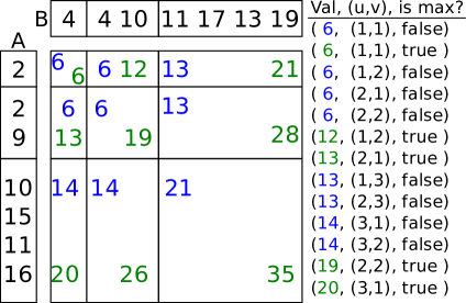
Figure 1: Left: Nine layer products of $A+B$. Right: The order in which the layer product tuples would pop from heap. The two axes are LOHs generated by the left and right children. The values of all 18 possible layer product tuples are shown (nine min tuples in blue and nine max tuples in green). If $k=10$ then the tuples will be popped in the order shown on the right. After $(20,(3,1),true)$ is popped the total number of items in the Cartesian product of all max tuples is $\geq 10$. Note that the values in the layers are not necessarily in sorted order.

2.3 Selection from the root

In order to select the top $k$ values from $X_{1}+X_{2}+\cdots+X_{m}$, the root is continuously asked to generated new layers until the cumulative size the layers in their LOH exceeds $k$. Then a $k$-selection is performed on the layers to retrieve only the top $k$.

The Cartesian product tree is constructed in the same way as the FastSoftTree[kreitzberg:selection] and both dynamically generate new layers in a similar manner with the same theoretical runtime. The pairwise selection methods in both methods create at most $O(\alpha^{2}k)$. Thus the theoretical runtime of both methods is $O(n\cdot m+k\cdot m^{\log_{2}(\alpha^{2})}$ with space usage $O(n\cdot m+k\log(m))$.

2.4 Wobbly version

In Serang’s pairwise selection, after enough layer product tuples are popped from the heap to ensure they contain the top $k$ values, there is normally a selection performed. Strictly speaking, this selection is not necessary anywhere on the tree except for the root when the final $k$ values are returned. When the last max tuple $\lceil(u,v)\rceil$ is popped from the heap, $max(A^{(u)}+B^{(u)})$ is an upper bound on the $k^{th}$ value in the $k$-selection. Instead of doing a $k$-selection and returning the new layer, which requires a linear time selection followed by a linear partition, we can simply do a value partition on $max(A^{(u)}+B^{(u)})$.

A new layer generated from only a value partition and not a selection is not guaranteed to be size $k$, it is at least size $k$ but contains all values $\leq max(A^{(u)}+B^{(u)})$. In the worst case, this may cause layer sizes to grow irregularly with a larger constant than $\alpha$. For example, if $k=2$ and $|L_{1}|=|L_{2}|=1$ then in the worst case every parent will ask their children to each generate two layers and the value partition will not remove any values. Each leaf will generate two values, their parents will then have a new layer of size $2^{2}=4$, their parent will have a new layer of size $(2^{2})^{2}=8$, etc. Thus the root will have to perform a $2$-selection on $2^{m}$ values which will be quite costly.

In an application like calculating the isotopologues of a compound, this version can be quite beneficial. For example, to generate a significant amount of the isotopologues of the titin protein may require $k$ to be hundreds of millions. Titin is made of only carbon, hydrogen, nitrogen, oxygen, and sulfur so it will only have five leaves and a tree height of three. The super-exponential growth of the layers for a tree with height three is now preferential because it will still not create so many more than $k$ values but it will do so in many fewer layers with only value partitions and not the more costly linear selections. We call this the “wobbly” Cartesian product tree.

3 Results

All experiments were run on a workstation equipped with 256GB of RAM and two AMD Epyc 7351 processors running Ubuntu 18.04.4 LTS.

k	Cartesian product tree	FastSoftTree
$2^{2}$	$1.404\times 10^{-03}$	$3.146\times 10^{-03}$
$2^{3}$	$1.504\times 10^{-03}$	$2.855\times 10^{-03}$
$2^{4}$	$1.521\times 10^{-03}$	$3.163\times 10^{-03}$
$2^{5}$	$1.592\times 10^{-03}$	$2.618\times 10^{-03}$
$2^{6}$	$1.689\times 10^{-03}$	$4.172\times 10^{-03}$
$2^{7}$	$1.718\times 10^{-03}$	$4.830\times 10^{-03}$
$2^{8}$	$1.881\times 10^{-03}$	$8.864\times 10^{-03}$
$2^{9}$	$2.080\times 10^{-03}$	$0.01143$
$2^{10}$	$1.745\times 10^{-03}$	$0.01792$
$2^{11}$	$2.217\times 10^{-03}$	$0.02362$
$2^{12}$	$3.123\times 10^{-03}$	$0.04459$
$2^{13}$	$3.318\times 10^{-03}$	$0.07026$
$2^{14}$	$5.099\times 10^{-03}$	$0.111$
$2^{15}$	$6.240\times 10^{-03}$	$0.2296$
$2^{16}$	$8.724\times 10^{-03}$	$0.4952$
$2^{17}$	$0.01266$	$0.9609$
$2^{18}$	$0.01663$	$1.610$
$2^{19}$	$0.02684$	$12.77$
$2^{20}$	$0.0405$	$25.53$

Table 1: Runtimes for Cartesian product tree vs FastSoftTree with $n=32$, $m=256$ and $\alpha=1.1$. The runtime is averaged over 20 iterations. For small problems the soft heap based tree is competitive with the Cartesian product tree; however, for large enough $k$ the cache performance of the LOH significantly outperforms the soft heap resulting in a $630.4\times$ speedup for $k=2^{20}$.

In a Cartesian product tree, replacing the pairwise X+Y selection steps from Kaplan et al.’s soft heap-based algorithm with Serang’s optimal LOH-based method provides the same $o(n\cdot m+k\cdot m)$ theoretical performance for the Cartesian product tree, but is practically much faster (Table 1. This is particularly true when $k\cdot m^{\log 2(\alpha^{2})}\gg n\cdot m$, where popping values dominates the cost of loading the data. When $k\geq 2^{10}$, $k\cdot m^{0.2750}<n\cdot m$ which is reflected in our results where for $k=2^{20}$ we get a $630.4\times$ speedup, significantly larger than for $k=2^{10}$ which only has a $10.27\times$ speedup.

k	Standard version	Wobbly version
$2^{2}$	$1.544\times 10^{-04}$	$1.777\times 10^{-04}$
$2^{3}$	$1.754\times 10^{-04}$	$1.468\times 10^{-04}$
$2^{4}$	$2.086\times 10^{-04}$	$1.846\times 10^{-04}$
$2^{5}$	$2.386\times 10^{-04}$	$2.046\times 10^{-04}$
$2^{6}$	$2.080\times 10^{-04}$	$1.935\times 10^{-04}$
$2^{7}$	$3.060\times 10^{-04}$	$2.672\times 10^{-04}$
$2^{8}$	$3.481\times 10^{-04}$	$3.225\times 10^{-04}$
$2^{9}$	$4.289\times 10^{-04}$	$2.978\times 10^{-04}$
$2^{10}$	$6.119\times 10^{-04}$	$4.087\times 10^{-04}$
$2^{11}$	$7.976\times 10^{-04}$	$4.585\times 10^{-04}$
$2^{12}$	$1.000\times 10^{-03}$	$7.263\times 10^{-04}$
$2^{13}$	$1.711\times 10^{-03}$	$1.189\times 10^{-03}$
$2^{14}$	$2.344\times 10^{-03}$	$1.465\times 10^{-03}$
$2^{16}$	$7.531\times 10^{-03}$	$4.890\times 10^{-03}$
$2^{15}$	$3.919\times 10^{-03}$	$2.578\times 10^{-03}$
$2^{17}$	$0.0113$	$9.090\times 10^{-03}$
$2^{18}$	$0.01741$	$0.01583$
$2^{19}$	$0.02777$	$0.02511$
$2^{20}$	$0.04904$	$0.04228$
$2^{21}$	$0.08572$	$0.07773$
$2^{22}$	$0.1623$	$0.1424$
$2^{23}$	$0.3274$	$0.234$
$2^{24}$	$0.636$	$0.4838$
$2^{25}$	$1.210$	$1.029$
$2^{26}$	$2.306$	$1.588$
$2^{27}$	$4.993$	$3.487$
$2^{28}$	$9.995$	$8.441$
$2^{29}$	$19.7$	$14.31$
$2^{30}$	$43.45$	$24.33$

Table 2: Runtimes for standard Cartesian product tree vs wobbly Cartesian product tree with $n=256$, $m=5$ and $\alpha=1.1$. The runtime averaged over 20 iterations for the two methods. With $m=5$ the tree only has three layers and so the super-exponential growth of the layers as they go from the leaves to the roots does not become intractable. As $k$ becomes extremely large the ability of the wobbly tree to generate huge layers at the root without performing any selections significantly reduces the runtime resulting in a $1.786\times$ speedup.

As we see in Table 2, for small $m$ the Cartesian product tree can gain significant increases in performance when there are no linear selections performed in the tree and the layers are allowed to grow super-exponentially. As $k$ grows, the speedup of the wobbly version continues to grow, resulting in a $1.786\times$ speedup for $k=2^{30}$. When $m\gg 5$ the growth of the layers near the root start to significantly hurt the performance. For example, if $n=32,m=256$ and $k=256$ the wobbly version takes $0.5805$ seconds and produces 149,272 values at the root compared to the non-wobbly version which takes $1.8810\times 10^{-03}$ seconds and produces just 272 values at the root.

4 Discussion

Replacing pairwise selection which uses a soft heap with Serang’s optimal method provides a significant increase in performance. Since both methods LOHify the input arrays (using the same LOHify method) the most significant increases are seen when $k\cdot m^{\log 2(\alpha^{2})}\gg n\cdot m$. For small $m$, the performance can boosted using the wobbly version; however for large $m$ the super-exponentially sized layers can quickly begin to dampen performance. It may be possible to limit the layer sizes in the wobbly version by performing selections only at certain layers of the tree: either by performing the selection on every $i^{th}$ layer or only on the top several layers.

Any method reminiscent of the Kaplan et al. proposal scheme, which uses a scheme whereby each value retrieved from the soft heap inserts a constant number, $c\geq 1$, of new values into the soft heap, requires implicit construction of a LOH.

Optimal, online computation of values requires retrieving the top $k_{1}$ values and then top $k_{2}$ remaining values and so on. The number of corrupt values is bounded by $\epsilon\cdot I$, where $I$ insertions have been performed to date; therefore, there are at most $\epsilon\cdot c\cdot k_{1}$ corrupt values. The top $k_{1}$ values can be retrieved by popping no more than $k_{1}+\epsilon\cdot c\cdot k_{1}$ values from the soft heap and then performing $k_{1}$-selection (via median-of-medians) on the resulting popped values. The $\epsilon\cdot k_{1}$ corrupt values are reinserted into the soft heap, bringing the total insertions to $k_{1}\cdot\epsilon\cdot(1+c)$. To retrieve the top $k_{2}$ remaining values, $k_{2}+\epsilon\cdot k_{1}\cdot\epsilon\cdot(1+c)\in\Omega(k_{2}+k_{1})$ values need to be popped. These top $k_{2}$ values can be retrieved in optimal $O(k_{2})$ time if $k_{2}\in\Theta(k_{1})$. Likewise, $k_{3}\in\Theta(k_{1}+k_{2})$, and so on. Thus, the sequence of $k$ values must grow exponentially.

Rebuilding the soft heap (rather than reinserting the corrupted values into the soft heap) instead does not alleviate this need for exponential growth in $k_{1},k_{2},\ldots$ required to achieve optimal $O(k_{1}+k_{2}+\cdots)$ total runtime. When rebuilding, each next $k_{j}$ must be comparable to the size of the entire soft heap (so that the cost of rebuilding can be amortized out by the optimal $\Theta(k_{j})$ steps used to retrieve the next $k_{j}$ values). Because $c\geq 1$, the size of the soft heap is always $\geq k_{1}+k_{2}+\cdots+k_{j-1}$ for the selections already performed, and thus the rebuilding cost is $k_{1}+k_{2}+\cdots+k_{j-1}$, which must be $\in\Theta(k_{j})$. This likewise requires exponential growth in the $k_{j}$.

This can be seen as the layer ordering property, which guarantees that a proposal scheme such as that in Kaplan et al. does not penetrate to great depth in the combinatorial heap, which could lead to exponential complexity when $c>1$. In this manner, the $k_{1},k_{2},\ldots$ values can be seen to form layers of heap, which would not require retrieving further layers before the current extreme layer has been exhausted.

This method has already proved to be beneficial in generating the top $k$ isotopologues of chemical compounds, but it is not limited to this use-case. It is applicable to fast algorithms for inference on random variables $Y=X_{1}+X_{2}+\cdots+X_{m}$ in the context of graphical Bayesian models. It may not generate a value at every index in a max-convolution, but it may generate enough values fast enough to give a significant result.

References

- [1] D. Bremner, T. M. Chan., E. D. Demaine, J. Erickson, F. Hurtado, J. Iacono, S. Langerman, and P. Taslakian. Necklaces, convolutions, and . In Algorithms–ESA 2006, pages 160–171. Springer, 2006.
- [2] M. Bussieck, H. Hassler, G. J. Woeginger, and U. T. Zimmermann. Fast algorithms for the maximum convolution problem. Operations research letters, 15(3):133–141, 1994.
- [3] B. Chazelle. The soft heap: an approximate priority queue with optimal error rate. Journal of the ACM (JACM), 47(6):1012–1027, 2000.
- [4] G. N. Frederickson. An optimal algorithm for selection in a min-heap. Information and Computation, 104(2):197–214, 1993.
- [5] M. L. Fredman. How good is the information theory bound in sorting? Theoretical Computer Science, 1(4):355–361, 1976.
- [6] D. Johnson and T. Mizoguchi. Selecting the element in and . SIAM Journal on Computing, 7(2):147–153, 1978.
- [7] H. Kaplan, L. Kozma, O. Zamir, and U. Zwick. Selection from heaps, row-sorted matrices and using soft heaps. Symposium on Simplicity in Algorithms, pages 5:1–5:21, 2019.
- [8] P. Kreitzberg, J. Pennington, K. Lucke, and O. Serang. Fast exact computation of the most abundant isotope peaks with layer-ordered heaps. Analytical Chemistry, 92(15):10613–10619, 2020.
- [9] P. Kreitzberg and O. Serang. Toward a unified approach for solving probabilistic linear diophantine equations. 2020.
- [10] J. Pfeuffer and O. Serang. A bounded -norm approximation of max-convolution for sub-quadratic Bayesian inference on additive factors. Journal of Machine Learning Research, 17(36):1–39, 2016.
- [11] O. Serang. A fast numerical method for max-convolution and the application to efficient max-product inference in Bayesian networks. Journal of Computational Biology, 22:770–783, 2015.
- [12] O Serang. Optimal selection on X + Y simplified with layer-ordered heaps. arXiv preprint arXiv:2001.11607, 2020.