The first open channel for a yield-stress fluid in complex porous media

Abstract

The prediction of the first fluidized path of a yield-stress fluid in complex porous media is a challenging yet an important task to understand the fundamentals of fluid flow in several industrial and biological processes. In most cases, the conditions that open this first path are known either through experiments or expensive computations. Here, we present a simple network model to predict the first open channel for a yield-stress fluid in a complex porous medium. For porous media made of non-overlapping disks, we find that the pressure drop required to open the first channel for given yield stress depends on both the relative disks size to the macroscopic length of the system and the packing fraction. We also report the statistics on the arc-length of the first open path. Finally, we discuss the implication of our results on the design of porous media used in energy storage applications.

I Introduction

Fluid flow in porous media is studied for more than a century due to its high relevance to several engineering applications such as enhanced oil recovery Green et al. (1998); Farajzadeh et al. (2012); Fraggedakis et al. (2015); Sahimi (2011), filtration and separation Herzig et al. (1970); Tien and Payatakes (1979); Jaisi et al. (2008), fermentation Pandey (2003); Aufrecht et al. (2019), soil sequestration Schlesinger (1999), energy storage Duduta et al. (2011); Sun et al. (2019), and food processing Greenkorn (1983). In most cases, the fluids involved in these applications exhibit yield stress/viscoplastic behavior Bonn and Denn (2009); Balmforth et al. (2014). Therefore, understanding the conditions – critical pressure drop and/or stresses – that lead to fluidization of yield-stress fluids in porous media can help boost the efficiency and lower the operational cost of several industrial applications.

In pressure-driven flows, the critical pressure drop $\Delta P_{c}$ required to fluidize the yield-stress fluid and open the first channel Chen et al. (2005); Hewitt et al. (2016); Waisbord et al. (2019) depends on the heterogeneous geometric characteristics and porosity $1-\phi$ of the porous medium, where $\phi$ is the volume fraction of the solid phase Talon et al. (2013); Bauer et al. (2019); Chaparian and Tammisola (2020). Therefore, it is crucial to understand the relation between the yielding conditions and the structure of the porous medium, which will lead to predictive models for both the first open channel and $\Delta P_{c}$.

The classical way to study yield-stress fluids is by solving the Cauchy momentum equations using viscoplastic constitutive relations, such as the Bingham and Herschel–Bulkley models Bird et al. (1987); Huilgol and Phan-Thien (2015); Saramito (2016a). More recently, though, there is an increasing trend on using elastoviscoplastic Saramito (2007) and kinematic hardening Dimitriou and McKinley (2019) models that originate from continuum mechanics Gurtin et al. (2010); Anand and Govindjee (2020). The yield stress behavior, however, leads to an ill-defined problem that does not describe the stress distribution within the unyielded regions of the fluid Balmforth et al. (2014); Saramito and Wachs (2017). Common ways to resolve this problem is by using either optimization- Hestenes (1969); Powell (1978); Glowinski (2008) or regularization-based methods Papanastasiou (1987); Frigaard and Nouar (2005). The former are accurate on predicting the yielded/unyielded boundaries and the flow field Dimakopoulos et al. (2013), however, they are computationally expensive Saramito (2016b) for conditions nearby the yield limit. Although the latter reduce the computational cost, they introduce non-physical parameters Tsamopoulos et al. (2008); Dimakopoulos et al. (2018) that lead to non-physical solutions, incorrect location of yield/unyield boundaries, and inaccurate yield limits Mitsoulis and Tsamopoulos (2017); Frigaard and Nouar (2005). Here, we are interested in determining the statistics of the critical $\Delta P_{c}$ for a yield-stress fluid in complex porous media. Thus, we need to use models that can predict accurately and efficiently $\Delta P_{c}$ along with the first open channel.

Fluid flow in porous media is traditionally described through network models Fatt et al. (1956) that represent the complex geometric characteristics of the domain with spherical pore throats and cylindrical edges Alim et al. (2017); Bryant et al. (1993); Blunt (2001); Blunt et al. (2013); Stoop et al. (2019). In addition to their wide applicability in Newtonian fluids, network models have also been applied to describe $\Delta P_{c}$ and the flow behavior with respect to the applied pressure drop in yield-stress fluids Chen et al. (2005); Frigaard et al. (2017); Liu et al. (2019); Talon and Hansen (2020). When the relation between the local flow rate and the pressure drop is known, the network representation allows for the use of graph theoretic tools Kharabaf and Yortsos (1997); Chen et al. (2005); Balhoff et al. (2012); Liu et al. (2019) to quickly evaluate $\Delta P_{c}$ and the flow response of the system. In general, though, the results of network viscoplastic models in complex porous media have been rarely compared and validated against those produced by solving the full fluid problem, and thus the conditions of their validity/applicability are unknown.

The goal of the present work is to predict the first open channel for a yield-stress fluid in a complex porous medium along with the critical applied pressure drop required to open it. We develop a simple network model based on realistic porous media configurations, and use graph theoretical tools to study the statistics of yielding conditions in terms of the medium porosity. We validate our results against reported pressure-driven simulations of Bingham fluids in porous media. Finally, we discuss the relevance of our study to applications such as enhanced oil recovery and propose possible extensions.

II Theory

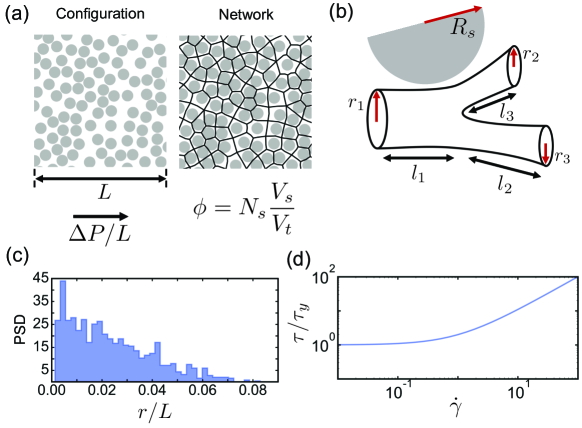
Figure 1: (a) Typical configuration of a porous medium of length $L$ and porosity $1-\phi$ that is made of non-overlapping monodisperse spheres of radius $R_{s}$, and its network representation. Across the domain, a macroscopic pressure gradient $\Delta P/L$ is applied to fluidize the yield-stress fluid. (b) Schematic of three network edges with different radii $r_{i}$ and lengths $l_{i}$ ($i=1,2,3$ ). The network representation includes the local geometric characteristics of the complex porous medium structure. (c) Characteristic pore-size distribution for the network shown in (a) as derived from the network model. (d) Typical shear stress response $\tau$ as a function of the applied shear rate $\dot{\gamma}$ of a viscoplastic fluid with yield stress $\tau_{y}$.

II.1 Network topology

We are interested in the construction of realistic network models that capture the complex morphology of real porous media. The main scope of our work is to understand the statistics on the critical conditions that lead to fluidization in terms of the porosity $1-\phi$ and topological characteristics of the medium.

To first approximation, we assume a porous medium that consists of monodisperse non-overlapping spheres/disks of radius $R_{s}$ as shown in Fig. 1(a). It is apparent that the structure of void space depends on the solid volume fraction defined as $\phi=N_{s}V_{s}/V_{t}$, where $N_{s}$ is the total number of spheres, $V_{s}$ is the volume of an individual sphere and $V_{t}$ the total volume of the system. We can use the given porous medium structure and create the network representation shown in the right panel of Fig. 1(a).

The network consists of nodes and edges that span the entire medium, where its complex topological characteristics are encoded on the connectivity between them Gostick (2017); Khan et al. (2019). Additionally, the local geometric characteristics of the porous medium are included on the length $l_{i}$ and radius $r_{i}$ of each individual edge, Fig. 1(b). For demonstration, we show in Fig. 1(c) the pore size distribution for the configuration of Fig. 1(a). Details on the generation of porous media with monodisperse non-overlaping sphere, the construction of the network representation, and the choice of $r_{i}$ and $l_{i}$ are given in the Appendix of the paper.

II.2 Yield-stress fluid in a network

Yield-stress fluids are characterized by their solid-liquid transition when the Euclidean norm of the stress field exceeds the value of yield stress (Von Mises criterion) Gurtin et al. (2010); Hill (1998). The typical shear stress response in simple shear flow is shown in Fig. 1(d), where for $\dot{\gamma}\rightarrow 0$ the shear stress reaches its critical value $\tau\rightarrow\tau_{y}$. The most common constitutive relations used to describe yield-stress fluids are the Bingham and the Herschel-Bulkley models Bird et al. (1987). Both of them, though, have the same behavior for $\dot{\gamma}\rightarrow 0$. Therefore, it is sufficient to discuss only the Bingham model for a porous medium to understand the connection between the yielding conditions to the geometric and topological characteristics of the network.

For pressure-driven flows, the local flow rate $q_{i}$ of edge $i$ is described in terms of the local geometric properties $r_{i},l_{i}$, the local pressure drop along the edge $\Delta P_{i}$, and the yield stress $\tau_{y}$ of the fluid as Bird et al. (1987); Liu et al. (2019); Frigaard (2019)

$$q_{i}=\left\{\begin{array}[]{cc}\frac{r_{i}^{4}}{l_{i}}\left(\Delta P_{i}-\frac{\tau_{y}l_{i}}{r_{i}}\right)&\text{for}\,\,\Delta P_{i}>\frac{\tau_{y}l_{i}}{r_{i}}\\ 0&\text{ for}\,\,\left\lvert\Delta P_{i}\right\rvert<\frac{\tau_{y}l_{i}}{r_{i}}\\ \frac{r_{i}^{4}}{l_{i}}\left(\Delta P_{i}+\frac{\tau_{y}l_{i}}{r_{i}}\right)&\text{ for}\,\,\Delta P_{i}<-\frac{\tau_{y}l_{i}}{r_{i}}\\ \end{array}\right.$$ (1)

Near the no-flow limit $q_{i}\rightarrow 0$, we see from Eq. 1 that $\Delta P_{i}\rightarrow\tau_{y}l_{i}/r_{i}$, and thus smaller in radius or longer in length channels require larger applied pressure drop to yield. Across the first open channel, we can calculate the total pressure drop across the medium to be $\Delta P\equiv\sum_{i=1}^{N}\Delta P_{i}=\tau_{y}\sum_{i=1}^{N}l_{i}/r_{i}$, where $N$ is the total number of edges across the path. From this expression, we can see that the connectivity between the edges determines the first open channel in a real porous medium, and it corresponds to the path of ‘least resistance’. Thus, the problem of finding $\Delta P_{c}$ can be formulated as finding the path of the minimum pressure drop as follows Liu et al. (2019)

$$\frac{\Delta P_{c}}{\tau_{y}}=\min_{C\in\mathcal{C}_{\text{in-out}}}\sum_{i=1}^{N}\frac{l_{i}}{r_{i}}$$ (2)

where $\mathcal{C}_{\text{in-out}}$ is the set of all paths between the corresponding boundaries.

The problem of Eq. 2 satisfies the principle of minimum dissipation rate and is valid near equilibrium Kondepudi and Prigogine (2014). In particular, the entropy production for a pressure-driven flow is $\sigma_{D}=q\Delta P$ De Groot and Mazur (2013). Thus, for conditions near the solid-liquid transition where $q\rightarrow 0^{+}$, the minimum pressure drop path also minimizes $\sigma_{D}$.

To solve Eq. 2, we transform the generated network into a graph with edges that have weights equal to $l_{i}/r_{i}$ and use the Dijkstra method Dijkstra et al. (1959) for directed graphs to determine the first open channel. This method is known to scale quadratically with the path length West et al. (1996); Bollobás (2013), and therefore for complex domains that lead to larger number of edges the computational cost increases. For a single porous medium configuration, however, the overall computational time to determine the first open channel is much lower (seconds to minutes) than that required to solve the full fluid flow problem using optimization methods (days to weeks) Dimakopoulos et al. (2018); Chaparian and Tammisola (2020).

III Results

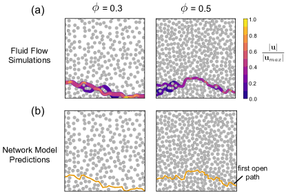
Figure 2: Validation of the network model for the first open channel against simulations for a pressure-driven Bingham fluid in a complex porous medium with $R_{s}/L=0.02$. (a) Simulation results of the open pathway for conditions near the critical pressure drop $\Delta P_{c}$. The contour plot shows the magnitude of the local velocity, normalized with the maximum velocity across the channel. (b) Network model predictions for the first open channel. The cases of $\phi=0.3$ and $\phi=0.5$ are examined. It is clear that both the full Bingham fluid simulation and the network model predict the same location for the first open channel.

III.1 The first open channel

When the applied pressure drop approaches the critical value $\Delta P\rightarrow\Delta P_{c}^{+}$, there exists a single open channel across the entire medium. Here, we test the validity of the proposed approach to determine the first open channel nearby when the solid-liquid transition occurs. For comparison, we solve the full flow field under pressure-driven conditions for a yield-stress fluid for the complex porous media shown in Fig. 2. We consider the cases of $\phi=0.3$ and $\phi=0.5$, respectively. All the lengths are normalized with the macroscopic length of the system $L$ and also $R_{s}/L=0.02$. For simplicity, we use two-dimensional porous media, however, our approach is general and does not depend on the dimensionality of the problem.

Figure 2(a) shows the normalized velocity magnitude that results from the solution of the Cauchy momentum equation for a Bingham fluid Chaparian and Tammisola (2020). Also, Fig. 2(b) depicts the predictions for the first open channel after solving the minimization problem of Eq. 2. In both cases, the network model is able to reproduce the results of the fluid problem for the first open path.

Notably, in both cases of Fig. 2(a), where the full fluid flow problem is solved, we can see the existence of additional paths other than the one predicted by the network model. We justify this observation based on the fact that the fluid flow simulations are performed at extremely large, yet finite non-dimensional yield stress (i.e. Bingham number; see Chaparian and Tammisola (2020)). Indeed, we speculate that for simulations with $q\rightarrow 0^{+}$ (i.e. infinite Bingham number), the secondary paths will eventually close and only the predicted one by the network model will be present. However, as it is clear from the Fig. 2(a), flow rate in those secondary paths are negligible and does not contribute to the leading order of the resistance.

III.2 Critical pressure drop $\Delta P_{c}$ and its statistics in complex porous media

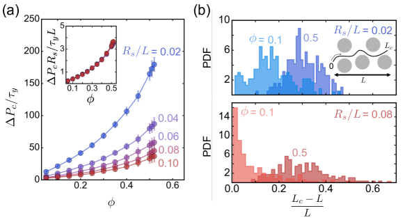
Figure 3: Statistics on the predictions of the network model for 500 realizations per value of $\phi$. (a) Critical pressure drop $\Delta P_{c}$ as a function of the volume fraction $\phi$ for different ratio of $R_{s}/L$. $\Delta P_{c}$ is normalized with the yield stress of the fluid $\tau_{y}$. The error bars indicate the variance around the mean value. Inset – Scaled critical pressure drop $\Delta P_{c}R_{s}/\tau_{y}L$ in terms of $\phi$. For non-overlapping spheres, the results for different $R_{s}/L$ collapse in a master curve. (b) Probability density distributions for the normalized arc-length of the first open channel $L_{c}/L-1$. The cases of $R_{s}/L=0.02$ and $R_{s}/L=0.08$ are shown, respectively, for $\phi=0.1$ and $\phi=0.5$. In general, increasing $\phi$ leads to increase of $\Delta P_{c}$ required to open the first channel, but also leads to a wide distribution of arc-lengths, which provide large uncertainty on the critical macroscopic pressure gradient $\Delta P_{c}/L_{c}$ required to yield the fluid in the porous medium.

In addition to the first open path, the network model can predict the normalized critical pressure $\Delta P_{c}$ required to yield the fluid in the porous medium.

$\phi$	$\frac{\Delta P_{c}}{\tau_{y}}$ Network	$\frac{\Delta P_{c}}{\tau_{y}}$ Simulations	Rel. Error $\%$
$0.1$	$22.16$	$22.63$	$1.87$
$0.3$	$61$	$65.2$	$6.43$
$0.5$	$142.16$	$145.28$	$2.05$

Table 1: Predicted normalized critical pressure drop $\Delta P_{c}$ required to open the first open channel for the configurations shown in Fig. 2. We show both the predictions of the network model and the full simulation results, along with the relative error $\frac{\Delta P_{c}^{\text{sim}}-\Delta P_{c}^{\text{net}}}{\Delta P_{c}^{\text{sim}}}$. The network model is adequate on predicting both the first open channel and the critical pressure drop required to open it.

In table 1 we show the predictions of the normalized critical pressure drop $\Delta P_{c}/\tau_{y}$ for both the network model and the full simulations. For $\phi=0.3$ and $0.5$ we consider the configurations shown in Fig. 2. In all cases, it is clear that the relative difference of $\Delta P_{c}$ between the two models never exceeds $6.5\%$. The negligible difference can be justified by the fact that discussed above about the secondary paths, or/and the simplification of the geometric characteristics of the medium by its network representation. We conclude, though, that network-based models are adequate to predict both the first open path and the critical pressure drop required to open it.

The validation of the model allows us to predict $\Delta P_{c}$ as a function of $\phi$ and the geometric characteristics of the system. For a porous medium made of non-overlapping disks, we control the microstructure characteristics by changing the ratio $R_{s}/L$. For each combination of $\phi$ and $R_{s}/L$, we generate 500 realizations for gathering the statistics of $\Delta P_{c}$.

Figure 3(a) shows the normalized critical pressure drop $\Delta P_{c}/\tau_{y}$ in terms of $\phi$. The colored lines indicate different value of $R_{s}/L\in[0.02,0.1]$, while the error bars correspond to the variance of the statistical sample. For all $R_{s}/L$ the normalized pressure drop increases with increasing $\phi$. This behavior is expected as the radius $r_{i}$ of each edge decreases monotonically as $\phi$ increases Torquato and Haslach Jr (2002). Additionally, we observe that decreasing the ratio $R_{s}/L$ leads to increase in $\Delta P_{c}$, in qualitative agreement with experiments Waisbord et al. (2019). The reason for this behavior can be explained by examining the arc-length (defined as $L_{c}=\sum_{i}^{N}l_{i}$) for the first open channel.

Figure 3(b) illustrates the histogram of $L_{c}$ for $\phi=0.3$ and $0.5$ as well as $R_{s}/L=0.02$ and $0.08$. In both cases we observe that increasing solid volume fraction leads to an increase in the total length of the first open path. While large $\phi$ results in almost similar behavior for both $R_{s}/L$, it is apparent that decreasing the size of the spheres results in more tortuous paths, even for low solid volume fraction.

Dimensional analysis on Eq. 2 indicates that $\Delta P_{c}$ follows a simple scaling with $R_{s}/L$. In particular, by rescaling the local edge radius $r_{i}$ with the sphere radius $R_{s}$, we find $\Delta\widetilde{P}_{c}=\Delta P_{c}R_{s}/\tau_{y}L=\sum_{i=1}^{N}\left(l_{i}/L\right)\left(R_{s}/r_{i}\right)$. The inset in Fig. 3(a) shows the rescaled form of the critical pressure drop for all $R_{s}/L$, were for non-overlapping disks, a master curve exists for all the examined values of $\phi$. The dependence of $\Delta\widetilde{P}_{c}$ with $\phi$, the effect of the pore microstructure, as well as the physical mechanism for the behavior of the tortuosity $\tau=L_{c}/L$ will be presented in a future work.

IV Discussion

We find that network models provide an efficient and accurate way to model the fluidization conditions in porous media. They are also accurate in locating the first open channel, which is equivalent to the path of least resistance through the entire medium.

Our results on the normalized critical pressure drop $\Delta P_{c}/\tau_{y}$ can be used to design porous media systems with the desired flow properties. In applications such as semi-solid flow batteries Duduta et al. (2011), it is critical to keep the contact between the active material (electrode particles) and the conductive wiring (carbon nanoparticle network) intact during operation, otherwise there is a significant energy loss during cycling of the battery Solomon et al. (2018); Wei et al. (2015). This can be achieved by immersing the active material and the electronically conductive agent in yield-stress fluids like Carbopol Zhu et al. (2020). Therefore, we can use the predicted $\Delta P_{c}/\tau_{y}$ to determine the size of the active particles to optimize the design and operation of semi-solid electrodes.

The present model can also provide insights on the design of porous media. By taking advantage of the computational efficiency of the proposed network model, we can perform on-the-fly optimization to construct porous media with optimal mixing and transport properties Lester et al. (2013); Kirkegaard and Sneppen (2020). Such ideas have recently been implemented in elastic networks with optimal phonon band structures Ronellenfitsch et al. (2019a, b), and we believe they can also be used for designing porous media immersed in yield-stress fluids.

Given their inherent node/edge structure, network models are fairly simple to be analyzed using graph theoretical tools. The unique property of yield-stress fluid, namely the fluidization conditions, allows us to use algorithms that can find the minimum resistance pathways with minimal efforts. In coarse-grained domains, however, where the microscopic geometric irregularities are encoded in the heterogeneous ‘permeability’ tensor Hewitt et al. (2016), graph theory tools might not be the most suitable ones. An alternative way to calculate the first open channel in a continuum with spatially variable properties is through methodologies used in physical chemistry to identify reaction pathways Henkelman et al. (2000); Swenson et al. (2018). There, the first open channel corresponds to the path that passes through the minimum energy barrier, namely the transition state point.

The present model considers only the case of viscoplastic materials and disregards the fluid elasticity Saramito (2007); Cheddadi et al. (2012); Fraggedakis et al. (2016a, b) prior to yielding. Therefore, further analysis is required to connect the yield criterion to the elastic modulus of the fluid, which can provide insights for engineering both the porous medium and the fluid itself. Additionally, the yielding and/or stoppage conditions might be further affected by possible thixotropic Mewis and Wagner (2012) and kinematic hardening Dimitriou and McKinley (2019); Gurtin et al. (2010) phenomena.

V Summary

In this work, we presented a network model for yield-stress fluids in porous media that describe the effects of porosity $1-\phi$ and microstructure properties in complex geometries. We demonstrated the capabilities of the model to predict the critical applied pressure drop required to open the first channel in the medium. Also, we compared our results to direct numerical simulations of the full fluid problem for Bingham fluids and we showed the accuracy and computational efficiency of the network-based models to solid-liquid transition. Finally, we discussed the implications of our model on the optimization and design of porous media.

Contributions

D.F. conceptualized, designed, and performed the analysis in the present study. E.C. and O.T. provided the fluid flow simulation results. D.F. wrote the manuscript. All authors contributed to the final manuscript.

Appendix

Porous medium and network generation

For the generation of porous media that consist of non-overlapping disks, we implemented the random sequential addition (RSA) algorithm Zhang and Torquato (2013); Cule and Torquato (1999); Torquato et al. (2006). The procedure described in Torquato et al. (2006) allows for the fast generation of randomly packed disks with the desired volume fractions. Due to the constraint of non-overlapping disks, all generated microstructures never exceed $\phi=0.52$ in two dimensions.

For the generation of the network model, we implemented the maximal ball algorithm as described in Silin and Patzek (2006); Dong and Blunt (2009); Al-Kharusi and Blunt (2007). The procedure allows us to get the radius $r_{i}$ and length $l_{i}$ for each edge. The maximal ball algorithm represents ‘fits’ a circle/sphere within each pore Alim et al. (2017), its radius of which represents the $r_{i}$ we use in Eq. 2. Other choices of $r_{i}$ can be considered (e.g. equivalent radius etc.), however, our choice for the local radius works well in predicting both the first open channel and the critical pressure drop required to open it. The generated network was represented by a graph with vertices $V$ and edges $E$ using the open source library NetworkX Hagberg et al. (2008).

Details on the numerical simulation of the fluid flow problem shown in Fig. 2(a) can be found in Chaparian and Tammisola (2020).

References

- Green et al. (1998) D. W. Green, G. P. Willhite, et al., Enhanced oil recovery, Vol. 6 (Henry L. Doherty Memorial Fund of AIME, Society of Petroleum Engineers …, 1998).
- Farajzadeh et al. (2012) R. Farajzadeh, A. Andrianov, R. Krastev, G. Hirasaki, and W. R. Rossen, Advances in colloid and interface science 183, 1 (2012).
- Fraggedakis et al. (2015) D. Fraggedakis, C. Kouris, Y. Dimakopoulos, and J. Tsamopoulos, Physics of Fluids 27, 082102 (2015).
- Sahimi (2011) M. Sahimi, Flow and transport in porous media and fractured rock: from classical methods to modern approaches (John Wiley & Sons, 2011).
- Herzig et al. (1970) J. Herzig, D. Leclerc, and P. L. Goff, Industrial & Engineering Chemistry 62, 8 (1970).
- Tien and Payatakes (1979) C. Tien and A. C. Payatakes, AIChE journal 25, 737 (1979).
- Jaisi et al. (2008) D. P. Jaisi, N. B. Saleh, R. E. Blake, and M. Elimelech, Environmental science & technology 42, 8317 (2008).
- Pandey (2003) A. Pandey, Biochemical Engineering Journal 13, 81 (2003).
- Aufrecht et al. (2019) J. A. Aufrecht, J. D. Fowlkes, A. N. Bible, J. Morrell-Falvey, M. J. Doktycz, and S. T. Retterer, PloS one 14, e0218316 (2019).
- Schlesinger (1999) W. H. Schlesinger, “Carbon sequestration in soils,” (1999).
- Duduta et al. (2011) M. Duduta, B. Ho, V. C. Wood, P. Limthongkul, V. E. Brunini, W. C. Carter, and Y.-M. Chiang, Advanced Energy Materials 1, 511 (2011).
- Sun et al. (2019) H. Sun, J. Zhu, D. Baumann, L. Peng, Y. Xu, I. Shakir, Y. Huang, and X. Duan, Nature Reviews Materials 4, 45 (2019).
- Greenkorn (1983) R. A. Greenkorn, Flow phenomena in porous media: fundamentals and applications in petroleum, water and food production (Marcel Dekker, New York, NY, USA, 1983).
- Bonn and Denn (2009) D. Bonn and M. M. Denn, Science 324, 1401 (2009).
- Balmforth et al. (2014) N. J. Balmforth, I. A. Frigaard, and G. Ovarlez, Annual Review of Fluid Mechanics 46, 121 (2014).
- Chen et al. (2005) M. Chen, W. Rossen, and Y. C. Yortsos, Chemical engineering science 60, 4183 (2005).
- Hewitt et al. (2016) D. Hewitt, M. Daneshi, N. Balmforth, and D. Martinez, Journal of Fluid Mechanics 790, 173 (2016).
- Waisbord et al. (2019) N. Waisbord, N. Stoop, D. M. Walkama, J. Dunkel, and J. S. Guasto, Physical Review Fluids 4, 063303 (2019).
- Talon et al. (2013) L. Talon, H. Auradou, M. Pessel, and A. Hansen, EPL (Europhysics Letters) 103, 30003 (2013).
- Bauer et al. (2019) D. Bauer, L. Talon, Y. Peysson, H. Ly, G. Batôt, T. Chevalier, and M. Fleury, Physical Review Fluids 4, 063301 (2019).
- Chaparian and Tammisola (2020) E. Chaparian and O. Tammisola, arXiv preprint arXiv:2004.02950 (2020).
- Bird et al. (1987) R. B. Bird, R. C. Armstrong, and O. Hassager, (1987).
- Huilgol and Phan-Thien (2015) R. R. Huilgol and N. Phan-Thien, Fluid mechanics of viscoplasticity (Springer, 2015).
- Saramito (2016a) P. Saramito, Complex fluids (Springer, 2016).
- Saramito (2007) P. Saramito, Journal of Non-Newtonian Fluid Mechanics 145, 1 (2007).
- Dimitriou and McKinley (2019) C. J. Dimitriou and G. H. McKinley, Journal of Non-Newtonian Fluid Mechanics 265, 116 (2019).
- Gurtin et al. (2010) M. E. Gurtin, E. Fried, and L. Anand, The mechanics and thermodynamics of continua (Cambridge University Press, 2010).
- Anand and Govindjee (2020) L. Anand and S. Govindjee, Continuum Mechanics of Solids (Oxford University Press, USA, 2020).
- Saramito and Wachs (2017) P. Saramito and A. Wachs, Rheologica Acta 56, 211 (2017).
- Hestenes (1969) M. R. Hestenes, Journal of optimization theory and applications 4, 303 (1969).
- Powell (1978) M. J. Powell, Mathematical programming 14, 224 (1978).
- Glowinski (2008) R. Glowinski, Lectures on numerical methods for non-linear variational problems (Springer Science & Business Media, 2008).
- Papanastasiou (1987) T. C. Papanastasiou, Journal of Rheology 31, 385 (1987).
- Frigaard and Nouar (2005) I. Frigaard and C. Nouar, Journal of non-newtonian fluid mechanics 127, 1 (2005).
- Dimakopoulos et al. (2013) Y. Dimakopoulos, M. Pavlidis, and J. Tsamopoulos, Journal of Non-Newtonian Fluid Mechanics 200, 34 (2013).
- Saramito (2016b) P. Saramito, Journal of Non-Newtonian fluid mechanics 238, 6 (2016b).
- Tsamopoulos et al. (2008) J. Tsamopoulos, Y. Dimakopoulos, N. Chatzidai, G. Karapetsas, and M. Pavlidis, Journal of Fluid Mechanics 601, 123 (2008).
- Dimakopoulos et al. (2018) Y. Dimakopoulos, G. Makrigiorgos, G. Georgiou, and J. Tsamopoulos, Journal of Non-Newtonian Fluid Mechanics 256, 23 (2018).
- Mitsoulis and Tsamopoulos (2017) E. Mitsoulis and J. Tsamopoulos, Rheologica Acta 56, 231 (2017).
- Fatt et al. (1956) I. Fatt et al., Transactions of the AIME 207, 144 (1956).
- Alim et al. (2017) K. Alim, S. Parsa, D. A. Weitz, and M. P. Brenner, Physical review letters 119, 144501 (2017).
- Bryant et al. (1993) S. L. Bryant, P. R. King, and D. W. Mellor, Transport in porous media 11, 53 (1993).
- Blunt (2001) M. J. Blunt, Current opinion in colloid & interface science 6, 197 (2001).
- Blunt et al. (2013) M. J. Blunt, B. Bijeljic, H. Dong, O. Gharbi, S. Iglauer, P. Mostaghimi, A. Paluszny, and C. Pentland, Advances in Water resources 51, 197 (2013).
- Stoop et al. (2019) N. Stoop, N. Waisbord, V. Kantsler, V. Heinonen, J. S. Guasto, and J. Dunkel, Journal of Non-Newtonian Fluid Mechanics 268, 66 (2019).
- Frigaard et al. (2017) I. A. Frigaard, K. G. Paso, and P. R. de Souza Mendes, Rheologica Acta 56, 259 (2017).
- Liu et al. (2019) C. Liu, A. De Luca, A. Rosso, and L. Talon, Physical review letters 122, 245502 (2019).
- Talon and Hansen (2020) L. Talon and A. Hansen, Physics of Porous Media (2020).
- Kharabaf and Yortsos (1997) H. Kharabaf and Y. C. Yortsos, Physical Review E 55, 7177 (1997).
- Balhoff et al. (2012) M. Balhoff, D. Sanchez-Rivera, A. Kwok, Y. Mehmani, and M. Prodanović, Transport in porous media 93, 363 (2012).
- Gostick (2017) J. T. Gostick, Physical Review E 96, 023307 (2017).
- Khan et al. (2019) Z. A. Khan, T. Tranter, M. Agnaou, A. Elkamel, and J. Gostick, Computers & Chemical Engineering 123, 64 (2019).
- Hill (1998) R. Hill, The mathematical theory of plasticity, Vol. 11 (Oxford university press, 1998).
- Frigaard (2019) I. Frigaard, in Lectures on Visco-Plastic Fluid Mechanics (Springer, 2019) pp. 1–40.
- Kondepudi and Prigogine (2014) D. Kondepudi and I. Prigogine, Modern thermodynamics: from heat engines to dissipative structures (John Wiley & Sons, 2014).
- De Groot and Mazur (2013) S. R. De Groot and P. Mazur, Non-equilibrium thermodynamics (Courier Corporation, 2013).
- Dijkstra et al. (1959) E. W. Dijkstra et al., Numerische mathematik 1, 269 (1959).
- West et al. (1996) D. B. West et al., Introduction to graph theory, Vol. 2 (Prentice hall Upper Saddle River, NJ, 1996).
- Bollobás (2013) B. Bollobás, Modern graph theory, Vol. 184 (Springer Science & Business Media, 2013).
- Torquato and Haslach Jr (2002) S. Torquato and H. Haslach Jr, Appl. Mech. Rev. 55, B62 (2002).
- Solomon et al. (2018) B. R. Solomon, X. Chen, L. Rapoport, A. Helal, G. H. McKinley, Y.-M. Chiang, and K. K. Varanasi, ACS Applied Energy Materials 1, 3614 (2018).
- Wei et al. (2015) T.-S. Wei, F. Y. Fan, A. Helal, K. C. Smith, G. H. McKinley, Y.-M. Chiang, and J. A. Lewis, Advanced Energy Materials 5, 1500535 (2015).
- Zhu et al. (2020) Y. Zhu, T. M. Narayanan, M. Tułodziecki, H. Sanchez-Casalongue, Q. Horn, L. Meda, Y. Yu, J. Sun, T. Regier, G. H. McKinley, et al., Sustainable Energy & Fuels (2020).
- Lester et al. (2013) D. R. Lester, G. Metcalfe, and M. Trefry, Physical review letters 111, 174101 (2013).
- Kirkegaard and Sneppen (2020) J. B. Kirkegaard and K. Sneppen, Physical Review Letters 124, 208101 (2020).
- Ronellenfitsch et al. (2019a) H. Ronellenfitsch, N. Stoop, J. Yu, A. Forrow, and J. Dunkel, Physical Review Materials 3, 095201 (2019a).
- Ronellenfitsch et al. (2019b) H. Ronellenfitsch, J. Dunkel, et al., Frontiers in Physics 7, 178 (2019b).
- Henkelman et al. (2000) G. Henkelman, B. P. Uberuaga, and H. Jónsson, The Journal of chemical physics 113, 9901 (2000).
- Swenson et al. (2018) D. W. Swenson, J.-H. Prinz, F. Noe, J. D. Chodera, and P. G. Bolhuis, Journal of chemical theory and computation 15, 813 (2018).
- Cheddadi et al. (2012) I. Cheddadi, P. Saramito, and F. Graner, Journal of rheology 56, 213 (2012).
- Fraggedakis et al. (2016a) D. Fraggedakis, Y. Dimakopoulos, and J. Tsamopoulos, Journal of Non-Newtonian Fluid Mechanics 236, 104 (2016a).
- Fraggedakis et al. (2016b) D. Fraggedakis, Y. Dimakopoulos, and J. Tsamopoulos, Soft matter 12, 5378 (2016b).
- Mewis and Wagner (2012) J. Mewis and N. J. Wagner, Colloidal suspension rheology (Cambridge University Press, 2012).
- Zhang and Torquato (2013) G. Zhang and S. Torquato, Physical Review E 88, 053312 (2013).
- Cule and Torquato (1999) D. Cule and S. Torquato, Journal of applied physics 86, 3428 (1999).
- Torquato et al. (2006) S. Torquato, O. Uche, and F. Stillinger, Physical Review E 74, 061308 (2006).
- Silin and Patzek (2006) D. Silin and T. Patzek, Physica A: Statistical mechanics and its applications 371, 336 (2006).
- Dong and Blunt (2009) H. Dong and M. J. Blunt, Physical review E 80, 036307 (2009).
- Al-Kharusi and Blunt (2007) A. S. Al-Kharusi and M. J. Blunt, Journal of petroleum science and engineering 56, 219 (2007).
- Hagberg et al. (2008) A. Hagberg, P. Swart, and D. S Chult, Exploring network structure, dynamics, and function using NetworkX, Tech. Rep. (Los Alamos National Lab.(LANL), Los Alamos, NM (United States), 2008).