A Non-Abelian Generalization of the Alexander Polynomial from Quantum $\mathfrak{sl}_{3}$

Abstract.

Murakami and Ohtsuki have shown that the Alexander polynomial is an $R$-matrix invariant associated with representations $V(t)$ of unrolled restricted quantum $\mathfrak{sl}_{2}$ at a fourth root of unity. In this context, the highest weight $t\in\mathbb{C}^{\times}$ of the representation determines the polynomial variable. For any semisimple Lie algebra $\mathfrak{g}$ of rank $n$, we extend their construction to a link invariant $\Delta_{\mathfrak{g}}$, which takes values in $n$-variable Laurent polynomials. The focus of this paper is the case $\mathfrak{g}=\mathfrak{sl}_{3}$. For any knot $K$, evaluating $\Delta_{\mathfrak{sl}_{3}}$ at ${t_{1}=1}$, ${t_{2}=1}$, or ${t_{2}=it_{1}^{-1}}$ recovers the Alexander polynomial of $K$. This is not obvious from an examination of the $R$-matrix, as the $R$-matrix evaluated at these parameters does not satisfy the Alexander-Conway skein relation. We tabulate $\Delta_{\mathfrak{sl}_{3}}$ for all knots up to seven crossings along with various other examples. In particular, it distinguishes the Kinoshita-Terasaka knot and Conway knot mutant pair and is nontrivial on the Whitehead double of the trefoil.

1. Introduction

Since the introduction of the Jones polynomial, an outstanding problem in quantum topology has been to give interpretations of quantum invariants of knots and 3-manifolds in terms of invariants from classical topology. Our motivating example is the Alexander-Conway polynomial, realized as the quantum invariant from unrolled restricted quantum $\mathfrak{sl_{2}}$ at a primitive fourth root of unity. In [Mur92, Mur93, Oht02], Murakami and Ohtuski construct the Alexander-Conway polynomial from Turaev-type [Tur88] $R$-matrix actions on a family of quantum group representations. We denote these representations by $V(t)$, with $t\in\mathbb{C}^{\times}$ the highest weight of this two dimensional Verma module.

In contrast to the Jones polynomial, whose variable is the quantum parameter $q$ of $U_{q}(\mathfrak{sl_{2}})$, the variable in the Alexander-Conway polynomial is the parameter $t\in\mathbb{C}^{\times}$ of the unrolled restricted quantum group representation $V(t)$. Unlike the standard representation of $U_{q}(\mathfrak{sl_{2}})$, $V(t)$ has quantum dimension zero; therefore, the naive $R$-matrix invariant assigns the value of zero to any closed tangle. Instead, using a modified trace [GPT09], given by computing the invariant after cutting an arbitrary strand of the link, yields a nontrivial invariant.

Although many higher rank quantum invariants have been defined in the literature, they are not as well understood as quantum invariants in rank one. The HOMFLY, Kauffman, and Kuperberg polynomials [Kau90, FHL⁺85, Kup94] are higher rank versions of the Jones polynomial. The Links-Gould invariants, among others, generalize the Alexander polynomial as an $R$-matrix invariant from quantum supergroups [LG92, KS91, GP07]. However, a higher rank version of the Alexander polynomial from unrolled restricted quantum groups has not been studied and is the subject of this paper. Specifically, we generalize the ADO invariants to higher rank at $q^{2}=-1$ [ADO92].

Let $\Delta^{+}$ denote the positive roots of a Lie algebra $\mathfrak{g}$ of rank $n$. Each character $t$, which we identify with $(t_{1},\dots,t_{n})\in(\mathbb{C}^{\times})^{n}\cong\text{Map}(\Delta^{+},\mathbb{C}^{\times})$, determines a Verma module $V({\smash{\text{\boldmath{$t$}}}})$ over the restricted quantum group $\overline{U}_{\zeta}(\mathfrak{g})$, which is studied further in [Har19b]. We assume $q=\zeta$ is a primitive fourth root of unity and extend $V({\smash{\text{\boldmath{$t$}}}})$ to a representation of the unrolled restricted quantum group. The associated quantum invariant $\Delta_{\mathfrak{g}}$ is an assignment of a Laurent polynomial in $\mathbb{Z}[t_{1}^{\pm},\dots,t_{n}^{\pm}]$ to every link $L$, and it is computed from a modified trace by coloring each component of $L$ by $V({\smash{\text{\boldmath{$t$}}}})$.

This invariant is not to be confused with the multivariable Alexander polynomial. In particular, the number of variables in $\Delta_{\mathfrak{g}}$ depends on the rank of $\mathfrak{g}$ and not on the number of components of $L$. In fact, we compare $\Delta_{\mathfrak{sl}_{3}}$ with the Alexander polynomial and other invariants in the Statement of Results. However, if $L$ has $m$ components, one can consider a modified version of $\Delta_{\mathfrak{g}}$ by coloring each component of $L$ by a distinct representation $V({\smash{\text{\boldmath{$t$}}}})$. We discuss this multi-colored invariant briefly, but our focus here is the singly-colored invariant.

1.1. Statement of Results

The value of $\Delta_{\mathfrak{sl}_{3}}$ on all prime knots up to seven crossings is tabulated in Figure 10. We have also computed this invariant for some higher crossing knots, allowing us to compare it with the Alexander, Jones, and HOMFLY polynomials. These values are found in Figure 11.

Most notable in these examples is that the Conway knot $\mathsf{11_{n34}}$ and the Kinoshita-Terasaka knot $\mathsf{11_{n42}}$ have different $\Delta_{\mathfrak{sl}_{3}}$ polynomials. Therefore, this invariant can detect mutation. Our observation is consistent with the following result of Morton and Cromwell [MC96]: Colorings by representations with a multiplicity-free tensor product cannot detect mutation. The polynomial invariants of $\mathsf{11_{n34}}$ and $\mathsf{11_{n42}}$ are determined from Figure 1 below, as explained in Section 7.

In addition to $\mathsf{11_{n34}}$ and $\mathsf{11_{n42}}$, untwisted Whitehead doubles of knots have Alexander polynomial equal to 1 [Rol03]. It follows that the Alexander module of each of these knots is zero. We take the Whitehead double of the trefoil $\text{Wh}^{0}(\mathsf{3_{1}})$ as an example. In contrast to the Alexander invariant, $\Delta_{\mathfrak{sl}_{3}}$ assigns a non-trivial polynomial to these knots, see Figures 1 and 2.

The Alexander-Conway polynomial $\Delta$ is dominated by $\Delta_{\mathfrak{sl}_{3}}$ on knots and it is in the following sense that $\Delta_{\mathfrak{sl}_{3}}$ can be interpreted as a two-variable generalization of the classical knot invariant.

[Reduction to the Alexander-Conway Polynomial]thmplugin Let $K$ be a knot. Then

$$\Delta_{\mathfrak{sl}_{3}}(K)(t,\pm 1)=\Delta_{\mathfrak{sl}_{3}}(K)(\pm 1,t)=\Delta_{\mathfrak{sl}_{3}}(K)(t,\pm it^{-1})=\Delta(K)(t^{4}).$$ (1)

Moreover, these are the only substitutions that yield the Alexander polynomial on all knots.

(a) $\mathsf{11_{n34}}$

(b) $\mathsf{11_{n42}}$

Figure 1. The value of $\Delta_{\mathfrak{sl}_{3}}$ on the mutant pair $\mathsf{11_{n34}}$ and $\mathsf{11_{n42}}$.

(a) $\text{Wh}^{0}(\mathsf{3_{1}})$

Figure 2. The value of $\Delta_{\mathfrak{sl}_{3}}$ on the untwisted Whitehead double of $\mathsf{3_{1}}$.

Unlike the rank one case, the $R$-matrix evaluated at the specified parameters does not satisfy the Alexander-Conway skein relation. These parameter values coincide precisely with the values of ${\smash{\text{\boldmath{$t$}}}}\in(\mathbb{C}^{\times})^{2}$ for which $V({\smash{\text{\boldmath{$t$}}}})$ is reducible. Suppose that for some $t$, $V({\smash{\text{\boldmath{$t$}}}})$ fits into a short exact sequence with submodule $V_{1}$ and quotient $V_{2}$. Then by naturality, $\Delta_{\mathfrak{sl}_{3}}$ of a knot is equal to the invariants obtained from coloring the knot by either $V_{1}$ or $V_{2}$. For a multi-component link, Theorem 1.1 is false as only one component “changes color.” To prove the invariants obtained from single colorings by $V_{1}$ or $V_{2}$ are both related to the Alexander polynomial requires a separate argument. That result is stated below in Theorem 1.3.

We give an example of how Theorem 1.1 does not apply to links. We begin by stating the non-trivial fact that the multi-colored invariant of links is well-defined [GPT09], which follows from the ambidexterity of $V({\smash{\text{\boldmath{$t$}}}})$, i.e. the right and left partial quantum traces of any intertwiner on $V({\smash{\text{\boldmath{$t$}}}})\otimes V({\smash{\text{\boldmath{$t$}}}})$ are equal. We show that $V({\smash{\text{\boldmath{$t$}}}})$ is ambidextrous in Theorem 5.11, which is based on work of Geer and Patureau-Mirand [GP13]. Further discussion on ambidexterity is given in Subsection 5.2. An important factor in the well-definedness of multi-colored link invariants is the Hopf link normalization, given here by:

$$\Delta_{\mathfrak{sl}_{3}}(\mathsf{2_{1}^{2}})=(t_{1}-t_{1}^{-1})(t_{2}-t_{2}^{-1})(t_{1}t_{2}+t_{1}^{-1}t_{2}^{-1}).$$ (2)

This normalization is analogous to the factor of $(t-t^{-1})^{-1}$ considered when computing the multi-variable Alexander polynomial (Conway Potential Function) as a quantum invariant [GPT09, Har19a, Mur93, Oht02]. However, normalization by $\Delta_{\mathfrak{sl}_{3}}(\mathsf{2_{1}^{2}})$ does not lead to a specialization of the $\mathfrak{sl}_{3}$ invariant of $L$ to its Alexander polynomial. For example, let $L=T_{4,2}$, be the singly-colored $(4,2)$ torus link. We see that $\Delta({T_{4,2}})(t^{4})=t^{4}+t^{-4}$ is not obtained from a “simple” evaluation of

$$\dfrac{\Delta_{\mathfrak{sl}_{3}}({T_{4,2}})}{\Delta_{\mathfrak{sl}_{3}}(\mathsf{2_{1}^{2}})}=t_{1}^{4}t_{2}^{4}+t_{1}^{4}+t_{2}^{4}+t_{1}^{-4}+t_{2}^{-4}+t_{1}^{-4}t_{2}^{-4}.$$ (3)

Theorem 1.1 could also be stated in terms of $\Delta_{\mathfrak{sl}_{3}}$ and $\Delta_{\mathfrak{sl_{2}}}$, as $\Delta_{\mathfrak{sl_{2}}}$ on knots equals the Alexander polynomial evaluated at $t^{2}$. This motivates the following conjecture that proposes a sequence of polynomial invariants in an increasing number of variables, each of which has an evaluation to the previous invariant in the sequence.

Conjecture 1.1.

Let $\mathfrak{k}$ be the Lie algebra obtained by removing $m$ simple roots $\alpha_{j}$ of a simply-laced Lie algebra $\mathfrak{g}$ of rank $n$. Suppose the corresponding entries $t_{j}$ of ${\smash{\text{\boldmath{$t$}}}}\in(\mathbb{C}^{\times})^{n}$ are chosen so that the representation $V({\smash{\text{\boldmath{$t$}}}})$ of $\overline{U}_{\zeta}(\mathfrak{g})$ has $m$ maximal subrepresentations. Let ${\smash{\text{\boldmath{$\hat{t}$}}}}\in(\mathbb{C}^{\times})^{n-m}$ be obtained by removing the entries $t_{j}$ from $t$. Then for any knot $K$, $\Delta_{\mathfrak{g}}(K)({\smash{\text{\boldmath{$t$}}}})=\Delta_{\mathfrak{k}}(K)({\smash{\text{\boldmath{$\hat{t}^{m+1}$}}}})$.

The $\mathfrak{sl}_{3}$ invariant admits a nine-term skein relation via the minimal polynomial of the $R$-matrix represented in $V({\smash{\text{\boldmath{$t$}}}})\otimes V({\smash{\text{\boldmath{$t$}}}})$, see Proposition 6.7. Using a recursion determined by the square of the $R$-matrix, we have computed an explicit formula for $(2n+1,2)$ torus knots.

[Two Strand Torus Knots]thmtorusknots The value of $\Delta_{\mathfrak{sl}_{3}}$ on a $(2n+1,2)$ torus knot is given by:

$$\frac{(t_{1}-t_{1}^{-1})(t_{1}^{4n+2}+t_{1}^{-(4n+2)})}{(t_{2}+t_{2}^{-1})(t_{1}^{2}+t_{1}^{-2})(t_{1}t_{2}-t_{1}^{-1}t_{2}^{-1})} +\frac{(t_{2}-t_{2}^{-1})(t_{2}^{4n+2}+t_{2}^{-(4n+2)})}{(t_{1}+t_{1}^{-1})(t_{2}^{2}+t_{2}^{-2})(t_{1}t_{2}-t_{1}^{-1}t_{2}^{-1})}$$

$$+\frac{(t_{1}t_{2}+t_{1}^{-1}t_{2}^{-1})(t_{1}^{4n+2}t_{2}^{4n+2}+t_{1}^{-(4n+2)}t_{2}^{-(4n+2)})}{(t_{1}^{2}t_{2}^{2}+t_{1}^{-2}t_{2}^{-2})(t_{1}+t_{1}^{-1})(t_{2}+t_{2}^{-1})}.$$

The following representation-theoretic discussion assumes $\mathfrak{g}=\mathfrak{sl}_{3}$. Let $\mathcal{P}\cong(\mathbb{C}^{\times})^{2}$ denote the characters on the Cartan subalgebra of $\overline{U}_{\zeta}(\mathfrak{sl}_{3})$. Note that $\mathcal{P}$ has a group structure under entrywise multiplication with identity ${\smash{\text{\boldmath{$1$}}}}=(1,1)$.

Lemma 1.2 ([Har19b]).

The representation $V({\smash{\text{\boldmath{$t$}}}})$ is reducible if and only if $t$ belongs to any of

$$\mathcal{X}_{i}=\{{\smash{\text{\boldmath{$t$}}}}\in\mathcal{P}:t_{i}^{2}=1\} \mathcal{X}_{12}=\{{\smash{\text{\boldmath{$t$}}}}\in\mathcal{P}:(t_{1}t_{2})^{2}=-1\}.$$ or (4)

Note that the $\mathcal{X}_{\alpha}$ are indexed by the set of positive roots ${\Phi^{+}}$. Let $\mathcal{R}=\bigcup_{\alpha\in{\Phi^{+}}}\mathcal{X}_{\alpha}$ and $\mathcal{R}_{\alpha}=\mathcal{X}_{\alpha}\setminus\left(\bigcup_{\beta\in{\Phi^{+}}\setminus\{\alpha\}}\mathcal{X}_{\beta}\right)$.

Definition 1.3.

Let $X({\smash{\text{\boldmath{$t$}}}}),Y({\smash{\text{\boldmath{$t$}}}}),$ and $W({\smash{\text{\boldmath{$t$}}}})$ denote the head of $V({\smash{\text{\boldmath{$t$}}}})$ for $t$ belonging to exactly one of $\mathcal{X}_{2}$, $\mathcal{X}_{1}$, or $\mathcal{X}_{12}$, respectively.

For each $\psi\in\Psi$, let ${\smash{\text{\boldmath{$\sigma^{\psi}$}}}}\in\mathcal{P}$ be the weight of $F^{\psi}v_{0}$ in $V(1,1)$. If ${\smash{\text{\boldmath{$t$}}}}\in\mathcal{R}$, then $V({\smash{\text{\boldmath{$t$}}}})$ is reducible and it fits into at least one exact sequence below:

$$0\rightarrow X({\smash{\text{\boldmath{$\sigma^{(001)}$}}}}{\smash{\text{\boldmath{$t$}}}})\rightarrow V({\smash{\text{\boldmath{$t$}}}})\rightarrow X({\smash{\text{\boldmath{$t$}}}})\rightarrow 0$$ (5)

$$0\rightarrow Y({\smash{\text{\boldmath{$\sigma^{(100)}$}}}}{\smash{\text{\boldmath{$t$}}}})\rightarrow V({\smash{\text{\boldmath{$t$}}}})\rightarrow Y({\smash{\text{\boldmath{$t$}}}})\rightarrow 0$$ (6)

$$0\rightarrow W({\smash{\text{\boldmath{$\sigma^{(010)}$}}}}{\smash{\text{\boldmath{$t$}}}})\rightarrow V({\smash{\text{\boldmath{$t$}}}})\rightarrow W({\smash{\text{\boldmath{$t$}}}})\rightarrow 0.$$ (7)

Note that if $t$ belongs to two of the defining sets of $\mathcal{R}$, the corresponding quotients of $V({\smash{\text{\boldmath{$t$}}}})$ are reducible and $V({\smash{\text{\boldmath{$t$}}}})$ belongs to two of the above sequences. Conversely, if $V({\smash{\text{\boldmath{$t$}}}})$ belongs to two of the above sequences, then $t$ belongs to some pairwise intersection of $\mathcal{X}_{1}$, $\mathcal{X}_{2}$ and $\mathcal{X}_{12}$. In this case, $V({\smash{\text{\boldmath{$t$}}}})$ has four, rather than two, composition factors in its Jordan-Hölder series.

[Constructions of the Alexander Polynomial]thmsmallAlexander The invariant of a link whose components are colored by a representation $X({\smash{\text{\boldmath{$t$}}}})$, $Y({\smash{\text{\boldmath{$t$}}}})$, or $W({\smash{\text{\boldmath{$t$}}}})$ is the Alexander-Conway polynomial evaluated at $t^{4}$. Like Theorem 1.1, the $R$-matrix action on these representations does not satisfy an Alexander-Conway type skein relation. Instead, we show the skein relation holds against arbitrary tangles under the modified trace. The following tensor product decompositions play a key role in the argument.

[Tensor Square Decompositions]thmdirectsum For any ${\smash{\text{\boldmath{$t$}}}},{\smash{\text{\boldmath{$s$}}}}\in\mathcal{P}$ such that the four-dimensional representations which appear are well-defined and all summands are irreducible, the following isomorphisms hold:

$$X({\smash{\text{\boldmath{$t$}}}})\otimes X({\smash{\text{\boldmath{$s$}}}}) \cong X({\smash{\text{\boldmath{$t$}}}}{\smash{\text{\boldmath{$s$}}}})\oplus X({\smash{\text{\boldmath{$\sigma^{(110)}$}}}}{\smash{\text{\boldmath{$t$}}}}{\smash{\text{\boldmath{$s$}}}})\oplus V({\smash{\text{\boldmath{$\sigma^{(100)}$}}}}{\smash{\text{\boldmath{$t$}}}}{\smash{\text{\boldmath{$s$}}}})$$ (8)

$$Y({\smash{\text{\boldmath{$t$}}}})\otimes Y({\smash{\text{\boldmath{$s$}}}}) \cong Y({\smash{\text{\boldmath{$t$}}}}{\smash{\text{\boldmath{$s$}}}})\oplus Y({\smash{\text{\boldmath{$\sigma^{(011)}$}}}}{\smash{\text{\boldmath{$t$}}}}{\smash{\text{\boldmath{$s$}}}})\oplus V({\smash{\text{\boldmath{$\sigma^{(001)}$}}}}{\smash{\text{\boldmath{$t$}}}}{\smash{\text{\boldmath{$s$}}}})$$ (9)

$$W({\smash{\text{\boldmath{$t$}}}})\otimes W({\smash{\text{\boldmath{$s$}}}}) \cong W({\smash{\text{\boldmath{$\sigma^{(100)}$}}}}{\smash{\text{\boldmath{$t$}}}}{\smash{\text{\boldmath{$s$}}}})\oplus W({\smash{\text{\boldmath{$\sigma^{(001)}$}}}}{\smash{\text{\boldmath{$t$}}}}{\smash{\text{\boldmath{$s$}}}})\oplus V({\smash{\text{\boldmath{$t$}}}}{\smash{\text{\boldmath{$s$}}}}).$$ (10)

1.2. Relation to Other Invariants

There are recent discoveries, similar in flavor to the current work, relating invariants from the quantum supergroups $\mathfrak{gl}_{m|n}$ and the Alexander polynomial. The Links-Gould invariants $LG^{m,n}$ are conjectured to satisfy the relation

$$LG^{m,n}(L)(t,e^{i\pi/m})=(\Delta(L)(t^{2m}))^{n}$$ (11)

for all $(m,n)$. This conjecture was proven for all $(m,1)$ in [DIL05], and for all $(1,n)$ in [KP17]. Compare this with Conjecture 1.1 above.

Our observation that $\Delta_{\mathfrak{sl}_{3}}$ assigns non-trivial polynomials to knots with trivial Alexander modules implies it is a non-abelian invariant in the sense of Cochran [Coc04]. Following [Pic20], since $\Delta_{\mathfrak{sl}_{3}}$ distinguishes $\mathsf{11_{n34}}$ and $\mathsf{11_{n42}}$, the invariant may contain information on sliceness. Nevertheless, we suspect $\Delta_{\mathfrak{sl}_{3}}$ is related to other geometrically constructed invariants that are sensitive to knots with trivial Alexander modules. Knot Floer homology, for example, is non-trivial on the Whitehead double of $\mathsf{4_{1}}$ [Hed07]. Another example is the set of twisted Alexander polynomials for a particular matrix group [Wad94]. The set of twisted invariants derived from all parabolic $SL_{2}(\mathbb{F}_{7})$ representations, up to conjugacy, of the knot groups of $\mathsf{11_{n34}}$ and $\mathsf{11_{n42}}$ are enough to distinguish the pair of mutant knots from each other and the unknot.

Another approach to refining Alexander invariants by passing to higher-rank Lie types are the $SU(n)$ Casson invariants, developed by Frohman [Fro93]. However, these invariants for fibered knots are completely determined by their Alexander polynomials [BN00]. Since $\mathsf{5_{1}}$ and $\mathsf{10_{132}}$ are fibered, their $SU(n)$ Casson invariants are identical. These knots are distinguished by $\Delta_{\mathfrak{sl}_{3}}$, demonstrating it is a stronger invariant on fibered knots.

It is also shown in [BCGP16] that the Reidemeister torsion is recovered from TQFTs based on the $\mathfrak{sl_{2}}$ representations $V(t)$. We expect that applying their TQFT to higher rank quantum groups at a fourth root of unity generalizes Reidemeister torsion and implies a Turaev surgery formula [Tur02] in terms of $\Delta_{\mathfrak{sl}_{3}}$.

In rank one, Ohtsuki exhibits an isomorphism between the braid group representation determined by tensor powers of $V(t)$ and exterior powers of the Burau representation [Oht02]. The proof relies on the tensor decomposition formula of $V(t)\otimes V(t)$ and uses the basis vectors of this decomposition to compute partial traces of intertwiners. This identification recovers the determinant formula for the Alexander polynomial. Further investigation of the braid representations from $X({\smash{\text{\boldmath{$t$}}}})$, $Y({\smash{\text{\boldmath{$t$}}}})$, and $W({\smash{\text{\boldmath{$t$}}}})$ may uncover a higher rank geometric construction of the Burau representation. This geometric interpretation could then extend to $\Delta_{\mathfrak{sl}_{3}}$.

1.3. Further Questions

Here we give additional conjectures regarding the properties of the invariants $\Delta_{\mathfrak{g}}$ and the representations studied in this paper. We have in Conjecture 1.1 above that if $\mathfrak{k}\subseteq\mathfrak{g}$ then $\Delta_{\mathfrak{g}}$ dominates $\Delta_{\mathfrak{k}}$.

Following Theorem 1.3, a result about links colored by a single 4-dimensional representation, preliminary computations suggest an extension to the multi-colored setting. For each family of representations $\{X({\smash{\text{\boldmath{$t$}}}})\}$, $\{Y({\smash{\text{\boldmath{$t$}}}})\}$, and $\{W({\smash{\text{\boldmath{$t$}}}})\}$, we claim that the relations for the Conway Potential Function, given in [Jia16], are satisfied. conjCPF The multi-variable invariants obtained from links with components colored by a single palette $\{X({\smash{\text{\boldmath{$t$}}}})\}$, $\{Y({\smash{\text{\boldmath{$t$}}}})\}$, or $\{W({\smash{\text{\boldmath{$t$}}}})\}$ are the Conway Potential Function.

In all known examples, we have found that $\Delta_{\mathfrak{sl}_{3}}(L)(t_{1},t_{2})=\Delta_{\mathfrak{sl}_{3}}(L)(-t_{1}^{-1},-t_{2}^{-1})$. The identity holds for invertible links by Lemma 6.3, however it has also been verified for the non-invertible knots $\mathsf{8_{17}}$, $\mathsf{9_{32}}$, and $\mathsf{9_{33}}$. In light of this and the results of Section 6, it is enough to specify the coefficient of $t_{1}^{2a}t_{2}^{2b}$ in $\Delta_{\mathfrak{sl}_{3}}(L)$ for each $(a,b)$ in the cone

$$C=\{(a,b)\in\mathbb{Z}^{2}|a\geq 0\text{ and }|b|\leq a\}$$ (12)

to recover the polynomial invariant.

It is known that other quantum invariants such as the HOMFLY polynomial, and therefore the Jones and Alexander polynomials, cannot detect knot inversion. Therefore, we ask the following question. quesinvert Does there exist a link $L$ and Lie algebra $\mathfrak{g}$ such that

$$\Delta_{\mathfrak{g}}(L)(t_{1},\dots,t_{n})\neq\Delta_{\mathfrak{g}}(L)(-t_{1}^{-1},\dots,-t_{n}^{-1})\text{?}$$ (13)

Given that all known $\Delta_{\mathfrak{sl}_{3}}$ polynomial invariants can be described by specifying their coefficients on the cone $C$, we observe the following symmetry properties of these coefficients.

conjsymm The $\mathfrak{sl}_{3}$ invariant satisfies the following properties. For all $a,b\geq 0$:

• If the leading coefficient is $1$, then the rightmost nonzero column gives the coefficients of the Alexander-Conway polynomial

• The coefficients in positions $(a,b)$ and $(a-b,-b)$ are equal if $b$ is even and opposite if $b$ is odd

• The coefficients in positions $(a,b)$ and $(a,a-b)$ are equal if $a$ is even and opposite if $a$ is odd.

1.4. Structure of Paper

In Section 2 we recall the restricted quantum group $\overline{U}_{\xi}(\mathfrak{g})$ and introduce the notion of a standard quotient Hopf algebra. We also define a bilinear pairing on the subalgebra generated by $F_{1},\dots,F_{n},$ then prove it is non-degenerate.

We recall the representations $V({\smash{\text{\boldmath{$t$}}}})$ in Section 3. The pairing defined in the previous section allows us to prove the isomorphism $V({\smash{\text{\boldmath{$t$}}}})^{*}\cong V({\smash{\text{\boldmath{$-t^{-1}$}}}})$ for all standard quotient Hopf algebras. Specializing to $\mathfrak{sl}_{3}$ and ${\smash{\text{\boldmath{$t$}}}}\in\mathcal{R}_{\alpha}$, we prove various results on the irreducible representations which appear in the composition series of $V({\smash{\text{\boldmath{$t$}}}})$. Their relation to the Alexander polynomial is proven in Section 5.

Section 4 introduces the unrolled version of $\overline{U}_{\zeta}(\mathfrak{g})$ and explicitly verifies the relations for a braiding in the $\mathfrak{sl}_{3}$ case. The pivotal structure and renormalized $R$-matrix then allow us to compute invariants from the representations $V({\smash{\text{\boldmath{$t$}}}})$, rather than the unrolled quantum group representations $V^{H}({\smash{\text{\boldmath{$\lambda$}}}})$ defined in this section. We also describe the $R$-matrix action on $V({\smash{\text{\boldmath{$t$}}}})\otimes V({\smash{\text{\boldmath{$t$}}}})$ expressed in terms of the direct sum basis from [Har19b].

We give an overview on computing invariants and the modified trace in Section 5. We discuss ambidexterity of $V({\smash{\text{\boldmath{$t$}}}})$ and well-definedness of the unframed link invariant. We then prove that the four-dimensional representations $X({\smash{\text{\boldmath{$t$}}}})$, $Y({\smash{\text{\boldmath{$t$}}}})$, and $W({\smash{\text{\boldmath{$t$}}}})$ yield the Alexander polynomial in the variable $t^{4}$ for any link $L$.

Section 6 is concerned with the properties of $\Delta_{\mathfrak{sl}_{3}}$ such as symmetry and the effect of orientation reversal. We also prove Theorem 1.1, describe the $\Delta_{\mathfrak{sl}_{3}}$ skein relation, and a method to compute $\Delta_{\mathfrak{sl}_{3}}$ for families of torus knots.

The value of $\Delta_{\mathfrak{sl}_{3}}$ on knots up to seven crossings and several other examples is given in Section 7. We also make several observations regarding these polynomials and their presentation.

1.5. Acknowledgments

I am very grateful to Thomas Kerler for insightful discussions. I also thank Sergei Chmutov, Sachin Gautam, Nathan Geer, Simon Lentner, Vladimir Turaev, and an anonymous referee for their helpful comments and suggestions. I thank the NSF for partial support through the grant NSF-RTG #DMS-1547357.

Some results in Sections 6 and 7 rely on computations done in Maple 2018.0. The code can be downloaded from [H].

2. Restricted Quantum Groups

In this section, we recall the restricted quantum groups $\overline{U}_{\xi}(\mathfrak{g})$ via generators and relations. We show that these algebras arise as quotients of the Kac-De Concini-Procesi “unrestricted specializations.” We say that $\overline{U}_{\zeta}(\mathfrak{g})$ is a standard quotient Hopf algebra (SQHA) if its Hopf algebra structure is inherited from an unrestricted specialization. In the fourth root of unity case, we define a bilinear pairing on negative root vectors and prove in Corollary 2.11 that this pairing is non-degenerate. We will make use of this pairing in the next section to state a duality property on induced representations.

Convention 2.1.

Throughout this paper, $\mathfrak{g}$ is any semisimple Lie algebra, $\xi$ is any root of unity, and $\zeta$ is a fixed primitive fourth root of unity.

Let $A$ denote the Cartan matrix of $\mathfrak{g}$, which is symmetrized by $d$. As described in [CP95], we fix an ordering $<_{br}$ on ${{\Phi^{+}}}$, the set of positive roots, according to the braid actions $T_{i}$ determined by a presentation of the longest word of the Weyl group. These actions define the non-simple root vectors $E_{\alpha}$ and $F_{\alpha}$ as in [Lus88, Lus90a, Lus90b].

Let $\xi$ be a root of unity with $l_{\alpha}$ the order of $\xi^{2d_{\alpha}}$. If $l_{\alpha}=1$, then the root $\alpha$ is said to be negligible. We denote the set of positive non-negligible roots by $\overline{{\Phi^{+}}}=\{\alpha\in{\Phi^{+}}:l_{\alpha}\neq 1\}$. Define $\overline{\Delta^{+}}$ to be the positive simple roots in $\overline{{\Phi^{+}}}$. We use the notation

$$\zeta_{\beta}=\zeta^{d_{\beta}} \left\lfloor x\right\rfloor_{d}=\frac{x-x^{-1}}{\zeta^{d}-\zeta^{-d}},$$ and (14)

often omitting subscripts when $d=1$.

The following quantum group is the unrestricted specialization, attributed to Kac, De Concini, and Procesi [DK90, DKP92, DK92].

Definition 2.2.

Let $\xi$ be a root of unity and suppose $\xi^{2d_{i}}\neq 1$ for all $i$. Let $U_{\xi}(\mathfrak{g})$ be the algebra over $\mathbb{Q}(\xi)$ generated by $E_{i}$, $F_{i}$, and $K^{\pm 1}_{i}$ for ${1\leq i,j\leq n}$ subject to the relations:

$$K_{i}K_{i}^{-1}=1, K_{i}K_{j}=K_{j}K_{i},$$ (15)

$$K_{i}E_{j}=\xi_{i}^{A_{ij}}E_{j}K_{i}, K_{i}F_{j}=\xi_{i}^{-A_{ij}}F_{j}K_{i},$$ (16)

$$[E_{i},F_{j}]=\delta_{ij}\frac{K_{i}-K_{i}^{-1}}{\xi_{i}-\xi_{i}^{-1}},$$ (17)

$$\sum_{r+s=1-A_{ij}}(-1)^{s}\bigl{[}\!\begin{smallmatrix}1-A_{ij}\\ s\end{smallmatrix}\!\bigr{]}_{d_{i}}E_{i}^{r}E_{j}E_{i}^{s}=0, \text{for }i\neq j,$$ (18)

$$\sum_{r+s=1-A_{ij}}(-1)^{s}\bigl{[}\!\begin{smallmatrix}1-A_{ij}\\ s\end{smallmatrix}\!\bigr{]}_{d_{i}}F_{i}^{r}F_{j}F_{i}^{s}=0, \text{for }i\neq j.$$ (19)

Equations (18) and (19) are called the quantum Serre relations.

The Hopf algebra structure on $U_{\xi}(\mathfrak{g})$ is defined by the maps below for $1\leq i\leq n$, and extends to the entire algebra via their (anti-)homomorphism properties:

$$\Delta(E_{i}) =E_{i}\otimes K_{i}+1\otimes E_{i} S(E_{i}) =-E_{i}K_{i}^{-1} \epsilon(E_{i}) =0$$ (20)

$$\Delta(F_{i}) =F_{i}\otimes 1+K_{i}^{-1}\otimes F_{i} S(F_{i}) =-K_{i}F_{i} \epsilon(F_{i}) =0$$ (21)

$$\Delta(K_{i}) =K_{i}\otimes K_{i} S(K_{i}) =K_{i}^{-1} \epsilon(K_{i}) =1.$$ (22)

Definition 2.3.

The restricted quantum group $\overline{U}_{\xi}(\mathfrak{g})$ is the $\mathbb{Q}(\xi)$-algebra generated by $E_{i},F_{i},$ and $K_{i}^{\pm 1}$ for $1\leq i,j\leq n$ with relations:

$$K_{i}K_{i}^{-1}=1, K_{i}K_{j}=K_{j}K_{i},$$ (23)

$$K_{i}E_{j}=\xi_{i}^{A_{ij}}E_{j}K_{i}, K_{i}F_{j}=\xi_{i}^{-A_{ij}}F_{j}K_{i},$$ (24)

$$E_{\alpha}^{l_{\alpha}} =F_{\alpha}^{l_{\alpha}}=0, \text{for all }\alpha\in{\Phi^{+}},$$ (25)

$$[E_{i},F_{j}] =\delta_{ij}\frac{K_{i}-K_{i}^{-1}}{\xi_{i}-\xi_{i}^{-1}}, \text{for }l_{i}\neq 1,$$ (26)

$$\sum_{r+s=1-A_{ij}} (-1)^{s}\bigl{[}\!\begin{smallmatrix}1-A_{ij}\\ s\end{smallmatrix}\!\bigr{]}_{d_{i}}E_{i}^{r}E_{j}E_{i}^{s}=0, \text{for }i\neq j,$$ (27)

$$\sum_{r+s=1-A_{ij}} (-1)^{s}\bigl{[}\!\begin{smallmatrix}1-A_{ij}\\ s\end{smallmatrix}\!\bigr{]}_{d_{i}}F_{i}^{r}F_{j}F_{i}^{s}=0, \text{for }i\neq j.$$ (28)

with $E_{\alpha}$ and $F_{\alpha}$ defined by the braid group automorphisms $T_{i}$ of the quantum group given in [Lus90a, Lus90b, CP95].

Remark 2.4.

The restricted quantum group is defined for all Lie types and roots of unity, while the unrestricted specialization is not. If $\xi^{2d_{i}}=1$ for some $i$, then the corresponding $E_{i}$ and $F_{i}$ vanish in $\overline{U}_{\xi}(\mathfrak{g})$. However, if $U_{\xi}(\mathfrak{g})$ is defined, then $\overline{U}_{\xi}(\mathfrak{g})$ is isomorphic to the quotient of $U_{\xi}(\mathfrak{g})$ by the two-sided ideal $I$ generated by $\{E_{\alpha}^{l_{\alpha}},F_{\alpha}^{l_{\alpha}}:\alpha\in\Phi^{+}\}$.

The following is a consequence of Lenter’s work on the Lusztig divided powers algebra [Len16] due to the nilpotence relations in (25). These results apply here to restricted quantum groups at primitive fourth, third, and sixth roots of unity $\zeta$, $\zeta_{3}$, and $\zeta_{6}$, respectively.

Theorem 2.5 ([Len16]).

We have the following identifications for non-simply-laced quantum groups:

$$\overline{U}_{\zeta}(\mathfrak{b}_{n}) \cong\overline{U}_{\zeta}(\mathfrak{a}_{1}^{\times n}), \overline{U}_{\zeta}(\mathfrak{c}_{n}) \cong\overline{U}_{\zeta}(\mathfrak{d}_{n}),$$ (29)

$$\overline{U}_{\zeta}(\mathfrak{f}_{4}) \cong\overline{U}_{\zeta}(\mathfrak{d}_{4}), \overline{U}_{\zeta}(\mathfrak{g}_{2})^{+} \cong\overline{U}_{\overline{\zeta}}(\mathfrak{a}_{3})^{+}$$ (30)

$$\overline{U}_{\zeta_{3}}(\mathfrak{g}_{2}) \cong\overline{U}_{\zeta_{3}}(\mathfrak{a}_{2}), \overline{U}_{\zeta_{6}}(\mathfrak{g}_{2}) \cong\overline{U}_{\zeta_{6}}(\mathfrak{a}_{2}).$$ (31)

The $\mathfrak{g}_{2}$ case at $\xi=\zeta$ is exceptional as $E_{112}$ is a primitive generator, even though $\overline{{\Phi^{+}}}={\Phi^{+}}$. Therefore, the structure of $\overline{U}_{\zeta}(\mathfrak{g}_{2})^{+}$, the positive part of the quantum group with respect to the Borel decomposition, is determined by $A_{3}$ Cartan data. Under this identification, the quantum parameter is changed to $\overline{\zeta}=-\zeta$.

Corollary 2.6.

Let $I$ be the two-sided ideal generated by $\{E_{\alpha}^{l_{\alpha}},F_{\alpha}^{l_{\alpha}}:\alpha\in\Phi^{+}\}$. For each pair $(\mathfrak{g},\xi)$, there exists $\mathfrak{g}^{\prime}$ such that either $\overline{U}_{\xi}(\mathfrak{g})\cong U_{\xi}(\mathfrak{g}^{\prime})/I$ or $\overline{U}_{\xi}(\mathfrak{g})\cong U_{\overline{\xi}}(\mathfrak{g}^{\prime})/\langle I,K_{n}^{\pm 1}\rangle$ as algebras.

Thus, $\overline{U}_{\xi}(\mathfrak{g})$ inherits the Hopf algebra structure from the corresponding $U_{\xi}(\mathfrak{g}^{\prime})$ ($U_{\overline{\xi}}(\mathfrak{g}^{\prime})$) if and only if $I$ ($\langle I,K_{n}^{\pm 1}\rangle$) is a Hopf ideal. Since $K_{n}$ is group-like and $S(K_{n})=K_{n}^{-1}$, it is enough to show that $I$ is a Hopf ideal.

Definition 2.7.

We say that $\overline{U}_{\xi}(\mathfrak{g})$ is a standard quotient Hopf algebra (SQHA) if $I$ is a Hopf ideal.

While the restricted quantum group has been studied elsewhere in the literature, the author is not aware of a formal proof showing it is a Hopf algebra for general $\mathfrak{g}$. As we will see in Proposition 2.8, the main difficulty in showing this lies in working with non-simple root generators.

Throughout this paper, we will assume $\mathfrak{g}$ is chosen such that $\overline{U}_{\zeta}(\mathfrak{g})$ is a SQHA.For brevity, we will denote a SQHA $\overline{U}_{\zeta}(\mathfrak{g})$ by $\overline{U}$ when no confusion arises. Following some notation, we prove in Proposition 2.8 that $\overline{U}_{\zeta}(\mathfrak{sl}_{3})$ is a SQHA. Suppose $\mathfrak{g}=\mathfrak{sl}_{3}$ and $\xi=\zeta$. We order $\overline{{\Phi^{+}}}$ according to

$$\alpha_{1}<_{br}\alpha_{1}+\alpha_{2}<_{br}\alpha_{2},$$ (32)

which give

$$E_{12}=-(E_{1}E_{2}+\zeta E_{2}E_{1}) F_{12}=-(F_{2}F_{1}-\zeta F_{1}F_{2}).$$ and (33)

Note that $l_{\alpha}=2$ for all $\alpha\in{\Phi^{+}}$ and the Serre relations vanish under our assumptions.

Proposition 2.8.

The algebra $\overline{U}_{\zeta}(\mathfrak{sl}_{3})$ is a SQHA. Thus, the Hopf algebra structure on $\overline{U}_{\zeta}(\mathfrak{sl}_{3})$ is inherited from $U_{\zeta}(\mathfrak{sl}_{3})$.

Proof.

Let $A=U_{\zeta}(\mathfrak{sl}_{3})$. We verify that the two-sided ideal $J$ generated by $\{E_{\alpha}^{2}:\alpha\in{\Phi^{+}}\}$ is a Hopf ideal, the proof is analogous for $\{F_{\alpha}^{2}:\alpha\in{\Phi^{+}}\}$. It is enough to show that $\Delta(J)\subseteq J\otimes A+A\otimes J$ and $S(J)=J$. These relations are readily verified on the generators $E_{1}^{2}$ and $E_{2}^{2}$ from (20). We now consider $E_{12}^{2}$. Observe

$$E_{12}^{2}=(E_{1}E_{2}+\zeta E_{2}E_{1})^{2}=(E_{1}E_{2})^{2}+\zeta E_{1}E_{2}^{2}E_{1}+\zeta E_{2}E_{1}^{2}E_{2}-(E_{2}E_{1})^{2},$$

so it is enough to show $\Delta(E_{1}E_{2})^{2}-\Delta(E_{2}E_{1})^{2}\in J\otimes A+A\otimes J$, as the remaining terms have already been accounted for. We have

$$\Delta(E_{1}E_{2})^{2} =(E_{1}E_{2}\otimes K_{1}K_{2}+E_{1}\otimes K_{1}E_{2}+E_{2}\otimes E_{1}K_{2}+1\otimes E_{1}E_{2})^{2}$$

$$\Delta(E_{1}E_{2})^{2} +J\otimes A+A\otimes J=(E_{1}E_{2})^{2}\otimes(K_{1}K_{2})^{2}+E_{1}E_{2}E_{1}\otimes E_{2}K_{1}^{2}K_{2}$$

$$+\zeta E_{1}E_{2}\otimes E_{2}E_{1}K_{1}K_{2}+E_{1}\otimes E_{2}E_{1}E_{2}K_{1}+E_{2}E_{1}E_{2}\otimes E_{1}K_{1}K_{2}^{2}$$

$$+\zeta E_{2}E_{1}\otimes E_{1}E_{2}K_{1}K_{2}+E_{2}\otimes E_{1}E_{2}E_{1}K_{2}+1\otimes(E_{1}E_{2})^{2}+J\otimes A+A\otimes J.$$

The computation for $\Delta(E_{2}E_{1})^{2}$ is identical to the above, except the indices are switched. Thus, $\Delta(E_{2}E_{1})^{2}-\Delta(E_{1}E_{2})^{2}\in J\otimes A+A\otimes J$.

To verify the antipode relation, we will again show the computation for the $E_{12}^{2}$ case. Since $S(E_{1}E_{2})=-\zeta E_{2}E_{1}K_{1}^{-1}K_{2}^{-1}$,

$$S(E_{12})^{2}+J=(-\zeta E_{2}E_{1}K_{1}^{-1}K_{2}^{-1}+E_{1}E_{2}K_{1}^{-1}K_{2}^{-1})^{2}+J=J.$$

∎

For the remainder of this section, assume $\xi=\zeta$. We define the subalgebras

$$U^{0}=\langle K_{i}^{\pm}:1\leq i\leq n\rangle, U^{+}=\langle E_{\alpha}:\alpha\in\overline{\Delta^{+}}\rangle, U^{-}=\langle F_{\alpha}:\alpha\in\overline{\Delta^{+}}\rangle.$$ and (34)

Let $\Psi$ denote the space of maps $\{0,1\}^{\overline{\Phi^{+}}}$.

Lemma 2.9 ([Har19b]).

Let $\psi\in\Psi$ and $\psi^{\prime}=1-\psi.$ Then $F^{\psi}F^{\psi^{\prime}}$ is a nonzero multiple of $F^{(1\dots 1)}$.

For each $\psi\in\Psi$, we define ${\chi_{\psi}:U^{-}\to\mathbb{Q}(\zeta)}$ so that $\chi_{\psi}(F)$ is the coefficient of $F^{\psi}$ in the PBW basis expression for any $F\in U^{-}$.

Lemma 2.10 ([Har19b]).

Let $\psi_{1},\psi_{2}\in\Psi$ such that $\psi_{1}<\psi_{2}$. Then $\chi_{(1\dots 1)}(F^{1-\psi_{2}}F^{\psi_{1}})=0$.

Observe that each $\chi_{\psi}$ determines a bilinear pairing on $U^{-}$. For each $F,F^{\prime}\in U^{-}$, we define $(F,F^{\prime})_{\psi}=\chi_{\psi}(FF^{\prime})$.

Corollary 2.11.

The bilinear pairing $(\cdot,\cdot)_{(1\dots 1)}$ is non-degenerate.

Proof.

Suppose $X:=\sum a_{\psi}F^{\psi}\in U^{-}$ is degenerate with respect to $(\cdot,\cdot)_{(1\dots 1)}$, i.e. $\langle F,X\rangle=0$ for all $F\in U^{-}$. Let $a_{\psi^{*}}$ be the nonzero coefficient of greatest index in $X$. By Lemma 2.9, $(F^{1-\psi^{*}},F^{\psi^{*}})_{(1\dots 1)}\neq 0$. Using Lemma 2.10, for each $\psi<\psi^{*}$, $(F^{1-\psi^{*}},F^{\psi})_{(1\dots 1)}=0$. Thus,

$$(F^{1-\psi^{*}},X)_{(1\dots 1)}=a_{\psi^{*}}(F^{1-\psi^{*}},F^{\psi^{*}})_{(1\dots 1)}=0.$$

This contradicts that $a_{\psi^{*}}$ is nonzero. Thus, $X=0$, which proves non-degeneracy of $(\cdot,\cdot)_{(1\dots 1)}$. ∎

3. Representations of $\overline{U}_{\zeta}(\mathfrak{g})$

Here we recall the representation $V({\smash{\text{\boldmath{$t$}}}})$ as a Verma module over $\overline{U}$. In Proposition 3.3, we use the non-degenerate pairing defined in the previous section to show that $V({\smash{\text{\boldmath{$t$}}}})^{*}$ is isomorphic to $V({\smash{\text{\boldmath{$-t^{-1}$}}}})$ for all SQHAs. We included these results for the convenience of the reader, as they will be used in Section 6. We then specialize to $\overline{U}_{\zeta}(\mathfrak{sl}_{3})$ for the remainder of this section, characterizing the structure of $V({\smash{\text{\boldmath{$t$}}}})$ when it has a four-dimensional irreducible subrepresentation. Exact sequences in the different cases are given in Propositions 3.7 and 3.10. In Theorems 1.3 and 3.11, we state the tensor product decompositions for these representations.

3.1. Induced Representations

Let $\mathcal{P}$ denote the characters on $\langle K_{1}^{\pm},\dots,K_{n}^{\pm}\rangle$. Note that $\mathcal{P}$ has a group structure under entrywise multiplication with identity ${\smash{\text{\boldmath{$1$}}}}=(1,\dots,1)$. Moreover, $\mathcal{P}\cong(\mathbb{C}^{\times})^{n}$ under the identification of each ${\smash{\text{\boldmath{$t$}}}}\in\mathcal{P}$ with its values on $K_{i}$. Let $B=\langle E_{\alpha},K_{i}^{\pm}:\alpha\in\overline{\Delta^{+}},1\leq i\leq n\rangle$ be the Borel subalgebra. Each character ${\smash{\text{\boldmath{$t$}}}}\in\mathcal{P}$ extends to a character $\gamma_{{\smash{\text{\boldmath{$t$}}}}}:B\rightarrow\mathbb{C}$ by

$$\gamma_{{\smash{\text{\boldmath{$t$}}}}}(K_{i})=t_{i} \gamma_{{\smash{\text{\boldmath{$t$}}}}}(E_{i})=0.$$ and (35)

Definition 3.1.

Let $\gamma_{{\smash{\text{\boldmath{$t$}}}}}:B\rightarrow\mathbb{C}$ be a character as in (35). Let $V_{{\smash{\text{\boldmath{$t$}}}}}=\langle v_{0}\rangle$ be the one-dimensional left $B$-module determined by $\gamma_{{\smash{\text{\boldmath{$t$}}}}}$, i.e. for each $b\in B$, $bv_{0}=\gamma_{{\smash{\text{\boldmath{$t$}}}}}(b)v_{0}$. We define the representation $V({\smash{\text{\boldmath{$t$}}}})$ to be the induced module

$$V({\smash{\text{\boldmath{$t$}}}})={\text{{Ind}}_{B}^{\overline{U}_{\zeta}(\mathfrak{g})}(V_{{\smash{\text{\boldmath{$t$}}}}})=\overline{U}_{\zeta}(\mathfrak{g})\otimes_{B}V_{{\smash{\text{\boldmath{$t$}}}}}}.$$ (36)

Lemma 3.2.

For every Lie algebra $\mathfrak{g}$, the lowest weight of $V({\smash{\text{\boldmath{$t$}}}})$ is $-t$.

Proof.

First, suppose that $\mathfrak{g}$ is of $ADE$ type. As $F^{(1\dots 1)}$ is the product of all positive root vectors, $F^{(1\dots 1)}v_{0}$ is the lowest weight vector of $V({\smash{\text{\boldmath{$t$}}}})$ and $K_{i}F^{(1\dots 1)}v_{0}=\zeta^{(2A\rho)_{i}}t_{i}F^{(1\dots 1)}v_{0}$, with the vector $\rho$ denoting half the sum of positive root vectors expressed in the basis of simple roots $\alpha_{j}$. We refer to [Bou02] for the Cartan and root data. It is a routine computation to verify that $\zeta^{(2A\rho)_{i}}=-1$ for all $i$ and $\mathfrak{g}$ of $ADE$ type.

By Theorem 2.5, the type $B$, $C$, and $F$ restricted quantum groups are isomorphic to one of simply-laced type. Since this isomorphism preserves rank, the previous argument applies.

In type $G_{2}$, since $\overline{{\Phi^{+}}}={\Phi^{+}}$ we can compute the lowest weight using the usual Cartan data $\left[\begin{smallmatrix}\phantom{-}2&-1\\ -3&\phantom{-}2\end{smallmatrix}\right]$ and sum of positive roots $\left[\begin{smallmatrix}10\\ 6\end{smallmatrix}\right]$. Again, $\zeta^{(2A\rho)_{i}}=-1$ for all $i$. ∎

Proposition 3.3.

Suppose $\overline{U}_{\zeta}(\mathfrak{g})$ is a SQHA, then $V({\smash{\text{\boldmath{$t$}}}})^{*}\cong V({\smash{\text{\boldmath{$-t^{-1}$}}}})$.

Proof.

We prove the proposition for all types simultaneously and use the fact that $\overline{U}$ is equipped with an antipode. For each $\psi\in\Psi$, let $f_{\psi}$ be the dual vector which evaluates to one on $F^{\psi}v_{0}$ and is zero otherwise. Observe that $f_{(1\dots 1)}$ is a highest weight vector for $V({\smash{\text{\boldmath{$t$}}}})^{*}$. Indeed, for any $v\in V({\smash{\text{\boldmath{$t$}}}})$,

$$E_{i}\cdot f_{(1\dots 1)}(v)=f_{(1\dots 1)}(-E_{i}K_{i}^{-1}v)=0,$$ (37)

since $-E_{i}K_{i}^{-1}v$ cannot equal the lowest weight vector $F^{(1\dots 1)}v_{0}$.

We claim that $\{F^{\psi}\cdot f_{(1\dots 1)}:\psi\in\Psi\}$ is a basis for $V({\smash{\text{\boldmath{$t$}}}})^{*}$. Let $\langle\cdot,\cdot\rangle$ be the bilinear pairing defined as $\langle F,F^{\prime}\rangle=F\cdot f_{(1\dots 1)}(F^{\prime}v_{0})$ for every $F,F^{\prime}\in U^{-}$. It follows that $F^{\psi}\cdot f_{(1\dots 1)}=\sum_{\psi^{\prime}\in\Psi}\langle F^{\psi},F^{\psi^{\prime}}\rangle f_{\psi^{\prime}}$. Moreover, $\{F^{\psi}\cdot f_{(1\dots 1)}:\psi\in\Psi\}$ is a basis if and only if $\langle\cdot,\cdot\rangle$ is non-degenerate. Recall the pairing $(F,F^{\prime})_{(1\dots 1)}=\chi_{(1\dots 1)}(FF^{\prime})$ defined in Section 2. For each $\psi,\psi^{\prime}\in\Psi$,

$$\langle S^{-1}(F^{\psi})K^{-\psi},F^{\psi^{\prime}}\rangle=f_{(1\dots 1)}(K^{\psi}F^{\psi}F^{\psi^{\prime}}v_{0})=({\smash{\text{\boldmath{$-t$}}}})^{\psi}(F^{\psi},F^{\psi^{\prime}})_{(1\dots 1)}.$$ (38)

In the above, $K^{-\psi}$ is the product of $K_{\alpha}$ for which $\psi(\alpha)=1$ so that $S^{-1}(F^{\psi})K^{-\psi}\in U^{-}$, and $({\smash{\text{\boldmath{$-t$}}}})^{\psi}$ is the analogous product of weights. The pairing $(\cdot,\cdot)_{(1\dots 1)}$ is non-degenerate by Corollary 2.11, and so the dual vectors $F^{\psi}\cdot f_{(1\dots 1)}$ form a basis of $V({\smash{\text{\boldmath{$t$}}}})^{*}$. Thus, $V({\smash{\text{\boldmath{$t$}}}})^{*}\cong V({\smash{\text{\boldmath{$s$}}}})$ for some ${\smash{\text{\boldmath{$s$}}}}\in\mathcal{P}$.

Since $K_{i}$ acts by $K_{i}^{-1}$ on the dual representation, $s$ is inverse to the weight of $F^{(1\dots 1)}v_{0}$. By Lemma 3.2, ${\smash{\text{\boldmath{$s$}}}}={\smash{\text{\boldmath{$-t^{-1}$}}}}$. ∎

3.2. Specialization to $\overline{U}_{\zeta}(\mathfrak{sl}_{3})$

For the remainder of this section, we suppose $\mathfrak{g}=\mathfrak{sl}_{3}$. From the PBW basis [Lus90b], we have that $V({\smash{\text{\boldmath{$t$}}}})\cong U^{-}$ as vector spaces and

$$\mathscr{B} =\{1,F_{1},F_{2},F_{1}F_{2},F_{12},F_{1}F_{12},F_{12}F_{2},F_{1}F_{12}F_{2}\}$$ (39)

$$=\{F^{(000)},F^{(100)},F^{(001)},F^{(101)},F^{(010)},F^{(110)},F^{(011)},F^{(111)}\}$$ (40)

is an ordered basis of $U^{-}$. Moreover, $\mathscr{B}$ determines the standard basis of $V({\smash{\text{\boldmath{$t$}}}})$ by tensoring basis vectors of $U^{-}$ with $v_{0}$.

We give the actions of $E_{1}$ and $E_{2}$ on the standard basis in Table 1 below. We also provide a graphical description of the action of $\overline{U}$ on $V({\smash{\text{\boldmath{$t$}}}})$ in terms of weight spaces labeled by the standard basis in Figure 3. Each solid vertex indicates a one-dimensional weight space of $V({\smash{\text{\boldmath{$t$}}}})$, and the “dotted” vertex indicates the two-dimensional weight space spanned by $F^{(101)}v_{0}$ and $F^{(010)}v_{0}$. An upward pointing edge is drawn between vertices if the action of either $E_{1}$ or $E_{2}$ is nonzero between the associated weight spaces. Downward edges are used to indicate nonzero matrix elements of $F_{1}$ and $F_{2}$. The green colored edges indicate actions of $E_{1}$ and $F_{1}$, and blue edges are for $E_{2}$ and $F_{2}$. For non-generic choices of the parameter $t$, edges are deleted from the graph because matrix elements of $E_{1}$ and $E_{2}$ vanish.

Table 1. Actions of $E_{1}$ and $E_{2}$ on $V({\smash{\text{\boldmath{$t$}}}})$ expressed in the standard basis. The remaining actions are zero for all ${\smash{\text{\boldmath{$t$}}}}\in\mathcal{P}$.

$$E_{1}F^{(100)}v_{0}=\left\lfloor t_{1}\right\rfloor F^{(000)}v_{0} E_{2}F^{(001)}v_{0}=\left\lfloor t_{2}\right\rfloor F^{(000)}v_{0}$$

$$E_{1}F^{(101)}v_{0}=\left\lfloor\zeta t_{1}\right\rfloor F^{(001)}v_{0} E_{2}F^{(101)}v_{0}=\left\lfloor t_{2}\right\rfloor F^{(100)}v_{0}$$

$$E_{1}F^{(010)}v_{0}=\zeta t_{1}F^{(001)}v_{0} E_{2}F^{(010)}v_{0}=-t_{2}^{-1}F^{(100)}v_{0}$$

$$E_{1}F^{(110)}v_{0}=\zeta t_{1}F^{(101)}v_{0}-\left\lfloor\zeta t_{1}\right\rfloor F^{(010)}v_{0} E_{2}F^{(011)}v_{0}=t_{2}^{-1}F^{(101)}v_{0}+\left\lfloor t_{2}\right\rfloor F^{(010)}v_{0}$$

$$E_{1}F^{(111)}v_{0}=\left\lfloor t_{1}\right\rfloor F^{(011)}v_{0} E_{2}F^{(111)}v_{0}=\left\lfloor t_{2}\right\rfloor F^{(110)}v_{0}$$

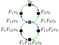
Figure 3. The action of $\overline{U}$ on the weight spaces of $V({\smash{\text{\boldmath{$t$}}}})$.

We now state the genericity condition on $V({\smash{\text{\boldmath{$t$}}}})$. Let

$$\mathcal{X}_{1} =\{{\smash{\text{\boldmath{$t$}}}}\in\mathcal{P}:t_{1}^{2}=1\}, \mathcal{X}_{2} =\{{\smash{\text{\boldmath{$t$}}}}\in\mathcal{P}:t_{2}^{2}=1\} \mathcal{X}_{12} =\{{\smash{\text{\boldmath{$t$}}}}\in\mathcal{P}:(t_{1}t_{2})^{2}=-1\},$$ (41)

then set $\mathcal{R}$ to be the union of $\mathcal{X}_{1}$, $\mathcal{X}_{2}$, and $\mathcal{X}_{12}$. We partition $\mathcal{R}$ into disjoint subsets indexed by nonempty subsets $I\subsetneq{\Phi^{+}}$, with

$$\mathcal{R}_{I}=\left(\bigcap_{\alpha\in I}\mathcal{X}_{\alpha}\right)\setminus\left(\bigcup_{\alpha\notin I}\mathcal{X}_{\alpha}\right)$$ (42)

Proposition 3.4 ([Har19b]).

The representation $V({\smash{\text{\boldmath{$t$}}}})$ of $\overline{U}$ is irreducible if and only if ${\smash{\text{\boldmath{$t$}}}}\notin\mathcal{R}$.

If $t$ belongs to $\mathcal{R}_{1}$, $\mathcal{R}_{2}$, or $\mathcal{R}_{12}$ then the socle of $V({\smash{\text{\boldmath{$t$}}}})$ is an irreducible subrepresentation of dimension four. Moreover, the head is four-dimensional, irreducible, and has highest weight $t$. We use $B_{i}$ to denote the subalgebra of $\overline{U}$ generated by $B$ and $F_{i}$.

3.3. The Representations $X({\smash{\text{\boldmath{$t$}}}})$ and $Y({\smash{\text{\boldmath{$t$}}}})$

We begin with ${\smash{\text{\boldmath{$t$}}}}\in\mathcal{X}_{1}$ and ${\smash{\text{\boldmath{$t$}}}}\in\mathcal{X}_{2}$ to define $X({\smash{\text{\boldmath{$t$}}}})$ and $Y({\smash{\text{\boldmath{$t$}}}})$, respectively.

Definition 3.5.

Suppose ${\smash{\text{\boldmath{$t$}}}}\in\mathcal{X}_{2}$. Let $\gamma_{{\smash{\text{\boldmath{$t$}}}}}^{X}$ be the extension of the character $\gamma_{{\smash{\text{\boldmath{$t$}}}}}$ on $B$ to $B_{2}$ with $\gamma_{{\smash{\text{\boldmath{$t$}}}}}^{X}(F_{2})=0$. Set $X_{{\smash{\text{\boldmath{$t$}}}}}=\langle x_{0}\rangle$ to be the one-dimensional $B_{2}$-module determined by $\gamma_{{\smash{\text{\boldmath{$t$}}}}}^{X}$ and define

$$X({\smash{\text{\boldmath{$t$}}}})={\text{{Ind}}_{B_{2}}^{\overline{U}}(X_{{\smash{\text{\boldmath{$t$}}}}})=\overline{U}\otimes_{B_{2}}X_{{\smash{\text{\boldmath{$t$}}}}}}.$$ (43)

The representation $Y({\smash{\text{\boldmath{$t$}}}})$ is defined analogously by assuming ${\smash{\text{\boldmath{$t$}}}}\in\mathcal{X}_{1}$ and setting the action of $F_{1}$ to be zero on the generating vector.

Remark 3.6.

The representation $X({\smash{\text{\boldmath{$t$}}}})$ is defined if and only if ${\smash{\text{\boldmath{$t$}}}}\in\mathcal{X}_{2}$. Observe that

$$0=[E_{2},F_{2}]x_{0}=\left\lfloor K_{2}\right\rfloor x_{0}=\left\lfloor t_{2}\right\rfloor x_{0}$$ (44)

if and only if $t_{2}^{2}=1$.

For each $\psi\in\Psi$, let ${\smash{\text{\boldmath{$\sigma^{\psi}$}}}}\in\mathcal{P}$ be the weight of $F^{\psi}v_{0}$ in $V(1,1)$.

Proposition 3.7.

If ${\smash{\text{\boldmath{$t$}}}}\in\mathcal{X}_{2}$ or ${\smash{\text{\boldmath{$t$}}}}\in\mathcal{X}_{1}$, we have the respective exact sequence

$$0\rightarrow X({\smash{\text{\boldmath{$\sigma^{(001)}$}}}}{\smash{\text{\boldmath{$t$}}}})\rightarrow V({\smash{\text{\boldmath{$t$}}}})\rightarrow X({\smash{\text{\boldmath{$t$}}}})\rightarrow 0$$ (45)

$$0\rightarrow Y({\smash{\text{\boldmath{$\sigma^{(100)}$}}}}{\smash{\text{\boldmath{$t$}}}})\rightarrow V({\smash{\text{\boldmath{$t$}}}})\rightarrow Y({\smash{\text{\boldmath{$t$}}}})\rightarrow 0.$$ (46)

As a subrepresentation of $V({\smash{\text{\boldmath{$t$}}}})$, $X({\smash{\text{\boldmath{$\sigma^{(001)}$}}}}{\smash{\text{\boldmath{$t$}}}})$ has a basis given by

$$\langle F^{(001)}v_{0},F^{(101)}v_{0},F^{(011)}v_{0},F^{(111)}v_{0}\rangle$$ (47)

and is indicated by the red points in Figure 4. The quotient representation is colored gray and the action of $F_{2}$ which vanishes under the identification is indicated by a dotted arrow. Moreover, assuming ${\smash{\text{\boldmath{$t$}}}}\in\mathcal{R}_{2}$ is equivalent to assuming both $X({\smash{\text{\boldmath{$\sigma^{(001)}$}}}}{\smash{\text{\boldmath{$t$}}}})$ and its quotient in $V({\smash{\text{\boldmath{$t$}}}})$ are irreducible. Analogous statements are true for $Y({\smash{\text{\boldmath{$\sigma^{(100)}$}}}}{\smash{\text{\boldmath{$t$}}}})$ by switching the indices 1 and 2.

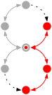
(a) ${\smash{\text{\boldmath{$t$}}}}\in\mathcal{R}_{2}$

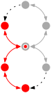
(b) ${\smash{\text{\boldmath{$t$}}}}\in\mathcal{R}_{1}$

Figure 4. Reducible $V({\smash{\text{\boldmath{$t$}}}})$ with subrepresentations $X({\smash{\text{\boldmath{$\sigma^{(001)}$}}}}{\smash{\text{\boldmath{$t$}}}})$ and $Y({\smash{\text{\boldmath{$\sigma^{(100)}$}}}}{\smash{\text{\boldmath{$t$}}}})$.

3.4. The Representation $W({\smash{\text{\boldmath{$t$}}}})$

Motivating the ${\smash{\text{\boldmath{$t$}}}}\in\mathcal{X}_{12}$ case, we consider a quotient of $V({\smash{\text{\boldmath{$t$}}}})$ so that there is a linear dependence between $F_{1}F_{2}v_{0}$ and $F_{2}F_{1}v_{0}$, i.e. $F_{1}F_{2}v_{0}-\alpha F_{2}F_{1}v_{0}=0$ for some $\alpha\in\mathbb{Q}(\zeta,t)$. Then

$$E_{1}(F_{1}F_{2}v_{0}-\alpha F_{2}F_{1}v_{0})=0, E_{2}(F_{1}F_{2}v_{0}-\alpha F_{2}F_{1}v_{0})=0,$$ (48)

and together imply $\alpha=\dfrac{\left\lfloor\zeta t_{1}\right\rfloor}{\left\lfloor t_{1}\right\rfloor}=\dfrac{\left\lfloor t_{2}\right\rfloor}{\left\lfloor\zeta t_{2}\right\rfloor}$. These equalities involving $\alpha$ are true if and only if $t_{1}^{2}t_{2}^{2}=-1$ and $t_{1}^{2}\neq 1$. Therefore, we set

$$B_{12}=\langle B,F_{1}F_{2}\left\lfloor K_{1}\right\rfloor-F_{2}F_{1}\left\lfloor\zeta K_{1}\right\rfloor\rangle$$ (49)

and let $\gamma_{{\smash{\text{\boldmath{$t$}}}}}^{W}$ be the character on $B_{12}$ which is an extension of $\gamma_{{\smash{\text{\boldmath{$t$}}}}}$ on $B$ and is zero otherwise.

Definition 3.8.

Let ${\smash{\text{\boldmath{$t$}}}}\in\mathcal{X}_{12}$ and let $W_{{\smash{\text{\boldmath{$t$}}}}}=\langle w_{0}\rangle$ be the one-dimensional $B_{12}$-module determined by $\gamma_{{\smash{\text{\boldmath{$t$}}}}}^{W}$. We define $W({\smash{\text{\boldmath{$t$}}}})$ by induction

$$W({\smash{\text{\boldmath{$t$}}}})=\text{Ind}_{B_{12}}^{\overline{U}}(W_{{\smash{\text{\boldmath{$t$}}}}})=\overline{U}\otimes_{B_{12}}W_{{\smash{\text{\boldmath{$t$}}}}}.$$ (50)

Remark 3.9.

To define $W({\smash{\text{\boldmath{$t$}}}})$, we require ${\smash{\text{\boldmath{$t$}}}}\in\mathcal{X}_{12}$ so that $E_{2}.(F_{1}F_{2}\left\lfloor K_{1}\right\rfloor-F_{2}F_{1}\left\lfloor\zeta K_{1}\right\rfloor)w_{0}$ vanishes. The dependence between $F_{1}F_{2}w_{0}$ and $F_{2}F_{1}w_{0}$ imply that $W({\smash{\text{\boldmath{$t$}}}})$ is four dimensional.

We define an inclusion of $W({\smash{\text{\boldmath{$\sigma^{(010)}$}}}}{\smash{\text{\boldmath{$t$}}}})$ in $V({\smash{\text{\boldmath{$t$}}}})$ by sending $w_{0}$ to $\left(\left\lfloor t_{1}\right\rfloor F_{1}F_{2}-\left\lfloor\zeta t_{1}\right\rfloor F_{2}F_{1}\right)v_{0}$ and extending equivariantly. Quotienting out $W({\smash{\text{\boldmath{$\sigma^{(010)}$}}}}{\smash{\text{\boldmath{$t$}}}})$ returns us to the situation described in the motivation of this case.

Proposition 3.10.

If ${\smash{\text{\boldmath{$t$}}}}\in\mathcal{X}_{12}$, we have the following exact sequence:

$$0\rightarrow W({\smash{\text{\boldmath{$\sigma^{(010)}$}}}}{\smash{\text{\boldmath{$t$}}}})\rightarrow V({\smash{\text{\boldmath{$t$}}}})\rightarrow W({\smash{\text{\boldmath{$t$}}}})\rightarrow 0.$$ (51)

In Figure 5, we assume ${\smash{\text{\boldmath{$t$}}}}\in\mathcal{R}_{12}$ so that both $W({\smash{\text{\boldmath{$t$}}}})$ and $W({\smash{\text{\boldmath{$\sigma^{(010)}$}}}}{\smash{\text{\boldmath{$t$}}}})$ are irreducible. Again, the subrepresentation is colored red and the resulting quotient is gray. Unlike Figure 4, the trivialized actions of $F_{1}$ and $F_{2}$ are not indicated by dotted arrows because the lowest weight of $W({\smash{\text{\boldmath{$t$}}}})$ is the same as the highest weight of $W({\smash{\text{\boldmath{$\sigma^{(010)}$}}}}{\smash{\text{\boldmath{$t$}}}})$, and both $F_{1}$ and $F_{2}$ act non-trivially on this weight space in the subrepresentation.

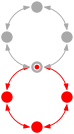
(a) ${\smash{\text{\boldmath{$t$}}}}\in\mathcal{R}_{12}$

Figure 5. Reducible $V({\smash{\text{\boldmath{$t$}}}})$ with subrepresentation $W({\smash{\text{\boldmath{$\sigma^{(010)}$}}}}{\smash{\text{\boldmath{$t$}}}})$.

3.5. Tensor Decompositions Involving Irreducible Subrepresentations

We state two theorems on tensor decompositions of $V({\smash{\text{\boldmath{$t$}}}})$, $X({\smash{\text{\boldmath{$t$}}}})$, $Y({\smash{\text{\boldmath{$t$}}}})$, and $W({\smash{\text{\boldmath{$t$}}}})$ for sufficiently generic parameters.

Proof.

To establish the isomorphism (8), we consider the module homomorphism

$$f:V({\smash{\text{\boldmath{$t$}}}}{\smash{\text{\boldmath{$s$}}}})\oplus V({\smash{\text{\boldmath{$\sigma^{(110)}$}}}}{\smash{\text{\boldmath{$t$}}}}{\smash{\text{\boldmath{$s$}}}})\oplus V({\smash{\text{\boldmath{$\sigma^{(100)}$}}}}{\smash{\text{\boldmath{$t$}}}}{\smash{\text{\boldmath{$s$}}}})\rightarrow X({\smash{\text{\boldmath{$t$}}}})\otimes X({\smash{\text{\boldmath{$s$}}}})$$

completely determined by the image of the highest weight vectors of $V({\smash{\text{\boldmath{$t$}}}}{\smash{\text{\boldmath{$s$}}}})$, $V({\smash{\text{\boldmath{$\sigma^{(110)}$}}}}{\smash{\text{\boldmath{$t$}}}}{\smash{\text{\boldmath{$s$}}}})$, and $V({\smash{\text{\boldmath{$\sigma^{(100)}$}}}}{\smash{\text{\boldmath{$t$}}}}{\smash{\text{\boldmath{$s$}}}})$. We define the respective highest weight vectors in the image of $f$ to be:

$$x_{0}\otimes x_{0}, \Delta(E_{1}E_{2}E_{1}).(F_{1}F_{2}F_{1}x_{0}\otimes F_{1}F_{2}F_{1}x_{0}), \Delta(E_{1}).(F_{1}x_{0}\otimes F_{1}x_{0}).$$ and (52)

Note that these have the correct weights. By assumption ${\smash{\text{\boldmath{$\sigma^{(110)}$}}}}{\smash{\text{\boldmath{$t$}}}}{\smash{\text{\boldmath{$s$}}}},{\smash{\text{\boldmath{$\sigma^{(100)}$}}}}{\smash{\text{\boldmath{$t$}}}}{\smash{\text{\boldmath{$s$}}}}\notin\mathcal{R}_{1}\cup\mathcal{R}_{12}$, thus these vectors are nonzero and have distinct weights. By Proposition 3.7 and the remark following it, $V({\smash{\text{\boldmath{$t$}}}}{\smash{\text{\boldmath{$s$}}}})$ and $V({\smash{\text{\boldmath{$\sigma^{(110)}$}}}}{\smash{\text{\boldmath{$t$}}}}{\smash{\text{\boldmath{$s$}}}})$ are reducible, but their heads are irreducible and have highest weights $t$$s$ and $\sigma^{(110)}$$t$$s$ respectively. We also have that $V({\smash{\text{\boldmath{$\sigma^{(100)}$}}}}{\smash{\text{\boldmath{$t$}}}}{\smash{\text{\boldmath{$s$}}}})$ is irreducible by assumption. Thus, the head of each of $V({\smash{\text{\boldmath{$t$}}}}{\smash{\text{\boldmath{$s$}}}})$, $V({\smash{\text{\boldmath{$\sigma^{(110)}$}}}}{\smash{\text{\boldmath{$t$}}}}{\smash{\text{\boldmath{$s$}}}})$, and $V({\smash{\text{\boldmath{$\sigma^{(100)}$}}}}{\smash{\text{\boldmath{$t$}}}}{\smash{\text{\boldmath{$s$}}}})$ is mapped to distinct nonzero subspaces under $f$. The socles of $V({\smash{\text{\boldmath{$t$}}}}{\smash{\text{\boldmath{$s$}}}})$ and $V({\smash{\text{\boldmath{$\sigma^{(110)}$}}}}{\smash{\text{\boldmath{$t$}}}}{\smash{\text{\boldmath{$s$}}}})$ are irreducible and have highest weights $\sigma^{(001)}$$t$$s$ and $-ts$. Therefore, they must belong to $\ker{f}$. Quotienting out this kernel yields the desired isomorphism.

We have a similar construction for (9), with the highest weight vectors given by exchanging indices 1 and 2 from (52). In the $W({\smash{\text{\boldmath{$t$}}}})\otimes W({\smash{\text{\boldmath{$s$}}}})$ case, the respective generating vectors are

$$\Delta(E_{1}).(F_{1}w_{0}\otimes F_{1}w_{0}), \Delta(E_{2}).(F_{2}w_{0}\otimes F_{2}w_{0}) w_{0}\otimes w_{0}.$$ and

∎

Although we will not use them in this paper, we include the data of mixed tensor products for completeness.

Theorem 3.11 (Mixed Tensor Decomposition).

For each isomorphism below, we assume ${\smash{\text{\boldmath{$t$}}}},{\smash{\text{\boldmath{$s$}}}}\in\mathcal{P}$ are chosen so that the four-dimensional representations which appear are well-defined and all summands are irreducible:

$$X({\smash{\text{\boldmath{$t$}}}})\otimes Y({\smash{\text{\boldmath{$s$}}}}) \cong V({\smash{\text{\boldmath{$ts$}}}})\oplus V({\smash{\text{\boldmath{$\sigma^{(010)}$}}}}{\smash{\text{\boldmath{$ts$}}}})$$ (53)

$$X({\smash{\text{\boldmath{$t$}}}})\otimes W({\smash{\text{\boldmath{$s$}}}}) \cong V({\smash{\text{\boldmath{$ts$}}}})\oplus V({\smash{\text{\boldmath{$\sigma^{(100)}$}}}}{\smash{\text{\boldmath{$ts$}}}})$$ (54)

$$Y({\smash{\text{\boldmath{$t$}}}})\otimes W({\smash{\text{\boldmath{$s$}}}}) \cong V({\smash{\text{\boldmath{$ts$}}}})\oplus V({\smash{\text{\boldmath{$\sigma^{(001)}$}}}}{\smash{\text{\boldmath{$ts$}}}})$$ (55)

$$V({\smash{\text{\boldmath{$t$}}}})\otimes X({\smash{\text{\boldmath{$s$}}}})\cong V({\smash{\text{\boldmath{$t$}}}}{\smash{\text{\boldmath{$s$}}}}) \oplus V({\smash{\text{\boldmath{$\sigma^{(100)}$}}}}{\smash{\text{\boldmath{$t$}}}}{\smash{\text{\boldmath{$s$}}}})\oplus V({\smash{\text{\boldmath{$\sigma^{(010)}$}}}}{\smash{\text{\boldmath{$t$}}}}{\smash{\text{\boldmath{$s$}}}})\oplus V({\smash{\text{\boldmath{$\sigma^{(110)}$}}}}{\smash{\text{\boldmath{$ts$}}}})$$ (56)

$$V({\smash{\text{\boldmath{$t$}}}})\otimes Y({\smash{\text{\boldmath{$s$}}}})\cong V({\smash{\text{\boldmath{$t$}}}}{\smash{\text{\boldmath{$s$}}}}) \oplus V({\smash{\text{\boldmath{$\sigma^{(001)}$}}}}{\smash{\text{\boldmath{$t$}}}}{\smash{\text{\boldmath{$s$}}}})\oplus V({\smash{\text{\boldmath{$\sigma^{(010)}$}}}}{\smash{\text{\boldmath{$t$}}}}{\smash{\text{\boldmath{$s$}}}})\oplus V({\smash{\text{\boldmath{$\sigma^{(011)}$}}}}{\smash{\text{\boldmath{$ts$}}}})$$ (57)

$$V({\smash{\text{\boldmath{$t$}}}})\otimes W({\smash{\text{\boldmath{$s$}}}})\cong V({\smash{\text{\boldmath{$t$}}}}{\smash{\text{\boldmath{$s$}}}}) \oplus V({\smash{\text{\boldmath{$\sigma^{(100)}$}}}}{\smash{\text{\boldmath{$t$}}}}{\smash{\text{\boldmath{$s$}}}})\oplus V({\smash{\text{\boldmath{$\sigma^{(001)}$}}}}{\smash{\text{\boldmath{$t$}}}}{\smash{\text{\boldmath{$s$}}}})\oplus V({\smash{\text{\boldmath{$\sigma^{(010)}$}}}}{\smash{\text{\boldmath{$t$}}}}{\smash{\text{\boldmath{$s$}}}}).$$ (58)

Proof.

Using the same argument as above, we only provide highest weight vectors which generate an irreducible representation under the action of $F_{1}$ and $F_{2}$. We then check the weights of these generating vectors, which indicate the isomorphism class of the resulting representation. We omit cases below involving $Y({\smash{\text{\boldmath{$t$}}}})$ when the result can be determined from the expression for $X({\smash{\text{\boldmath{$t$}}}})$ by switching the indices $1$ and $2$.

$\begin{array}[]{cc}X({\smash{\text{\boldmath{$t$}}}})\otimes Y({\smash{\text{\boldmath{$s$}}}}):&x_{0}\otimes y_{0},\Delta(E_{1}E_{2}E_{1}E_{2}).(F_{1}F_{2}F_{1}x_{0}\otimes F_{2}F_{1}F_{2}y_{0})\\ X({\smash{\text{\boldmath{$t$}}}})\otimes W({\smash{\text{\boldmath{$s$}}}}):&x_{0}\otimes w_{0},\Delta(E_{1}).(F_{1}x_{0}\otimes F_{1}w_{0})\\ V({\smash{\text{\boldmath{$t$}}}})\otimes X({\smash{\text{\boldmath{$s$}}}}):&v_{0}\otimes x_{0},\Delta(E_{1})(F_{1}v_{0}\otimes F_{1}x_{0}),\Delta(E_{1}E_{2}E_{1}E_{2})(F_{1}F_{2}F_{1}v_{0}\otimes F_{2}F_{1}F_{2}x_{0}),\\ &\Delta(E_{1}E_{2}E_{1}E_{2})(F_{1}F_{2}F_{1}v_{0}\otimes F_{1}F_{2}F_{1}F_{2}x_{0})\\ V({\smash{\text{\boldmath{$t$}}}})\otimes W({\smash{\text{\boldmath{$s$}}}}):&v_{0}\otimes w_{0},\Delta(E_{1}).(F_{1}v_{0}\otimes F_{1}w_{0}),\Delta(E_{2}).(F_{2}v_{0}\otimes F_{2}w_{0}),\\ &\Delta(E_{1}E_{2}E_{1}E_{2}).(F_{1}F_{2}v_{0}\otimes F_{1}F_{2}F_{1}F_{2}w_{0})\end{array}$

∎

4. Unrolled Restricted Quantum Groups and Braiding

We begin this section by recalling the unrolled restricted quantum group in Definition 4.2. According to [GP13], at odd roots of unity, its category of weight representations admits a braiding c. We show directly that there is a braiding for $\mathfrak{g}=\mathfrak{sl}_{3}$ at a primitive fourth root of unity using the notion of standard pre-triangular based on the work of [CP95, Tan92]. We introduce the pivotal structure in this category in Subsection 4.2 and also provide a renormalization of the braiding that removes the dependence on the $H_{i}$-weights $\lambda$ up to exponentiation. We end this section with the renormalized action for quantum $\mathfrak{sl}_{3}$ on the tensor decomposition of $V({\smash{\text{\boldmath{$t$}}}})\otimes V({\smash{\text{\boldmath{$t$}}}})$ in Corollary 4.12.

Convention 4.1.

Throughout this section, we assume $\overline{U}_{\zeta}(\mathfrak{g})$ is a SQHA.

Definition 4.2.

Let $\mathfrak{g}$ be a semisimple Lie algebra of rank $n$. We define unrolled restricted quantum $\mathfrak{g}$ at a fourth root of unity $\overline{U}^{H}_{\zeta}(\mathfrak{g})$, also denoted $\overline{U}^{H}$, to be the algebra $\overline{U}_{\zeta}(\mathfrak{g})[H_{1},\dots,H_{n}]$ with relations:

$$H_{i}K_{j}^{\pm}=K_{j}^{\pm}H_{i}, [H_{i},E_{j}]=A_{ij}E_{j}, [H_{i},F_{j}]=-A_{ij}F_{j},$$ (59)

in addition to the relations of $\overline{U}_{\zeta}(\mathfrak{g})$ itself.

The representation $V({\smash{\text{\boldmath{$t$}}}})$ extends from the restricted quantum group to the unrolled restricted quantum group as follows.

Definition 4.3.

Fix a character ${\smash{\text{\boldmath{$t$}}}}\in\mathcal{P}$. Choose ${\smash{\text{\boldmath{$\lambda$}}}}=(\lambda_{1},\dots,\lambda_{n})\in\mathbb{C}^{n}$ such that $\zeta^{{d}\cdot{\smash{\text{\boldmath{$\lambda$}}}}}={\smash{\text{\boldmath{$t$}}}}$, by which we mean $\zeta^{d_{i}\lambda_{i}}=e^{d_{i}\pi i\lambda_{i}/2}=t_{i}$ for each $i\in\{1,\dots,n\}$. We define $V^{H}({\smash{\text{\boldmath{$\lambda$}}}})$ to be the $\overline{U}^{H}_{\zeta}(\mathfrak{g})$ representation which restricts to $V({\smash{\text{\boldmath{$t$}}}})$ on $\overline{U}_{\zeta}(\mathfrak{g})$ and $H_{i}v_{0}=\lambda_{i}v_{0}$ for each $i\in\{1,\dots,n\}$.

Since $t_{i}\neq 0$ there are infinitely many isomorphism classes of representations $V^{H}({\smash{\text{\boldmath{$\lambda$}}}})$ that restrict to the same $V({\smash{\text{\boldmath{$t$}}}})$. In Proposition 4.10, we prove that the $R$-matrix action on $V^{H}({\smash{\text{\boldmath{$\lambda$}}}})\otimes V^{H}({\smash{\text{\boldmath{$\lambda$}}}})$, when properly normalized, depends only on ${\smash{\text{\boldmath{$t$}}}}=\zeta^{d\cdot{\smash{\text{\boldmath{$\lambda$}}}}}$.

We say that a $\overline{U}^{H}_{\zeta}(\mathfrak{g})$-module $V$ is a weight module if $V$ is a direct sum of weight spaces, the actions of $H_{1},\dots,H_{n}$ are diagonal, and $H_{i}v_{0}=\lambda_{i}v_{0}$ implies $K_{i}v_{0}=\zeta^{d_{i}\lambda_{i}}v_{0}$. Let $\overline{U}^{H}\operatorname{-wmod}$ denote the category of $\overline{U}^{H}$-weight modules. The objects of $\overline{U}^{H}\operatorname{-wmod}$ are pairs $(V,\rho)$ where $V$ is a vector space and $\rho:\overline{U}^{H}\to\operatorname{End}{(V)}$ is a homomorphism. The category $\overline{U}\operatorname{-wmod}$ of $\overline{U}$-weight modules is obtained from $\overline{U}^{H}\operatorname{-wmod}$ by forgetting the actions of $H_{1},\dots,H_{n}$.

4.1. The $R$-matrix

A formula for the $R$-matrix as an operator on representations of unrolled quantum (super) groups at odd roots of unity is given in [GP13, AGP21]. The formula naturally extends to general roots of unity as stated in [CR21, Rup20]. We show by direct computation that the expression in (63) satisfies the quasi $R$-matrix relations for $\mathfrak{g}=\mathfrak{sl}_{3}$.

For each pair of representations $(V,\rho),(W,\rho^{\prime})\in\overline{U}^{H}\operatorname{-wmod}$, we define an automorphism $E_{\rho,\rho^{\prime}}$ as follows. Let $v\in V$ and $w\in W$ be weight vectors such that $H_{i}v=\mu_{i}v$ and $H_{j}w=\nu_{j}w$, then

$$E_{\rho,\rho^{\prime}}(v\otimes w)=\zeta^{{\sum_{ij}d_{i}(A^{-1})_{ij}\mu_{i}\nu_{j}}}(v\otimes w).$$ (60)

Thus, $E_{\rho,\rho^{\prime}}$ can be thought of as the formal expression $\zeta^{{\sum_{ij}d_{i}(A^{-1})_{ij}H_{i}\otimes H_{j}}}$, which can also be defined as a power series.

Let $\Psi_{\zeta}$ be the automorphism of $\overline{U}^{H}\otimes\overline{U}^{H}$ defined so that for all $x,y\in\overline{U}^{H}$ of weights $\alpha$ and $\beta$, respectively:

$$\Psi_{\zeta}(x\otimes y)=\zeta^{-\langle\alpha,\beta\rangle}(xK_{\beta}^{-1}\otimes yK_{\alpha}^{-1}).$$ (61)

This automorphism is a specialization of $\Psi_{q}$ defined in [CP95, Tan92] to $q=\zeta$ which acts on the unrolled restricted quantum group, also see [GP13, Lemma 40]. Similarly, $E_{\rho,\rho^{\prime}}$ is defined for generic $q$ in [CP95]. However, we use the same notation here to mean the specialization to $q=\zeta$ acting on tensor product representations in $\overline{U}^{H}_{\zeta}(\mathfrak{g})\operatorname{-wmod}$. By the same computations given in [CP95, Proposition 10.1.19], $E_{\rho,\rho^{\prime}}$ implements $\Psi_{\zeta}$ on tensor products of weight representations in the sense that for all $x,y\in\overline{U}^{H}_{\zeta}(\mathfrak{g})$ the following relation holds:

$$(\rho\otimes\rho^{\prime})(\Psi_{\zeta}(x\otimes y))=E_{\rho,\rho^{\prime}}^{-1}(\rho(x)\otimes\rho^{\prime}(y))E_{\rho,\rho^{\prime}}.$$ (62)

Definition 4.4.

An element $R\in\overline{U}_{\zeta}^{H}(\mathfrak{g})\otimes\overline{U}_{\zeta}^{H}(\mathfrak{g})$ satisfying the following relations is called a quasi $R$-matrix:

$${R}\text{ is invertible,} {R}\Delta(x)=\Psi_{\zeta}(\Delta^{op}(x)){R}\text{ for all }x\in\overline{U}_{\zeta}^{H}(\mathfrak{g}),$$

$$(\Psi_{\zeta})_{23}({R}_{13}){R}_{23}=(\Delta\otimes 1)({R}), (\Psi_{\zeta})_{12}({R}_{13}){R}_{12}=(1\otimes\Delta)({R}).$$

For each $\mathfrak{g}$, set

$$\check{R}=\prod_{\beta\in\overline{{\Phi^{+}}}}(1\otimes 1+(\zeta_{\beta}-\zeta^{-1}_{\beta})E_{\beta}\otimes F_{\beta})\in\overline{U}_{\zeta}^{H}(\mathfrak{g})\otimes\overline{U}_{\zeta}^{H}(\mathfrak{g}).$$ (63)

We say $\overline{U}_{\zeta}^{H}(\mathfrak{g})$ is standard pre-triangular if $\check{R}$ is a quasi $R$-matrix.

Proposition 4.5.

Let $\overline{U}^{H}$ be a standard pre-triangular quantum group. Suppose $(V,\rho),(W,\rho^{\prime})\in\overline{U}^{H}\operatorname{-wmod}$ and define

$$\textit{{c}}_{V,W}=P\circ E_{\rho,\rho^{\prime}}(\rho\otimes\rho^{\prime})(\check{R})\in\operatorname{Hom}_{\overline{U}^{H}}(V\otimes W,W\otimes V).$$ (64)

Here $E_{\rho,\rho^{\prime}}$ and $(\rho\otimes\rho^{\prime})(\check{R})$, defined above, act as a linear maps on tensor product representations, and $P$ is the tensor swap. Then $\overline{U}^{H}\operatorname{-wmod}$ is a braided monoidal category with braiding $\textit{{c}}=\{\textit{{c}}_{V,W}:V,W\in\overline{U}^{H}\operatorname{-wmod}\}$.

Proof.

Fix representations $(V,\rho),(W,\rho^{\prime}),(U,\rho^{\prime\prime})\in\overline{U}^{H}\operatorname{-wmod}$. To prove that c is a braiding, we show that $\textit{{c}}_{V,W}$ is an invertible morphism in $\overline{U}^{H}\operatorname{-wmod}$ and satisfies the hexagon (triangle) identities:

$$(\textit{{c}}_{V,U}\otimes id_{W})\circ(id_{V}\otimes\textit{{c}}_{W,U})=\textit{{c}}_{V\otimes W,U} (id_{W}\otimes\textit{{c}}_{V,U})\circ(\textit{{c}}_{V,W}\otimes id_{U})=\textit{{c}}_{V,W\otimes U}.$$

We prove $\textit{{c}}_{V,W}$ is a morphism in $\overline{U}^{H}\operatorname{-wmod}$ by showing it intertwines the action of arbitrary $x\in\overline{U}^{H}$. Pre-triangularity implies

$$E_{\rho,\rho^{\prime}}(\rho\otimes\rho^{\prime})(\check{R}\Delta(x))=(\rho\otimes\rho^{\prime})(\Delta^{op}(x))E_{\rho,\rho^{\prime}}(\rho\otimes\rho^{\prime})(\check{R}).$$

Thus,

$$\textit{{c}}_{V,W}(\rho\otimes\rho^{\prime})(\Delta(x)) =P\circ E_{\rho,\rho^{\prime}}(\rho\otimes\rho^{\prime})(\check{R}\Delta(x))$$

$$=P\circ(\rho\otimes\rho^{\prime})(\Delta^{op}(x))E_{\rho,\rho^{\prime}}(\rho\otimes\rho^{\prime})(\check{R})$$

$$=(\rho\otimes\rho^{\prime})(\Delta(x))P\circ E_{\rho,\rho^{\prime}}(\rho\otimes\rho^{\prime})(\check{R})$$

$$=(\rho\otimes\rho^{\prime})(\Delta(x))\textit{{c}}_{V,W}.$$

Since $\check{R}$ is invertible, $\textit{{c}}_{V,W}$ is an isomorphism with inverse

$$\textit{{c}}_{V,W}^{-1}=\left(\prod_{\beta\in\overline{{\Phi^{+}}}}^{reverse}(1\otimes 1-(\zeta_{\beta}-\zeta_{\beta}^{-1})E_{\beta}\otimes F_{\beta})E_{\rho,\rho^{\prime}}^{-1}\right)\circ P,$$

with $\prod_{\alpha\in\overline{{\Phi^{+}}}}^{reverse}$ indicating the product follows the opposite ordering on $\overline{{\Phi^{+}}}$.

We now prove the first hexagon (triangle) relation, and the second follows a similar argument. By the latter standard pre-triangular axioms,

$$(\textit{{c}}_{V,U}\otimes id_{W})\circ(id_{V}\otimes\textit{{c}}_{W,U}) =P_{12}\circ(E_{\rho,\rho^{\prime\prime}})_{12}(\rho\otimes\rho^{\prime\prime}\otimes\rho^{\prime})(\check{R}_{12})\circ P_{23}\circ(E_{\rho^{\prime},\rho^{\prime\prime}})_{23}(\rho\otimes\rho^{\prime}\otimes\rho^{\prime\prime})(\check{R}_{23})$$

$$=P_{12}P_{23}\circ(E_{\rho,\rho^{\prime\prime}})_{13}(\rho\otimes\rho^{\prime}\otimes\rho^{\prime\prime})(\check{R}_{13})(E_{\rho^{\prime},\rho^{\prime\prime}})_{23}(\rho\otimes\rho^{\prime}\otimes\rho^{\prime\prime})(\check{R}_{23})$$

$$=P_{12,3}\circ(E_{\rho,\rho^{\prime\prime}})_{13}(E_{\rho^{\prime},\rho^{\prime\prime}})_{23}(\rho\otimes\rho^{\prime}\otimes\rho^{\prime\prime})\left((\Psi_{\zeta})_{23}(\check{R}_{13})\check{R}_{23}\right)$$

$$=P_{12,3}\circ(E_{\rho\otimes\rho^{\prime},\rho^{\prime\prime}})((\rho\otimes\rho^{\prime})\otimes\rho^{\prime\prime})\left((\Delta\otimes 1)(\check{R})\right)$$

$$=\textit{{c}}_{V,W\otimes U}.$$

∎

Remark 4.6.

It is straightforward to verify that the braiding also satisfies the quantum Yang-Baxter equation.

Just as in our discussion regarding the Hopf algebra structure on $\overline{U}_{\zeta}(\mathfrak{g})$, a careful analysis of the quasi $R$-matrix in the universal algebra $\overline{U}^{H}_{\zeta}(\mathfrak{g})$ is not available in the current literature. The pre-triangular properties of the truncated quasi $R$-matrix (63) were also considered in [AGP21, GP13], but proposed derivations lack formal details and, in fact, contain formulae, such as equation (46) in the proof of [GP13, Theorem 41], that are not true in the stated universal form. In Proposition 4.7, we verify the pre-triangular axioms for the $\overline{U}^{H}_{\zeta}(\mathfrak{sl}_{3})$ quasi $R$-matrix by explicit computations.

Proposition 4.7.

The quantum group $\overline{U}_{\zeta}^{H}(\mathfrak{sl}_{3})$ is standard pre-triangular.

Proof.

We prove that $\overline{U}^{H}_{\zeta}(\mathfrak{sl}_{3})$ is standard pre-triangular by showing $\check{R}\Delta(x)=\Psi_{\zeta}(\Delta^{op}(x))\check{R}$ for all $x\in\overline{U}^{H}_{\zeta}(\mathfrak{sl}_{3})$ and $(\Psi_{\zeta})_{23}(\check{R}_{13})\check{R}_{23}=(\Delta\otimes 1)(\check{R})$ both hold, the other conditions are readily verified.

To check $\check{R}\Delta(x)=\Psi_{\zeta}(\Delta^{op}(x))\check{R}$, we first note that $K_{i}$ and $H_{i}$ have symmetric coproducts which are preserved by $\Psi_{\zeta}$ and commute with $\check{R}$. Taking $x=E_{1}$ with $\Delta(E_{1})=E_{1}\otimes K_{1}+1\otimes E_{1}$, we verify that

$$\check{R}\Delta(E_{1})=\Psi_{\zeta}(\Delta^{op}(E_{1}))\check{R}=(E_{1}\otimes K_{1}^{-1}+1\otimes E_{1})\check{R}.$$

Computing each term of $\check{R}\Delta(E_{1})$ directly yields

$$\check{R}(E_{1}\otimes K_{1})=(1+2\zeta E_{1}\otimes F_{1})(1+2\zeta E_{12}\otimes F_{12})(E_{1}\otimes 1+2\zeta(\zeta E_{1}E_{2}+\zeta E_{12})\otimes F_{2})(1\otimes K_{1})$$

$$=(E_{1}\otimes 1)(1+2\zeta(-\zeta E_{12})\otimes F_{12})(1-2E_{2}\otimes F_{2})(1\otimes K_{1})+(1+2\zeta E_{1}\otimes F_{1})(-2E_{12}\otimes F_{2})(1\otimes K_{1})$$

$$=(E_{1}\otimes 1)(1+2E_{12}\otimes F_{12})(1-2E_{2}\otimes F_{2})(1\otimes K_{1})+(1\otimes K_{1})(1-2\zeta E_{1}\otimes F_{1})(2\zeta E_{12}\otimes F_{2})$$

$$=(E_{1}\otimes K_{1})(1+2\zeta E_{12}\otimes F_{12})(1+2\zeta E_{2}\otimes F_{2})+(1\otimes K_{1})(1-2\zeta E_{1}\otimes F_{1})(2\zeta E_{12}\otimes F_{2})$$

and

$$\check{R}(1\otimes E_{1})=(1+2\zeta E_{1}\otimes F_{1})(1+2\zeta E_{12}\otimes(E_{1}F_{12}-\zeta F_{2}K_{1}))(1+2\zeta E_{2}\otimes F_{2})$$

$$=(1\otimes E_{1})\check{R}+(-2\zeta E_{1}\otimes\left\lfloor K_{1}\right\rfloor)(1+2\zeta E_{12}\otimes F_{12})(1+2\zeta E_{2}\otimes F_{2})$$

$$+(1+2\zeta E_{1}\otimes F_{1})(2E_{12}\otimes F_{2}K_{1})$$

$$=(1\otimes E_{1})\check{R}+(-E_{1}\otimes(K_{1}-K_{1}^{-1}))(1+2\zeta E_{12}\otimes F_{12})(1+2\zeta E_{2}\otimes F_{2})$$

$$+(1\otimes K_{1})(1-2\zeta E_{1}\otimes F_{1})(-2\zeta E_{12}\otimes F_{2}).$$

Thus,

$$\check{R}(E_{1}\otimes K_{1}+1\otimes E_{1})=(1\otimes E_{1})\check{R}+(E_{1}\otimes K_{1}^{-1})(1+2\zeta E_{12}\otimes F_{12})(1+2\zeta E_{2}\otimes F_{2})$$

$$=(E_{1}\otimes K_{1}^{-1}+1\otimes E_{1})\check{R}.$$

The computation is similar for the other simple root generators, and so the relation holds for all $x\in\overline{U}^{H}_{\zeta}(\mathfrak{sl}_{3})$.

To prove the next condition, we observe

$$(\Psi_{\zeta})_{23}(\check{R}_{13})\check{R}_{23}=\prod_{\beta\in\overline{{\Phi^{+}}}}(1+2\zeta E_{\beta}\otimes K_{\beta}\otimes F_{\beta})\prod_{\beta\in\overline{{\Phi^{+}}}}(1+2\zeta\otimes E_{\beta}\otimes F_{\beta}).$$

For simple roots $\alpha$,

$$(1+2\zeta E_{\alpha}\otimes K_{\alpha}\otimes F_{\alpha})(1+2\zeta\otimes E_{\alpha}\otimes F_{\alpha})=(\Delta\otimes 1)(1+2\zeta E_{\alpha}\otimes F_{\alpha})$$

and for $\alpha=\alpha_{12}$,

$$(1+2\zeta E_{\alpha}\otimes K_{\alpha}\otimes F_{\alpha})(1+2\zeta 1\otimes E_{\alpha}\otimes F_{\alpha})$$

$$=(\Delta\otimes 1)(1+2\zeta E_{\alpha}\otimes F_{\alpha})+4\zeta E_{2}\otimes E_{1}K_{2}\otimes F_{12}.$$

We commute the terms appearing in $(\Psi_{\zeta})_{23}(\check{R}_{13})\check{R}_{23}$ so that the above product expressions for the coproduct appear and simplify to $(\Delta\otimes 1)(\check{R})$. The following equalities are readily verified:

$$[1+2\zeta E_{2}\otimes K_{2}\otimes F_{2} ,1+2\zeta\otimes E_{1}\otimes F_{1}]=-4\zeta E_{2}\otimes E_{1}K_{2}\otimes F_{12}$$

$$[1+2\zeta E_{12}\otimes K_{1}K_{2}\otimes F_{12} ,1+2\zeta\otimes E_{1}\otimes F_{1}]=0$$

$$[1+2\zeta E_{2}\otimes K_{2}\otimes F_{2} ,1+2\zeta\otimes E_{12}\otimes F_{12}]=0.$$

Thus,

$$\Psi_{\zeta,23}(\check{R}_{13})\check{R}_{23}=\prod_{\beta\in\overline{{\Phi^{+}}}}(1^{\otimes 3}+2\zeta E_{\beta}\otimes K_{\beta}\otimes F_{\beta})\prod_{\beta\in\overline{{\Phi^{+}}}}(1^{\otimes 3}+2\zeta\otimes E_{\beta}\otimes F_{\beta})$$

$$=\prod_{\beta\in\{1,12\}}(1+2\zeta E_{\beta}\otimes K_{\beta}\otimes F_{\beta})$$

$$\cdot\left((1+2\zeta\otimes E_{1}\otimes F_{1})(1+2\zeta E_{2}\otimes K_{2}\otimes F_{2})-4\zeta E_{2}\otimes E_{1}K_{2}\otimes F_{12}\right)\prod_{\alpha\in\{12,2\}}(1+2\zeta\otimes E_{\beta}\otimes F_{\beta})$$

$$=(\Delta\otimes 1)(1+2\zeta E_{1}\otimes F_{1})\left((\Delta\otimes 1)(1+2\zeta E_{12}\otimes F_{12})+4\zeta E_{2}\otimes E_{1}K_{2}\otimes F_{12}\right)$$

$$\cdot(\Delta\otimes id)(1+2\zeta E_{2}\otimes F_{2})-4\zeta(1+2\zeta E_{1}\otimes K_{1}\otimes F_{1})(E_{2}\otimes E_{1}K_{2}\otimes F_{12})(1+2\zeta\otimes E_{2}\otimes F_{2})$$

$$=(\Delta\otimes 1)(1+2\zeta E_{1}\otimes F_{1})(\Delta\otimes id)(1+2\zeta E_{12}\otimes F_{12})(\Delta\otimes 1)(1+2\zeta E_{2}\otimes F_{2})=(\Delta\otimes 1)(\check{R}).$$

The relation $(1\otimes\Delta)(R)=R_{13}R_{12}$ is checked by similar computations. ∎

Convention 4.8.

We will assume that that any quantum group $\overline{U}^{H}$ discussed hereafter is standard pre-triangular.

4.2. Pivotal Structure and Renormalized $R$-matrix

The pivotal structure for the $h$-adic quantum group $U_{h}(\mathfrak{sl}_{3})$ descends to $\overline{U}^{H}$ on representations. It is implemented by $K_{2\rho}^{1-r}=K_{2\rho}^{-1}$, as in [GP13] for $r=2$, with $2\rho$ the sum of positive roots. We take the natural isomorphism $\varphi_{V}:V^{**}\to V$ to be the pivotal structure on the category of weight representations, which canonically identifies $\text{eval}_{v}\in V^{**}$ with $v\in V$ and multiplies by $K_{2\rho}^{-1}$ .

Let $\theta_{V}$ be the scalar action $t_{2\rho}^{-1}e^{i\pi/2{\sum_{jk}d_{i}(A^{-1})_{jk}\lambda_{j}\lambda_{k}}}$ on $V\in\overline{U}^{H}_{\zeta}(\mathfrak{g})\operatorname{-wmod}$, where $\lambda_{i}$ are the highest $H$-weights of $V$. We also denote $\theta_{V}$ by $\theta_{{\smash{\text{\boldmath{$\lambda$}}}}}$ when $V=V^{H}({\smash{\text{\boldmath{$\lambda$}}}})$. This expression is motivated by the usual action of the ribbon element on weight representations. In Lemma 5.3, we express $\theta_{V}$ in terms of a partial trace on the braiding as given in [GP18, Subsection 4.4], which then yields a ribbon structure on weight representations of $\overline{U}^{H}$.

For $(V,\rho),(W,\rho^{\prime})\in\overline{U}^{H}\operatorname{-wmod}$, define a natural transformation

$$R_{V,W}^{H}=(\theta_{W}^{-1}\otimes 1)\textit{{c}}_{V,W}.$$ (65)

It is readily verified that $R_{V,W}^{H}$ satisfies the Yang-Baxter equation since $\textit{{c}}_{V,W}$ satisfies the equation and $\theta_{W}^{-1}$ is a scalar. If $V=W=V^{H}({\smash{\text{\boldmath{$\lambda$}}}})$, we denote $R_{V,W}^{H}$ by $R_{({\smash{\text{\boldmath{$\lambda$}}}},{\smash{\text{\boldmath{$\lambda$}}}})}^{H}$. In Proposition 4.10, we prove that $R_{({\smash{\text{\boldmath{$\lambda$}}}},{\smash{\text{\boldmath{$\lambda$}}}})}^{H}$ depends only on ${\smash{\text{\boldmath{$t$}}}}=\zeta^{d\cdot{\smash{\text{\boldmath{$\lambda$}}}}}$ and not $\lambda$ itself. Since $V({\smash{\text{\boldmath{$t$}}}})\otimes V({\smash{\text{\boldmath{$t$}}}})$ is canonically identified with $V^{H}({\smash{\text{\boldmath{$\lambda$}}}})\otimes V^{H}({\smash{\text{\boldmath{$\lambda$}}}})$ as vector spaces, we can interpret $R_{({\smash{\text{\boldmath{$\lambda$}}}},{\smash{\text{\boldmath{$\lambda$}}}})}^{H}$ as an endomorphism of $V({\smash{\text{\boldmath{$t$}}}})\otimes V({\smash{\text{\boldmath{$t$}}}})$ denoted $R_{{\smash{\text{\boldmath{$t$}}}}}$. Although c is a formal braiding in $\overline{U}^{H}\operatorname{-wmod}$, $R_{V,W}^{H}$ is not since one of the hexagon identities is not valid.

Recall that $\sigma^{\psi}$ is the weight of $F^{\psi}v_{0}$ in $V({\smash{\text{\boldmath{$t$}}}})$. A pair of characters $({\smash{\text{\boldmath{$t$}}}},{\smash{\text{\boldmath{$s$}}}})\in\mathcal{P}^{2}$ is called non-degenerate if $V({\smash{\text{\boldmath{$\sigma^{\psi}$}}}}{\smash{\text{\boldmath{$t$}}}}{\smash{\text{\boldmath{$s$}}}})$ is irreducible for each $\psi\in\Psi$.

Theorem 4.9 ([Har19b]).

Let $({\smash{\text{\boldmath{$t$}}}},{\smash{\text{\boldmath{$s$}}}})$ be a non-degenerate pair. The tensor product ${V({\smash{\text{\boldmath{$t$}}}})\otimes V({\smash{\text{\boldmath{$s$}}}})}$ decomposes as a direct sum of irreducibles according to the formula

$$V({\smash{\text{\boldmath{$t$}}}})\otimes V({\smash{\text{\boldmath{$s$}}}})\cong\bigoplus_{\psi\in\Psi}V({\smash{\text{\boldmath{$\sigma^{\psi}$}}}}{\smash{\text{\boldmath{$t$}}}}{\smash{\text{\boldmath{$s$}}}}).$$ (66)

Proposition 4.10.

Suppose $\overline{U}^{H}$ is standard pre-triangular and ${\smash{\text{\boldmath{$\lambda$}}}},{\smash{\text{\boldmath{$\lambda^{\prime}$}}}}\in\mathbb{C}^{n}$ are such that $\zeta^{d\cdot{\smash{\text{\boldmath{$\lambda$}}}}}=\zeta^{d\cdot{\smash{\text{\boldmath{$\lambda^{\prime}$}}}}}={\smash{\text{\boldmath{$t$}}}}.$ Then $R_{({\smash{\text{\boldmath{$\lambda$}}}},{\smash{\text{\boldmath{$\lambda$}}}})}^{H}$ and $R_{({\smash{\text{\boldmath{$\lambda^{\prime}$}}}},{\smash{\text{\boldmath{$\lambda^{\prime}$}}}})}^{H}$ define the same operator $R_{{\smash{\text{\boldmath{$t$}}}}}\in\operatorname{End}(V({\smash{\text{\boldmath{$t$}}}})\otimes V({\smash{\text{\boldmath{$t$}}}}))$.

Proof.

We compute the action of $R_{({\smash{\text{\boldmath{$\lambda$}}}},{\smash{\text{\boldmath{$\lambda$}}}})}^{H}$ directly. We may assume that $\lambda$ is generic so that $({\smash{\text{\boldmath{$t$}}}},{\smash{\text{\boldmath{$t$}}}})$ is a non-degenerate pair, as assumed in Theorem 4.9. The above isomorphism extends to $V^{H}({\smash{\text{\boldmath{$\lambda$}}}})\otimes V^{H}({\smash{\text{\boldmath{$\lambda$}}}})$ since the action of each $H_{i}$ is completely determined on a summand by its highest weight vector. Therefore, $R_{{\smash{\text{\boldmath{$t$}}}}}$ acts by a constant on each multiplicity-one summand and as an amplified $n\times n$ matrix on the multiplicity-$n$ summands. To compute these values, we consider the action of $R_{({\smash{\text{\boldmath{$\lambda$}}}},{\smash{\text{\boldmath{$\lambda$}}}})}^{H}$ on the highest weight vector of each summand, $\Delta(E^{(1\dots 1)}F^{(1\dots 1)}).(v_{0}\otimes F^{\psi}v_{0})$ for each $\psi\in\Psi$. Note that the isomorphism is expressed in terms of $t$ and not $\lambda$ itself. Since $R_{({\smash{\text{\boldmath{$\lambda$}}}},{\smash{\text{\boldmath{$\lambda$}}}})}^{H}$ is an intertwiner,

$$R_{({\smash{\text{\boldmath{$\lambda$}}}},{\smash{\text{\boldmath{$\lambda$}}}})}^{H} \Delta(E^{(1\dots 1)}F^{(1\dots 1)})(v_{0}\otimes F^{\psi}v_{0})=\Delta(E^{(1\dots 1)}F^{(1\dots 1)})R_{({\smash{\text{\boldmath{$\lambda$}}}},{\smash{\text{\boldmath{$\lambda$}}}})}^{H}(v_{0}\otimes F^{\psi}v_{0})$$

$$= \Delta(E^{(1\dots 1)}F^{(1\dots 1)})(\theta_{{\smash{\text{\boldmath{$\lambda$}}}}}^{-1}\otimes 1)\circ P\circ\zeta^{\left({\sum_{ij}d_{i}(A^{-1})_{ij}H_{i}\otimes H_{j}}\right)}(v_{0}\otimes F^{\psi}v_{0})$$

$$= \Delta(E^{(1\dots 1)}F^{(1\dots 1)})\circ P\circ(1\otimes\theta_{{\smash{\text{\boldmath{$\lambda$}}}}}^{-1})\zeta^{\left({\sum_{ij}d_{i}(A^{-1})_{ij}\lambda_{i}\otimes H_{j}}\right)}(v_{0}\otimes F^{\psi}v_{0}).$$

For each $\psi\in\Psi$, we compute the action of $\theta_{{\smash{\text{\boldmath{$\lambda$}}}}}^{-1}\zeta^{\left({\sum_{ij}d_{i}(A^{-1})_{ij}\lambda_{i}H_{j}}\right)}$ on $F^{\psi}v_{0}$:

$$\theta_{{\smash{\text{\boldmath{$\lambda$}}}}}^{-1}\zeta^{\left({\sum_{ij}d_{i}(A^{-1})_{ij}\lambda_{i}H_{j}}\right)}F^{\psi}v_{0}=t_{2\rho}\zeta^{\left({\sum_{ij}d_{i}(A^{-1})_{ij}\lambda_{i}(H_{j}-\lambda_{j})}\right)}F^{\psi}v_{0}.$$

Observe that $\sum_{ij}d_{i}(A^{-1})_{ij}\lambda_{i}(H_{j}-\lambda_{j})F_{k}v_{0}=-\sum_{ij}(A^{-1})_{ij}A_{ki}\lambda_{i}F_{k}v_{0}=-\lambda_{k}F_{k}v_{0}.$ Therefore,

$$\theta_{{\smash{\text{\boldmath{$\lambda$}}}}}^{-1}\zeta^{\left({\sum_{ij}d_{i}(A^{-1})_{ij}\lambda_{i}H_{j}}\right)}F^{\psi}v_{0}=t_{2\rho}\zeta^{-{\sum_{\alpha}\psi(\alpha)\lambda_{\alpha}}}F^{\psi}v_{0}=\left(\prod_{\alpha}t_{\alpha}^{1-\psi(\alpha)}\right)F^{\psi}v_{0}.$$

It remains to compute $\Delta(E^{(1\dots 1)}F^{(1\dots 1)})\circ P\circ(v_{0}\otimes F^{\psi}v_{0})=\Delta(E^{(1\dots 1)}F^{(1\dots 1)})(F^{\psi}v_{0}\otimes v_{0})$ in terms of $\Delta(E^{(1\dots 1)}F^{(1\dots 1)})(v_{0}\otimes F^{\psi}v_{0})$. However, these expressions will be independent of $\lambda$ since they do not involve any $H_{i}$. A computation for the $R_{({\smash{\text{\boldmath{$\lambda^{\prime}$}}}},{\smash{\text{\boldmath{$\lambda^{\prime}$}}}})}^{H}$ action is identical and also given entirely in terms of $t$. Thus, $R_{{\smash{\text{\boldmath{$t$}}}}}$ is well-defined in $\operatorname{End}(V({\smash{\text{\boldmath{$t$}}}})\otimes V({\smash{\text{\boldmath{$t$}}}}))$. ∎

Remark 4.11.

A similar computation shows that $R_{({\smash{\text{\boldmath{$\mu$}}}},{\smash{\text{\boldmath{$\lambda$}}}})}^{H}R_{({\smash{\text{\boldmath{$\lambda$}}}},{\smash{\text{\boldmath{$\mu$}}}})}^{H}\in\operatorname{End}(V^{H}({\smash{\text{\boldmath{$\lambda$}}}})\otimes V^{H}({\smash{\text{\boldmath{$\mu$}}}}))$ can be expressed in terms of $\zeta^{d\cdot{\smash{\text{\boldmath{$\lambda$}}}}}$ and $\zeta^{d\cdot{\smash{\text{\boldmath{$\mu$}}}}}$. The above arguments produce a well-defined operator in $\operatorname{End}(V(\zeta^{d\cdot{\smash{\text{\boldmath{$\lambda$}}}}})\otimes V(\zeta^{d\cdot{\smash{\text{\boldmath{$\mu$}}}}}))$.

Corollary 4.12.

Suppose that $\mathfrak{g}=\mathfrak{sl}_{3}$ and that $({\smash{\text{\boldmath{$t$}}}},{\smash{\text{\boldmath{$t$}}}})\in\mathcal{P}^{2}$ is non-degenerate. Under the tensor product decomposition of $V({\smash{\text{\boldmath{$t$}}}})\otimes V({\smash{\text{\boldmath{$t$}}}})$, we have

$$\leavevmode\hbox to143.44pt{\vbox to53.73pt{\text{[drawing]}}}, {V({\smash{\text{\boldmath{$t$}}}})\otimes V({\smash{\text{\boldmath{$t$}}}})} {V({\smash{\text{\boldmath{$t$}}}})\otimes V({\smash{\text{\boldmath{$t$}}}})} {\bigoplus_{\psi\in\Psi}V({\smash{\text{\boldmath{$\sigma^{\psi}$}}}}{\smash{\text{\boldmath{$t$}}}}^{2})} {\bigoplus_{\psi\in\Psi}V({\smash{\text{\boldmath{$\sigma^{\psi}$}}}}{\smash{\text{\boldmath{$t$}}}}^{2})} \scriptstyle{R_{{\smash{\text{\boldmath{$\scriptstyle t$}}}}}} \scriptstyle{\cong} \scriptstyle{\cong} \scriptstyle{r\otimes id_{8\times 8}} {V({\smash{\text{\boldmath{$t$}}}})\otimes V({\smash{\text{\boldmath{$t$}}}})} {V({\smash{\text{\boldmath{$t$}}}})\otimes V({\smash{\text{\boldmath{$t$}}}})} {\bigoplus_{\psi\in\Psi}V({\smash{\text{\boldmath{$\sigma^{\psi}$}}}}{\smash{\text{\boldmath{$t$}}}}^{2})} {\bigoplus_{\psi\in\Psi}V({\smash{\text{\boldmath{$\sigma^{\psi}$}}}}{\smash{\text{\boldmath{$t$}}}}^{2})} \scriptstyle{R_{{\smash{\text{\boldmath{$\scriptstyle t$}}}}}} \scriptstyle{\cong} \scriptstyle{\cong} \scriptstyle{r\otimes id_{8\times 8}}$$ (67)

with $r$ given by

$$\operatorname{diag}(t_{1}^{2}t_{2}^{2},-t_{2}^{2},-t_{1}^{2})\oplus\left[\begin{smallmatrix}0&-\xi\\ -\xi&0\end{smallmatrix}\right]\oplus\operatorname{diag}(-t_{1}^{-2},-t_{2}^{-2},t_{1}^{-2}t_{2}^{-2})$$ (68)

in the basis determined by the highest weight vectors $\Delta(E^{(111)}F^{(111)})(v_{0}\otimes Fv_{0})$ for

$$F\in\{1,F_{1},F_{2},F_{1}F_{2},F_{2}F_{1},F_{1}F_{2}F_{1},F_{2}F_{1}F_{2},F_{1}F_{2}F_{1}F_{2}\}.$$

Proof.

Continuing off the proof of Proposition 4.10 in the $\mathfrak{sl}_{3}$ case, the action of $R_{{\smash{\text{\boldmath{$t$}}}}}$ on the direct sum decomposition is given by

$$R_{{\smash{\text{\boldmath{$t$}}}}} \Delta(E^{(111)}F^{(111)})(v_{0}\otimes F^{\psi}v_{0})=\left(\prod_{\alpha}t_{\alpha}^{1-\psi(\alpha)}\right)\Delta(E^{(111)}F^{(111)})\circ P\circ(v_{0}\otimes F^{\psi}v_{0}).$$

We express $\Delta(E^{(111)}F^{(111)})\circ P\circ(v_{0}\otimes F^{\psi}v_{0})=\Delta(E^{(111)}F^{(111)})(F^{\psi}v_{0}\otimes v_{0})$ in terms of $\Delta(E^{(111)}F^{(111)})(v_{0}\otimes F^{\psi}v_{0})$. Notice that multiplying $F_{1}$, $F_{12}$, and $F_{2}$ together in any order yields $F_{1}F_{12}F_{2}$ up to factors of $\zeta$. For $\psi\notin\{(101),(010)\},$ the equality

$$\Delta(E^{(111)}F^{(111)})(F^{\psi}v_{0}\otimes v_{0})=\prod_{\alpha}(-1)^{h(\alpha)\psi(\alpha)}t_{\alpha}^{-\psi(\alpha)}\Delta(E^{(111)}F^{(111)})(v_{0}\otimes F^{\psi}v_{0})$$

is straightforward to verify by reordering $F_{1}F_{12}F_{2}$ before expanding the coproducts on each side and recalling $h$ is the height function. For example,

$$\Delta(E^{(111)}F_{1}F_{12}F_{2})(F_{1}F_{12}v_{0}\otimes v_{0}) =\zeta\Delta(E^{(111)}F_{2}F_{12})(-\zeta t_{1}^{-1}F_{1}F_{12}v_{0}\otimes F_{1}v_{0})$$

$$=t_{1}^{-1}\Delta(E^{(111)}F_{2})(-\zeta t_{1}^{-1}t_{2}^{-1}F_{1}F_{12}v_{0}\otimes F_{12}F_{1}v_{0})$$

$$=-\zeta t_{1}^{-2}t_{2}^{-1}\Delta(E^{(111)}F_{2})(-\zeta F_{1}F_{12}v_{0}\otimes F_{1}F_{12}v_{0})$$

$$=-t_{1}^{-2}t_{2}^{-1}\Delta(E^{(111)}F_{1}F_{12}F_{2})(v_{0}\otimes F_{1}F_{12}v_{0}).$$

Lastly, we consider $\Delta(E^{(111)}F^{(111)})(F_{1}F_{2}v_{0}\otimes v_{0})$ and $\Delta(E^{(111)}F^{(111)})(F_{2}F_{1}v_{0}\otimes v_{0})$. Note $F_{1}F_{12}F_{2}=-F_{2}F_{1}F_{2}F_{1}=-F_{1}F_{2}F_{1}F_{2}.$ We compute,

$$\Delta (F_{2}F_{1}F_{2}F_{1})(F_{1}F_{2}v_{0}\otimes v_{0})=\Delta(F_{2}F_{1}F_{2})(\zeta t_{1}^{-1}F_{1}F_{2}v_{0}\otimes F_{1}v_{0})$$

$$=\zeta t_{1}^{-1}\Delta(F_{2})(F_{1}F_{2}F_{1}F_{2}v_{0}\otimes F_{1}v_{0}-t_{1}^{-1}t_{2}^{-1}F_{1}F_{2}v_{0}\otimes F_{1}F_{2}F_{1}v_{0})$$

$$=-\zeta t_{1}^{-1}t_{2}^{-1}F_{1}F_{2}F_{1}F_{2}v_{0}\otimes F_{2}F_{1}v_{0}-\zeta t_{1}^{-2}t_{2}^{-1}F_{2}F_{1}F_{2}v_{0}\otimes F_{1}F_{2}F_{1}v_{0}$$

$$\phantom{=}+t_{1}^{-2}t_{2}^{-2}F_{1}F_{2}v_{0}\otimes F_{2}F_{1}F_{2}F_{1}v_{0}$$

$$\Delta (F_{1}F_{2}F_{1}F_{2})(v_{0}\otimes F_{2}F_{1}v_{0})=\Delta(F_{1}F_{2}F_{1})(F_{2}v_{0}\otimes F_{2}F_{1}v_{0})$$

$$=\Delta(F_{1})(F_{2}F_{1}F_{2}v_{0}\otimes F_{2}F_{1}v_{0}+\zeta t_{2}^{-1}t_{1}^{-1}F_{2}v_{0}\otimes F_{2}F_{1}F_{2}F_{1}v_{0})$$

$$=F_{1}F_{2}F_{1}F_{2}v_{0}\otimes F_{2}F_{1}v_{0}+t_{1}^{-1}F_{2}F_{1}F_{2}v_{0}\otimes F_{1}F_{2}F_{1}v_{0}$$

$$\phantom{=}+\zeta t_{1}^{-1}t_{2}^{-1}F_{1}F_{2}v_{0}\otimes F_{2}F_{1}F_{2}F_{1}v_{0}.$$

This shows that

$$\Delta(E^{(111)}F^{(111)})(F_{1}F_{2}v_{0}\otimes v_{0})=-\zeta t_{1}^{-1}t_{2}^{-1}\Delta(E^{(111)}F^{(111)})(v_{0}\otimes F_{2}F_{1}v_{0}),$$

and by an identical computation with swapped indices,

$$\Delta(E^{(111)}F^{(111)})(F_{2}F_{1}v_{0}\otimes v_{0})=-\zeta t_{1}^{-1}t_{2}^{-1}\Delta(E^{(111)}F^{(111)})(v_{0}\otimes F_{1}F_{2}v_{0}).$$

This gives the action of $R_{{\smash{\text{\boldmath{$t$}}}}}$ on the direct sum by the formula $\prod_{\alpha}(-1)^{h(\alpha)\psi(\alpha)}t_{\alpha}^{1-2\psi(\alpha)}$ for $\psi\notin\{(101),(010)\}$ and otherwise acts by $\prod_{\alpha}(-\zeta)^{\psi(\alpha)}t_{\alpha}^{1-2\psi(\alpha)}$ and permutes $F_{1}F_{2}$ with $F_{2}F_{1}$. ∎

5. Invariants from Unrolled Restricted Quantum Groups

The goal of this section is to prove Theorem 1.3. We begin with our conventions for the Reshetikhin-Turaev functor [RT91, Tur94], then show that we obtain an unframed invariant of oriented 1-tangles (or long knots) from ambidextrous weight representations of $\overline{U}^{H}$. Colorings by $V({\smash{\text{\boldmath{$t$}}}})\in\overline{U}\operatorname{-wmod}$ also yield well-defined morphisms and we prove in Theorem 5.11 that every irreducible $V({\smash{\text{\boldmath{$t$}}}})$ is an ambidextrous object. Thus, we may compute invariants of links colored by weight representations of $\overline{U}$ via a modified trace [GPT09], as explained in Subsection 5.2. In Subsection 5.3, we consider the $\mathfrak{sl}_{3}$ case and we use $Z$ to denote an irreducible representation belonging to the set $\{X(t,1),Y(1,t),W(\zeta t,t^{-1})\}$. For such $Z$, we show its associated quantum invariant is the Alexander-Conway polynomial.

Convention 5.1.

Throughout this section, we assume that $\overline{U}^{H}$ is standard pre-triangular.

5.1. The Reshetikhin-Turaev Functor

Let $V$ and $W$ be a representations in $\overline{U}^{H}\operatorname{-wmod}$ over a field $\mathbb{K}$. The Reshetikhin-Turaev functor assigns linear maps to tangles, and we use the convention that an upward pointing strand is the identity on $V$, and a downward pointing strand is the identity on $V^{*}$. We assign the braiding $\textit{{c}}_{V,W}$ to overcrossings and $\textit{{c}}_{W,V}^{-1}$ to undercrossings. Recall the evaluation and coevaluation maps, which allow us to define a partial quantum trace on representations. Figure 6 exhibits the duality maps on $V$ associated to oriented “cups” and “caps,” and these maps satisfy the relations

$$(id_{V}\otimes ev_{V})(coev_{V}\otimes id_{V}) =id_{V}=(\widetilde{ev_{V}}\otimes id_{V})(id_{V}\otimes\widetilde{coev_{V}})$$ (69)

and

$$(ev_{V}\otimes id_{V^{*}})(id_{V^{*}}\otimes coev_{V}) =id_{V^{*}}=(id_{V^{*}}\otimes\widetilde{ev_{V}})(\widetilde{coev_{V}}\otimes id_{V^{*}}).$$ (70)

Figure 6. Conventions for cups and caps.

Let $h_{V}$ denote the action of the pivotal element $K_{2\rho}^{-1}$ introduced in the previous section. Given any basis $(e_{i})$ of $V$ and corresponding dual basis $(e_{i}^{*})$, the above maps are defined as

$$ev_{V}(e_{i}^{*}\otimes e_{j})=e_{i}^{*}(e_{j}), \widetilde{ev_{V}}(e_{i}\otimes e_{j}^{*})=e_{j}^{*}(h_{V}e_{i}),$$ (71)

$$coev_{V}(1)=\sum_{i}e_{i}\otimes e_{i}^{*}, \widetilde{coev_{V}}(1)=\sum_{i}e_{i}^{*}\otimes h_{V}^{-1}e_{i},$$ (72)

and do not depend on the choice of basis. Moreover, $\widetilde{ev_{V}}$ can by defined as $ev_{V^{*}}\circ(\phi_{V}^{-1}\otimes id_{V^{*}})$, and $\widetilde{coev_{V}}$ as $(id_{V^{*}}\otimes\phi_{V})coev_{V^{*}}$ using the pivotal structure from Subsection 4.2.

Let $\operatorname{tr}:\operatorname{End}_{\overline{U}^{H}}(V)\to\mathbb{K}$ denote the canonical trace. The notation $\operatorname{tr}_{i}$ indicates the partial trace over the $i$-th tensor factor of an endomorphism of $V^{\otimes n}$.

Definition 5.2.

For an intertwiner $A\in\operatorname{End}_{\overline{U}^{H}}(V^{\otimes n})$, the $n$-th partial quantum trace of $A$ is the intertwiner on $V^{\otimes n-1}$ given by

$$\operatorname{tr}_{n}((id_{V^{\otimes n-1}}\otimes h_{V})A)=(id_{V^{\otimes n-1}}\otimes\widetilde{ev_{V}})\circ(A\otimes id_{V*})\circ(id_{V^{\otimes n-1}}\otimes coev_{V}),$$ (73)

which we also denote by the right partial quantum trace $\operatorname{tr}_{R}(A)$. The first, or left, partial quantum trace $\operatorname{tr}_{L}(A)$ is defined similarly, as follows:

$$\operatorname{tr}_{L}(A)=\operatorname{tr}_{1}((h_{V}^{-1}\otimes id_{V^{\otimes n-1}})A)=(ev_{V}\otimes id_{V^{\otimes n-1}})\circ(id_{V*}\otimes A)\circ(\widetilde{coev_{V}}\otimes id_{V^{\otimes n-1}}).$$ (74)

The operator obtained by taking $n-1$ successive right quantum partial traces $(\operatorname{tr}_{R})^{n-1}(A)$, also denoted $\operatorname{tr}_{2\dots n}\big{(}(id_{V}\otimes h_{V}^{\otimes n-1})A\big{)}$, acts by a scalar $a$ on $V$, assuming $V$ is irreducible. Since $\operatorname{tr}(h_{V})=0$,

$$\operatorname{tr}_{R}^{n}(A)=\operatorname{tr}(h_{V}^{\otimes n}A)=\operatorname{tr}\big{(}\operatorname{tr}_{2\dots n}(h_{V}^{\otimes n}A)\big{)}=a\operatorname{tr}(h_{V})=0$$ (75)

and

$$\operatorname{tr}(\operatorname{tr}_{R}^{n-1}(A))=\operatorname{tr}\big{(}(id_{V}\otimes h_{V}^{\otimes n-1})A\big{)}=a\operatorname{tr}(id_{V})=a\dim(V).$$ (76)

We refer to the component of a link diagram, under the Reshetikhin-Turaev functor, in the tensor position which is not multiplied by $h_{V}$ in (76) as the cut or through-strand. We will also use $cl$ to indicate the full closure of a braid or tangle diagram, as a topological operation, which yields a link.

Lemma 5.3 ([GP18]).

There is a ribbon structure on $\overline{U}^{H}\operatorname{-wmod}$ given by $\operatorname{tr}_{R}(\textit{{c}}_{V,V})$, which acts by $\theta_{{\smash{\text{\boldmath{$\lambda$}}}}}=t_{2\rho}^{-1}\zeta^{{\sum_{ij}d_{i}(A^{-1})_{ij}\lambda_{i}\lambda_{j}}}$ on $V^{H}({\smash{\text{\boldmath{$\lambda$}}}})$.

Proof.

We compute the action of $\operatorname{tr}_{R}(\textit{{c}}_{V^{H}({\smash{\text{\boldmath{$\lambda$}}}}),V^{H}({\smash{\text{\boldmath{$\lambda$}}}})})$ on the highest weight vector $v_{0}\in V^{H}({\smash{\text{\boldmath{$\lambda$}}}})$. Using notation of Proposition 4.5, $\check{R}$ acts as the identity on the vector $v_{0}\otimes v$ for every $v\in V^{H}({\smash{\text{\boldmath{$\lambda$}}}})$. We also have $P\circ E_{\rho,\rho}=E_{\rho,\rho}\circ P$ on weight representations $V^{H}({\smash{\text{\boldmath{$\lambda$}}}})\otimes V^{H}({\smash{\text{\boldmath{$\lambda$}}}})$. We assume that $coev(1)$ is a sum over a basis of weight vectors $(e_{i})$ and $e_{1}=v_{0}$. Thus,

$$\operatorname{tr}_{R}(\textit{{c}}_{V^{H}({\smash{\text{\boldmath{$\lambda$}}}}),V^{H}({\smash{\text{\boldmath{$\lambda$}}}})})v_{0} =\sum_{i}(id\otimes\widetilde{ev_{V^{H}({\smash{\text{\boldmath{$\lambda$}}}})}})(P\circ E_{\rho,\rho}\check{R}\otimes id_{V^{H}({\smash{\text{\boldmath{$\lambda$}}}})^{*}})(v_{0}\otimes e_{i}\otimes e_{i}^{*})$$

$$=\sum_{i}(id\otimes\widetilde{ev_{V^{H}({\smash{\text{\boldmath{$\lambda$}}}})}})(P\circ E_{\rho,\rho}\otimes id_{V^{H}({\smash{\text{\boldmath{$\lambda$}}}})^{*}})(v_{0}\otimes e_{i}\otimes e_{i}^{*})$$

$$=\sum_{i}(id\otimes\widetilde{ev_{V^{H}({\smash{\text{\boldmath{$\lambda$}}}})}})(E_{\rho,\rho}\otimes id_{V^{H}({\smash{\text{\boldmath{$\lambda$}}}})^{*}})(e_{i}\otimes v_{0}\otimes e_{i}^{*}).$$

Since $E_{\rho,\rho}$ acts diagonally,

$$\sum_{i}(id\otimes\widetilde{ev_{V^{H}({\smash{\text{\boldmath{$\lambda$}}}})}})(e_{i}\otimes v_{0}\otimes e_{i}^{*})=(id\otimes\widetilde{ev_{V^{H}({\smash{\text{\boldmath{$\lambda$}}}})}})(v_{0}\otimes v_{0}\otimes v_{0}^{*})=t_{2\rho}^{-1}v_{0},$$

and $E_{\rho,\rho}(v_{0}\otimes v_{0})=\zeta^{{\sum_{ij}d_{i}(A^{-1})_{ij}\lambda_{i}\lambda_{j}}}(v_{0}\otimes v_{0})$, we have

$$\operatorname{tr}_{R}(\textit{{c}}_{V^{H}({\smash{\text{\boldmath{$\lambda$}}}}),V^{H}({\smash{\text{\boldmath{$\lambda$}}}})})v_{0}=(\widetilde{ev_{V^{H}({\smash{\text{\boldmath{$\lambda$}}}})}})(E_{\rho,\rho}\otimes id_{V^{H}({\smash{\text{\boldmath{$\lambda$}}}})^{*}})(v_{0}\otimes v_{0}\otimes v_{0}^{*})=t_{2\rho}^{-1}\zeta^{{\sum_{ij}d_{i}(A^{-1})_{ij}\lambda_{i}\lambda_{j}}}v_{0}.$$

Because the scalar action on the dual of a generic representation is given by evaluating this expression at $-\lambda$, we may apply the results of [GP18, Subsection 4.4] which state that $\operatorname{tr}_{R}(\textit{{c}}_{V,V})$ is a ribbon structure. ∎

Remark 5.4.

Since $\theta_{{\smash{\text{\boldmath{$\lambda$}}}}}=\operatorname{tr}_{R}(\textit{{c}}_{V^{H}({\smash{\text{\boldmath{$\lambda$}}}}),V^{H}({\smash{\text{\boldmath{$\lambda$}}}})})$,

$$\operatorname{tr}_{R}(R^{H}_{({\smash{\text{\boldmath{$\lambda$}}}},{\smash{\text{\boldmath{$\lambda$}}}})})=\operatorname{tr}_{R}((1\otimes\theta_{{\smash{\text{\boldmath{$\lambda$}}}}}^{-1})\textit{{c}}_{V^{H}({\smash{\text{\boldmath{$\lambda$}}}}),V^{H}({\smash{\text{\boldmath{$\lambda$}}}})})=\theta_{{\smash{\text{\boldmath{$\lambda$}}}}}^{-1}\operatorname{tr}_{R}(\textit{{c}}_{V^{H}({\smash{\text{\boldmath{$\lambda$}}}}),V^{H}({\smash{\text{\boldmath{$\lambda$}}}})})=id_{V^{H}({\smash{\text{\boldmath{$\lambda$}}}})}.$$ (77)

Therefore, $\operatorname{tr}_{R}(R_{{\smash{\text{\boldmath{$t$}}}}})=id_{V({\smash{\text{\boldmath{$t$}}}})}$.

5.2. Link Invariant and Ambidextrous Representations

In this subsection, we recall the notion of an ambidextrous representation. As described in [GPT09], these representations can be used to define nontrivial quantum invariants of framed links when the usual Reshetikhin-Turaev construction would otherwise yield zero. Here we describe how this construction extends to unframed links.

Let $A\in\operatorname{End}_{\overline{U}^{H}}(V^{\otimes n})$ be the intertwiner assigned to an $(n,n)$-tangle by the Reshetikhin-Turaev functor. In order for the scalar $(\operatorname{tr}_{R})^{n-1}(A)$ to be meaningful in the context of quantum link invariants, it should be independent of whether we took a combination of left or right partial traces of $A$. We say that $V$ is ambidextrous if and only if $\operatorname{tr}_{L}(A)=\operatorname{tr}_{R}(A)$ for any $A\in\operatorname{End}_{\overline{U}^{H}}(V^{\otimes 2})$. The reader is referred to [GPT09] for further discussion on ambidexterity.

Since $\overline{U}^{H}_{\zeta}(\mathfrak{g})\operatorname{-wmod}$ is a ribbon Ab-category in the sense of [GPT09], there is a well-defined invariant of closed ribbon graphs colored by at least one ambidextrous irreducible representation [GPT09, Theorem 3], which we now describe. We consider an oriented framed link $L$ as a colored ribbon graph with at least one component colored by an ambidextrous irreducible representation $V$. Cutting a strand of $L$ colored by $V$ yields a (1,1)-ribbon tangle $T$ identified with an endomorphism $\langle T\rangle_{V}$ of $V$ via the Reshetikhin-Turaev functor using the conventions given in Subsection 5.1. Since $V$ is irreducible, $\langle T\rangle_{V}$ is a scalar multiple of the identity, and ambidexterity implies $\langle T\rangle_{V}$ is independent of the cut point. Thus, $\langle T\rangle_{V}$ is an invariant of $L$ as a framed link, which we denote by $F^{\prime}(L)$.

Definition 5.5.

An oriented framed link has the zero-sum property if the sum of the entries in each column of its linking matrix is zero.

By symmetry of the linking matrix, a link has the zero-sum property if the sum of the entries in each row of the linking matrix is zero.

Lemma 5.6.

For each oriented unframed link $L$, there is a unique zero-sum link $z(L)$ such that the underlying link is $L$. Moreover, if $L$ and $L^{\prime}$ are smoothly isotopic, then so are $z(L)$ and $z(L^{\prime})$.

Proof.

The link $z(L)$ is determined up to isotopy by assigning a framing to each component of $L$. Since the linking numbers between any two distinct components of $L$ are an invariant, these framings are uniquely determined. If there is a smooth isotopy between $L$ and $L^{\prime}$, then there is an ambient isotopy between them which extends to their specified framings. ∎

We consider the following transformation $\overline{z}$ as a map between braid diagrams and framed braid diagrams, as indicated below. To each signed crossing of a link diagram, we apply a Reidemeister I move of the opposite sign to the over-strand. We have positioned the twists so that they are compatible with our definition of $R^{H}_{V,V}$, $R_{{\smash{\text{\boldmath{$t$}}}}}$, and their inverses. It is easy to show that $\overline{z}$ extends to a map between braids and framed braids; moreover, we will not distinguish this extension from $\overline{z}$ itself.

Figure 7. Local transformation $\overline{z}$ defined on elementary braid diagrams.

Recall that the $(i,j)$ entry of the linking matrix can be computed from a blackboard framed diagram by adding the signs of all crossings where strand $i$ crosses under strand $j$, see [Rol03, Definition 5.D.3(3)]. Note that this also includes the case $i=j$.

The first transformed diagram in Figure 7 contributes a factor of $+1$ to the linking matrix in position $(j,j)$ and $-1$ in position $(i,j)$. In the latter diagram, the contributions are $-1$ to $(i,i)$ and $+1$ to $(j,i)$. If $i=j$, then in either case the contribution to the linking matrix is clearly zero.

Lemma 5.7.

Suppose $b$ is a braid, then the closure of ${\overline{z}(b)}$ is a zero-sum link.

Proof.

As indicated in the discussion above, each modified crossing in $cl({\overline{z}(b)})$ contributes either $E_{jj}-E_{ij}$ or $E_{ji}-E_{ii}$ to the linking matrix, depending on its original sign. Here $E_{ij}$ is the matrix with $1$ in position $(i,j)$ and is zero otherwise. Also note that if $i=j$, the contribution is zero. Both $E_{jj}-E_{ij}$ and $E_{ji}-E_{ii}$ have column sums equal to zero for all $i$ and $j$, and the linking matrix is given by a sum of such matrices. Therefore, the column sums of the linking matrix of $cl({\overline{z}(b)})$ are all zero. ∎

Corollary 5.8.

Suppose $b$ is a braid with closure $L$. Then the framed link given by $cl({\overline{z}(b)})$ is isotopic to $z(L)$.

Proof.

Since the transformations in Figure 7 are Reidemeister I moves, the link underlying the closure of ${\overline{z}(b)}$ is isotopic to $L$. The corollary then follows from Lemma 5.6. ∎

We can extend the invariant of framed links $F^{\prime}$ defined in [GPT09] to an invariant of unframed links using the map $z$.

Definition 5.9.

Let $V$ be an ambidextrous and irreducible weight representation of $\overline{U}^{H}$. Suppose that $L$ is an unframed link colored by $V$. We define $\Delta_{V}(L)=F^{\prime}(z(L))$.

We define $\psi_{n}(b)$ to be the action of $b$ on $V^{\otimes n}$, where each braid group generator $\sigma_{i}$ acts by $R^{H}_{V,V}$, as in (65), in positions $i$ and $i+1$ of $V^{\otimes n}$. A simple argument is given in Subsection 4.2 to show that the renormalized braiding satisfies the Yang-Baxter relation. Therefore, $\psi_{n}$ is a braid group representation.

Proposition 5.10.

Let $V$ be an ambidextrous and irreducible weight representation of $\overline{U}^{H}$. For each unframed link $L$ with braid representative $b\in B_{n}$,

$$\Delta_{V}(L)=\frac{1}{\dim V}\operatorname{tr}\big{(}(id_{V}\otimes h_{V}^{\otimes n-1})\psi_{n}(b)\big{)}.$$ (78)

Proof.

Since the closure of $b$ is a presentation of $L$, $cl(\overline{z}(b))$ is a presentation of $z(L)$ by Corollary 5.8. Under the standard Turaev formalism, each modified crossing as given in Figure 7 is exactly $R_{V,V}^{H}=(\theta_{V}^{-1}\otimes id_{V})\textit{{c}}_{V,V}$ or its inverse. Thus, the action of the modified braid is identified with $\psi_{n}(b)$. The modified trace is given by $\frac{1}{\dim V}\operatorname{tr}\big{(}(id_{V}\otimes h_{V}^{\otimes n-1})\psi_{n}(b)\big{)}$ and computes the invariant $F^{\prime}(z(L))$. ∎

The following is a straightforward adaptation of [GP13, Section 5.7].

Theorem 5.11.

If $V({\smash{\text{\boldmath{$t$}}}})$ is irreducible, then it is ambidextrous.

Proof.

We refer to [GP13] throughout this proof. The first hypotheses of their Theorem 36 are verified following their proof of Theorem 38, using $r=2$ for our fourth root of unity case. That is, $V({\smash{\text{\boldmath{$t$}}}})$ is an irreducible representation and the vectors $w_{0}=v_{0}\otimes f_{(1\dots 1)}$ and $w_{0}^{\prime}=t_{2\rho}(F^{(1\dots 1)}\otimes F^{(1\dots 1)})w_{0}$ in $V({\smash{\text{\boldmath{$t$}}}})\otimes V({\smash{\text{\boldmath{$t$}}}})^{*}$, together with $F^{(1\dots 1)},E^{(1\dots 1)}\in\overline{U}_{\zeta}(\mathfrak{g})$ satisfy the following properties: $\langle w,w^{\prime}\rangle:=ev_{V({\smash{\text{\boldmath{$t$}}}})\otimes V({\smash{\text{\boldmath{$t$}}}})^{*}}(w\otimes w^{\prime})=1$, and both $\Delta(F^{(1\dots 1)})w_{0}$ and $\Delta(E^{(1\dots 1)})w_{0}^{\prime}$ are nonzero $\overline{U}_{\zeta}(\mathfrak{g})$-invariant vectors.

It remains to show that the conditions, $\ker\Delta(F^{(1\dots 1)})\subset\ker\langle\cdot,w_{0}^{\prime}\rangle$ and $\ker\Delta(E^{(1\dots 1)})\subset\ker\langle w_{0},\cdot\rangle$, of Theorem 36(b) are also satisfied. Any vector that pairs non-trivially with $w_{0}^{\prime}=t_{2\rho}(F^{(1\dots 1)}v_{0})\otimes(F^{(1\dots 1)}f_{(1\dots 1)})$ must be a multiple of $w_{0}=v_{0}\otimes f_{(1\dots 1)}$. Since $\Delta(F^{(1\dots 1)})w_{0}\neq 0$, $\ker\Delta(F^{(1\dots 1)})$ is contained in $\ker\langle\cdot,w_{0}^{\prime}\rangle$. The other case is straightforward to verify. Thus, [GP13, Theorem 38] extends to the fourth root of unity case. ∎

Remark 5.12.

Suppose that $V({\smash{\text{\boldmath{$t$}}}})$ is irreducible and $V({\smash{\text{\boldmath{$s$}}}})$ is reducible. If $A\in\operatorname{End}_{\overline{U}^{H}}(V({\smash{\text{\boldmath{$s$}}}})^{\otimes 2})$ is given by evaluating an intertwiner $B\in\operatorname{End}_{\overline{U}^{H}}(V({\smash{\text{\boldmath{$t$}}}})^{\otimes 2})$ at ${\smash{\text{\boldmath{$t$}}}}={\smash{\text{\boldmath{$s$}}}}$, then the left and right partial traces of $A$ are equal to the specialized partial trace of $B$.

Remark 5.13.

In [GPT09], three sufficient criteria for ambidexterity of a module $V$ are given. One criteria is that the braiding on $V\otimes V$ is central in $\operatorname{End}_{\overline{U}^{H}}(V\otimes V)$. If the braiding were central, then $\Delta_{V}$ could not detect mutation [MC96, Theorem 5].

By Proposition 4.10, the braid representation $\psi_{n}:B_{n}\to\operatorname{End}_{\overline{U}^{H}}(V^{H}({\smash{\text{\boldmath{$\lambda$}}}})^{\otimes n})$ depends only on ${\smash{\text{\boldmath{$t$}}}}=\zeta^{d\cdot{\smash{\text{\boldmath{$\lambda$}}}}}$ and defines a representation $\overline{\psi_{n}}$ in $\operatorname{End}_{\overline{U}}(V({\smash{\text{\boldmath{$t$}}}}))$ with the same matrix elements by assigning $R_{{\smash{\text{\boldmath{$t$}}}}}$ and its inverse to modified crossings. We have the following corollary and definition.

Corollary 5.14.

Suppose ${\smash{\text{\boldmath{$\lambda$}}}},{\smash{\text{\boldmath{$\lambda^{\prime}$}}}}\in\mathbb{C}^{n}$ are such that $\zeta^{d\cdot{\smash{\text{\boldmath{$\lambda$}}}}}=\zeta^{d\cdot{\smash{\text{\boldmath{$\lambda^{\prime}$}}}}}={\smash{\text{\boldmath{$t$}}}}$ and $V^{H}({\smash{\text{\boldmath{$\lambda$}}}})$ is ambidextrous. Then for all links $L$, $\Delta_{V^{H}({\smash{\text{\boldmath{$\lambda$}}}})}(L)\in\mathbb{Z}[t_{1}^{\pm},\dots,t_{n}^{\pm}]$ and $\Delta_{V^{H}({\smash{\text{\boldmath{$\lambda$}}}})}(L)=\Delta_{V^{H}({\smash{\text{\boldmath{$\lambda^{\prime}$}}}})}(L)$.

Definition 5.15.

Suppose ${\smash{\text{\boldmath{$t$}}}}\in(\mathbb{C}^{\times})^{n}$ such that $V({\smash{\text{\boldmath{$t$}}}})$ is ambidextrous and ${\smash{\text{\boldmath{$t$}}}}=\zeta^{d\cdot{\smash{\text{\boldmath{$\lambda$}}}}}$ for some ${\smash{\text{\boldmath{$\lambda$}}}}\in\mathbb{C}^{n}$. We define the invariant $\Delta_{\mathfrak{g}}$ of unframed links colored by $V({\smash{\text{\boldmath{$t$}}}})$ to be the map $L\mapsto\Delta_{V^{H}({\smash{\text{\boldmath{$\lambda$}}}})}(L)$.

In light of this definition, we extend our use the notation $\Delta_{V}(L)$ to include the invariant of a link $L$ colored by an ambidextrous representation $V\in\overline{U}\operatorname{-wmod}$ when it is well-defined. For example, $\Delta_{\mathfrak{g}}=\Delta_{V({\smash{\text{\boldmath{$t$}}}})}$.

Remark 5.16.

Recall that $F^{\prime}$ is an invariant of multi-colored framed links. With the appropriate normalizations, $\Delta_{\mathfrak{g}}$ extends to an invariant of multi-colored links.

5.3. The Alexander-Conway Polynomial from Representations of $\overline{U}_{\zeta}(\mathfrak{sl}_{3})$

Throughout this subsection, we assume $\mathfrak{g}=\mathfrak{sl}_{3}$. We consider the invariant of unframed links colored by some irreducible $\overline{U}_{\zeta}(\mathfrak{sl}_{3})$ representation $Z\in\{X(t,\pm 1),Y(\pm 1,t),W(\zeta t,\pm t^{-1})\}$ and show that it agrees with the Alexander-Conway polynomial in each case. It is important to note that although the invariant is the Alexander-Conway polynomial, the $R$-matrix does not satisfy the Alexander-Conway skein relation. Instead, the relation only holds after taking a modified trace. We first prove that the relation holds on all but one of the direct summands of $Z\otimes Z$ in Lemma 5.17. In Lemma 5.19, we show that the remaining summand does not contribute to the modified trace of any $Z\otimes Z$ intertwiner. However, since the modified trace element $1\otimes K_{2\rho}^{-1}$ does not respect the tensor decomposition, we must compute the action of $id_{Z}\otimes h_{Z}$ on the summand in full detail. Putting these together, the main result is formally proven in Theorem 1.3.

Let $R_{Z}$ denote the action of $R_{{\smash{\text{\boldmath{$t$}}}}}$ on $Z\otimes Z$ as a subrepresentation of $V({\smash{\text{\boldmath{$t$}}}})\otimes V({\smash{\text{\boldmath{$t$}}}})$. Note that the matrix elements of $R_{Z}$ are expressible in terms of $t$. Since $Z\otimes Z$ is multiplicity free, $R_{Z}$ is central in $\operatorname{End}_{\overline{U}}(Z\otimes Z)$. Therefore, $Z$ is an ambidextrous representation. Following the arguments of Subsection 5.2, there is a well-defined invariant of links colored by $Z$ which evaluates to 1 on the unknot, and we denote it by $\Delta_{Z}$. Let

$$\delta_{Z}=R_{Z}-R_{Z}^{-1}-(t^{2}-t^{-2})id_{Z\otimes Z},$$ (79)

which we identify with the Alexander-Conway skein relation given in Figure 8.

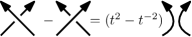
Figure 8. Alexander-Conway skein relation in the variable $(t^{\frac{1}{2}})^{4}$

Lemma 5.17.

The action of $\delta_{Z}$ is zero on the 4-dimensional direct summands of $Z\otimes Z$.

Proof.

We first consider the $Z=X({\smash{\text{\boldmath{$t$}}}})$ case for ${\smash{\text{\boldmath{$t$}}}}\in\mathcal{R}_{2}$. There is a surjection from $V({\smash{\text{\boldmath{$t$}}}})\otimes V({\smash{\text{\boldmath{$t$}}}})$ to $Z\otimes Z$ determined by the quotient $V({\smash{\text{\boldmath{$t$}}}})\twoheadrightarrow Z$ in each tensor factor. Although $V({\smash{\text{\boldmath{$t$}}}})\otimes V({\smash{\text{\boldmath{$t$}}}})$ does not decompose as a sum of irreducibles, Corollary 4.12 can still be applied to compute $R_{{\smash{\text{\boldmath{$t$}}}}}$ acting on specific vectors in $V({\smash{\text{\boldmath{$t$}}}})\otimes V({\smash{\text{\boldmath{$t$}}}})$ for generic $t$, which then descend to vectors in $Z\otimes Z$ after specializing parameters. That is, $R_{{\smash{\text{\boldmath{$t$}}}}}$ acts on $v_{0}\otimes v_{0}$ and $\Delta(E_{1}E_{2}E_{1}).(F_{1}F_{2}F_{1}v_{0}\otimes F_{1}F_{2}F_{1}v_{0})$ by $t_{1}^{2}t_{2}^{2}$ and $-t_{1}^{-2}$, respectively. Setting ${\smash{\text{\boldmath{$t$}}}}=(t,\pm 1)$ and taking the above quotient $V({\smash{\text{\boldmath{$t$}}}})\otimes V({\smash{\text{\boldmath{$t$}}}})\twoheadrightarrow Z\otimes Z$, these vectors are mapped to the highest weight vectors of the 4-dimensional summands of $Z\otimes Z$ indicated in Theorem 1.3. Then $R_{Z}-R^{-1}_{Z}$ acts by $t^{2}-t^{-2}$ on both of $x_{0}\otimes x_{0}$ and $\Delta(E_{1}E_{2}E_{1}).(F_{1}F_{2}F_{1}x_{0}\otimes F_{1}F_{2}F_{1}x_{0})$. Thus, $\delta_{Z}$ is zero on the corresponding 4-dimensional summands.

The $Z=Y({\smash{\text{\boldmath{$t$}}}})$ case for ${\smash{\text{\boldmath{$t$}}}}\in\mathcal{R}_{1}$ is identical, except the indices 1 and 2 are switched. For $Z=W(\zeta t,\pm t^{-1})$, we take the vectors $\Delta(E_{1})(F_{1}v_{0}\otimes F_{1}v_{0})$ and $\Delta(E_{2})(F_{2}v_{0}\otimes F_{2}v_{0})$. Generically, $R_{{\smash{\text{\boldmath{$t$}}}}}$ acts by $-t_{2}^{2}$ and $-t_{1}^{2}$, respectively. Therefore, $R_{Z}$ acts by $-t^{-2}$ and $-(\zeta t)^{2}=t^{2}$ on the corresponding summands of $Z\otimes Z$ whose highest weight vectors are $\Delta(E_{1})(F_{1}w_{0}\otimes F_{1}w_{0})$ and $\Delta(E_{2})(F_{2}w_{0}\otimes F_{2}w_{0})$. This shows that $\delta_{Z}$ acts as zero on these summands. ∎

Remark 5.18.

We consider $Z\in\{X(t,\pm 1),Y(\pm 1,t),W(\zeta t,\pm t^{-1})\}$ in our computations, and exclude $Z^{\prime}$ of the form $W(t,\pm\zeta t^{-1})$ because $\delta_{Z^{\prime}}=-2(t^{2}-t^{-2})$ on the 4-dimensional summands of $Z^{\prime}\otimes Z^{\prime}$. Replacing $R$ with $R^{-1}$ in $\delta_{Z^{\prime}}$ resolves this discrepancy. Since we recover the Alexander polynomial from these representations, which does not distinguish mirror images, using either convention is consistent with Theorem 1.3.

One can show that $\delta_{Z}$ acts by $-(t^{2}-t^{-2})$ on the 8-dimensional summand of $Z\otimes Z$.

Lemma 5.19.

Let $i_{U}$ and $\pi_{U}$ denote normalized inclusion and projection maps of the 8-dimensional summand $U$ into and out of $Z\otimes Z$. The trace of $\pi_{U}\circ(id_{Z}\otimes h_{Z})\circ i_{U}$ is zero.

Proof.

Since $1\otimes K_{2\rho}^{-1}\notin\Delta(\overline{U})$, $id_{Z}\otimes h_{Z}$ does not respect the decomposition of $Z\otimes Z$. To compute the trace of $\pi_{U}\circ(id_{Z}\otimes h_{Z})\circ i_{U}$, we must give a full description of $(id_{Z}\otimes h_{Z})\circ i_{U}$ with vectors in $Z\otimes Z$. We express the image of $(id_{Z}\otimes h_{Z})\circ i_{U}$ in terms of the direct sum basis from Theorem 1.3 in order to evaluate the projection $\pi_{U}$. Our presentation is such that the first term belongs to $U$ and the other terms belong to other summands i.e. $\pi_{U}$ is the restriction to the first term. For $Z=X(t,1)$, $(id_{Z}\otimes h_{Z})\circ i_{U}$ is the linear map

$$\Delta(E_{1}).(F_{1}x_{0}\otimes F_{1}x_{0})\mapsto \frac{-\zeta\left\lfloor t\right\rfloor}{t^{2}\left\lfloor\zeta t\right\rfloor}\Delta(E_{1}).(F_{1}x_{0}\otimes F_{1}x_{0})+\frac{\left\lfloor t\right\rfloor}{t\left\lfloor\zeta t\right\rfloor}\Delta(F_{1}).(x_{0}\otimes x_{0})$$

$$\Delta(F_{1}E_{1}).(F_{1}x_{0}\otimes F_{1}x_{0})\mapsto \frac{-1}{t^{2}}\Delta(F_{1}E_{1}).(F_{1}x_{0}\otimes F_{1}x_{0})$$

$$\Delta(F_{2}E_{1}).(F_{1}x_{0}\otimes F_{1}x_{0})\mapsto \frac{1}{t^{2}}\Delta(F_{2}E_{1}).(F_{1}x_{0}\otimes F_{1}x_{0})$$

$$\Delta(F_{1}F_{2}E_{1}).(F_{1}x_{0}\otimes F_{1}x_{0})\mapsto \frac{\zeta\left\lfloor t\right\rfloor}{t^{2}\left\lfloor\zeta t\right\rfloor}\Delta(F_{1}F_{2}E_{1}).(F_{1}x_{0}\otimes F_{1}x_{0})$$

$$+\frac{\left\lfloor t\right\rfloor}{t\left\lfloor\zeta t\right\rfloor\left\lfloor\zeta t^{2}\right\rfloor}\Delta(F_{1}F_{2}F_{1}).(x_{0}\otimes x_{0})$$

$$+\frac{2\zeta\left\lfloor t\right\rfloor}{t^{3}\left\lfloor\zeta t\right\rfloor\left\lfloor\zeta t^{2}\right\rfloor}\Delta(E_{1}E_{2}E_{1}).(F_{1}F_{2}F_{1}x_{0}\otimes F_{1}F_{2}F_{1}x_{0})$$

$$\Delta(F_{2}F_{1}E_{1}).(F_{1}x_{0}\otimes F_{1}x_{0})\mapsto \left(\frac{\zeta\left\lfloor\zeta t\right\rfloor}{t^{2}\left\lfloor t\right\rfloor}\Delta(F_{2}F_{1}E_{1})-\frac{2\zeta\left\lfloor t\right\rfloor}{t^{2}\left\lfloor\zeta t\right\rfloor}\Delta(F_{1}F_{2}E_{1})\right).(F_{1}x_{0}\otimes F_{1}x_{0})$$

$$-\frac{2\left\lfloor t\right\rfloor^{2}}{t\left\lfloor\zeta t^{2}\right\rfloor}\Delta(F_{1}F_{2}F_{1}).(x_{0}\otimes x_{0})$$

$$-\frac{2\zeta}{t^{2}}\Delta(E_{1}E_{2}E_{1}).(F_{1}F_{2}F_{1}x_{0}\otimes F_{1}F_{2}F_{1}x_{0})$$

$$\Delta(F_{1}F_{2}F_{1}E_{1}).(F_{1}x_{0}\otimes F_{1}x_{0})\mapsto \frac{-1}{t^{2}}\Delta(F_{1}F_{2}F_{1}E_{1}).(F_{1}x_{0}\otimes F_{1}x_{0})$$

$$\Delta(F_{2}F_{1}F_{2}E_{1}).(F_{1}x_{0}\otimes F_{1}x_{0})\mapsto \frac{1}{t^{2}}\Delta(F_{2}F_{1}F_{2}E_{1}).(F_{1}x_{0}\otimes F_{1}x_{0})$$

$$\Delta(F_{1}F_{2}F_{1}F_{2}E_{1}).(F_{1}x_{0}\otimes F_{1}x_{0})\mapsto -\frac{\zeta\left\lfloor\zeta t\right\rfloor}{t^{2}\left\lfloor t\right\rfloor}\Delta(F_{1}F_{2}F_{1}F_{2}E_{1}).(F_{1}x_{0}\otimes F_{1}x_{0})$$

$$+\frac{2\zeta}{\left\lfloor\zeta t^{2}\right\rfloor t^{3}}\Delta(F_{2}F_{1}E_{1}E_{2}E_{1})(F_{1}F_{2}F_{1}x_{0}\otimes F_{1}F_{2}F_{1}x_{0}).$$

Composing with the projection to $U$, we see that $\pi_{U}\circ(id_{Z}\otimes h_{Z})\circ i_{U}$ is traceless.

The cases $Z\in\{X(t,-1),Y(\pm 1,t)\}$ are similar. The action on $U=V(-t^{2},t^{-2})$ in the $Z=W(it,t^{-1})$ case is given from the mapping below, and the claim follows.

$$w_{0}\otimes w_{0}\mapsto -w_{0}\otimes w_{0}$$

$$\Delta(F_{1}).(w_{0}\otimes w_{0})\mapsto \frac{\zeta\left\lfloor\zeta t\right\rfloor}{\left\lfloor t\right\rfloor}\Delta(F_{1}).(w_{0}\otimes w_{0})+\frac{2\zeta}{\left\lfloor t^{2}\right\rfloor}\Delta(E_{1}).(F_{1}w_{0}\otimes F_{1}w_{0})$$

$$\Delta(F_{2}).(w_{0}\otimes w_{0})\mapsto \frac{\zeta\left\lfloor t\right\rfloor}{\left\lfloor\zeta t\right\rfloor}\Delta(F_{2}).(w_{0}\otimes w_{0})+\frac{2t}{\left\lfloor t^{2}\right\rfloor}\Delta(E_{2}).(F_{2}w_{0}\otimes F_{2}w_{0})$$

$$\Delta(F_{1}F_{2}).(w_{0}\otimes w_{0})\mapsto \Delta(F_{1}F_{2}).(w_{0}\otimes w_{0})-\frac{2\left\lfloor t\right\rfloor}{t\left\lfloor\zeta t\right\rfloor\left\lfloor\zeta t^{2}\right\rfloor}\Delta(F_{2}E_{1}).(F_{1}w_{0}\otimes F_{1}w_{0})$$

$$+\frac{2\zeta t}{\left\lfloor\zeta t^{2}\right\rfloor}\Delta(F_{2}E_{2}).(F_{2}w_{0}\otimes F_{2}w_{0})$$

$$\Delta(F_{2}F_{1}).(w_{0}\otimes w_{0})\mapsto \Delta(F_{2}F_{1}).(w_{0}\otimes w_{0})-\frac{2\zeta t\left\lfloor\zeta t\right\rfloor}{\left\lfloor t\right\rfloor\left\lfloor\zeta t^{2}\right\rfloor}\Delta(F_{2}E_{2}).(F_{2}w_{0}\otimes F_{2}w_{0})$$

$$+\frac{2}{t\left\lfloor\zeta t^{2}\right\rfloor}\Delta(F_{2}E_{1}).(F_{1}w_{0}\otimes F_{1}w_{0})$$

$$\Delta(F_{1}F_{2}F_{1}).(w_{0}\otimes w_{0})\mapsto -\frac{\zeta\left\lfloor\zeta t\right\rfloor}{\left\lfloor t\right\rfloor}\Delta(F_{1}F_{2}F_{1}).(w_{0}\otimes w_{0})-\frac{4\zeta}{t\left\lfloor t^{4}\right\rfloor}\Delta(F_{1}F_{2}E_{1}).(F_{1}w_{0}\otimes F_{1}w_{0})$$

$$\Delta(F_{2}F_{1}F_{2}).(w_{0}\otimes w_{0})\mapsto -\frac{\zeta\left\lfloor t\right\rfloor}{\left\lfloor\zeta t\right\rfloor}\Delta(F_{2}F_{1}F_{2}).(w_{0}\otimes w_{0})-\frac{t}{2\left\lfloor t\right\rfloor^{2}\left\lfloor\zeta t\right\rfloor^{2}}\Delta(F_{1}F_{2}E_{2}).(F_{2}w_{0}\otimes F_{2}w_{0})$$

$$\Delta(F_{1}F_{2}F_{1}F_{2}).(w_{0}\otimes w_{0})\mapsto -\Delta(F_{1}F_{2}F_{1}F_{2}).(w_{0}\otimes w_{0})\qed$$

Proof.

Fix a four-dimensional representation $Z$ to be any of $X({\smash{\text{\boldmath{$t$}}}})$, $Y({\smash{\text{\boldmath{$t$}}}})$, or $W({\smash{\text{\boldmath{$t$}}}})$, and assume $t$ is chosen so that $Z$ is well-defined and irreducible. Moreover, we may assume a specific form $Z\in\{X(t,\pm 1),Y(\pm 1,t),W(\zeta t,\pm t^{-1})\}$ for some generic $t$, as explained in Remark 5.18. The Alexander-Conway relation is encoded by $\delta_{Z}$ and is zero on both 4-dimensional summands of $Z\otimes Z$ by Lemma 5.17. We next compute the quantum invariant for the closure of any intertwiner $A\in\operatorname{End}_{\overline{U}^{H}}(Z\otimes Z)$ with the skein relation $\delta_{Z}$ applied to it. In particular, we show that the closure of any (2,2)-tangle is compatible with the skein relation.

By Theorem 1.3, $Z\otimes Z$ is semisimple and multiplicity free. Therefore, $\delta_{Z}A$ acts by scalars on each summand and Lemma 5.17 states that only the action on the 8-dimensional summand $U$ may be nonzero. We denote this scalar by $\widehat{\delta_{Z}A}_{U}$. The trace of $(id_{Z}\otimes h_{Z})\delta_{Z}A$ is computed in Figure 9, the dot indicates the application of $h_{Z}$. In the first equality, we sum over all summands of $Z\otimes Z$, with the forks indicating projection and inclusion. All terms in the sum are zero except the one which factors through $U$, on which, ${\delta_{Z}}{A}$ acts by $\widehat{\delta_{Z}A}_{U}$. The diagram that remains is equal to the trace of $\pi_{U}\circ(id\otimes h_{Z})\circ i_{U}$, and by Lemma 5.19 this is zero.

Figure 9. Proof of Theorem 1.3

∎

We expect that our result extends to the multi-colored case, where all components are colored by the same family of representations.

6. Properties of $\Delta_{\mathfrak{sl}_{3}}$

In this section, we prove several properties of $\Delta_{\mathfrak{sl}_{3}}$. In Corollary 6.2 we show that certain automorphisms of $\mathfrak{sl}_{3}$ determine symmetries of $\Delta_{\mathfrak{sl}_{3}}$. We prove in Lemma 6.3 that $\Delta_{\mathfrak{g}}$ is preserved under the map ${\smash{\text{\boldmath{$t$}}}}\mapsto{\smash{\text{\boldmath{$-t^{-1}$}}}}$, assuming $\overline{U}^{H}$ is standard pre-triangular. We then discuss the skein relation for $\Delta_{\mathfrak{sl}_{3}}$, which we obtain from the characteristic polynomial of the $R_{{\smash{\text{\boldmath{$t$}}}}}$. We also discuss a method to compute the invariant on torus knots and give the formula for ${(2n+1,2)}$ torus knots explicitly. We end this section by proving Theorem 1.1, that $\Delta_{\mathfrak{sl}_{3}}$ dominates the Alexander polynomial for knots. More precisely, evaluating $\Delta_{\mathfrak{sl}_{3}}(K)$ at $t_{2}=\pm 1$ or $t_{2}=\pm it_{1}^{-1}$ yields the Alexander polynomial in the variable $t_{1}^{4}$ for any knot $K$.

Lemma 6.1.

Let $\tau$ an automorphism of the Dynkin diagram of $\mathfrak{sl}_{3}$. Then $\tau$ determines an automorphism of $\overline{U}^{H}_{\zeta}(\mathfrak{sl}_{3})\operatorname{-wmod}$ as a ribbon category.

Proof.

Define $\widehat{\tau}$ to be an algebra automorphism of $\overline{U}^{H}_{\zeta}$ so that $\widehat{\tau}(X_{i})=X_{\tau(i)}$ for $X\in\{E,F,K,H\}$. Each of its Hopf algebra maps is intertwined by $\widehat{\tau_{h}}$. We check that $\check{R}$ is invariant under $\widehat{\tau_{h}}\otimes\widehat{\tau_{h}}$ in the $\mathfrak{sl}_{3}$ case explicitly. Recall

$$\check{R}= (1\otimes 1+(\zeta-\zeta^{-1})E_{1}\otimes F_{1})(1\otimes 1+(\zeta-\zeta^{-1})E_{12}\otimes F_{12})(1\otimes 1+(\zeta-\zeta^{-1})E_{2}\otimes F_{2})$$

$$= 1\otimes 1+2\zeta(E_{1}\otimes F_{1}+E_{2}\otimes F_{2})+(2\zeta E_{12}\otimes F_{12}-4E_{1}E_{2}\otimes F_{1}F_{2})$$

$$-4(E_{1}E_{12}\otimes F_{1}F_{12}+E_{12}E_{2}\otimes F_{12}F_{2})-8\zeta(E_{1}E_{12}E_{2}\otimes F_{1}F_{12}F_{2})$$

$$= 1\otimes 1+2\zeta(E_{1}\otimes F_{1}+E_{2}\otimes F_{2})+2\zeta(E_{1}E_{2}\otimes F_{2}F_{1}+E_{2}E_{2}\otimes F_{1}F_{2})$$

$$-2(E_{1}E_{2}\otimes F_{1}F_{2}+E_{2}E_{1}\otimes F_{2}F_{1})-4\zeta(E_{1}E_{2}E_{1}\otimes F_{1}F_{2}F_{1}+E_{2}E_{1}E_{2}\otimes F_{2}F_{1}F_{2})$$

$$+8(E_{1}E_{2}E_{1}E_{2}\otimes F_{1}F_{2}F_{1}F_{2})$$

and that $E_{1}E_{2}E_{1}E_{2}=E_{2}E_{1}E_{2}E_{1}$, $F_{1}F_{2}F_{1}F_{2}=F_{2}F_{1}F_{2}F_{1}$ since $E_{12}^{2}=F_{12}^{2}=0$. We see that this expression is preserved by $\widehat{\tau}\otimes\widehat{\tau}$. Thus, $\widehat{\tau}\otimes\widehat{\tau}(\check{R})=\check{R}$.

Let $\widetilde{\tau}:\overline{U}^{H}_{\zeta}\text{-wmod}\to\overline{U}^{H}_{\zeta}\operatorname{-wmod}$ be the functor defined by $\widetilde{\tau}\left((V,\rho)\right)=(V,\rho\circ\widehat{\tau})$ on representations and is the identity on morphisms as linear maps. That is, if $\mathsf{F}:\overline{U}^{H}_{\zeta}\text{-wmod}\to\text{Vect}$ is the forgetful functor, then $\mathsf{F}\circ\widetilde{\tau}=\mathsf{F}$. Since $\widehat{\tau}$ is a Hopf algebra morphism, $\widetilde{\tau}$ is canonically a strict $\otimes$-functor and $\widetilde{\tau}(V^{*})=\widetilde{\tau}(V)^{*}$ up to canonical isomorphism. Therefore, $\widetilde{\tau}(ev_{V})=ev_{\widetilde{\tau}(V)}$ up to canonical isomorphism and similarly for the other duality maps.

We prove $\widetilde{\tau}(\textit{{c}}_{V,W})=\textit{{c}}_{\widetilde{\tau}(V),\widetilde{\tau}(W)}$ for any weight representations $(V,\rho)$ and $(W,\rho^{\prime})$, noting that $\rho$ and $\rho^{\prime}$ are suppressed in our notation for the braiding. Since $\mathsf{F}$ is injective on morphisms, it is enough to show that $\mathsf{F}(\widetilde{\tau}(\textit{{c}}_{V,W}))=\mathsf{F}(\textit{{c}}_{\widetilde{\tau}(V),\widetilde{\tau}(W)})$, which is the same as showing $\mathsf{F}(\textit{{c}}_{V,W})=\mathsf{F}(\textit{{c}}_{\widetilde{\tau}(V),\widetilde{\tau}(W)})$. For this proof and its corollary, we distinguish the braiding $\textit{{c}}_{V,W}$ as an abstract morphism in $\overline{U}^{H}\operatorname{-wmod}$ from the linear map realizing it. To be more precise, the realization given in (64) is, in fact, $\mathsf{F}(\textit{{c}}_{V,W})$. Since $\widehat{\tau}\otimes\widehat{\tau}(\check{R})=\check{R}$, we have:

$$\mathsf{F}(\textit{{c}}_{\widetilde{\tau}(V),\widetilde{\tau}(W)}) =P\circ E_{\rho\circ\widehat{\tau},\rho^{\prime}\circ\widehat{\tau}}\circ(\rho\circ\widehat{\tau}\otimes\rho^{\prime}\circ\widehat{\tau})(\check{R})=P\circ E_{\rho\circ\widehat{\tau},\rho^{\prime}\circ\widehat{\tau}}\circ(\rho\otimes\rho^{\prime})(\check{R}).$$ (80)

Suppose that $\rho(H_{i})v=\mu_{i}v$ and $\rho^{\prime}(H_{i})w=\nu_{i}w$, then $\rho\circ\widehat{\tau}(H_{i})v=\rho(H_{\tau(i)})v=\mu_{\tau(i)}v$ and similarly $\rho^{\prime}\circ\widetilde{\tau}(H_{i})w=\nu_{\tau(i)}w$. Therefore,

$$E_{\rho\circ\widehat{\tau},\rho^{\prime}\circ\widehat{\tau}}(v\otimes w) =\zeta^{{\sum_{ij}d_{i}(A^{-1})_{ij}\mu_{\tau(i)}\nu_{\tau(j)}}}(v\otimes w)$$

$$=\zeta^{{\sum_{ij}d_{i}(A^{-1})_{\tau^{-1}(i)\tau^{-1}(j)}\mu_{i}\nu_{j}}}(v\otimes w)=E_{\rho,\rho^{\prime}}(v\otimes w)$$

by invariance of the Cartan matrix under $\tau$. Continuing from (80),

$$\mathsf{F}(\textit{{c}}_{\widetilde{\tau}(V),\widetilde{\tau}(W)})=P\circ E_{\rho\circ\widehat{\tau},\rho^{\prime}\circ\widehat{\tau}}\circ(\rho\otimes\rho^{\prime})(\check{R})=\mathsf{F}(\textit{{c}}_{V,W}).$$

Thus, $\widetilde{\tau}(\textit{{c}}_{V,W})=\textit{{c}}_{\widetilde{\tau}(V),\widetilde{\tau}(W)}$.

In Proposition 5.3, we expressed the ribbon structure of $\overline{U}^{H}_{\zeta}\operatorname{-wmod}$ in terms of the braiding and pivotal action by $\operatorname{tr}_{R}(\textit{{c}}_{V,V})=\theta_{V}$. Therefore, $\widetilde{\tau}(\theta_{{V}})=\theta_{\widetilde{\tau}(V)}$ and $\widetilde{\tau}$ is an automorphism of $\overline{U}^{H}_{\zeta}\operatorname{-wmod}$ as a ribbon category. ∎

Corollary 6.2.

Let $\tau$ be an automorphism of the Dynkin diagram of $\mathfrak{sl}_{3}$. For any link $L$, $\tau$ determines a symmetry of the polynomial invariant:

$$\Delta_{\mathfrak{sl}_{3}}(L)(t_{1},t_{2})=\Delta_{\mathfrak{sl}_{3}}(L)(t_{\tau(1)},t_{\tau(2)}).$$ (81)

Proof.

As above, $\widetilde{\tau}$ is the automorphism of $\overline{U}^{H}\operatorname{-wmod}$ as a ribbon category given by precomposing with $\widehat{\tau}$. Moreover, $\tau$ induces a functor $\widetilde{\tau}^{\prime}$ on $\overline{U}\operatorname{-wmod}$ which is intertwined with $\widetilde{\tau}$ by the functor that forgets the actions of $H_{1},H_{2}$. Let $\tau t$ denote $(t_{\tau(1)},t_{\tau(2)})$. If $v_{0}$ is the highest weight vector in $V({\smash{\text{\boldmath{$t$}}}})$, then $\rho\circ\widehat{\tau}^{\prime}(K_{i})v_{0}=\rho(K_{\tau(i)})v_{0}=t_{\tau(i)}v_{0}$. Thus, $\widetilde{\tau}^{\prime}(V({\smash{\text{\boldmath{$t$}}}}))=V({\smash{\text{\boldmath{$\tau t$}}}})$.

Let $\langle T\rangle_{V({\smash{\text{\boldmath{$t$}}}})}$ denote the action of a (1,1)-tangle representative of a zero-sum framed link $L$ as an endomorphism of an irreducible representation $(V({\smash{\text{\boldmath{$t$}}}}),\rho)$. Since $\langle T\rangle_{V({\smash{\text{\boldmath{$t$}}}})}$ is given by a composition of normalized braidings, evaluations, and co-evaluations, Lemma 6.1 implies $\widetilde{\tau}^{\prime}(\langle T\rangle_{V({\smash{\text{\boldmath{$t$}}}})})=\langle T\rangle_{\widetilde{\tau}^{\prime}(V({\smash{\text{\boldmath{$t$}}}}))}=\langle T\rangle_{V({\smash{\text{\boldmath{$\tau t$}}}})}$. Applying the forgetful functor $\mathsf{F}$, we have the equality of linear maps $\mathsf{F}(\langle T\rangle_{V({\smash{\text{\boldmath{$t$}}}})})=\mathsf{F}(\widetilde{\tau}^{\prime}(\langle T\rangle_{V({\smash{\text{\boldmath{$t$}}}})}))=\mathsf{F}(\langle T\rangle_{V({\smash{\text{\boldmath{$\tau t$}}}})})$. Since $\mathsf{F}(\langle T\rangle_{V({\smash{\text{\boldmath{$t$}}}})})$ is equal to $\Delta_{\mathfrak{sl}_{3}}(L)(t_{1},t_{2})$ times the identity, the equality in (81) holds. ∎

Lemma 6.3.

Suppose $\overline{U}^{H}$ is standard pre-triangular. Let $L$ be an oriented link and $-L$ the same link with all orientations reversed. Then

$$\Delta_{\mathfrak{g}}(-L)(t_{1},\dots,t_{n})=\Delta_{\mathfrak{g}}(L)(-t_{1}^{-1},\dots,-t_{n}^{-1}).$$ (82)

Proof.

Recall from Proposition 3.3 that $V({\smash{\text{\boldmath{$t$}}}})^{*}\cong V({\smash{\text{\boldmath{$-t^{-1}$}}}})$, and by Theorem 5.11 both $V({\smash{\text{\boldmath{$t$}}}})$ and its dual are ambidextrous for generic $t$. Since the morphism assigned to the open Hopf link colored by $V({\smash{\text{\boldmath{$t$}}}})$ and $V({\smash{\text{\boldmath{$t$}}}})^{*}$ is nonzero, we may apply [GPT09, Proposition 19]. Thus, reversing the orientation of a component of $L$ is equivalent to coloring it by $V({\smash{\text{\boldmath{$t$}}}})^{*}$. Therefore, $\Delta_{\mathfrak{g}}(-L)$ is computed from coloring all components of $L$ by $V({\smash{\text{\boldmath{$-t^{-1}$}}}})$. ∎

In all known examples, we have found that $\Delta_{\mathfrak{sl}_{3}}(L)(t_{1},t_{2})=\Delta_{\mathfrak{sl}_{3}}(L)(-t_{1}^{-1},-t_{2}^{-1})$. In particular, this equality holds for the non-invertible knots $\mathsf{8_{17}}$, $\mathsf{9_{32}}$, and $\mathsf{9_{33}}$.

Applying these symmetries of the unrolled $\mathfrak{sl}_{3}$ invariant, we find that the polynomial contains redundant information. In Section 7, our presentation of the knot invariants accounts for these symmetries.

Lemma 6.4.

Suppose that ${\smash{\text{\boldmath{$t$}}}}\in\mathcal{R}$ so that $V({\smash{\text{\boldmath{$t$}}}})$ belongs to the exact sequence

$$0\rightarrow V_{1}\to V({\smash{\text{\boldmath{$t$}}}})\rightarrow V_{2}\rightarrow 0,$$ (83)

where $V_{1}$ and $V_{2}$ are ambidextrous. Then for any knot $K$, $\Delta_{V({\smash{\text{\boldmath{$t$}}}})}(K)=\Delta_{V_{1}}(K)=\Delta_{V_{2}}(K)$.

Proof.

Given that $V_{1}$ and $V_{2}$ are ambidextrous, $\Delta_{V_{1}}$ and $\Delta_{V_{2}}$ are well-defined. By Remark 5.12, $\Delta_{V({\smash{\text{\boldmath{$t$}}}})}$ is also well-defined. Let $b\in B_{n}$ be a braid representative for a knot $K$, and $T$ the (1,1)-tangle obtained from closing the $n-1$ right strands of $\overline{z}(b)$, with $\overline{z}$ as in Figure 7. Recall that $b$ acts on $V({\smash{\text{\boldmath{$t$}}}})^{\otimes n}$ via the representation $\overline{\psi_{n}}$ given following Remark 5.13. For generic $t$, $\langle T\rangle_{V({\smash{\text{\boldmath{$t$}}}})}=\operatorname{tr}_{R}^{n-1}(\overline{\psi_{n}}(b))$ acts on $V({\smash{\text{\boldmath{$t$}}}})$ by the scalar $\Delta_{V({\smash{\text{\boldmath{$t$}}}})}(K)$. Upon specializing $t$ so that $V({\smash{\text{\boldmath{$t$}}}})$ is reducible, $\langle T\rangle_{V({\smash{\text{\boldmath{$t$}}}})}$ still acts by a multiple of the identity. By naturality of the braiding and pivotal structure discussed in Section 4, the inclusion $i:V_{1}\hookrightarrow V({\smash{\text{\boldmath{$t$}}}})$ satisfies the intertwiner relation

$$\Delta_{V({\smash{\text{\boldmath{$t$}}}})}(K)\cdot i=\langle T\rangle_{V({\smash{\text{\boldmath{$t$}}}})}\circ i=i\circ\langle T\rangle_{V_{1}}=\Delta_{V_{1}}(K)\cdot i.$$

Therefore, $\Delta_{V_{1}}(K)=\Delta_{V({\smash{\text{\boldmath{$t$}}}})}(K)$.

Similarly, the surjection $V({\smash{\text{\boldmath{$t$}}}})\twoheadrightarrow V_{2}$ intertwines the scalar action. This implies that $\langle T\rangle_{V_{2}}$ acts on $V_{2}$ by $\Delta_{V_{2}}(K)=\Delta_{V({\smash{\text{\boldmath{$t$}}}})}(K)$. ∎

Proof.

The first claim is an immediate consequence of Theorem 1.3 and Lemma 6.4. The second claim follows from checking which evaluations of $\Delta_{\mathfrak{sl}_{3}}$ simultaneously yield the Alexander polynomial for the knots $\mathsf{3_{1}}$ and $\mathsf{4_{1}}$. ∎

Remark 6.5.

Lemma 6.4 only applies to knots. If a link were colored by reducible representations $V({\smash{\text{\boldmath{$t$}}}})$, only the color of the open strand could be replaced by $V_{1}$ or $V_{2}$. All other strands in the diagram remain colored by $V({\smash{\text{\boldmath{$t$}}}})$.

The following is a corollary of the above symmetries and Theorem 1.1.

Corollary 6.6.

Suppose that for some link $L$, $\Delta_{\mathfrak{sl}_{3}}(L)=\Delta_{\mathfrak{sl}_{3}}(-L)$. Then $\Delta_{\mathfrak{sl}_{3}}(L)(t_{1},t_{2})$ is a Laurent polynomial in $t_{1}^{2}$ and $t_{2}^{2}$.

Proof.

By the properties given in Corollary 6.2 and our assumption, $\Delta_{\mathfrak{sl}_{3}}(L)(t_{1},t_{2})$ is a linear combination Laurent polynomials which are symmetric under $t_{1}^{i}t_{2}^{j}\mapsto(-1)^{i+j}t_{1}^{-i}t_{2}^{-j}$ and $t_{1}^{i}t_{2}^{j}\mapsto t_{1}^{j}t_{2}^{i}$. If $\Delta_{\mathfrak{sl}_{3}}(L)(t_{1},t_{2})$ is a polynomial whose degree in $t_{1}$ is $n$, then for some integers $c,a_{i},b_{i}$, and $c_{kl}$ we have:

$$\Delta_{\mathfrak{sl}_{3}}(t_{1},t_{2})=c +\sum_{i=1}^{n}\left[a_{i}(t_{1}^{i}t_{2}^{i}+t_{1}^{-i}t_{2}^{-i})+b_{i}(t_{1}^{i}t_{2}^{-i}+t_{1}^{-i}t_{2}^{i})\right]$$

$$+\sum_{\begin{subarray}{c}k=1\\ |l|<k\end{subarray}}^{n}c_{kl}\left[t_{1}^{k}t_{2}^{l}+(-1)^{k+l}t_{1}^{-k}t_{2}^{-l}+t_{1}^{l}t_{2}^{k}+(-1)^{k+l}t_{1}^{-l}t_{2}^{-k}\right].$$

By Theorem 1.1, $\Delta_{\mathfrak{sl}_{3}}(t,\zeta t^{-1})=\Delta_{\mathfrak{sl}_{3}}(t,-\zeta t^{-1})$. And so,

$$\sum_{i=1}^{n}\left[a_{i}(\zeta^{i}+\zeta^{-i})+b_{i}(\zeta^{-i}t^{2i}+\zeta^{i}t^{-2i})\right]+\sum_{\begin{subarray}{c}k=1\\ |l|<k\end{subarray}}^{n}c_{kl}\left[t^{k-l}(\zeta^{l}+(-1)^{k+l}\zeta^{-k})+t^{l-k}((-1)^{k+l}\zeta^{-l}+\zeta^{k})\right]$$

$$= \sum_{i=1}^{n}\left[a_{i}(\zeta^{-i}+\zeta^{i})+b_{i}(\zeta^{i}t^{2i}+\zeta^{-i}t^{-2i})\right]+\sum_{\begin{subarray}{c}k=1\\ |l|<k\end{subarray}}^{n}c_{kl}\left[t^{k-l}(\zeta^{-l}+(-1)^{k+l}\zeta^{k})+t^{l-k}((-1)^{k+l}\zeta^{l}+\zeta^{-k})\right].$$

Comparing terms of degree $k-l$,

$$c_{kl}t^{k-l}(\zeta^{l}+(-1)^{k+l}\zeta^{-k}) =c_{kl}t^{k-l}(\zeta^{-l}+(-1)^{k+l}\zeta^{k})$$

$$c_{kl}(\zeta^{l}-\zeta^{-l}) =c_{kl}(\zeta^{k}-\zeta^{-k})(-1)^{k+l}.$$

This implies that $c_{kl}=0$ whenever $k$ and $l$ have different parity.

We now consider the evaluations of $\Delta_{\mathfrak{sl}_{3}}$ at $(t,1)$ and $(t,-1)$. Only accounting for terms where $k$ and $l$ have the same parity, we have

$$\sum_{i=1}^{n}\left[a_{i}(t^{i}+t^{-i})+b_{i}(t^{i}+t^{-i})\right]+\sum_{\begin{subarray}{c}k=1\\ |l|<k\end{subarray}}^{n}c_{kl}\left[t^{k}+t^{-k}+t^{l}+t^{-l}\right]$$

equals

$$\sum_{i=1}^{n}\left[a_{i}(-1)^{i}(t^{i}+t^{-i})+(-1)^{i}b_{i}(t^{i}+t^{-i})\right]+\sum_{\begin{subarray}{c}k=1\\ |l|<k\end{subarray}}^{n}c_{kl}(-1)^{k}\left[t^{k}+t^{-k}+t^{l}+t^{-l}\right].$$

Comparing each term, we see that each coefficient of odd index vanishes. ∎

6.1. Properties Derived from Powers of $R_{{\smash{\text{\boldmath{$t$}}}}}$

The skein relation and value of $\Delta_{\mathfrak{sl}_{3}}$ on two strand torus knots are both derived from the characteristic (minimal) polynomial of $R_{{\smash{\text{\boldmath{$t$}}}}}$. The former is obtained from (84), and the latter is stated in Theorem 1.1.

Proposition 6.7.

There is a nine-term skein relation for $\Delta_{\mathfrak{sl}_{3}}$.

Proof.

Let $r$ be the $8\times 8$ matrix which appears in Corollary 4.12. By the Cayley-Hamilton Theorem, the characteristic polynomial of $r$ determines a relation among powers of itself. Therefore, the characteristic polynomial of $R_{{\smash{\text{\boldmath{$t$}}}}}$ is the characteristic polynomial of $r$ raised to the power $\dim V({\smash{\text{\boldmath{$t$}}}})$. Thus, $R_{{\smash{\text{\boldmath{$t$}}}}}$ is a solution to the equation given by $r$. This relation takes the form

$$(R_{{\smash{\text{\boldmath{$t$}}}}}^{2}+id)(t_{1}^{2}id+R_{{\smash{\text{\boldmath{$t$}}}}})(t_{1}^{2}R_{{\smash{\text{\boldmath{$t$}}}}}+id)(t_{2}^{2}id+R_{{\smash{\text{\boldmath{$t$}}}}})(t_{2}^{2}R_{{\smash{\text{\boldmath{$t$}}}}}+id)(t_{1}^{2}t_{2}^{2}id-R_{{\smash{\text{\boldmath{$t$}}}}})(t_{1}^{2}t_{2}^{2}R_{{\smash{\text{\boldmath{$t$}}}}}-id)=0.$$ (84)

After expansion and normalization, this implies the palindromic relation

$$c_{0}R_{{\smash{\text{\boldmath{$t$}}}}}^{0}+\sum_{i=1}^{4}c_{i}\left(R_{{\smash{\text{\boldmath{$t$}}}}}^{i}+R_{{\smash{\text{\boldmath{$t$}}}}}^{-i}\right)=0,$$

for some $c_{0},\dots,c_{4}\in\mathbb{Z}[t_{1}^{\pm 2},t_{2}^{\pm 2}]$ determined by (84). Replacing each factor of $R_{{\smash{\text{\boldmath{$t$}}}}}$ with a diagrammatic strand crossing and $R_{{\smash{\text{\boldmath{$t$}}}}}^{0}$ by two vertical strands, we obtain the skein relation. ∎

Similar to how we used the characteristic polynomial of the $R$-matrix to determine the skein relation, other characteristic polynomials yield relations among families of torus knots. Let $q$ be a prime number, and $r$ any positive integer less than $q$. Then for each $0<n<q$, we have that $qn+r$ and $q$ are coprime. Define

$$\beta_{q}=\left(\prod_{i=0}^{q-2}id^{\otimes i}\otimes R_{{\smash{\text{\boldmath{$t$}}}}}\otimes id^{\otimes q-i-2}\right),$$ (85)

which acts on $V({\smash{\text{\boldmath{$t$}}}})^{\otimes q}$. Then the characteristic polynomial of $\beta_{q}^{q}$ is some equation of the form

$$\sum_{i=0}^{8^{q}}a_{i}\beta_{q}^{qi}=0.$$ (86)

Multiplying this equation by $\beta_{q}^{r}$ implies that the invariants of the torus knots of types $(r,q),(q+r,q),\dots,((8^{q}-1)q+r,q)$ determine the invariant for the $(8^{q}q+r,q)$ torus knot. With this information and after multiplying equation (86) by $\beta_{q}^{r+1}$, we can deduce the invariant for the $((8^{q}+1)q+r,q)$ torus knot and so on. This implies a recursion relation for all torus knots $T_{nq+r,q}$, which can then be converted to an explicit function of $n$. The resulting expression for the $q=2,r=1$ case is stated as a theorem below.

Remark 6.8.

Observe that the expression for these torus knots breaks into three terms. One pair of terms exchange the roles of $t_{1}$ and $t_{2}$, while the other is symmetric in $t_{1}$ and $t_{2}$.

7. Values of $\Delta_{\mathfrak{sl}_{3}}$

In this section, we give the value of the unrolled restricted quantum $\mathfrak{sl}_{3}$ invariant for all prime knots with at most seven crossings, as well as some higher crossing knots. We have referred to [KA] for their list of prime knots and braid presentations. Among these examples are knots that compare $\Delta_{\mathfrak{sl}_{3}}$ to other well-known invariants. The HOMFLY polynomial does not distinguish the knot $\mathsf{11_{n34}}$ from $\mathsf{11_{n42}}$ nor does it distinguish $\mathsf{5_{1}}$ and $\mathsf{10_{132}}$, but $\Delta_{\mathfrak{sl}_{3}}$ does. The Jones polynomial differentiates $\mathsf{6_{1}}$ and $\mathsf{9_{46}}$, but $\Delta_{\mathfrak{sl}_{3}}$ does not. The Jones polynomial and the $\mathfrak{sl}_{3}$ invariant both distinguish $\mathsf{8_{9}}$ from $\mathsf{10_{155}}$; however, the Alexander polynomial does not.

As indicated by Question 1.3, $\Delta_{\mathfrak{sl}_{3}}(L)=\Delta_{\mathfrak{sl}_{3}}(-L)$ in all known examples. By the results of Section 6, it is enough to specify the coefficient of $t_{1}^{2a}t_{2}^{2b}$ in $\Delta_{\mathfrak{sl}_{3}}(L)$ for each $(a,b)$ in the cone

$$C=\{(a,b)\in\mathbb{Z}^{2}|a\geq 0\text{ and }|b|\leq a\}.$$ (87)

The coefficients of various knots can be found in Figures 10 and 11 below. We have boxed the leftmost value on each cone, it has coordinates $(0,0)$ and is the constant term in the polynomial invariant for the indicated knot. We do not label zeros outside of the convex hull of nonzero entries in the cone. From the values given, we can reconstruct $\Delta_{\mathfrak{sl}_{3}}$ since the coefficient in position $(a,b)$ is equal to those in positions $(b,a)$, $(-a,-b)$, and $(-b,-a)$. For example, the data for the trefoil knot $\mathsf{3_{1}}$ is given in Figure 10 and the associated Laurent polynomial is

$$\Delta_{\mathfrak{sl}_{3}}(\mathsf{3_{1}})(t_{1},t_{2})= (t_{1}^{4}t_{2}^{4}+t_{1}^{-4}t_{2}^{-4})-(t_{1}^{4}t_{2}^{2}+t_{1}^{2}t_{2}^{4}+t_{1}^{-4}t_{2}^{-2}+t_{1}^{-2}t_{2}^{-4})+(t_{1}^{4}+t_{2}^{4}+t_{1}^{-4}+t_{2}^{-4})$$

$$+2(t_{1}^{2}t_{2}^{2}+t_{1}^{-2}t_{2}^{-2})-2(t_{1}^{2}+t_{2}^{2}+t_{1}^{-2}+t_{2}^{-2})+(t_{1}^{2}t_{2}^{-2}+t_{1}^{-2}t_{2}^{2})+1.$$

(a) $\mathsf{3_{1}}$

(b) $\mathsf{4_{1}}$

(c) $\mathsf{5_{1}}$

(d) $\mathsf{5_{2}}$

(e) $\mathsf{6_{1}}$

(f) $\mathsf{6_{2}}$

(g) $\mathsf{6_{3}}$

(h) $\mathsf{7_{1}}$

(i) $\mathsf{7_{2}}$

(j) $\mathsf{7_{3}}$

(k) $\mathsf{7_{4}}$

(l) $\mathsf{7_{5}}$

(m) $\mathsf{7_{6}}$

(n) $\mathsf{7_{7}}$

Figure 10. The value of $\Delta_{\mathfrak{sl}_{3}}$ for all prime knots with fewer than seven crossings.

(a) $\mathsf{8_{9}}$

(b) $\mathsf{8_{17}}$

(c) $\mathsf{9_{32}}$

(d) $\mathsf{9_{33}}$

(e) $\mathsf{9_{46}}$

(f) $\mathsf{10_{132}}$

(g) $\mathsf{10_{155}}$

(h) $\mathsf{11_{n34}}$

(i) $\mathsf{11_{n42}}$

(j) $\text{Wh}^{0}(\mathsf{3_{1}})$

Figure 11. The value of $\Delta_{\mathfrak{sl}_{3}}$ for some prime knots with more than seven crossings.

The following properties are true in all computed examples, but they have not been proven.

Remark 7.1.

Using Theorem 1.1 and the symmetries of the invariant, we can recover the coefficients of Alexander polynomial from these diagrams.

We describe the method which corresponds to plugging in $\pm 1$. Start at the coefficient of $t_{2}^{4j}$ in the rightmost column, we will say it has coordinates $(n,2j)$. Consider the path in $C$ of line segments from $(n,2j)$ to $(2j,2j)$ to $(2j,-2j)$ to $(n,-2j)$. The sum of all terms along this path is the coefficient of $t^{j}$ in the Alexander-Conway polynomial. This is equivalent to considering all coefficients of the invariant, not the symmetry reduced form as in the figures, and adding all entries over column $2j$. The sum over a path starting from $(n,2j+1)$ is zero. More specifically, the cancellations occur between pairs of terms according to Conjecture 1.3.

The method of gathering terms after evaluating $t_{2}$ at $\pm\zeta t_{1}^{-1}$ is similar. If $n$ is even, consider the path of line segments from $(n,2j)$ to $\left(\dfrac{n}{2}-j,-\left(\dfrac{n}{2}-j\right)\right)$ to $(n,2j)$. We take the alternating sum of terms along the path. This yields the coefficient of $t^{n/2-j}$ in the Alexander-Conway polynomial. If $n$ is odd, we compute the alternating sum along the path $(n,2j+1)$ to $\left(\dfrac{n-1}{2}-j,-\left(\dfrac{n-1}{2}-j\right)\right)$ to $(n,2j+1)$ to compute the coefficient of $t^{(n-1)/2-j}$.

References

- [ADO92] Y. Akutsu, T. Deguchi, and T. Ohtsuki. Invariants of colored links. J. Knot Theory Ramifications, 1(2):161–184, 1992.
- [AGP21] C. Anghel, N. Geer, and Bertrand Patureau-Mirand. Relative (pre)-modular categories from special linear Lie superalgebras, 2021. arxiv.org/abs/2010.13759.
- [BCGP16] C. Blanchet, F. Costantino, N. Geer, and B. Patureau-Mirand. Non semi-simple TQFTs, Reidemeister torsion and Kashaev’s invariants. Adv. Math., 301:1–78, 2016.
- [BN00] H. Boden and A. Nicas. Universal formulae for Casson invariants of knots. Trans. Amer. Math. Soc., 352(7):3149–3187, 2000.
- [Bou02] N. Bourbaki. Lie Groups and Lie Algebras Chapters 4-6. Springer-Verlag, 2002.
- [Coc04] T. Cochran. Noncommutative knot theory. Algebr. Geom. Topol., 4:347–398, 2004.
- [CP95] V. Chari and A. Pressley. A Guide To Quantum Groups, First paperback edition. Cambridge University Press, 1995.
- [CR21] T. Creutzig and M. Rupert. Uprolling unrolled quantum groups. Commun. Contemp. Math., doi: 10.1142/S0219199721500231.
- [DIL05] D. De Wit, A. Ishii, and J. Links. Infinitely many two-variable generalisations of the Alexander-Conway polynomial. Algebr. Geom. Topol., 5(18):405–418, 2005.
- [FHL+85] P. Freyd, D. Yetter J. Hoste, W. B. R. Lickorish, K. Millett, and A. Ocneanu. A new polynomial invariant of knots and links. Bull. Amer. Math. Soc., 12:239–246, 1985.
- [Fro93] C. Frohman. Unitary representations of knot groups. J. Topol., 32(1):121–144, 1993.
- [GP07] N. Geer and B. Patureau-Mirand. Multivariable link invariants arising from and the Alexander polynomial. J. Pure Appl. Algebra, 210:283–298, 2007.
- [GP13] N. Geer and B. Patureau-Mirand. Topological invariants from nonrestricted quantum groups. Algebr. Geom. Topol., 13:3305–3363, 2013.
- [GP18] N. Geer and B. Patureau-Mirand. The trace on projective representations of quantum groups. Lett. Math. Phys., 13:117–140, 2018.
- [GPT09] N. Geer, B. Patureau-Mirand, and V. Turaev. Modified quantum dimensions and re-normalized link invariants. Compos. Math., 145(1):196–212, 2009.
- [H] Maple code for quantum github.com/harperrmatthew/sl3invariant.
- [Har19a] M. Harper. Unrolled quantum and the multi-variable Alexander polynomial, 2019. arxiv.org/abs/1911.00646.
- [Har19b] M. Harper. Verma modules over restricted quantum at a fourth root of unity, 2019. arxiv.org/abs/1911.00641.
- [Hed07] M. Hedden. Knot Floer homology of Whitehead doubles. Geom. Topol., 11:2277–2338, 2007.
- [Jia16] B. J. Jiang. On Conway’s potential function for colored links. Acta Math. Sin., English Series, 32(1):25–39, 2016.
- [DK90] C. De Concini and V. G. Kac. Representations of quantum groups at roots of 1. In Operator algebras, unitary representations, enveloping algebras, and invariant theory, pages 471–506, Birkhauser Boston, 1990.
- [DK92] C. De Concini and V. G. Kac. Representations of Quantum Groups at Roots of 1: Reduction to the Exceptional Case A. Int. J. Mod. Phys., 7:141–149, 1992.
- [DKP92] C. De Concini, V. G. Kac, and C. Procesi. Quantum Coadjoint Action. J. Amer. Math. Soc., 5:151–189, 1992.
- [KA] The Knot Atlas. katlas.org.
- [Kau90] L. H. Kauffman. An invariant of regular isotopy. Trans. Amer. Math. Soc., 318:417–471, 1990.
- [KS91] L. H. Kauffman and H. Saleur. Free fermions and the Alexander-Conway polynomial. Comm. Math. Phys., 141:293–327, 1991.
- [KP17] B.-M. Kohli and B. Patureau-Mirand. Other quantum relatives of the Alexander polynomial through the Links-Gould invariants. Proc. Amer. Math. Soc., 145(12):5419–5433, 2017.
- [Kup94] G. Kuperberg. The quantum invariant. Int. J. Math., 5:61–85, 1994.
- [Len16] S. Lentner. A Frobenius homomorphism for Lusztig’s quantum groups for arbitrary roots of unity. Commun. Contemp. Math., 18(3):1550040, 42, 2016.
- [LG92] J. R. Links and M. D. Gould. Two variable link polynomials from quantum supergroups. Lett. Math. Phys., 26:187–198, 1992.
- [Lus88] G. Lusztig. Quantum deformations of certain simple modules over enveloping algebras Adv. Math., 70:237–249, 1988.
- [Lus90a] G. Lusztig. Finite dimensional Hopf algebras arising from quantuized universal enveloping algebras. J. Amer. Math. Soc., 3:257–296, 1990.
- [Lus90b] G. Lusztig. Quantum groups at roots of 1. Geom. Dedicata, 35:89–114, 1990.
- [MC96] H. R. Morton and Peter R. Cromwell. Distinguishing mutants by knot polynomials. J. Knot Theory Ramifications, 5:225–238, 1996.
- [Mur92] J. Murakami. The multi-variable Alexander polynomial and a one-parameter family of representations of at . In Quantum Groups, pages 350–353. Springer, Berlin, Heidelberg, 1992.
- [Mur93] J. Murakami. A state model for the multivariable Alexander polynomial. Pacific J. Math., 157:109–135, 1993.
- [Oht02] T. Ohtsuki. Quantum Invariants: A Study of Knots, 3-Manifolds, and Their Sets. World Scientific Publishing, 2002.
- [Pic20] L. Piccirillo. The Conway knot is not slice. Ann. of Math., 191(2):581–591, 2020.
- [Rol03] D. Rolfsen. Knots and Links. AMS Chelsea Pub., 2003.
- [RT91] N. Reshetikhin and V. G. Turaev. Invariants of 3-manifolds via link polynomials and quantum groups. Invent. Math., 103:547–597, 1991.
- [Rup20] M. Rupert. Categories of Weight Modules for Unrolled Restricted Quantum Groups at Roots of Unity. arxiv.org/abs/1910.05922.
- [Tan92] T. Tanisaki. Killing forms, Harish-Chandra homomorphisms and universal R-matrices for quantum algebras. Infinite Analysis, 1992.
- [Tur88] V. G. Turaev. The Yang-Baxter equation and invariants of links. Invent. Math., 92:527–553, 1988.
- [Tur94] V. G. Turaev. Quantum invariants of knots and 3-manifolds. de Gruyter Studies in Mathematics, vol. 18 (Walter de Gruyter & Co., Berlin, 1994).
- [Tur02] V. G. Turaev. Torsions of 3-dimensional manifolds. Birkhäuser Verlag, Basel, 2002.
- [Wad94] M. Wada. Twisted Alexander polynomial for finitely presentable groups. J. Topol., 33:241–256, 1994.