Modification of T/E models and their multi-field versions

MAN Ping Kwan, Ellgan^a)†

$Department\;of\;Pure\;and\;Applied\;Physics,$
$Graduate\;School\;of\;Advanced\;Science\;and\;Engineering,$
$Waseda\;University,\;Tokyo,\;Japan^{\rm a)}$

1 Abstract

We propose a modification on the super-potential of (arXiv: 1901.09046) which discusses the simplest construction of inflationary $\alpha$ attractor models (also called T/E models) in supergravity without the sinflaton. This can make all the components of the first derivative vanish at the minimum point after the specific choice for the modified part. We also extend T/E models into the multi-field versions, motivated by considering the effect of multi orthogonal nilpotent super-fields, whose sgoldstino, sinflatons and inflatinos are very heavy such that we can take the orthogonal nilpotent constraints to obtain physical limits. Finally, we study the inflation dynamics in the double field cases of both T and E models and show their turning rates and the square mass of the entropic perturbation, which can be used for further observational verification.

2 Introduction

Slow-roll parameters	Range(s)	Spectral indices	Range(s)
${\epsilon}_{V}$	$<0.004$	${n}_{s}-1$	$[-0.0423,-0.0327]$
${\eta}_{V}$	$[-0.021,-0.008]$	$\frac{d{n}_{s}}{d\ln{k}}$	$[-0.008,0.012]$
${\xi}_{V}$	$[-0.0045,0.0096]$	$\frac{d^{2}{n}_{s}}{d\ln{k}^{2}}$	$[-0.003,0.023]$
${H}_{\text{hc}}$	$<2.5\times{10}^{-5}{M}_{\text{pl}}$	${V}_{\text{hc}}$	$<\left(1.7\times{10}^{16}\;\text{GeV}\right)^{4}$

Table 1: Slow roll potential parameters and spectral indices in Planck 2018

Supergravity (SUGRA) has been one of the most promising frameworks to illustrate cosmological inflation because it can be used for deriving Starobinsky model [1], which can satisfy the recent Planck observations shortlisted in Table 1 [2]. Non-linearly realized supersymmetry (SUSY), like Volkov-Akulov (VA) SUSY [3], carries much weight in model construction with phenomenological de Sitter (dS) vacua. Global VA SUSY is based on a nilpotent super-field condition in [4], while other constrained super-fields are well-studied in [5]. It was later discovered that these constrained properties can be extended to local SUSY [6, 7], and they are advantageous to dS spacetime construction [8, 9, 10] and inflation model construction [11, 12, 13]. [14, 15, 16] discuss the SUGRA construction of orthogonal nilpotent super-fields and show that these constraints are the results of having a finite limit when the mass scales of the super-fields involved are very large, while [17] discusses the application of orthogonal nilpotent super-fields. Furthermore, [22, 23, 24, 25] show that a nilpotent property in SUGRA can be embedded in a $\overline{D3}$ brane in superstring theory to give another origin of the production of uplifting in KKLT model [21].

[16, 17] show that both sgoldstino and sinflaton can be expressed by the bilinear spinor forms of a goldstino when super-fields $\mathbb{S}:\;\left\{{S}_{R}+i{S}_{I},{P}_{L}{\Omega}^{S},{F}^{S}\right\}$ and $\mathbb{\Phi}:\;\left\{{\phi}_{R}+i{\phi}_{I},{P}_{L}{\Omega}^{\phi},{F}^{\phi}\right\}$ are subject to constraints

$$\mathbb{S}^{2}=0,\quad\mathbb{S}\mathbb{B}=0,\\$$ (1)

where $\mathbb{B}=\frac{1}{2i}\left(\mathbb{\Phi}-\overline{\mathbb{\Phi}}\right)$ and the auxiliary field ${F}^{S}$ is not vanishing, as

$$S:={S}_{R}+{S}_{I}=\frac{\overline{{\Omega}^{S}}{P}_{L}{\Omega}^{S}}{2{F}^{S}},\quad\quad{F}^{S}\neq 0,\\$$ (2)

and ${\phi}_{I}$ is given by [16, 19]

$$\begin{split}{\phi}_{I}=&\;\frac{i}{4}\left\{\left(\frac{\overline{{\Omega}^{S}}}{\overline{{F}^{S}}}\right){\gamma}^{\mu}{P}_{L}\left(\frac{{\Omega}^{S}}{{F}^{S}}\right)-\frac{\overline{S}}{\overline{{F}^{S}}}\left({\mathcal{D}}_{\nu}\frac{\overline{{\Omega}^{S}}}{{F}^{S}}\right){\gamma}^{\mu}{\gamma}^{\nu}{P}_{L}\frac{{\Omega}^{S}}{{F}^{S}}\right.\\ &\left.-\frac{\left|S\right|^{2}}{2\left|{F}^{S}\right|^{2}}\left(\mathcal{D}_{\nu}\frac{\overline{{\Omega}^{S}}}{\overline{{F}^{S}}}\right)\left({\gamma}^{{\mu}{\nu}{\rho}}+{\gamma}^{\nu}{\eta}^{{\nu}{\rho}}\right){P}_{L}\left({\mathcal{D}}_{\rho}\frac{{\Omega}^{S}}{{F}^{S}}\right)-\text{c.c.}\right\}{\mathcal{D}}_{\mu}{\phi}_{R}.\\ \end{split}$$ (3)

where c.c. means complex conjugate. The origin of $\mathbb{S}^{2}=0$ and $\mathbb{SB}=0$ comes from the fact that mass scales of $S$ and ${\phi}_{I}$ are very heavy [16] such that $S$ and ${\phi}_{I}$ do not vary during the inflation evolution. To realize this, we consider the correction on the Kähler potential as [16]

$$\frac{\Delta K}{{M}_{\text{pl}}^{2}}=-{c}\left(S\overline{S}\right)^{2}-\frac{1}{4}\left({c}_{1}S+\overline{{c}_{1}}\overline{S}\right)\left(\Phi-\overline{\Phi}\right)^{2}+\frac{1}{4}{c}_{2}S\overline{S}\left(\Phi-\overline{\Phi}\right)^{2},\\$$ (4)

where $c,\;{c}_{2}\in\mathbb{R}$ and ${c}_{1}\in\mathbb{C}$, $S:={S}_{R}+i{S}_{I}$ and $\Phi:={\phi}_{R}+i{\phi}_{I}$ are the lowest scalar components of the super-fields $\mathbb{S}$ and $\mathbb{\Phi}$, and these super-fields have not yet been subject to the constraints $\mathbb{S}^{2}=0$ and $\mathbb{SB}=0$. Thus, the total Kähler potential $K$ and total super-potential $W$ of T model can be considered as

$$K={K}_{\text{T model}}+\Delta K,\quad\quad W={W}_{0}{e}^{S},\\$$ (5)

where ${K}_{\text{T model}}$ is given by Eq.(60). The square mass matrix of the $F$ term potential evaluated at $S=0$ and $Z=0$ is diagonal with the following elements in the ordered basis $\left\{\text{Re}\left(Z\right),\text{Im}\left(Z\right),\text{Re}\left(S\right),\text{Im}\left(S\right)\right\}$

$$\begin{split}&\frac{2f^{\prime}(0)}{3\alpha{M}_{\text{pl}}^{4}},\quad\frac{1}{{M}_{\text{pl}}^{4}}\left\{\frac{2\left|{c}_{1}\right|^{2}\left|{F}_{S}\right|^{4}}{9\alpha^{2}\left|{W}_{0}\right|^{2}}-\frac{2\overline{{c}_{1}}\left|{F}_{S}\right|^{2}}{3\alpha}+\frac{2{c}_{2}\left|{F}_{S}\right|^{4}}{3\alpha\left|{W}_{0}\right|^{2}}-\frac{2{c}_{1}\left|{F}_{S}\right|^{2}}{3\alpha}+4\left|{F}_{S}\right|^{2}-4\left|{W}_{0}\right|^{2}+\frac{2f^{\prime}(0)}{3\alpha}\right\},\\ &\frac{1}{{M}_{\text{pl}}^{4}}\left\{\frac{8c\left|{F}_{S}\right|^{6}}{\left|{W}_{0}\right|^{4}}+\frac{4\left|{F}_{S}\right|^{4}}{\left|{W}_{0}\right|^{2}}-2\left|{F}_{S}\right|^{2}-4\left|{W}_{0}\right|^{2}\right\},\quad\frac{1}{{M}_{\text{pl}}^{4}}\left\{\frac{8c\left|{F}_{S}\right|^{6}}{\left|{W}_{0}\right|^{4}}+2\left|{F}_{S}\right|^{2}-4\left|{W}_{0}\right|^{2}\right\}.\\ \end{split}$$ (6)

Apart from this, the total Kähler potential $K$ and total super-potential $W$ of E model can be considered as

$$K={K}_{\text{E model}}+\Delta K,\quad\quad W={W}_{0}{e}^{S}.\\$$ (7)

where ${K}_{\text{E model}}$ is given by Eq.(66). The square mass matrix of the $F$ term potential at $S=0$ and $T=1$ is diagonal with the following elements in the ordered basis $\left\{\text{Re}\left(T\right),\text{Im}\left(T\right),\text{Re}\left(S\right),\text{Im}\left(S\right)\right\}$

$$\begin{split}&\frac{4h^{\prime\prime}(0)}{3\alpha{M}_{\text{pl}}^{4}},\quad\frac{1}{{M}_{\text{pl}}^{4}}\left\{\frac{32\left|{c}_{1}\right|^{2}\left|{F}_{S}\right|^{4}}{9\alpha^{2}\left|{W}_{0}\right|^{2}}-\frac{8\overline{{c}_{1}}\left|{F}_{S}\right|^{2}}{3\alpha}+\frac{8{c}_{2}\left|{F}_{S}\right|^{4}}{3\alpha\left|{W}_{0}\right|^{2}}-\frac{8{c}_{1}\left|{F}_{S}\right|^{2}}{3\alpha}+4\left|{F}_{S}\right|^{2}-4\left|{W}_{0}\right|^{2}\right\},\\ &\frac{1}{{M}_{\text{pl}}^{4}}\left\{\frac{8c\left|{F}_{S}\right|^{6}}{\left|{W}_{0}\right|^{4}}+\frac{4\left|{F}_{S}\right|^{4}}{\left|{W}_{0}\right|^{2}}-2\left|{F}_{S}\right|^{2}-4\left|{W}_{0}\right|^{2}\right\},\quad\frac{1}{{M}_{\text{pl}}^{4}}\left\{\frac{8c\left|{F}_{S}\right|^{6}}{\left|{W}_{0}\right|^{4}}+2\left|{F}_{S}\right|^{2}-4\left|{W}_{0}\right|^{2}\right\}.\\ \end{split}$$ (8)

given that $h\left(0\right)=h^{\prime}\left(0\right)=0$. Hence, one can see that when ${c},\;{c}_{1},\;{c}_{2}\rightarrow\infty$, the masses of $\text{Im}\left(T\right),\text{Re}\left(S\right),\text{Im}\left(S\right)$ for T model, and that of $\text{Im}\left(T\right),\text{Re}\left(S\right),\text{Im}\left(S\right)$ for E model are very large such that they are stabilized at their corresponding minimum points. [16] shows the derivation of orthogonal nilpotent constraints $\mathbb{S}^{2}=0$ and $\mathbb{SB}=0$ by sending the masses of the sgoldstino, inflatino and sinflaton to infinity, which physically means that the stabilization of the sgoldstino, inflatino and sinflaton leads to orthogonal nilpotent constraints. Since they are much larger than the Hubble scale as ${c},\;{c}_{1},\;{c}_{2}\rightarrow\infty$, we can assume they are stabilized throughout the inflation process and ${Z}_{R}$ (${T}_{R}$) governs the inflation dynamics in T model (E model). [19] gives the simple construction of T and E models and verifies the predictions by the observation data of the ${n}_{s}-r$ graph.

2.1 The problem

The $F$ term potential of T model evaluated at the minimum point is

$$\left.{V}_{F}\right|_{0}=\Lambda+\frac{f\left(0\right)}{{M}_{\text{pl}}^{2}},\\$$ (9)

where $\Lambda={M}_{\text{pl}}^{-2}\left[\left|{F}_{S}\right|^{2}-3\left|{W}_{0}\right|^{2}\right]$ is a cosmological constant [19]. Since the first derivatives of T model evaluated at the minimum point are

$${M}_{\text{pl}}^{-2}\left\{0,0,2\left({M}_{\text{pl}}^{2}{\Lambda}+\left|{W}_{0}\right|^{2}+f\left(0\right)\right),0\right\},\\$$ (10)

in the ordered basis $\left\{\text{Re}\left(Z\right),\text{Im}\left(Z\right),\text{Re}\left(S\right),\text{Im}\left(S\right)\right\}$. Since $S$ has not been taken as a bilinear spinor form, as a scalar, $S$ should be stabilized at the minimum point. To satisfy $\left.{V}_{F}\right|_{0}=\Lambda$, $f\left(0\right)$ is taken as zero, which implies ${\Lambda}=-\left|{W}_{0}\right|^{2}/{M}_{\text{pl}}^{2}\leq 0$ as a contradiction to the assumption that the spacetime is dS during inflation. In fact, this situation also appears in E model. The $F$ term potential of E model evaluated at the minimum point is

$$\left.{V}_{F}\right|_{0}=\Lambda+\frac{h\left(0\right)}{{M}_{\text{pl}}^{2}},\\$$ (11)

and its first derivative evaluated at the minimum point are

$${M}_{\text{pl}}^{-2}\left\{-h^{\prime}\left(0\right),0,2\left({M}_{\text{pl}}^{2}{\Lambda}+\left|{W}_{0}\right|^{2}+h\left(0\right)\right),0\right\}.\\$$ (12)

in the ordered basis $\left\{\text{Re}\left(T\right),\text{Im}\left(T\right),\text{Re}\left(S\right),\text{Im}\left(S\right)\right\}$, where $h\left(0\right)=h^{\prime}\left(0\right)=0$. Thus, the same situation for $\Lambda$ still comes out. Hence, we propose a modified solution to solve this problem.

The organization of this paper is the following. In section 2.2, we propose a solution to solve the non-vanishing problem of the first derivative by adding a constant term in the super-potential. This also enables us to tune the value of the constant so as to obtain the de-Sitter space-time at the minimum point, which is phenomenologically essential for the end of inflation. In section 3, we extend the modified construction to find the multi-field versions of T/E models by considering there are $n$ multi orthogonal super-fields instead of one, while the number of nilpotent super-fields remains one since it is associated with a goldstino in 4 dimensional $\mathcal{N}=1$ SUGRA. In section 4, we study the properties of the minimum point in multi-field versions. In section 5 and 6, we show the double field inflation dynamics of both T and E models and evaluate the scales of turn rate (per Hubble parameter) and square mass of the entropic perturbation (or called iso-curvature mode). We discuss our results in section 7 and finally conclude in section 8.

2.2 A solution to non-vanishing first derivative of ${V}_{F}$

The Kähler potentials are Eq.(60) for T model and Eq.(66) for E model, while the super-potential of both T and E models is given by

$$W={W}_{0}e^{S}-\left(\delta+\frac{1}{3}\right){W}_{0}.\\$$ (13)

In this case, the $F$ term potential of T model at $S={Z}_{I}=0$ becomes

$${V}_{\text{T model}}=\frac{\left|{F}_{S}\right|^{2}-3\left|{W}_{0}+k\right|^{2}}{{M}_{\text{pl}}^{2}}+\frac{f\left({Z}_{R}^{2}\right)}{{M}_{\text{pl}}^{2}}=\delta\left(2-3\delta\right)\frac{\left|{W}_{0}\right|^{2}}{{M}_{\text{pl}}^{2}}+\frac{f\left({Z}_{R}^{2}\right)}{{M}_{\text{pl}}^{2}},\\$$ (14)

This modification can allow a small cosmological constant $\Lambda$ with arbitrary scales of $\left|{W}_{0}\right|^{2}$ (and $\left|{F}_{S}\right|^{2}$). We find that the (analytical) minimum of T model is $\left({Z}_{R},{Z}_{I},{S}_{R},{S}_{I}\right)=\left(0,0,0,0\right)$ and that of E model is $\left({T}_{R},{T}_{I},{S}_{R},{S}_{I}\right)=\left(1,0,0,0\right)$. The cosmological constant and $\left|{F}_{S}\right|^{2}$ are given by

$$\begin{split}\Lambda=&\;-\frac{\overline{W}_{0}}{{W}_{0}}\frac{\left({W}_{0}+k\right)\left({W}_{0}+3k\right)}{{M}_{\text{pl}}^{2}}=\delta\left(2-3\delta\right)\frac{\left|{W}_{0}\right|^{2}}{{M}_{\text{pl}}^{2}},\\ \left|{F}_{S}\right|^{2}=&\;2\left(k+{W}_{0}\right)\overline{{W}_{0}}=\frac{2}{3}\left(2-3\delta\right)\left|{W}_{0}\right|^{2}.\\ \end{split}$$ (15)

All components of the first derivatives evaluated at the minimum point become zero. The mass matrix evaluated at the minimum point becomes diagonal and the diagonal elements are

$$\begin{split}&\frac{2f^{\prime}(0)}{3\alpha{M}_{\text{pl}}^{4}},\quad\frac{2f^{\prime}(0)}{3\alpha{M}_{\text{pl}}^{4}}+\frac{4(2-3\delta)\left|{W}_{0}\right|^{2}}{81\alpha^{2}{M}_{\text{pl}}^{4}}\left[{c}_{1I}^{2}(4-6\delta)+{c}_{1R}^{2}(4-6\delta)+6\alpha{c}_{1R}(3\delta-2)\right.\\ &\left.+3\alpha(9\alpha\delta+12\alpha-6{c}_{2}\delta+4{c}_{2})\right],\quad\frac{8}{27}(2-3\delta)^{2}\frac{\left|{W}_{0}\right|^{2}}{{M}_{\text{pl}}^{4}}\left[8c(2-3\delta)+3\right],\quad\frac{64}{27}c(2-3\delta)^{3}\frac{\left|{W}_{0}\right|^{2}}{{M}_{\text{pl}}^{4}}.\\ \end{split}$$ (16)

where ${c}_{1}={c}_{1R}+i{c}_{1I}$. It is trivial to find that the third and fourth diagonal values are positive if $c>0$ and $0<\delta<\frac{2}{3}$. The second diagonal value is equal to

$$\frac{4\left|{W}_{0}\right|^{2}}{81\alpha^{2}{M}_{\text{pl}}^{4}}\left(2-3\delta\right)\left\{2{c}_{1I}^{2}\left(2-3\delta\right)+2{c}_{2}\left(2-3\delta\right)+2\left(2-3\delta\right)\left({c}_{1R}-\frac{3}{2}\alpha\right)^{2}+\frac{27{\alpha}^{2}}{2}\left(3\delta+2\right)\right\},\\$$ (17)

which is also positive. $f^{\prime}\left(0\right)\geq 0$ so as to obtain the dS spacetime. Apart from this, the $F$ term potential of E model at $S={T}_{I}=0$ becomes

$${V}_{\text{E model}}=\frac{\left|{F}_{S}\right|^{2}-3\left|{W}_{0}+k\right|^{2}}{{M}_{\text{pl}}^{2}}+\frac{h\left(1-{T}_{R}\right)}{{M}_{\text{pl}}^{2}}=\delta\left(2-3\delta\right)\frac{\left|{W}_{0}\right|^{2}}{{M}_{\text{pl}}^{2}}+\frac{h\left(1-{T}_{R}\right)}{{M}_{\text{pl}}^{2}}.\\$$ (18)

All components of the first derivatives become zero and the mass matrix evaluated at the minimum point becomes diagonal, whose diagonal elements are

$$\begin{split}&\frac{4h^{\prime\prime}(0)}{3\alpha{M}_{\text{pl}}^{4}},\quad\frac{4(2-3\delta)\left|{W}_{0}\right|^{2}}{81\alpha^{2}{M}_{\text{pl}}^{4}}\left\{{c}_{1I}^{2}(64-96\delta)+{c}_{1R}^{2}(64-96\delta)+24\alpha{c}_{1R}(3\delta-2)+3\alpha\left[3\alpha(3\delta+4)\right.\right.\\ &\left.\left.+8{c}_{2}(2-3\delta)\right]\right\},\quad\frac{8}{27}(2-3\delta)^{2}\frac{\left|{W}_{0}\right|^{2}}{{M}_{\text{pl}}^{4}}\left[8c(2-3\delta)+3\right],\quad\frac{64}{27}c(2-3\delta)^{3}\frac{\left|{W}_{0}\right|^{2}}{{M}_{\text{pl}}^{4}}.\\ \end{split}$$ (19)

where ${c}_{1}={c}_{1R}+i{c}_{1I}$. It is trivial to find that the third and fourth diagonal values are positive if $c>0$ and $0<\delta<\frac{2}{3}$. The second diagonal value is equal to

$$\frac{4\left|{W}_{0}\right|^{2}}{81\alpha^{2}{M}_{\text{pl}}^{4}}\left(2-3\delta\right)\left\{32{c}_{1I}^{2}\left(2-3\delta\right)+24\alpha{c}_{2}\left(2-3\delta\right)+32\left(2-3\delta\right)\left({c}_{1R}-\frac{3}{8}\alpha\right)^{2}+\frac{27{\alpha}^{2}}{2}\left(3\delta+2\right)\right\},\\$$ (20)

which is also positive. $h^{\prime\prime}\left(0\right)\geq 0$ so as to obtain the dS spacetime. Next, we are going to investigate the multi orthogonal constrained fields of the above modified models.

3 Constructions of potential by multi orthogonal constrained fields

We construct the potential of multi-inflaton multiplets where their sinflatons can be expressed by the fermions of the super-fields. Given that $\mathbb{S}:\;\left\{{S}_{R}+i{S}_{I},{P}_{L}{\Omega}^{S},{F}^{S}\right\}$ and $\mathbb{\Phi}_{l}:\;\left\{{\phi}_{lR}+i{\phi}_{lI},{P}_{L}{\Omega}^{{\phi}_{l}},{F}^{{\phi}_{l}}\right\}$ by

$$\mathbb{S}^{2}=0,\quad\quad\mathbb{S}\mathbb{B}_{l}=0,\\$$ (21)

where $\mathbb{B}_{l}=\frac{1}{2i}\left(\mathbb{\Phi}_{l}-\overline{\mathbb{\Phi}_{l}}\right)$ $\forall l\in\left\{1,\cdots,n\right\}$, on solving by the same technique, we have

$$S:={S}_{R}+i{S}_{I}=\frac{\overline{{\Omega}^{S}}{P}_{L}{\Omega}^{S}}{2{F}^{S}},\quad\quad{F}^{S}\neq 0,\\$$ (22)

and ${\phi}_{lI}$ are given by

$$\begin{split}{\phi}_{lI}=&\;\frac{i}{4}\left\{\left(\frac{\overline{{\Omega}^{S}}}{\overline{{F}^{S}}}\right){\gamma}^{\mu}{P}_{L}\left(\frac{{\Omega}^{S}}{{F}^{S}}\right)-\frac{\overline{S}}{\overline{{F}^{S}}}\left({\mathcal{D}}_{\nu}\frac{\overline{{\Omega}^{S}}}{{F}^{S}}\right){\gamma}^{\mu}{\gamma}^{\nu}{P}_{L}\frac{{\Omega}^{S}}{{F}^{S}}\right.\\ &\left.-\frac{\left|S\right|^{2}}{2\left|{F}^{S}\right|^{2}}\left(\mathcal{D}_{\nu}\frac{\overline{{\Omega}^{S}}}{\overline{{F}^{S}}}\right)\left({\gamma}^{{\mu}{\nu}{\rho}}+{\gamma}^{\nu}{\eta}^{{\nu}{\rho}}\right){P}_{L}\left({\mathcal{D}}_{\rho}\frac{{\Omega}^{S}}{{F}^{S}}\right)-\text{c.c.}\right\}{\mathcal{D}}_{\mu}{\phi}_{lR}.\\ \end{split}$$ (23)

where c.c. means complex conjugate.

3.1 The origin of the constrained super-fields in the multi-field case

3.1.1 T model

Similar to the above, we are going to realize the physical origin of $\mathbb{S}^{2}=0$ and $\mathbb{S}\mathbb{B}_{l}=0$ in the multi-field case. We consider the correction on the Kähler potential as

$$\frac{\Delta K}{{M}_{\text{pl}}^{2}}=-c\left(S\overline{S}\right)^{2}-\frac{1}{4}\sum_{l=1}^{n}\left({c}_{1l}S+\overline{{c}_{1l}}\overline{S}\right)\left({\Phi}_{l}-\overline{{\Phi}_{l}}\right)^{2}+\frac{1}{4}S\overline{S}\sum_{l=1}^{n}{c}_{2l}\left({\Phi}_{l}-\overline{{\Phi}_{l}}\right)^{2},\\$$ (24)

where $c,{c}_{2l}\in\mathbb{R}$, ${c}_{1l}\in\mathbb{C}$ $\forall\;l\in\left\{1,\cdots,n\right\}$ and ${\Phi}_{l}={Z}_{l}$ for T model and ${\Phi}_{l}={T}_{l}$ for E model. The total Kähler potential $K$ and total super-potential $W$ of T model become

$$K={K}_{\text{T model}}+\Delta K,\quad\quad W={W}_{0}{e}^{S}-\left(\delta+\frac{1}{3}\right){W}_{0},\\$$ (25)

and the square mass matrix of the $F$ term potential evaluated at $S=0$ and ${Z}_{l}=0$ is diagonal with the following elements in the ordered basis $\left\{{Z}_{lR},{Z}_{lI},{S}_{R},{S}_{I}\right\}$, after the substitution of the first of Eq.(76) and the second of Eq.(15)

$$\begin{split}&\left.\frac{2}{3{\alpha}_{l}{M}_{\text{pl}}^{4}}\frac{df\left({Z}_{1}\overline{{Z}_{1}},\cdots,{Z}_{n}\overline{{Z}_{n}}\right)}{d\left({Z}_{l}\overline{{Z}_{l}}\right)}\right|_{0},\left.\frac{2}{3{\alpha}_{l}{M}_{\text{pl}}^{4}}\frac{df\left({Z}_{1}\overline{{Z}_{1}},\cdots,{Z}_{n}\overline{{Z}_{n}}\right)}{d\left({Z}_{l}\overline{{Z}_{l}}\right)}\right|_{0}+\frac{4(2-3\delta)\left|{W}_{0}\right|^{2}}{81{\alpha}_{l}^{2}{M}_{\text{pl}}^{4}}\left\{{c}_{1lI}^{2}(4-6\delta)\right.\\ &\left.+{c}_{1lR}^{2}(4-6\delta)+6{\alpha}_{l}{c}_{1lR}(3\delta-2)+3{\alpha}_{l}(9{\alpha}_{l}\delta+12{\alpha}_{l}-6\text{c23}\delta+4{c}_{2l})\right\},\\ &\frac{8}{27}\frac{\left|{W}_{0}\right|^{2}}{{M}_{\text{pl}}^{4}}\left(2-3\delta\right)^{2}\left[8c(2-3\delta)+3\right],\quad\frac{64}{27}\frac{\left|{W}_{0}\right|^{2}}{{M}_{\text{pl}}^{4}}c\left(2-3\delta\right)^{3}.\\ \end{split}$$ (26)

where ${c}_{1l}={c}_{1lR}+i{c}_{1lI}$ and $\left.\frac{df\left({y}_{1},\cdots,{y}_{n}\right)}{d{y}_{l}}\right|_{0}\geq 0$. Hence, one can see that $c$ is responsible for the mass scale of $S$, while $\forall l\in\left\{1,\cdots,n\right\}$, ${c}_{1l},\overline{{c}_{1l}},{c}_{2l}$ are responsible for that of ${Z}_{lI}$. If $c,{c}_{1l},{c}_{2l}\rightarrow\infty$, the mass scales of ${Z}_{lI},{S}_{R},{S}_{I}$ evaluated at the minimum point will be very large, so that we can assume that they are fixed and we can take the constraints of $\mathbb{S}$ and $\mathbb{B}_{l}=\frac{1}{2i}\left({\Phi}_{l}-\overline{{\Phi}_{l}}\right)$ to obtain a finite limit as mentioned in [16].

3.1.2 E model

For E model, we can consider the same correction as Eq.(24). The total Kähler potential $K$ and the total super-potential $W$ are given by

$$K={K}_{\text{E model}}+\Delta K,\quad\quad W={W}_{0}{e}^{S}-\left(\delta+\frac{1}{3}\right){W}_{0}.\\$$ (27)

The mass matrix of the $F$ term potential evaluated at $S=0$ and ${T}_{l}=1$ is diagonal with the following elements in the ordered basis $\left\{{T}_{lR},{T}_{lI},{S}_{R},{S}_{I}\right\}$ after the substitution of the first of Eq.(76) and the second of Eq.(15)

$$\begin{split}&\left.\frac{4}{3{\alpha}_{l}{M}_{\text{pl}}^{4}}\frac{d^{2}h\left({y}_{1},\cdots,{y}_{n}\right)}{d{y}_{l}^{2}}\right|_{0},\quad\frac{4(3\delta-2)\left|{W}_{0}\right|^{2}}{81{\alpha}_{l}^{2}{M}_{\text{pl}}^{4}}\left\{32{c}_{1lI}^{2}(3\delta-2)+32{c}_{1lR}^{2}(3\delta-2)+24{\alpha}_{l}{c}_{1lR}(2-3\delta)\right.\\ &\left.-3{\alpha}_{l}(9{\alpha}_{l}\delta+12{\alpha}_{l}-24{c}_{2l}\delta+16{c}_{2l})\right\},\quad\frac{8}{27}\frac{\left|{W}_{0}\right|^{2}}{{M}_{\text{pl}}^{4}}(2-3\delta)^{2}\left[8c(2-3\delta)+3\right],\quad\frac{64}{27}\frac{\left|{W}_{0}\right|^{2}}{{M}_{\text{pl}}^{4}}c(2-3\delta)^{3}.\\ \end{split}$$ (28)

where ${c}_{1l}={c}_{1lR}+i{c}_{1lI}$. Hence, one can see that $c$ is responsible for the mass scale of $S$, while $\forall l\in\left\{1,\cdots,n\right\}$, ${c}_{1l},\overline{{c}_{1l}},{c}_{2l}$ are responsible for that of ${T}_{lI}$. If $c,{c}_{1l},{c}_{2l}\rightarrow\infty$, the mass scales of ${T}_{lI},{S}_{R},{S}_{I}$ evaluated at the minimum point will be very large, so that we can assume that they are fixed and we can take the constraints of $\mathbb{S}$ and $\mathbb{B}_{l}=\frac{1}{2i}\left({\Phi}_{l}-\overline{{\Phi}_{l}}\right)$ to obtain a finite limit as mentioned in [16].

3.2 A construction of multi-field T model

The $F$ term potential of T model with Kähler potential $K$ and super-potential $W$ is given by

$$\frac{{K}_{\text{T model}}}{{M}_{\text{pl}}^{2}}=-\frac{1}{2}\sum_{l=1}^{n}\frac{3{\alpha}_{l}\left({Z}_{l}-\overline{{Z}_{l}}\right)^{2}}{\left(1-{Z}_{l}\overline{{Z}_{l}}\right)^{2}}+\frac{\left|{W}_{0}\right|^{2}}{\left|{F}_{S}\right|^{2}+f\left({Z}_{1}\overline{{Z}_{1}},\cdots,{Z}_{n}\overline{{Z}_{n}}\right)}S\overline{S},\quad\quad W={W}_{0}{e}^{S}-\left(\delta+\frac{1}{3}\right){W}_{0},\\$$ (29)

where $f\left({Z}_{1}\overline{{Z}_{1}},\cdots,{Z}_{n}\overline{{Z}_{n}}\right)$ is a real function with $f\left(0,\cdots,0\right)=0$, becomes

$${V}_{\text{T model}}=\Lambda+\frac{f\left({Z}_{1}^{2},\cdots,{Z}_{n}^{2}\right)}{{M}_{\text{pl}}^{2}}.\\$$ (30)

where $\Lambda=\delta\left(2-3\delta\right)\frac{\left|{W}_{0}\right|^{2}}{{M}_{\text{pl}}^{2}}$. When we take

$$f\left({Z}_{1}\overline{{Z}_{1}},\cdots,{Z}_{n}\overline{{Z}_{n}}\right)=\sum_{l=1}^{n}{g}_{l}\left({Z}_{l}\overline{{Z}_{l}}\right)=\sum_{l=1}^{n}{m}_{l}^{2}\left({Z}_{l}\overline{{Z}_{l}}\right)^{2{n}_{l}},\\$$ (31)

in terms of canonical fields ${\phi}_{l}$, where $\text{Re}{\left({Z}_{l}\right)}=\tanh{\left(\frac{{\phi}_{l}}{{M}_{\text{pl}}\sqrt{6{\alpha}_{l}}}\right)}$, and take ${Z}_{lI}=0$, it gives the multi-field T model

$${V}_{\text{T model}}=\Lambda+{M}_{\text{pl}}^{-2}\sum_{l=1}^{n}{m}_{l}^{2}\tanh^{2{n}_{l}}{\left(\frac{{\phi}_{l}}{{M}_{\text{pl}}\sqrt{6{\alpha}_{l}}}\right)}.\\$$ (32)

3.3 A construction of multi-field E model

The $F$ term potential of E model with Kähler potential $K$ and the super-potential $W$ is given by

$$\frac{{K}_{\text{E model}}}{{M}_{\text{pl}}^{2}}=-\frac{1}{2}\sum_{l=1}^{n}3{\alpha}_{l}\left(\frac{{T}_{l}-\overline{{T}_{l}}}{{T}_{l}+\overline{{T}_{l}}}\right)^{2}+\frac{\left|{W}_{0}\right|^{2}}{\left|{F}_{S}\right|^{2}+h\left({T}_{1}+\overline{{T}_{1}},\cdots,{T}_{n}+\overline{{T}_{n}}\right)}S\overline{S},\quad\quad W={W}_{0}{e}^{S}-\left(\delta+\frac{1}{3}\right){W}_{0},\\$$ (33)

where $h\left(1-\frac{{T}_{1}+\overline{{T}_{1}}}{2},\cdots,1-\frac{{T}_{n}+\overline{{T}_{n}}}{2}\right)$ is a real function with $h\left(0,\cdots,0\right)=0$, $\nabla h\left(0,\cdots,0\right)=\mathbb{0}$ and $\left.\frac{d^{2}h\left({y}_{1},\cdots,{y}_{n}\right)}{d{y}_{s}d{y}_{t}}\right|_{0}=0$ $\forall s,t\in\left\{1,\cdots,n\right\}$ with $s\neq t$, evaluated at ${T}_{1I}=\cdots={T}_{nI}={S}_{R}={S}_{I}=0$, becomes

$${V}_{\text{E model}}=\Lambda+\frac{h\left(1-{T}_{1R},\cdots,1-{T}_{nR}\right)}{{M}_{\text{pl}}^{2}}.\\$$ (34)

where $\Lambda=\delta\left(2-3\delta\right)\frac{\left|{W}_{0}\right|^{2}}{{M}_{\text{pl}}^{2}}$. Particularly, when we take

$$h\left(1-\frac{{T}_{1}+\overline{{T}_{1}}}{2},\cdots,1-\frac{{T}_{n}+\overline{{T}_{n}}}{2}\right)=\sum_{l=1}^{n}{m}_{l}^{2}\left(1-\frac{{T}_{l}+\overline{{T}_{l}}}{2}\right)^{2{n}_{l}}=\sum_{l=1}^{n}{m}_{l}^{2}\left(1-{e}^{-\sqrt{\frac{2}{3{\alpha}_{l}}}\frac{{\phi}_{l}}{{M}_{\text{pl}}}}\right)^{2{n}_{l}},\\$$ (35)

and in terms of canonical fields ${\phi}_{l}$, where $\text{Re}{\left({T}_{l}\right)}={e}^{-\sqrt{\frac{2}{3{\alpha}_{l}}}\frac{{\phi}_{l}}{{M}_{\text{pl}}}}$, and take ${T}_{lI}=0$, it gives the multi-field E model

$${V}_{\text{E model}}=\Lambda+{M}_{\text{pl}}^{-2}\sum_{l=1}^{n}{m}_{l}^{2}\left(1-{e}^{-\sqrt{\frac{2}{3{\alpha}_{l}}}\frac{{\phi}_{l}}{{M}_{\text{pl}}}}\right)^{2{n}_{l}}.\\$$ (36)

Next, we are going to study their properties at their corresponding minimum point(s).

4 Properties of minimum point(s)

4.1 T model

Since the derivatives of the $T$ model potential Eq.(32) are

$$\frac{d{V}_{\text{T model}}}{d{\phi}_{l}}=\frac{2{m}_{l}^{2}{n}_{l}}{{M}_{\text{pl}}^{3}}\sqrt{\frac{2}{3{\alpha}_{l}}}\frac{\tanh^{2{n}_{l}}{\left(\frac{{\phi}_{l}}{{M}_{\text{pl}}\sqrt{6{\alpha}_{l}}}\right)}}{\sinh{\left(\sqrt{\frac{2}{3{\alpha}_{l}}}\frac{{\phi}_{l}}{{M}_{\text{pl}}}\right)}},\\$$ (37)

$$\begin{split}\frac{{d}^{2}{V}_{\text{T model}}}{d{\phi}_{l}^{2}}=&\;-\frac{4{m}_{l}^{2}{n}_{l}}{3{\alpha}_{l}{M}_{\text{pl}}^{4}}\left[-2{n}_{l}+\cosh{\left(\sqrt{\frac{2}{3{\alpha}_{l}}}\frac{{\phi}_{l}}{{M}_{\text{pl}}}\right)}\right]\frac{\tanh^{2{n}_{l}}{\left(\frac{{\phi}_{l}}{{M}_{\text{pl}}\sqrt{6{\alpha}_{l}}}\right)}}{\sinh^{2}{\left(\sqrt{\frac{2}{3{\alpha}_{l}}}\frac{{\phi}_{l}}{{M}_{\text{pl}}}\right)}},\\ \frac{{d}^{2}{V}_{\text{T model}}}{d{\phi}_{i}d{\phi}_{j}}=&\;\frac{{d}^{2}{V}_{\text{T model}}}{d{\phi}_{j}d{\phi}_{i}}=0,\quad\quad\quad\forall\;i,j\in\left\{1,\cdots,n\right\},\;i\neq j,\\ \end{split}$$ (38)

the field coordinates of the minimum are $\left({\phi}_{1},\cdots,{\phi}_{n}\right)=\left(0,\cdots,0\right)$ (the origin). The elements of Hessian matrix evaluated at the minimum point are

$$\frac{d^{2}{V}_{\text{T model}}}{d{\phi}_{l}^{2}}=\begin{cases}\frac{{m}_{l}^{2}}{3{\alpha}_{l}{M}_{\text{pl}}^{4}},&\quad\quad\text{if}\quad{n}_{l}=1;\\ 0,&\quad\quad\text{if}\quad{n}_{l}>1,\\ \end{cases}$$ (39)

Since the kinetic terms are canonical, the elements of mass matrix evaluated at the minimum point are equal to that of Hessian matrix evaluated at the minimum point. The SUSY breaking scales evaluated at the vacuum are

$${M}_{{Z}_{l}}^{4}:=\left.{e}^{\frac{K}{{M}_{\text{pl}}^{2}}}\left({K}^{{Z}_{l}\overline{{Z}_{l}}}{D}_{{Z}_{l}}W\overline{{D}_{{Z}_{l}}W}\right)\right|_{0}=0,\\$$ (40)

$${M}_{S}^{4}:=\left.{e}^{\frac{K}{{M}_{\text{pl}}^{2}}}\left({K}^{S\overline{S}}{D}_{S}W\overline{{D}_{S}W}\right)\right|_{0}=\left.\frac{\left\{\left|{F}_{S}\right|^{2}+f\left(\left|{Z}_{1}\right|^{2},\cdots,\left|{Z}_{n}\right|^{2}\right)\right\}}{{M}_{\text{pl}}^{2}}\right|_{0}=\frac{\left|{F}_{S}\right|^{2}}{{M}_{\text{pl}}^{2}}=\frac{2}{3}\left(2-3\delta\right)\frac{\left|{W}_{0}\right|^{2}}{{M}_{\text{pl}}^{2}},\\$$ (41)

where the last equality holds when we consider Eq.(31), while the gravitino mass evaluated at the minimum is

$${M}_{3/2}^{4}:=\left.{e}^{\frac{K}{{M}_{\text{pl}}^{2}}}\frac{\left|{W}\right|^{2}}{{M}_{\text{pl}}^{2}}\right|_{0}=\frac{\left|{W}_{0}+k\right|^{2}}{{M}_{\text{pl}}^{2}}=\left(\frac{2}{3}-\delta\right)^{2}\frac{\left|{W}_{0}\right|^{2}}{{M}_{\text{pl}}^{2}},\\$$ (42)

resulting in $\sum_{l=1}^{n}{M}_{{Z}_{l}}^{4}+{M}_{S}^{4}-3{M}_{3/2}^{4}={M}_{\text{pl}}^{-2}\left\{\left|{F}_{S}\right|^{2}-3\left|{W}_{0}+k\right|^{2}\right\}=\left.{V}_{\text{T model}}\right|_{0}$. Obviously, SUSY of ${Z}_{l}$ is unbroken while that of $S$ is broken with the scale $\left|{F}_{S}\right|^{1/2}$ at the minimum. This result is independent of the number of constrained super-fields because the function $f\left(\left|{Z}_{1}\right|^{2},\cdots,\left|{Z}_{n}\right|^{2}\right)$ is taken as a polynomial of ${Z}_{1},\cdots,{Z}_{n}$ and it vanishes at the minimum point.

4.2 E model

Since the derivatives of the $E$ model potential Eq.(36) are

$$\frac{d{V}_{\text{E model}}}{d{\phi}_{l}}=\frac{2{m}_{l}^{2}{n}_{l}}{{M}_{\text{pl}}^{3}}\sqrt{\frac{2}{3{\alpha}_{l}}}{e}^{-\sqrt{\frac{2}{3{\alpha}_{l}}}\frac{{\phi}_{l}}{{M}_{\text{pl}}}}\left(1-{e}^{-\sqrt{\frac{2}{3{\alpha}_{l}}}\frac{{\phi}_{l}}{{M}_{\text{pl}}}}\right)^{2{n}_{l}-1},\\$$ (43)

$$\begin{split}\frac{d^{2}{V}_{\text{E model}}}{d{\phi}_{l}^{2}}=&-\frac{4{m}_{l}^{2}{n}_{l}}{3{\alpha}_{l}{M}_{\text{pl}}^{4}}{e}^{-\sqrt{\frac{2}{3{\alpha}_{l}}}\frac{{\phi}_{l}}{{M}_{\text{pl}}}}\left(1-2{n}_{l}{e}^{-\sqrt{\frac{2}{3{\alpha}_{l}}}\frac{{\phi}_{l}}{{M}_{\text{pl}}}}\right)\left(1-{e}^{-\sqrt{\frac{2}{3{\alpha}_{l}}}\frac{{\phi}_{l}}{{M}_{\text{pl}}}}\right)^{2{n}_{l}-2},\\ \frac{d^{2}{V}_{\text{E model}}}{d{\phi}_{i}d{\phi}_{j}}=&\frac{d^{2}{V}_{\text{E model}}}{d{\phi}_{j}d{\phi}_{i}}=0,\quad\quad\quad\forall\;i,j\in\left\{1,\cdots,n\right\},\;i\neq j,\\ \end{split}$$ (44)

the field coordinates of the minimum are $\left({\phi}_{1},\cdots,{\phi}_{n}\right)=\left(0,\cdots,0\right)$ (the origin). The elements of Hessian matrix evaluated at the minimum point are

$$\left.\frac{d^{2}{V}_{\text{E model}}}{d{\phi}_{l}^{2}}\right|_{0}=\begin{cases}\frac{4{m}_{l}^{2}}{3{\alpha}_{l}{M}_{\text{pl}}^{4}},&\quad\quad\text{if}\quad{n}_{l}=1;\\ 0,&\quad\quad\text{if}\quad{n}_{l}>1,\\ \end{cases}$$ (45)

Since the kinetic terms are canonical, the elements of mass matrix evaluated at the minimum point are equal to that of Hessian matrix evaluated at the minimum point. The SUSY breaking scales evaluated at the vacuum are

$${M}_{{T}_{l}}^{4}:=\left.{e}^{\frac{K}{{M}_{\text{pl}}^{2}}}\left({K}^{{T}_{l}\overline{{T}_{l}}}{D}_{{T}_{l}}W\overline{{D}_{{T}_{l}}W}\right)\right|_{0}=0,\\$$ (46)

$${M}_{S}^{4}:=\left.{e}^{\frac{K}{{M}_{\text{pl}}^{2}}}\left({K}^{S\overline{S}}{D}_{S}W\overline{{D}_{S}W}\right)\right|_{0}=\left.\frac{\left|{F}_{S}\right|^{2}+h\left(1-{T}_{1},\cdots,1-{T}_{n}\right)}{{M}_{\text{pl}}^{2}}\right|_{0}=\frac{\left|{F}_{S}\right|^{2}}{{M}_{\text{pl}}^{2}}=\frac{2}{3}\left(2-3\delta\right)\frac{\left|{W}_{0}\right|^{2}}{{M}_{\text{pl}}^{2}},\\$$ (47)

where the equality holds when we consider Eq.(35), while the gravitino mass evaluated at the minimum is

$${M}_{3/2}^{4}:=\left.{e}^{\frac{K}{{M}_{\text{pl}}^{2}}}\frac{\left|{W}\right|^{2}}{{M}_{\text{pl}}^{2}}\right|_{0}=\frac{\left|{W}_{0}+k\right|^{2}}{{M}_{\text{pl}}^{2}}=\left(\frac{2}{3}-\delta\right)^{2}\frac{\left|{W}_{0}\right|^{2}}{{M}_{\text{pl}}^{2}},\\$$ (48)

resulting in $\sum_{l=1}^{n}{M}_{{T}_{l}}^{4}+{M}_{S}^{4}-3{M}_{3/2}^{4}={M}_{\text{pl}}^{-2}\left\{\left|{F}_{S}\right|^{2}-3\left|{W}_{0}+k\right|^{2}\right\}=\left.{V}_{\text{E model}}\right|_{0}$. Obviously, SUSY of ${T}_{l}$ is unbroken while that of $S$ is broken with the scale $\left|{F}_{S}\right|^{1/2}$ at the minimum. This result is independent of the number of constrained super-fields because the function $h\left(1-\frac{{T}_{1}+\overline{{T}_{1}}}{2},\cdots,1-\frac{{T}_{n}+\overline{{T}_{n}}}{2}\right)$ is taken as a polynomial of $1-\frac{{T}_{1}+\overline{{T}_{1}}}{2},\cdots,1-\frac{{T}_{n}+\overline{{T}_{n}}}{2}$ and it vanishes at the minimum point. Given that we know their potential forms and properties at minimum, it is time to study the field evolutions to see how they describe inflation. Before that, let us recall the essential equations of motion for the subsequent evolution analysis.

5 The basic setup of multi constrained fields

5.1 T model

The bosonic part of Lagrangian of multi-field T model is

$$\begin{split}\frac{\mathcal{L}_{\text{T model}}}{\sqrt{-g}}=&\;\frac{{M}_{\text{pl}}^{2}}{2}R-{M}_{\text{pl}}^{2}\sum_{l=1}^{n}\frac{3{\alpha}_{l}}{\left(1-{Z}_{lR}^{2}\right)^{2}}{\partial}_{\mu}{Z}_{lR}{\partial}^{\mu}{Z}_{lR}-\left[{\Lambda}+{M}_{\text{pl}}^{-2}\sum_{l=1}^{n}{m}_{l}^{2}\left({Z}_{lR}^{2}\right)^{2{n}_{l}}\right]\\ =&\;\frac{{M}_{\text{pl}}^{2}}{2}R-\frac{1}{2}\sum_{l=1}^{n}{\partial}_{\mu}{\phi}_{l}{\partial}^{\mu}{\phi}_{l}-\left[{\Lambda}+{M}_{\text{pl}}^{-2}\sum_{l=1}^{n}{m}_{l}^{2}\tanh^{2{n}_{l}}{\left(\frac{{\phi}_{l}}{{M}_{\text{pl}}\sqrt{6{\alpha}_{l}}}\right)}\right],\\ \end{split}$$ (49)

where ${\Lambda}={M}_{\text{pl}}^{-2}\left[\left|{F}_{S}\right|^{2}-3\left|{W}_{0}+k\right|^{2}\right]$ and the second equality holds after the substitution of canonically normalized fields. We expand the fields to the first order around its classical background values

$${\phi}_{l}\left({x}^{\mu}\right)={\phi}_{lb}\left(t\right)+{\delta}{\phi}_{lb}\left({x}^{\mu}\right).\\$$ (50)

The norm of the velocity vector is given by the background components of the fields

$$\dot{\sigma}^{2}=\sum_{l=1}^{n}\dot{\phi}_{lb}^{2}\quad\Rightarrow\quad\dot{\sigma}=\sqrt{\sum_{l=1}^{n}\dot{\phi}_{lb}^{2}},\\$$ (51)

where the norm $\dot{\sigma}$ is defined to be positive. The background components of fields depend on the cosmic time $t$ only (or the number of e-foldings $N$ defined as $dN=Hdt$) and we can have the Laplacian as

$$\square{\phi}_{lb}=-\left(\ddot{\phi}_{lb}+3H\dot{\phi}_{lb}\right)=-H^{2}\left[\frac{d^{2}{\phi}_{lb}}{dN^{2}}+\left(3-{\epsilon}_{H}\right)\frac{d{\phi}_{lb}}{dN}\right],\\$$ (52)

where ${\epsilon}_{H}=-\frac{\dot{H}}{H^{2}}$ is the first order Hubble slow-roll parameter, and the equations of motion (E.O.M.)s of the background components ${\phi}_{lb}$ are

$$\begin{split}&\;\ddot{\phi}_{lb}+3H\dot{{\phi}_{lb}}+\sqrt{\frac{8}{3{\alpha}_{l}}}\frac{{m}_{l}^{2}{n}_{l}}{{M}_{\text{pl}}^{3}}\frac{\tanh^{2{n}_{l}}{\left(\frac{{\phi}_{lb}}{{M}_{\text{pl}}\sqrt{6{\alpha}_{l}}}\right)}}{\sinh{\left(\sqrt{\frac{2}{3{\alpha}_{l}}}\frac{{\phi}_{lb}}{{M}_{\text{pl}}}\right)}}\\ =&\;H^{2}\left[\frac{d^{2}{\phi}_{lb}}{dN^{2}}+\left(3-{\epsilon}_{H}\right)\frac{d{\phi}_{lb}}{dN}\right]+\sqrt{\frac{8}{3{\alpha}_{l}}}\frac{{m}_{l}^{2}{n}_{l}}{{M}_{\text{pl}}^{3}}\frac{\tanh^{2{n}_{l}}{\left(\frac{{\phi}_{lb}}{{M}_{\text{pl}}\sqrt{6{\alpha}_{l}}}\right)}}{\sinh{\left(\sqrt{\frac{2}{3{\alpha}_{l}}}\frac{{\phi}_{lb}}{{M}_{\text{pl}}}\right)}}=0.\\ \end{split}$$ (54)

5.2 E model

The bosonic part of Lagrangian of multi-field E model is

$$\begin{split}\frac{\mathcal{L}_{\text{E model}}}{\sqrt{-g}}=&\;\frac{{M}_{\text{pl}}^{2}}{2}R-{M}_{\text{pl}}^{2}\sum_{l=1}^{n}\frac{3{\alpha}_{l}}{4{T}_{lR}^{2}}{\partial}_{\mu}{T}_{lR}{\partial}^{\mu}{T}_{lR}-\left[{\Lambda}+{M}_{\text{pl}}^{-2}\sum_{l=1}^{n}{m}_{l}^{2}\left(1-{T}_{lR}\right)^{2{n}_{l}}\right]\\ =&\;\frac{{M}_{\text{pl}}^{2}}{2}R-\frac{1}{2}\sum_{l=1}^{n}{\partial}_{\mu}{\phi}_{l}{\partial}^{\mu}{\phi}_{l}-\left[{\Lambda}+{M}_{\text{pl}}^{-2}\sum_{l=1}^{n}{m}_{l}^{2}\left(1-{e}^{-\sqrt{\frac{2}{3{\alpha}_{l}}}{\phi}_{l}}\right)^{2{n}_{l}}\right],\\ \end{split}$$ (55)

After the decomposition of the fields into classical background values and perturbations, the norm of the velocity vector is the same as Eq.(51), and the E.O.M.s becomes

$$\begin{split}&\;\ddot{\phi}_{lb}+3H\dot{{\phi}_{lb}}+\frac{2{m}_{l}^{2}{n}_{l}}{{M}_{\text{pl}}^{3}}\sqrt{\frac{2}{3{\alpha}_{l}}}{e}^{-\sqrt{\frac{2}{3{\alpha}_{l}}}\frac{{\phi}_{l}}{{M}_{\text{pl}}}}\left(1-{e}^{-\sqrt{\frac{2}{3{\alpha}_{l}}}\frac{{\phi}_{l}}{{M}_{\text{pl}}}}\right)^{2{n}_{l}-1}\\ =&\;H^{2}\left[\frac{d^{2}{\phi}_{lb}}{dN^{2}}+\left(3-{\epsilon}_{H}\right)\frac{d{\phi}_{lb}}{dN}\right]+\frac{2{m}_{l}^{2}{n}_{l}}{{M}_{\text{pl}}^{3}}\sqrt{\frac{2}{3{\alpha}_{l}}}{e}^{-\sqrt{\frac{2}{3{\alpha}_{l}}}\frac{{\phi}_{l}}{{M}_{\text{pl}}}}\left(1-{e}^{-\sqrt{\frac{2}{3{\alpha}_{l}}}\frac{{\phi}_{l}}{{M}_{\text{pl}}}}\right)^{2{n}_{l}-1}=0.\\ \end{split}$$ (56)

Next, we are going to evaluate the double field inflation dynamics of T and E models respectively.

6 Numerical calculations

In this section, we take double field models as examples to show the trajectory, the scale of turn rate and the square mass of the entropic perturbation. Since the inflation dynamics is irrelevant to $\left|{W}_{0}\right|^{2}$ in these cases, we do not give a numerical number to it.

6.1 T model

$\Lambda/{M}_{\text{pl}}^{4}$	${\alpha}_{1}$	${\alpha}_{2}$	${m}_{1}/{M}_{\text{pl}}^{3}$	${m}_{2}/{M}_{\text{pl}}^{3}$	${n}_{1}$	${n}_{2}$	${\phi}_{1\text{ini}}/{M}_{\text{pl}}$
$0$	$2$	$2$	$1.1\times 10^{-5}$	$1\times 10^{-5}$	$1$	$1$	$6$
${\phi}_{2\text{ini}}/{M}_{\text{pl}}$	${\phi^{\prime}}_{1\text{ini}}/{M}_{\text{pl}}$	${\phi^{\prime}}_{2\text{ini}}/{M}_{\text{pl}}$	${N}_{\text{end}}$	${N}_{\text{stop}}$	${\beta}_{\text{iso}}$	$\cos{\Delta}$
$4.8$	$1.5\times 10^{-3}$	$1.5\times 10^{-3}$	$50.8923$	$51.6790$	$7.11473\times{10}^{-36}$	$0.120559$

Table 2: Parameters and initial conditions for a double field T model. ${N}_{\text{end}}$ is the number of e-foldings when ${\epsilon}_{H}=1$, while ${N}_{\text{stop}}$ is the number of e-foldings that we stop for numerical calculation. ${\beta}_{\text{iso}}$ and $\cos{\Delta}$ are defined in Eq.(142) and Eq.(141) respectively. Since the cosmological constant $\Lambda$ is small ($\Lambda\approx{10}^{-120}{M}_{\text{pl}}^{4}$), we can phenomenologically take $\Lambda=0$.

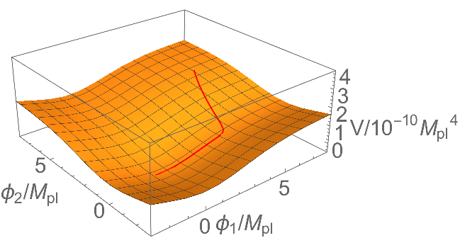
Figure 1: Left: The trajectory and the potential of T model. Right: Hubble parameter evolution of T model. The parameters are listed in Table 2.

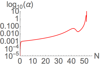
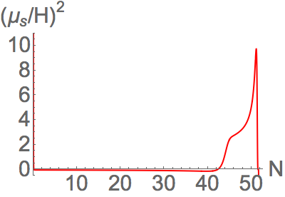
Figure 2: Left: $2$ times Turn rate per Hubble $\alpha=2\frac{\omega}{H}$ of T model. Right: Square mass of the entropic perturbation $\left(\frac{{\mu}_{s}}{H}\right)^{2}$ of T model. The parameters are listed in Table 2.

The possible parameter set of T model satisfying the e-folding constraint $50\leq{N}_{\text{end}}-{N}_{\text{hc}}\leq 60$ is listed in Table 2. From Figure 1, starting from a slope, the trajectory rolls down a nearly straight line to a valley along ${\phi}_{1}$ direction, turns significantly to move along the valley and then reaches the minimum point for oscillation. This significant turning is shown as a bump in the $\log_{10}{\left(\alpha\right)}-N$ graph in Figure 2 at about $42$ e-foldings since the speed of field evolution ${\sigma}^{\prime}$ drops at that point.

Apart from this, the square mass of the entropic perturbation $\left({\mu}_{s}/H\right)^{2}$, which is given by Eq.(129), is shown in Figure 2. One can see that before $42$ e-foldings, $\left({\mu}_{s}/H\right)^{2}$ remains small and negative. Since ${\mu}_{s}^{2}$ is related to the field curvature of the potential in the direction orthogonal to the trajectory, light and negative values mean that the field curvature orthogonal to the trajectory is light and negative so that the trajectory is rolling. At $42$ e-foldings, $\left({\mu}_{s}/H\right)^{2}$ surges since the trajectory turns to a valley, which means the field curvature becomes relatively large and positive. And finally, the trajectory runs to the minimum point for oscillation.

6.2 E model

$\Lambda/{M}_{\text{pl}}^{4}$	${\alpha}_{1}$	${\alpha}_{2}$	${m}_{1}/{M}_{\text{pl}}^{3}$	${m}_{2}/{M}_{\text{pl}}^{3}$	${n}_{1}$	${n}_{2}$	${\phi}_{1\text{ini}}/{M}_{\text{pl}}$
$0$	$2$	$2$	$1.1\times 10^{-5}$	$1\times 10^{-5}$	$1$	$1$	$5.8$
${\phi}_{2\text{ini}}/{M}_{\text{pl}}$	${\phi^{\prime}}_{1\text{ini}}/{M}_{\text{pl}}$	${\phi^{\prime}}_{2\text{ini}}/{M}_{\text{pl}}$	${N}_{\text{end}}$	${N}_{\text{stop}}$	${\beta}_{\text{iso}}$	$\cos{\Delta}$
$4.7$	$2\times 10^{-3}$	$2\times 10^{-3}$	$54.7826$	$56.9525$	$2.96101\times{10}^{-39}$	$0.168902$

Table 3: Parameters and initial conditions for a double field E model. ${N}_{\text{end}}$ is the number of e-foldings when ${\epsilon}_{H}=1$, while ${N}_{\text{stop}}$ is the number of e-foldings that we stop for numerical calculation. ${\beta}_{\text{iso}}$ and $\cos{\Delta}$ are defined in Eq.(142) and Eq.(141) respectively. Since the cosmological constant $\Lambda$ is small ($\Lambda\approx{10}^{-120}{M}_{\text{pl}}^{4}$), we can phenomenologically take $\Lambda=0$.

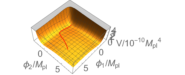
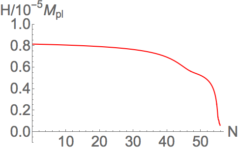
Figure 3: Left: The trajectory and the potential of E model. Right: Hubble parameter evolution of E model. The parameters are listed in Table 3.

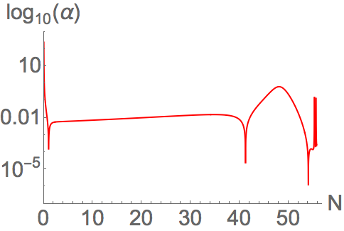
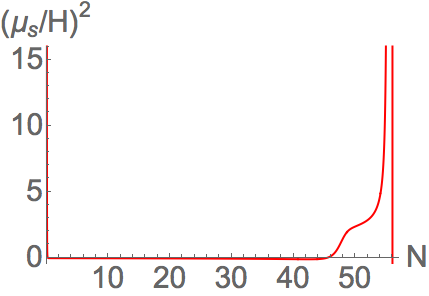
Figure 4: Left: $2$ times turn rate per Hubble $\alpha=2\frac{\omega}{H}$ of E model (in log scale). Right: Square mass of the entropic perturbation $\left(\frac{{\mu}_{s}}{H}\right)^{2}$ of E model. The parameters are listed in Table 3.

The possible parameter set of E model satisfying the e-folding constraint $50\leq{N}_{\text{end}}-{N}_{\text{hc}}\leq 60$ is listed in Table 3. From Figure 3, starting from a slope, the trajectory rolls down a nearly straight line to a valley along ${\phi}_{1}$ direction, turns significantly to move along the valley and then reaches the minimum point for oscillation. This significant turning is shown as a bump in the $\log_{10}{\left(\alpha\right)}-N$ graph in Figure 4 at about $48$ e-foldings since the the speed of field evolution ${\sigma}^{\prime}$ drops at that point.

Apart from this, the square mass of the entropic perturbation $\left({\mu}_{s}/H\right)^{2}$, which is given by Eq.(129), is shown in Figure 4. One can see that before $48$ e-foldings, $\left({\mu}_{s}/H\right)^{2}$ remains small and negative. Since ${\mu}_{s}^{2}$ is related to the field curvature of the potential in the direction orthogonal to the trajectory, light and negative values mean that the field curvature orthogonal to the trajectory is light and negative so that the trajectory is rolling. At $42$ e-foldings, $\left({\mu}_{s}/H\right)^{2}$ surges since the trajectory turns to a valley, which means the field curvature becomes relatively large and positive. And finally, the trajectory runs to the minimum point for oscillation.

7 Discussion

7.1 Similarity of T/E models and path dependence on initial conditions

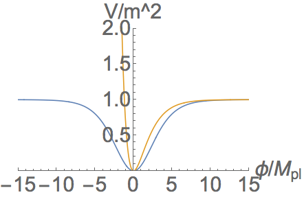
Figure 5: The $1$D potentials of $T$ and $E$ models (normalized by $m^{2}$). ($T$ model (blue): ${m}^{2}\tanh^{2p}{\left(\frac{\phi}{{M}_{\text{pl}}\sqrt{6{\alpha}}}\right)}$, $E$ model (yellow): ${m}^{2}\left(1-{e}^{-\sqrt{\frac{2}{3\alpha}}\frac{\phi}{{M}_{\text{pl}}}}\right)^{2p}$. In this figure, $\alpha=2$, $p=1$. )

We take two fields for the investigation to show the patterns of turning. Since the shapes of $T$ and $E$ models are very similar in the range of inflation (about $0\leq\phi\leq 6{M}_{\text{pl}}$) as we can see in Figure 5, and the corresponding kinetic terms are canonical, the physics of scalar fields in both models will be similar. In addition, the shape of the trajectory depends on the initial conditions. For instance, one may set the starting point with coordinates ${\phi}_{1}<{\phi}_{2}$. In that case, the trajectory slides along negative ${\phi}_{1}$ direction first and turns to the valley along ${\phi}_{2}$ direction instead to reach the minimum point.

7.2 An advantage of considering orthogonal nilpotent super-fields

In fact, these $T$ and $E$ models can be obtained by other motivations such as [18] and [20]. The difference between the approaches in [18] and [19] is that in the approach like [18], one needs to assume the mass scale of the associated part of the scalar field responsible for inflation is sufficiently heavy such that it is stabilized throughout the inflation process, while the approach of [19] provides a physical meaning to the sinflaton that its mass scale is very large. This gives a more physical reason for us to ignore the associated part of the scalar field, which makes us easier to construct potentials with more physical meanings.

7.3 Comments on the modified super-potential Eq.(73)

There are some comments pointing out that the $S$ components (real and imaginary parts) of the first derivatives evaluated at the minimum need not be zero because it is sufficient to consider the approximately zero of the first derivatives and $S$ can be written as a bilinear spinor form. Here our logic is the following. Since the origin of the orthogonal nilpotent constraints comes from the finite limits in the Lagrangian when the masses of sgoldstino, sinflaton and inflatino are very large, $S$ and $\text{Im}\left(\Phi\right)$ should be normally considered as scalar fields instead of the bilinear spinor forms before the E.O.M. calculation of super-fields. Since they are scalar fields, they should also be stabilized at the minimum. The minimum point of T model is $\left({Z}_{R},{Z}_{I},{S}_{R},{S}_{I}\right)=\left(0,0,0,0\right)$ while that of E model is $\left({T}_{R},{T}_{I},{S}_{R},{S}_{I}\right)=\left(1,0,0,0\right)$ and similar for multi-field versions. Thus, we consider whether there are some modifications to make the $S$ components of the first derivatives vanish, thereby showing the results above.

8 Conclusions

To conclude, our modification on the construction of T/E models can make all the components of the first derivative exactly zero at the minimum point. The modified part can be arbitrarily taken to obtain a physical cosmological constant. We also extend the modified T/E models into the multi-field versions by considering multi orthogonal nilpotent super-fields, whose sgoldstino, sinflatons and inflatinos are very heavy such that orthogonal nilpotent constraints are taken for the sake of obtaining physical limits. Finally, we study the double inflation dynamics of both T and E models respectively, and show their turning patterns, turning rate scales (about $O\left(0.1\right)$), the square mass of the entropic perturbation with scales $O\left(1\right)$ and relative transfer function $\cos{\Delta}$ with values $0.12$ and $0.169$ for T and E models respectively. These models can be further verified by updated observation data, and by considering other induced cosmological phenomena like the possibility of production of primordial black hole due to the trajectory turning [32, 33, 34, 35], which can be one of the directions of future work.

9 Ackonwledgement

The author thanks Prof. Hiroyuki ABE and Dr. Shuntaro Aoki very much for suggestion and useful discussions. The author is supported by Scholarship for Young Doctoral Students, Waseda University, Academic Year 2019.

Appendix A A review: Single orthogonal constrained field

A.1 A construction of T model

Basically, $\mathbb{S}$ and $\mathbb{\Phi}$ satisfying the nilpotent and orthogonality condition as

$$\mathbb{S}^{2}=0,\quad\mathbb{S}\mathbb{B}=0,\\$$ (57)

where $\mathbb{B}=\frac{1}{2i}\left(\mathbb{\Phi}-\overline{\mathbb{\Phi}}\right)$. The Kähler function $\mathcal{G}$ is given by

$$\mathcal{G}=-\frac{1}{2}\frac{3\alpha}{\left(1-Z\overline{Z}\right)^{2}}\left(Z-\overline{Z}\right)^{2}+\frac{\left|{W}_{0}\right|^{2}}{\left|{F}_{S}\right|^{2}+f\left(Z\overline{Z}\right)}S\overline{S}+S+\overline{S}+\ln{\left(\frac{\left|{W}_{0}\right|^{2}}{{M}_{\text{pl}}^{6}}\right)},\\$$ (58)

or equivalently, the Kähler potential and super-potential are

$$\frac{K}{{M}_{\text{pl}}^{2}}=-\frac{3{\alpha}}{2}\ln{\left[\frac{\left(1-Z\overline{Z}\right)^{2}}{\left(1-{Z}^{2}\right)\left(1-\overline{Z}^{2}\right)}\right]}+\frac{\left|{W}_{0}\right|^{2}}{\left|{F}_{S}\right|^{2}+f\left(Z\overline{Z}\right)}S\overline{S},\quad\quad W={W}_{0}{e}^{S},\\$$ (60)

The $F$ term potential is

$${V}_{F}:={M}_{\text{pl}}^{4}{e}^{\mathcal{G}}\left(\mathcal{G}^{{\alpha}\overline{\beta}}\mathcal{G}_{\alpha}\mathcal{G}_{\overline{\beta}}-3\right)={M}_{\text{pl}}^{-2}\left[\left|{F}_{S}\right|^{2}-3\left|{W}_{0}\right|^{2}+f\left({Z}^{2}\right)\right].\\$$ (61)

When we take $f\left(Z\overline{Z}\right)=m^{2}\left(Z\overline{Z}\right)^{n}$, in terms of a canonical field $\phi$, where $\text{Re}\left(Z\right)=\tanh{\left(\frac{\phi}{{M}_{\text{pl}}\sqrt{6{\alpha}}}\right)}$, we have

$${V}_{F}:=\frac{\left|{F}_{S}\right|^{2}-3\left|{W}_{0}\right|^{2}}{{M}_{\text{pl}}^{2}}+\frac{m^{2}}{{M}_{\text{pl}}^{2}}\tanh^{2n}{\left(\frac{\phi}{{M}_{\text{pl}}\sqrt{6{\alpha}}}\right)},\\$$ (62)

leading to the $T$ model potential given in [2]. In particular, the simple $T$ model described in [19] can be obtained by taking $n=1$.

A.2 A construction of E model

We impose the constraints

$$\mathbb{S}^{2}=0,\quad\mathbb{S}\left(\mathbb{T}-\overline{\mathbb{T}}\right)=0,\quad\Rightarrow\quad\left(\mathbb{T}-\overline{\mathbb{T}}\right)^{3}=0,\\$$ (63)

on the super-fields of the $E$ model. The Kähler function $\mathcal{G}$ is

$$\mathcal{G}=-\frac{1}{2}\frac{3{\alpha}}{\left(T+\overline{T}\right)^{2}}\left(T-\overline{T}\right)^{2}+\frac{\left|{W}_{0}\right|^{2}}{\left|{F}_{S}\right|^{2}+h\left(1-\frac{T+\overline{T}}{2}\right)}S\overline{S}+S+\overline{S}+\ln{\left(\frac{\left|{W}_{0}\right|^{2}}{{M}_{\text{pl}}^{6}}\right)},\\$$ (64)

or equivalently, the Kähler potential and super-potential are

$$\frac{K}{{M}_{\text{pl}}^{2}}=-\frac{3{\alpha}}{2}\ln{\left[\frac{\left(T+\overline{T}\right)^{2}}{4T\overline{T}}\right]}+\frac{\left|{W}_{0}\right|^{2}}{\left|{F}_{S}\right|^{2}+h\left(1-\frac{T+\overline{T}}{2}\right)}S\overline{S},\quad\quad W={W}_{0}{e}^{S}.\\$$ (66)

This $T$ parametrized Kähler potential can be obtained by taking the following Cayley transformation

$$T=\frac{Z+1}{-Z+1}\quad\Leftrightarrow\quad Z=\frac{T-1}{T+1},\\$$ (67)

from the $Z$ parametrized Kähler potential and vice versa without using the super-field constraints Eq.(57) and Eq.(63) since

$$-\frac{3{\alpha}}{2}\ln{\left[\frac{\left(1-Z\overline{Z}\right)^{2}}{\left(1-{Z}^{2}\right)\left(1-\overline{Z}^{2}\right)}\right]}=-\frac{3{\alpha}}{2}\ln{\left[\frac{\left(T+\overline{T}\right)^{2}}{4T\overline{T}}\right]}.\\$$ (68)

The $F$ term potential is

$${V}_{F}=\frac{\left|{F}_{S}\right|^{2}-3\left|{W}_{0}\right|^{2}}{{M}_{\text{pl}}^{2}}+\frac{1}{{M}_{\text{pl}}^{2}}h\left(1-\frac{T+\overline{T}}{2}\right),\\$$ (69)

or terms of a canonical field $\phi$, where $\text{Re}\left(T\right)={e}^{-\sqrt{\frac{2}{3\alpha}}\frac{\phi}{{M}_{\text{pl}}}}$,

$${V}_{F}=\frac{\left|{F}_{S}\right|^{2}-3\left|{W}_{0}\right|^{2}}{{M}_{\text{pl}}^{2}}+\frac{1}{{M}_{\text{pl}}^{2}}h\left(1-{e}^{-\sqrt{\frac{2}{3\alpha}}\frac{\phi}{{M}_{\text{pl}}}}\right),\\$$ (70)

By taking

$$h\left(1-\frac{T+\overline{T}}{2}\right)=m^{2}\left(1-\frac{T+\overline{T}}{2}\right)^{2n},\\$$ (71)

we obtain the $E$ model potential given in [2]

$${V}_{F}=\frac{\left|{F}_{S}\right|^{2}-3\left|{W}_{0}\right|^{2}}{{M}_{\text{pl}}^{2}}+\frac{m^{2}}{{M}_{\text{pl}}^{2}}\left(1-\frac{T+\overline{T}}{2}\right)^{2n}=\frac{\left|{F}_{S}\right|^{2}-3\left|{W}_{0}\right|^{2}}{{M}_{\text{pl}}^{2}}+\frac{m^{2}}{{M}_{\text{pl}}^{2}}\left(1-{e}^{-\sqrt{\frac{2}{3\alpha}}\frac{\phi}{{M}_{\text{pl}}}}\right)^{2n}.\\$$ (72)

In particular, the simple $E$ model described in [19] can be obtained by taking $n=1$.

Appendix B A derivation of the modified constant

We keep the original Kähler potential and modify the super-potential by adding a constant $k\in\mathbb{C}$ [26] as

$$W={W}_{0}e^{S}+k.\\$$ (73)

In this case, the $F$ term potential of T model at $S={Z}_{I}=0$ becomes

$${V}_{\text{T model}}=\frac{\left|{F}_{S}\right|^{2}-3\left|{W}_{0}+k\right|^{2}}{{M}_{\text{pl}}^{2}}+\frac{f\left({Z}_{R}^{2}\right)}{{M}_{\text{pl}}^{2}},\\$$ (74)

and its first derivative evaluated at the minimum point becomes

$${M}_{\text{pl}}^{-2}\{0,0,2[\left|{F}_{S}\right|^{2}-2\left|{W}_{0}\right|^{2}-2\text{Re}\left(\overline{{W}_{0}}k\right)+f(0)],-4\text{Im}\left(\overline{{W}_{0}}k\right)\}.\\$$ (75)

We can see that

$$\begin{split}\text{Im}\left(\overline{{W}_{0}}k\right)=&\;0,\\ \left|{F}_{S}\right|^{2}-3\left|{W}_{0}+k\right|^{2}=&\;{M}_{\text{pl}}^{2}\Lambda,\\ \left|{F}_{S}\right|^{2}-2\left|{W}_{0}\right|^{2}-2\text{Re}\left(\overline{{W}_{0}}k\right)=&\;0.\\ \end{split}$$ (76)

On solving, we obtain

$$\begin{split}\Lambda=&\;-\frac{\overline{W}_{0}}{{W}_{0}}\frac{\left({W}_{0}+k\right)\left({W}_{0}+3k\right)}{{M}_{\text{pl}}^{2}},\\ \left|{F}_{S}\right|^{2}=&\;2\left(k+{W}_{0}\right)\overline{{W}_{0}}.\\ \end{split}$$ (77)

If $-{W}_{0}<k\leq-\frac{1}{3}{W}_{0}$, we can attain the dS spacetime, and accordingly, all the first derivatives can be zero provided that $\left|{F}_{S}\right|^{2}=2\left(k+{W}_{0}\right)\overline{{W}_{0}}$. For example, when we take $k=-\frac{2}{3}{W}_{0}$, we obtain $\Lambda=\frac{1}{3}\frac{\left|{W}_{0}\right|^{2}}{{M}_{\text{pl}}^{2}}$ and $\left|{F}_{S}\right|^{2}=\frac{2}{3}\left|{W}_{0}\right|^{2}$. Hence, this can be applicable when $\Lambda$, $\left|{W}_{0}\right|^{2}$ and $\left|{F}_{S}\right|^{2}$ have the same scale. Interestingly, when we take $k$ sufficiently close to $-\frac{1}{3}{W}_{0}$, say, $k=-\left(\delta+\frac{1}{3}\right){W}_{0}$ with sufficiently small $\delta>0$, we obtain $\Lambda=\delta\left(2-3\delta\right)\frac{\left|{W}_{0}\right|^{2}}{{M}_{\text{pl}}^{2}}$ and $\left|{F}_{S}\right|^{2}=\frac{2}{3}\left(2-3\delta\right)\left|{W}_{0}\right|^{2}$. The smallness of $\delta$ can be responsible for that of $\Lambda$, and allow arbitrary scales for $\left|{W}_{0}\right|^{2}$ and $\left|{F}_{S}\right|^{2}$. This implies when $\delta$ is sufficiently small, it can allow $\left|{W}_{0}\right|^{2}$ and $\left|{F}_{S}\right|^{2}$ much larger than $\Lambda$, while $\delta$ can have a scale $O\left(0.1\right)$ with $\delta<\frac{2}{3}$ when $\left|{W}_{0}\right|^{2}$ and $\left|{F}_{S}\right|^{2}$ are compatible with $\Lambda$. Thus, without loss of generality, we take $k=-(\delta+\frac{1}{3}){W}_{0}$ with $\delta>0$ for discussion. We can also solve the problem in E model by this trick. The $F$ term potential of E model at $S={T}_{I}=0$ becomes

$${V}_{\text{E model}}=\frac{\left|{F}_{S}\right|^{2}-3\left|{W}_{0}+k\right|^{2}}{{M}_{\text{pl}}^{2}}+\frac{h\left(1-{T}_{R}\right)}{{M}_{\text{pl}}^{2}},\\$$ (78)

and its first derivative evaluated at the minimum point becomes

$${M}_{\text{pl}}^{-2}\left\{0,0,2\left[\left|{F}_{S}\right|^{2}-2\left|{W}_{0}\right|^{2}-2\text{Re}\left(\overline{{W}_{0}}k\right)+h(0)\right],-4\text{Im}\left(\overline{{W}_{0}}k\right)\right\}.\\$$ (79)

By repeating the same procedures above, we can obtain the same result. Next, we extend these two models into multi-field cases.

Appendix C A formalism of Double Field Inflation

In this section, we follow the derivation in [29] and [30]. For a recent application, please refer to [31]. The action in Jordan frame is

$${S}_{\text{Jordan}}=\int d^{4}x\sqrt{-\tilde{g}}\left[f\left({\phi}^{I}\right)\tilde{R}-\frac{1}{2}\tilde{\mathcal{G}}_{IJ}\tilde{g}^{{\mu}{\nu}}\tilde{\triangledown}_{\mu}{\phi}^{I}\tilde{\triangledown}_{\nu}{\phi}^{J}-\tilde{V}\left({\phi}^{I}\right)\right].\\$$ (80)

where $f\left({\phi}^{I}\right)$ is the non-minimal coupling function and $\tilde{V}\left({\phi}^{I}\right)$ is the potential for the scalar fields in Jordan frame. To change the action in Jordan frame into the counterpart in Einstein frame, we define a spacetime metric in Einstein frame ${g}_{{\mu}{\nu}}\left(x\right)$ as

$${g}_{{\mu}{\nu}}\left(x\right)={\Omega}^{2}\left(x\right)\tilde{g}_{{\mu}{\nu}}\left(x\right),\\$$ (81)

where the conformal factor ${\Omega}^{2}\left(x\right)$ is given by

$${\Omega}^{2}\left(x\right)=\frac{2}{{M}^{2}_{\text{pl}}}f\left({\phi}^{I}\left(x\right)\right).\\$$ (82)

Then, the action in Jordan frame becomes that in Einstein frame, which is given by

$${S}_{\text{Einstein}}=\int d^{4}x\sqrt{-{g}}\left[\frac{{M}^{2}_{\text{pl}}}{2}{R}-\frac{1}{2}{\mathcal{G}}_{IJ}{g}^{{\mu}{\nu}}{\triangledown}_{\mu}{\phi}^{I}{\triangledown}_{\nu}{\phi}^{J}-{V}\left({\phi}^{I}\right)\right].\\$$ (83)

The potential in Einstein frame becomes

$$V\left({\phi}^{I}\right)=\frac{\tilde{V}\left({\phi}^{I}\right)}{{\Omega}^{4}\left(x\right)}=\frac{{M}^{4}_{\text{pl}}}{4f^{2}\left({\phi}^{I}\right)}\tilde{V}\left({\phi}^{I}\right).\\$$ (84)

The coefficients $\mathcal{G}_{{I}{J}}$ of the non-canonical kinetic terms in Einstein frame depend on the non-minimal coupling function $f\left({\phi}^{I}\right)$ and its derivatives. They are given by

$$\mathcal{G}_{{I}{J}}\left({\phi}^{K}\right)=\frac{{M}^{2}_{\text{pl}}}{2f\left({\phi}^{L}\right)}\left[\tilde{\mathcal{G}}_{{I}{J}}\left({\phi}^{K}\right)+\frac{3}{f\left({\phi}^{L}\right)}{f}_{,I}{f}_{,J}\right],\\$$ (85)

where ${f}_{,I}=\frac{{\partial}{f}}{{\partial}{\phi}^{I}}$. Varying the action in Einstein frame with respect to ${g}_{{\mu}{\nu}}\left(x\right)$, we have Einstein equations

$${R}_{{\mu}{\nu}}-\frac{1}{2}{g}_{{\mu}{\nu}}R=\frac{1}{{M}^{2}_{\text{pl}}}{T}_{{\mu}{\nu}},\\$$ (86)

where

$${T}_{{\mu}{\nu}}=\mathcal{G}_{{I}{J}}{\partial}_{\mu}{\phi}^{I}{\partial}_{\nu}{\phi}^{J}-{g}_{{\mu}{\nu}}\left[\frac{1}{2}\mathcal{G}_{{K}{L}}{\partial}_{\gamma}{\phi}^{K}{\partial}^{\gamma}{\phi}^{L}+V\left({\phi}^{K}\right)\right].\\$$ (87)

Varying Eq. (83) with respect to ${\phi}^{I}$, we obtain the equation of motion for ${\phi}^{I}$

$$\square{\phi}^{I}+{g}^{{\mu}{\nu}}{\Gamma}^{I}_{{J}{K}}{\partial}_{\mu}{\phi}^{J}{\partial}_{\nu}{\phi}^{K}-\mathcal{G}^{{I}{K}}{V}_{,K}=0,\\$$ (88)

where $\square{\phi}^{I}={g}^{{\mu}{\nu}}{\phi}^{I}_{;{\mu}{\nu}}$ and ${\Gamma}^{I}_{{J}{K}}$ is the Christoffel symbol for the field space manifold in terms of $\mathcal{G}_{{I}{J}}$ and its derivatives. We expand each scalar field to the first order around its classical background value,

$${\phi}^{I}\left({x}^{\mu}\right)={\varphi}^{I}\left(t\right)+{\delta}{\phi}^{I}\left({x}^{\mu}\right),\\$$ (89)

and perturb a spatially flat Friedmann-Robertson-Walker (FRW) metric,

$$ds^{2}={g}_{{\mu}{\nu}}d{x}^{\mu}d{x}^{\nu}=-\left(1+2A\right)dt^{2}+2a\left({\partial}_{i}B\right)d{x}^{i}dt+a^{2}\left[\left(1-2{\psi}\right){\delta}_{ij}+2{\partial}_{i}{\partial}_{j}E\right]d{x}^{i}d{x}^{j},\\$$ (90)

where $a\left(t\right)$ is the scale factor. To the zeroth order, the $00$ and $ij$ components of Einstein equations become

$$H^{2}=\frac{1}{3{M}^{2}_{\text{pl}}}\left[\frac{1}{2}\mathcal{G}_{{I}{J}}\dot{\varphi}^{I}\dot{\varphi}^{J}+V\left({\varphi}^{I}\right)\right],\\$$ (91)

$$\dot{H}=-\frac{1}{2{M}^{2}_{\text{pl}}}\mathcal{G}_{{I}{J}}\dot{\varphi}^{I}\dot{\varphi}^{J},\\$$ (92)

where $H=\frac{\dot{a}\left(t\right)}{a\left(t\right)}$ is the Hubble parameter, and the field field space metric is calculated at the zeroth order, $\mathcal{G}_{{I}{J}}=\mathcal{G}_{{I}{J}}\left({\varphi}^{K}\right)$. In terms of the number of e-foldings $N=\ln{a}$ with $dN=Hdt$, the above Einstein equation becomes

$$3{M}^{2}_{\text{pl}}-\frac{1}{2}\mathcal{G}_{{I}{J}}{{\varphi}^{I}}^{\prime}{{\varphi}^{J}}^{\prime}=\frac{V\left({\varphi}^{I}\right)}{H^{2}},\\$$ (93)

$$\frac{H^{\prime}}{H}=-\frac{1}{2{M}^{2}_{\text{pl}}}\mathcal{G}_{{I}{J}}{{\varphi}^{I}}^{\prime}{{\varphi}^{J}}^{\prime},\\$$ (94)

where the prime ^′ means the derivative with respect to $N$. For any vector in the field space $A^{I}$, we define a covariant derivative with respect to the field-space metric as usual by

$$\mathcal{D}_{J}{A}^{I}={\partial}_{J}{A}^{I}+{\Gamma}^{I}_{{J}{K}}{A}^{K},\\$$ (95)

and the time derivative with respect to the cosmic time $t$ is given by

$$\mathcal{D}_{t}{A}^{I}\equiv\dot{\varphi}^{J}\mathcal{D}_{J}{A}^{I}=\dot{A}^{I}+{\Gamma}^{I}_{{J}{K}}\dot{\varphi}^{J}{A}^{K}=H\left({{A}^{I}}^{\prime}+{\Gamma}^{I}_{{J}{K}}{{\varphi}^{J}}^{\prime}{A}^{K}\right).\\$$ (96)

Now, we define the length of the velocity vector for the background fields as

$$|\dot{\varphi}^{I}|\equiv\dot{\sigma}=\sqrt{\mathcal{G}_{{P}{Q}}\dot{\varphi}^{P}\dot{\varphi}^{Q}}\quad\Rightarrow\quad|{{\varphi}^{I}}^{\prime}|\equiv{\sigma}^{\prime}=\sqrt{\mathcal{G}_{{P}{Q}}{{\varphi}^{P}}^{\prime}{{\varphi}^{Q}}^{\prime}}.$$ (97)

After introducing the unit vector of the velocity vector of the background fields

$$\hat{\sigma}^{I}\equiv\frac{\dot{\varphi}^{I}}{\dot{\sigma}}=\frac{{{\varphi}^{I}}^{\prime}}{{\sigma}^{\prime}}=\frac{{{\varphi}^{I}}^{\prime}}{\sqrt{\mathcal{G}_{{P}{Q}}{{\varphi}^{P}}^{\prime}{{\varphi}^{Q}}^{\prime}}},\\$$ (98)

the $00$ and $ij$ components of Einstein equations become

$$H^{2}=\frac{1}{3{M}^{2}_{\text{pl}}}\left[\frac{1}{2}\dot{\sigma}^{2}+V\right]\quad\Leftrightarrow\quad 3{M}^{2}_{\text{pl}}-\frac{1}{2}{{\sigma}^{\prime}}^{2}=\frac{V\left({\varphi}^{I}\right)}{H^{2}}\quad\Leftrightarrow\quad\frac{V}{{M}_{\text{pl}}^{2}H^{2}}=\left(3-{\epsilon}_{H}\right),\\$$ (99)

$$\dot{H}=-\frac{1}{2{M}^{2}_{\text{pl}}}\dot{\sigma}^{2}\quad\Leftrightarrow\quad\frac{H^{\prime}}{H}=-\frac{1}{2{M}^{2}_{\text{pl}}}{{\sigma}^{\prime}}^{2}\quad\Leftrightarrow\quad\frac{{{\sigma}^{\prime}}^{2}}{{M}_{\text{pl}}^{2}}=\frac{\dot{\sigma}^{2}}{{M}_{\text{pl}}^{2}H^{2}}=2{\epsilon}_{H},\\$$ (100)

and the equation of motion of ${\phi}^{I}$ in the zeroth order is

$$\ddot{\sigma}+3H\dot{\sigma}+{V}_{,\sigma}=0\quad\Leftrightarrow\quad\frac{\ddot{\sigma}}{H\dot{\sigma}}=-3-\frac{3-{\epsilon}_{H}}{2{\epsilon}_{H}}\frac{d}{dN}\left(\ln{V}\right),\\$$ (101)

where

$${V}_{,\sigma}\equiv\hat{\sigma}^{I}{V}_{,I}.\\$$ (102)

and ${\epsilon}_{H}$ is the first order Hubble slow-roll parameter defined in Eq.(105). We define a quantity $\hat{s}^{{I}{J}}$

$$\hat{s}^{{I}{J}}\equiv\mathcal{G}^{{I}{J}}-\hat{\sigma}^{I}\hat{\sigma}^{J},\\$$ (103)

which obeys the following relations with $\hat{\sigma}^{I}$

$$\begin{split}\hat{\sigma}_{I}\hat{\sigma}^{I}=1,\\ \hat{s}^{{I}{J}}\hat{s}_{{I}{J}}=\mathcal{N}-1,\\ \hat{s}^{I}_{\;A}\hat{s}^{A}_{\;J}=\hat{s}^{I}_{\;J},\\ \hat{\sigma}_{I}\hat{s}^{{I}{J}}=0\quad\forall J.\\ \end{split}$$ (104)

The slow-roll parameters are given by

$${\epsilon}_{H}\equiv-\frac{\dot{H}}{H^{2}}=\frac{3\dot{\sigma}^{2}}{\dot{\sigma}^{2}+2V}\quad\Leftrightarrow\quad\frac{\dot{\sigma}^{2}}{V}=\frac{2{\epsilon}_{H}}{3-{\epsilon}_{H}},\\$$ (105)

and

$${\eta}_{{\sigma}{\sigma}}\equiv{M}^{2}_{\text{pl}}\frac{\mathcal{M}_{{\sigma}{\sigma}}}{V}\quad\text{and}\quad{\eta}_{{s}{s}}\equiv{M}^{2}_{\text{pl}}\frac{\mathcal{M}_{{s}{s}}}{V},\\$$ (106)

where $\mathcal{M}^{I}_{J}$ is the effective mass squared matrix given by

$$\begin{split}{\mathcal{M}}^{I}_{J}\equiv&\;\mathcal{G}^{IK}\left(\mathcal{D}_{J}\mathcal{D}_{K}V\right)-\mathcal{R}^{I}_{LMJ}\dot{\varphi}^{L}\dot{\varphi}^{M},\\ {\mathcal{M}}_{{\sigma}{J}}\equiv&\;\hat{\sigma}_{I}\mathcal{M}^{I}_{J}=\hat{\sigma}^{K}\left(\mathcal{D}_{K}\mathcal{D}_{J}V\right),\\ {\mathcal{M}}_{{\sigma}{\sigma}}\equiv&\;\hat{\sigma}_{I}\hat{\sigma}^{J}\mathcal{M}^{I}_{J}=\hat{\sigma}^{K}\hat{\sigma}^{J}\left(\mathcal{D}_{K}\mathcal{D}_{J}V\right),\\ {\mathcal{M}}_{{s}{J}}\equiv&\;\hat{s}_{I}\mathcal{M}^{I}_{J}=\hat{s}_{I}\left(\mathcal{G}^{IK}\left(\mathcal{D}_{J}\mathcal{D}_{K}V\right)-\mathcal{R}^{I}_{LMJ}\dot{\varphi}^{L}\dot{\varphi}^{M}\right),\\ {\mathcal{M}}_{{s}{s}}\equiv&\;\hat{s}_{I}\hat{s}^{J}\mathcal{M}^{I}_{J}=\hat{s}_{I}\hat{s}^{J}\left(\mathcal{G}^{IK}\left(\mathcal{D}_{J}\mathcal{D}_{K}V\right)-\mathcal{R}^{I}_{LMJ}\dot{\varphi}^{L}\dot{\varphi}^{M}\right),\\ \end{split}$$ (107)

and $\hat{s}^{I}$ is defined in Eq.(111). We define the turn-rate vector ${\omega}^{I}$ as the covariant rate of change of the unit vector $\hat{\sigma}^{I}$ and its square norm

$${\omega}^{I}\equiv\mathcal{D}_{t}\hat{\sigma}^{I}=-\frac{1}{\dot{\sigma}}{V}_{,K}\hat{s}^{{I}{K}}=\frac{-1}{H{\sigma}^{\prime}}{V}_{,K}\hat{s}^{{I}{K}},\quad\quad{\omega}^{2}:={\omega}_{L}{\omega}^{L}=\frac{1}{\dot{\sigma}^{2}}\left[{V}_{,L}{V}^{,L}-{V}_{,{\sigma}}^{2}\right].\\$$ (108)

Since ${\omega}^{I}\propto\hat{s}^{{I}{K}}$, we have

$${\omega}^{I}\hat{\sigma}_{I}=0.\\$$ (109)

We can also find

$$\mathcal{D}_{t}\hat{s}^{{I}{J}}=-\hat{\sigma}^{I}{\omega}^{J}-\hat{\sigma}^{J}{\omega}^{I}.\\$$ (110)

Also, we introduce a new unit vector $\hat{s}^{I}$ pointing in the direction of the turn-rate, ${\omega}^{I}$, and a new projection operator ${\gamma}^{{I}{J}}$

$$\hat{s}^{I}\equiv\frac{{\omega}^{I}}{\omega},\\$$ (111)

$${\gamma}^{{I}{J}}\equiv{\mathcal{G}}^{{I}{J}}-\hat{\sigma}^{I}\hat{\sigma}^{J}-\hat{s}^{I}\hat{s}^{J}.\\$$ (112)

where ${\omega}=|{\omega}^{I}|$ is the magnitude of the turn-rate vector. The new unit vector $\hat{s}^{I}$ and the new projection operator ${\gamma}^{{I}{J}}$ also satisfy

$$\begin{split}\hat{s}^{{I}{J}}=&\hat{s}^{I}\hat{s}^{J}+{\gamma}^{{I}{J}},\\ {\gamma}^{{I}{J}}{\gamma}_{{I}{J}}=&\mathcal{N}-2,\\ \hat{s}^{{I}{J}}\hat{s}_{J}=&\hat{s}^{I},\\ \hat{\sigma}_{I}\hat{s}^{I}=&\hat{\sigma}_{I}{\gamma}^{{I}{J}}=\hat{s}_{I}{\gamma}^{{I}{J}}=0\quad\forall J.\end{split}$$ (113)

We then find

$${\mathcal{D}}_{t}\hat{s}^{I}=-{\omega}\hat{\sigma}^{I}-{\Pi}^{I},\\ {\mathcal{D}}_{t}{\gamma}^{{I}{J}}=\hat{s}^{I}{\gamma}^{J}+\hat{s}^{J}{\gamma}^{I},\\$$ (114)

where

$${\Pi}^{I}\equiv\frac{1}{\omega}{\mathcal{M}}_{{\sigma}{K}}{\gamma}^{{I}{K}},\\$$ (115)

and hence

$$\hat{\sigma}_{I}{\Pi}^{I}=\hat{s}_{I}{\Pi}^{I}=0.\\$$ (116)

Now, we define the curvature and entropic perturbations as follows

$$\mathcal{R}={\psi}+\frac{H}{\dot{\sigma}}\hat{\sigma}_{J}{\delta}{\phi}^{J}=\frac{H}{\dot{\sigma}}{Q}_{\sigma},\\$$ (117)

$$\mathcal{S}=\frac{H}{\dot{\sigma}}{Q}_{s},\\$$ (118)

whose E.O.M.s are given by [30]

$$\begin{split}\ddot{Q}_{\sigma}+3H\dot{Q}_{\sigma}+\left[\left(\frac{k}{a}\right)^{2}+\mathcal{M}_{{\sigma}{\sigma}}-{\omega}^{2}-\frac{1}{{M}_{\text{pl}}^{2}a^{3}}\frac{d}{dt}\left(\frac{a^{3}\dot{\sigma}^{2}}{H}\right)\right]{Q}_{\sigma}=&\;2\frac{d}{dt}\left({\omega}{Q}_{s}\right)-2\left(\frac{{V}_{,\sigma}}{\dot{\sigma}}+\frac{\dot{H}}{H}\right){\omega}{Q}_{s},\\ \ddot{Q}_{s}+3H\dot{Q}_{s}+\left[\left(\frac{k}{a}\right)^{2}+\mathcal{M}_{ss}+3{\omega}^{2}\right]{Q}_{s}=&\;4{M}_{\text{pl}}^{2}\frac{\omega}{\dot{\sigma}}\frac{k^{2}}{a^{2}}{\Psi},\\ \end{split}$$ (119)

where $\Psi$ is the gauge-invariant Bardeen potential [27, 28], $\mathcal{M}_{{\sigma}{\sigma}}$ and $\mathcal{M}_{ss}$ are given by Eq.(107) and

$${\mu}_{s}^{2}=\mathcal{M}_{ss}+3{\omega}^{2},\\$$ (120)

is the (effective) square mass of entropic perturbations. After the first horizon crossing, the co-moving wave number $k$ obeys $\frac{k}{aH}<1$. Hence, the curvature and entropic perturbations satisfy the following equations

$$\dot{\mathcal{R}}={\alpha}H\mathcal{S}+O\left(\frac{k^{2}}{a^{2}H^{2}}\right),\\$$ (121)

$$\dot{\mathcal{S}}={\beta}H\mathcal{S}+O\left(\frac{k^{2}}{a^{2}H^{2}}\right),\\$$ (122)

which allow us to write the transfer functions

$${T}_{\mathcal{RS}}\left({t}_{\text{hc}},t\right)=\int^{t}_{{t}_{\text{hc}}}d{t}^{\prime}{\alpha}\left(t^{\prime}\right)H\left(t^{\prime}\right){T}_{\mathcal{SS}}\left({t}_{\text{hc}},t^{\prime}\right),\\$$ (123)

$${T}_{\mathcal{SS}}\left({t}_{\text{hc}},t\right)=\exp\left[\int^{t}_{{t}_{\text{hc}}}{dt^{\prime}}{\beta}\left(t^{\prime}\right)H\left(t^{\prime}\right)\right],\\$$ (124)

where ${t}_{\text{hc}}$ is the time of the first horizon crossing. Being changed from the cosmic time $t$ into the number of e-foldings $N$, ${T}_{\mathcal{RS}}\left({t}_{\text{hc}},t\right)$ and ${T}_{\mathcal{SS}}\left({t}_{\text{hc}},t\right)$ become

$${T}_{\mathcal{RS}}\left({N}_{\text{hc}},N\right)=\int^{N}_{{N}_{\text{hc}}}{dN^{\prime}}{\alpha}\left(N^{\prime}\right){T}_{\mathcal{SS}}\left({N}_{\text{hc}},N^{\prime}\right),\\$$ (125)

and

$${T}_{\mathcal{SS}}\left({N}_{\text{hc}},N\right)=\exp\left[\int^{N}_{{N}_{\text{hc}}}{dN^{\prime}}{\beta}\left(N^{\prime}\right)\right].\\$$ (126)

The E.O.M.s of curvature and entropic perturbations are [29]

$$\dot{\mathcal{R}}=2{\omega}\mathcal{S}+O\left(\frac{k^{2}}{a^{2}H^{2}}\right),\\$$ (127)

and

$$\dot{Q}_{s}\simeq-\frac{{\mu}^{2}_{s}}{3H}{Q}_{s},\\$$ (128)

where the square mass of entropic perturbation can be written as

$${\mu}^{2}_{s}={\mathcal{M}}_{ss}+3{\omega}^{2}\quad\Leftrightarrow\quad\frac{{\mu}^{2}_{s}}{H^{2}}=\left(3-{\epsilon}\right){\eta}_{ss}+\frac{3}{4}{\alpha}^{2},\\$$ (129)

and $\simeq$ means slow-roll approximation and ${\alpha}$ is given in Eq.(130). Comparing with Eq.(117), (118), (121) and (122) with Eq.(127) and (128) [29], we obtain

$${\alpha}\left(t\right)=\frac{2{\omega}\left(t\right)}{H\left(t\right)}\quad\Leftrightarrow\quad{\alpha}\left(N\right)=\frac{2{\omega}\left(N\right)}{H\left(N\right)},\\$$ (130)

and

$${\beta}=-\frac{{\mu}^{2}_{s}}{3H^{2}}-{\epsilon}-\frac{\ddot{\sigma}}{H\dot{\sigma}}=-{\eta}_{ss}\left(1-\frac{1}{3}{\epsilon}\right)+\left(3-{\epsilon}\right)+\frac{3-{\epsilon}}{2{\epsilon}}\frac{d}{dN}\left({\ln{V}}\right)-\frac{1}{4}{\alpha}^{2},\\$$ (131)

The power spectrum for the gauge invariant curvature perturbation is given by

$$\langle\mathcal{R}\left(\mathbb{k}_{1}\right)\mathcal{R}\left(\mathbb{k}_{2}\right)\rangle=\left(2\pi\right)^{3}{\delta}^{\left(3\right)}\left(\mathbb{k}_{1}+\mathbb{k}_{2}\right){P}_{\mathcal{R}}\left({k}_{1}\right),\\$$ (132)

where ${P}_{\mathcal{R}}\left(k\right)=|\mathcal{R}|^{2}$. The dimensionless power spectrum is

$${\mathcal{P}}_{\mathcal{R}}=\frac{k^{3}}{2{\pi}^{2}}|\mathcal{R}|^{2},\\$$ (133)

and the spectral index is defined as

$${n}_{s}\equiv 1+\left.\frac{d\ln{\mathcal{P}}_{\mathcal{R}}}{d\ln{k}}\right|_{\text{hc}},\\$$ (134)

where $k$ is the pivot scale and hc means the first horizon crossing. Using the transfer function, we can relate the power spectra of adiabatic and entropic perturbations at time ${t}_{\text{hc}}$ to their values at some later time $t>{t}_{\text{hc}}$ with the corresponding pivot scale $k$ as

$$\begin{split}{\mathcal{P}}_{\mathcal{R}}\left(k\right)=&\;{\mathcal{P}}_{\mathcal{R}}\left({k}_{\text{hc}}\right)\left[1+{T}^{2}_{\mathcal{RS}}\left({t}_{\text{hc}},t\right)\right],\\ {\mathcal{P}}_{\mathcal{S}}\left(k\right)=&\;{\mathcal{P}}_{\mathcal{R}}\left({k}_{\text{hc}}\right){T}^{2}_{\mathcal{SS}}\left({t}_{\text{hc}},t\right).\\ \end{split}$$ (136)

The transfer functions satisfy

$$\begin{split}\frac{1}{H\left({t}_{\text{hc}}\right)}\frac{{\partial}{T}_{\mathcal{RS}}\left({t}_{\text{hc}},t\right)}{{\partial}{t}_{\text{hc}}}&=\;-{\alpha}\left({t}_{\text{hc}}\right)-{\beta}\left({t}_{\text{hc}}\right){T}_{\mathcal{SS}}\left({t}_{\text{hc}},{t}\right),\\ \frac{1}{H\left({t}_{\text{hc}}\right)}\frac{{\partial}{T}_{\mathcal{SS}}\left({t}_{\text{hc}},t\right)}{{\partial}{t}_{\text{hc}}}&=\;-{\beta}\left({t}_{\text{hc}}\right){T}_{\mathcal{SS}}\left({t}_{\text{hc}},t\right).\\ \end{split}$$ (137)

In term of the number of e-foldings $N$, the above differential equations become

$$\begin{split}\frac{{\partial}{T}_{\mathcal{RS}}\left({N}_{\text{hc}},N\right)}{{\partial}{N}_{\text{hc}}}&=\;-{\alpha}\left({N}_{\text{hc}}\right)-{\beta}\left({N}_{\text{hc}}\right){T}_{\mathcal{SS}}\left({N}_{\text{hc}},N\right),\\ \frac{{\partial}{T}_{\mathcal{SS}}\left({N}_{\text{hc}},N\right)}{{\partial}{N}_{\text{hc}}}&=\;-{\beta}\left({N}_{\text{hc}}\right){T}_{\mathcal{SS}}\left({N}_{\text{hc}},N\right).\\ \end{split}$$ (138)

The spectral index for the power spectrum of the adiabatic fluctuations becomes

$${n}_{s}\simeq{n}_{s}\left({t}_{\text{hc}}\right)+\frac{1}{H}\left(\frac{{\partial}{T}_{\mathcal{RS}}}{{\partial}{t}_{\text{hc}}}\right)\sin{2\Delta},\\$$ (139)

where

$${n}_{s}\left({t}_{\text{hc}}\right)=1-6{\epsilon}_{H}\left({t}_{\text{hc}}\right)+2{\eta}_{{\sigma}{\sigma}}\left({t}_{\text{hc}}\right),\\$$ (140)

and the trigonometric functions for ${T}_{\mathcal{RS}}$ are defined as

$$\sin{\Delta}\equiv\;\frac{1}{\sqrt{1+T^{2}_{\mathcal{RS}}}},\quad\cos{\Delta}\equiv\frac{{T}_{\mathcal{RS}}}{\sqrt{1+{T}^{2}_{\mathcal{RS}}}},\quad\tan{\Delta}\equiv\;\frac{1}{T_{\mathcal{RS}}}.\\$$ (141)

The iso-curvature fraction is given by

$${\beta}_{\text{iso}}\equiv\frac{{\mathcal{P}}_{\mathcal{S}}}{{\mathcal{P}}_{\mathcal{R}}+{\mathcal{P}}_{\mathcal{S}}}=\frac{T^{2}_{\mathcal{SS}}}{1+T^{2}_{\mathcal{SS}}+T^{2}_{\mathcal{RS}}},\\$$ (142)

which can be used for comparing the predictions with the recent observation data. Also, the tensor-to-scalar ratio is given by

$$r\simeq\frac{16{\epsilon}}{1+T^{2}_{\mathcal{RS}}}.\\$$ (143)

References

- [1] F. Farakos, A. Kehagias, A. Riottob, On the Starobinsky model of inflation from supergravity, Nuclear Physics Volume 876, Issue 1, 2013, page 187 - 200, arXiv: 1307.1137
- [2] Planck Collaboration, Planck 2018 results. X. Constraints on inflation, arXiv: 1807.06211
- [3] D. V. Volkov and V. P. Akulov, Possible universal neutrino interaction, Journal of Experimental and Theoretical Physics Letter 16 (1972), 438 - 440.
- [4] M. Rocek, Linearizing the Volkov - Akulov Model, Physical Review Letter 41 (1978), 451 - 453.
- [5] Z. Komargodski and N. Seiberg, From Linear SUSY to Constrained Superfields, Journal of High Energy Physics 09 (2009) 066, arXiv: 0907.2441
- [6] Renata Kallosh, Anna Karlsson, Divyanshu Murli, From Linear to Non-linear Supersymmetry via Functional Integration, Physical Review D 93, 025012 (2016), arXiv: 1511.07547
- [7] F. Hasegawa and Y. Yamada, Component action of nilpotent multiplet coupled to matter in dimensional supergravity, Journal of High Energy Physics 10 (2015) 106, arXiv: 1507.08619
- [8] Eric A. Bergshoeff, Daniel Z. Freedman, Renata Kallosh, Antoine Van Proeyen, Pure de Sitter Supergravity, Physical Review D 92 085040, 2015, arXiv: 1507.08264
- [9] Renata Kallosh, Matter-coupled de Sitter Supergravity, Theoretical and Mathematical Physics volume 187, pages 695-705 (2016), arXiv: 1509.02136
- [10] Renata Kallosh, Timm Wrase, De Sitter Supergravity Model Building, Physical Review D 92, 105010 (2015), arXiv: 1509.02137
- [11] I. Antoniadis, E. Dudas, S. Ferrara, A. Sagnotti, The Volkov - Akulov - Starobinsky Supergravity, Physics Letter B Volume 733 (2014) Pages 32-35, arXiv: 1403.3269
- [12] Sergio Ferrara, Renata Kallosh and Andrei Linde, Cosmology with Nilpotent Superfields, Journal of High Energy Physics 10 143, 2014, arXiv: 1408.4096
- [13] G. Dall’Agata and F. Zwirner, On sgoldstino - less supergravity models of inflation, Journal of High Energy Physics 12 (2014) 172, arXiv: 1411.2605
- [14] Gianguido Dall’Agata, Sergio Ferrara, Fabio Zwirner, Minimal scalar-less matter-coupled supergravity, Physics Letters B 752 (2016) 263-266, arXiv: 1509.06345
- [15] Sergio Ferrara, Renata Kallosh, Antoine Van Proeyen, Timm Wrase, Linear Versus Non-linear Supersymmetry, in General, Journal of High Energy Physics 1604 (2016) 065, arXiv: 1603.02653
- [16] Renata Kallosh, Anna Karlsson, Benjamin Mosk and Divyanshu Murli, Orthogonal Nilpotent Superfields from Linear Models, Journal of High Energy Physics 05 (2016) 082, arXiv: 1603.02661
- [17] Sergio Ferrara, Renata Kallosh, Jesse Thaler, Cosmology with orthogonal nilpotent superfields, Physical Review D 93, 043516 (2016), arXiv: 1512.00545
- [18] Andrei Linde, Dong-Gang Wang, Yvette Welling, Yusuke Yamada and Ana Achucarro, Hypernatural inflation, Journal of Cosmology and Astroparticle Physics Physics 07 (2018) 035, arXiv: 1803.09911
- [19] Renata Kallosh, Yusuke Yamada, Simple Sinflaton-less -attractors, Journal of High Energy Physics 03 139, 2019, arXiv: 1901.09046
- [20] Renata Kallosh and Andrei Linde, Planck, LHC, and - attractors, Physical Review D 91, 083528 (2015), arXiv: 1502.07733
- [21] Shamit Kachru, Renata Kallosh, Andrei Linde, Sandip P. Trivedi, de Sitter Vacua in String Theory, Physical Review D 68 046005, 2003, arXiv: hep-th/0301240
- [22] Renata Kallosh and Timm Wrase, Emergence of Spontaneously Broken Supersymmetry on an Anti-D3-Brane in KKLT dS Vacua, Journal of High Energy Physics 1412 (2014) 117, arXiv: 1411.1121
- [23] Eric A. Bergshoeff, Keshav Dasgupta, Renata Kallosh, Antoine Van Proeyen, Timm Wrase, and dS, Journal of High Energy Physics 1505 (2015) 058, arXiv: 1502.07627
- [24] R. Kallosh, A. Linde, D. Roest and Y. Yamada, induced geometric inflation, Journal of High Energy Physics 07 (2017) 057, arXiv: 1705.09247
- [25] J. Moritz, A. Retolaza, and A. Westphal, Toward de Sitter space from ten dimensions, Physical Review D 97, 046010 (2018), arXiv: 1707.08678
- [26] Yermek Aldabergenov, Shuntaro Aoki, Sergei V. Ketov, Minimal Starobinsky supergravity coupled to dilaton-axion superfield, Physical Review D 101, 075012 (2020), arXiv: 2001.09574
- [27] Bruce A. Bassett, Shinji Tsujikawa, and David Wands, Inflation dynamics and reheating, Review of Modern Physics 78 (2006) 537, arXiv: astro-ph/0507632
- [28] Karim A. Malik, David Wands, Cosmological perturbations, Physics Reports Volume 475, Issues 1 - 4, 2009, pages 1-51, arXiv: 0809.4944
- [29] David I. Kaiser, Edward A. Mazenc, and Evangelos I. Sfakianakis, Primordial bispectrum from multifield inflation with nonminimal couplings, Physical Review D 87, 064004 (2013), arXiv: 1210.7487
- [30] Katelin Schutz, Evangelos I. Sfakianakis, David I. Kaiser, Multifield inflation after Planck: iso-curvature modes from non-minimal couplings, Physical Review D 89, 064044 (2014), arXiv: 1310.8285
- [31] Anirudh Gundhi, Christian F. Steinwachs, Scalaron-Higgs inflation, Nuclear Physics B Volume 954, 2020, 114989, arXiv: 1810.10546
- [32] Yermek Aldabergenov, Andrea Addazi, Sergei V. Ketov, Primordial black holes from modified supergravity, arXiv: 2006.16641
- [33] Matteo Braglia, Dhiraj Kumar Hazra, Fabio Finelli, George F. Smoot, L. Sriramkumar, Alexei A. Starobinsky, Generating PBHs and small-scale GWs in two-field models of inflation, Journal of Cosmology and Astroparticle Physics 08 (2020) 001, arXiv: 2005.02895
- [34] Jacopo Fumagalli, Sebastien Renaux-Petel, John W. Ronayne, Lukas T. Witkowski, Turning in the landscape: a new mechanism for generating Primordial Black Holes, arXiv: 2004.08369
- [35] Gonzalo A. Palma, Spyros Sypsas, Cristobal Zenteno, Seeding primordial black holes in multifield inflation, Physical Review Letter 125, 121301 (2020), arXiv: 2004.06106